Evaluation of global monitoring and forecasting systems at Mercator Océan

Transcription

1 Ocean Sci., 9, 57 8, 0 doi:0.59/os Author(s) 0. CC Attribution.0 License. Ocean Science Evaluation of global monitoring and forecasting systems at Mercator Océan J.-M. Lellouche, O. Le Galloudec, M. Drévillon, C. Régnier, E. Greiner, G. Garric, N. Ferry, C. Desportes, C.-E. Testut, C. Bricaud, R. Bourdallé-Badie, B. Tranchant, M. Benkiran, Y. Drillet, A. Daudin, and C. De Nicola Mercator Océan, Ramonville Saint Agne, France CLS, Ramonville Saint Agne, France Correspondence to: J.-M. Lellouche (jlellouche@mercator-ocean.fr) Received: March 0 Published in Ocean Sci. Discuss.: 0 March 0 Revised: 0 November 0 Accepted: December 0 Published: 7 January 0 Abstract. Since December 00, the MyOcean global analysis and forecasting system has consisted of the Mercator Océan NEMO global / configuration with a / nested model over the Atlantic and the Mediterranean. The open boundary data for the nested configuration come from the global / configuration at 0 S and 80 N. The data are assimilated by means of a reduced-order Kalman filter with a -D multivariate modal decomposition of the forecast error. It includes an adaptive-error estimate and a localization algorithm. A -D-Var scheme provides a correction for the slowly evolving large-scale biases in temperature and salinity. Altimeter data, satellite sea surface temperature and in situ temperature and salinity vertical profiles are jointly assimilated to estimate the initial conditions for numerical ocean forecasting. In addition to the quality control performed by data producers, the system carries out a proper quality control on temperature and salinity vertical profiles in order to minimise the risk of erroneous observed profiles being assimilated in the model. This paper describes the recent systems used by Mercator Océan and the validation procedure applied to current My- Ocean systems as well as systems under development. The paper shows how refinements or adjustments to the system during the validation procedure affect its quality. Additionally, we show that quality checks (in situ, drifters) and data sources (satellite sea surface temperature) have as great an impact as the system design (model physics and assimilation parameters). The results of the scientific assessment are illustrated with diagnostics over the year 00 mainly, assorted with time series over the period. The validation procedure demonstrates the accuracy of MyOcean global products, whose quality is stable over time. All monitoring systems are close to altimetric observations with a forecast RMS difference of 7 cm. The update of the mean dynamic topography corrects local biases in the Indonesian Throughflow and in the western tropical Pacific. This improves also the subsurface currents at the Equator. The global systems give an accurate description of water masses almost everywhere. Between 0 and 500 m, departures from in situ observations rarely exceed C and 0. psu. The assimilation of an improved sea surface temperature product aims to better represent the sea ice concentration and the sea ice edge. The systems under development are still suffering from a drift which can only be detected by means of a 5-yr hindcast, preventing us from upgrading them in real time. This emphasizes the need to pursue research while building future systems for MyOcean forecasting. Introduction MyOcean, and now the MyOcean project ( myocean.eu), aim to deploy the first integrated pan-european ocean monitoring and forecasting system of the GMES (Global Monitoring for Environment and Security, Marine Core Service. The target applications include maritime security, oil spill response, marine resources management, climate change, seasonal forecasting, coastal activities, sea ice monitoring and water quality and pollution management. The MyOcean service provides the Published by Copernicus Publications on behalf of the European Geosciences Union.

2 58 J.-M. Lellouche et al.: Global monitoring and forecasting systems at Mercator best ocean information available for the global and regional scales by combining space and in situ observations and assimilating them into -D simulation models. Scientific quality is one of the criteria for the continuous improvement of MyOcean products. Moreover, metadata on scientific quality greatly help users understand the content of products and their usefulness. It is thus very important for monitoring and forecasting centres (MFCs) to agree on quality standards and to produce homogeneous and accessible information on the scientific quality of their analyses and forecasts. Some of these standards have to be the same as those applied by ocean observation thematic assembly centres (TACs) to ensure that users are given comprehensive and consistent information. The scientific assessment procedure applied for MyOcean consists of two phases. During the first calibration phase, new products or developments are checked with a series of metrics before being commissioned. Once the product has 5 been commissioned it then undergoes an operational validation phase during which the products are checked against 6 7 the reference calibration results. Standards and metrics were defined during the MERSEA (Marine Environment and Security for the European Area, integrated project and in the context of GODAE (Global Ocean Data Assimilation Experiment, These standardized diagnostics have enabled comparative exercises between European operational oceanography MFCs (Crosnier and Le Provost, 007) and others outside of the EU (Hernandez et al., 009). Some of these metrics were proposed for calibration and validation purposes. An efficient validation procedure has already been defined by Mercator Océan for its model, including scientific assessment (calibration) and quarterly control bulletins (validation). These documents give a general picture of the normal behaviour of the system in terms of accuracy and realism of the ocean physics. The accuracy is measured by the differences between simulations and observations and the realism by studying particular oceanic processes. In addition, more than a thousand diagnostic checks are routinely performed every day at Mercator Océan. Since January 009, Mercator Océan, which has primary responsibility for the global ocean forecasts of the MyOcean project, has developed several versions of its monitoring and forecasting system for the various milestones, V0, V and V, of the MyOcean project (Fig. ). Other forecasting centres in and outside of Europe also produce global forecasts (Dombrowsky et al., 009). The Mercator Océan monitoring and forecasting system is based on the NEMO (Nucleus for European Modelling of the Ocean) ocean-modelling platform and on the SAM (Système d Assimilation Mercator) data assimilation system. It is used with several configurations covering different geographical areas with various horizontal and vertical resolutions. The main target configuration is a global high-resolution system with / horizontal grid spacing and 50 vertical levels. Due to the high computing Fig.. Timeline of the MyOcean global analysis and forecasting system for the various milestones V0, V and V. Real-time My- Ocean production is in blue. Available Mercator Océan simulation is in green, including the catch-up to real time. The latest most advanced versions of systems in terms of scientific developments are named IRG DEV and HRZ DEV for intermediate-resolution global and high-resolution zoom systems, respectively. Fig.. Timeline of the MyOcean global analysis and forecasting system for the various milestones V0, V and V. Real-time MyOcean production is in blue. Available Mercator Océan simulation is in green including the catch-up to real-time. The latest most advanced versions of systems in terms of scientific developments are named IRG_DEV and HRZ_DEV for intermediate resolution global and high resolution zoom systems respectively. cost, the major scientific advances are first implemented and tested with a global intermediate-resolution system at / with 50 vertical levels (hereafter referred to as IRG). High resolution is maintained for the Atlantic and Mediterranean by nesting a high-resolution zoom at / (hereafter referred to as HRZ). Global MyOcean products are available for eleven regions 0 (ocean basins) that match the intercomparison zones defined for the international GODAE Oceanview initiative (Hernandez et al., 009). For each zone the best available product was selected for distribution through MyOcean. The highest resolution available is provided for each zone in order to ensure the highest possible accuracy and consistency. This article presents the main results of the scientific assessment of MyOcean V global MFC at Mercator Océan and shows how refinements or adjustments to the system following validation affect the quality of the system. It focuses on HRZ and IRG, as these are the most scientifically advanced implementations of both the physical model and the data assimilation system. The main characteristics of these monitoring and forecasting systems are described in Sect.. The validation methodology is detailed in Sect.. The main results of the scientific assessment are given in Sect.. For each diagnostic, the results of the MyOcean V system (current IRG VV and HRZ VV) are compared with the results from the latest versions of the systems under development (IRG DEV and HRZ DEV) that will be available in MyOcean (see Fig. ). Section 5 contains a summary of the scientific assessment, as well as a discussion of improvements expected for MyOcean in terms of performance and validation procedures. Ocean Sci., 9, 57 8, 0

3 J.-M. Lellouche et al.: Global monitoring and forecasting systems at Mercator 59 Description of the monitoring and forecasting systems This chapter contains a general description of the systems, particularly of IRG VV and HRZ VV. The main differences and links between the various versions are summarised in Tables and for all IRG and HRZ systems, respectively.. A common basis for all forecasting systems.. Physical model Since MyOcean V, the IRG and HRZ systems have used version. of NEMO (Madec et al., 008). Both configurations are based on the tripolar ORCA grid type (Madec and Imbard, 996) with, for the IRG system, a horizontal resolution of 7 km at the Equator, km at Cape Hatteras (midlatitudes) and 6 km toward the Ross and Weddell Seas. The HRZ system horizontal grid is three times more refined than the IRG system grid. The 50-level vertical discretization retained for these systems has m resolution at the surface, decreasing to 50 m at the bottom, and levels within the upper 00 m. Partial cell parameterization was chosen for a better representation of the topographic floor (Barnier et al., 006), and the momentum advection term is computed with the energy and enstrophy conserving scheme proposed by Arakawa and Lamb (98). The advection of the tracers (temperature and salinity) is computed with a total variance diminishing (TVD) advection scheme (Lévy et al., 00; Cravatte et al., 007). The high frequency gravity waves are filtered out by a free surface (Roullet and Madec, 000). A Laplacian lateral isopycnal diffusion on tracers (00 m s for IRG, 5 m s for the HRZ at the Equator and decreasing poleward, proportionally to the grid size) and a horizontal biharmonic viscosity for momentum ( 0 m s for IRG and m s for the HRZ at the Equator and decreasing poleward as the cube of the grid size) are used. In addition, the vertical mixing is parameterized according to a turbulent closure model (order.5) adapted by Blanke and Delecluse (99), the lateral friction condition is a partial-slip condition with a regionalisation of a no-slip condition (over the Mediterranean Sea) for the HRZ system, and the elastic-viscous-plastic rheology formulation for the LIM ice model (hereafter called LIM EVP, Fichefet and Maqueda, 997) has been activated (Hunke and Dukowicz, 997). The bathymetry used in the IRG (respectively HRZ) system comes from a combination of interpolated ETOPO (respectively ETOPO) (Amante and Eakins, 009) and GEBCO8 (Becker et al., 009) databases. ETOPO datasets are used in regions deeper than 00 m, and GEBCO8 is used in regions shallower than 00 m with a linear interpolation in the 00 m 00 m layer. The monthly runoff climatology is built with data on coastal runoffs and 00 major rivers from Dai and Trenberth (00) together with an annual estimate of Antarctica ice sheet melting given by Jacobs et al. (99). Barotropic mixing due to tidal currents in the semi-enclosed Indonesian Throughflow region has been parameterized in IRG VV following Koch-Larrouy et al. (008). The atmospheric fields are taken from the ECMWF (European Centre for Medium- Range Weather Forecasts) Integrated Forecast System. A -h sampling is used to reproduce the diurnal cycle with a thickness of m for the uppermost level. According to Bernie et al. (005), this temporal and vertical resolution is sufficient to capture 90 % of the sea surface temperature (SST) diurnal variability and the maximum heating rates of the diurnal cycle. Momentum and heat turbulent surface fluxes are computed from CORE bulk formulae (Large and Yeager, 009) using the usual set of atmospheric variables: surface air temperature at a height of m, surface humidity at a height of m, mean sea level pressure and wind at a height of 0 m. Downward longwave and shortwave radiative fluxes and rainfall (solid + liquid) fluxes are also used in the surface heat and freshwater budgets. An analytical formulation (Bernie et al., 005) is applied to the shortwave flux in order to reproduce an ideal diurnal cycle. Lastly, the system does not include tides and so does not intend to simulate continental shelf areas with large tides. Considering the physical model, the main improvements of the current systems (IRG VV and HRZ VV) over the V0 systems concern the use of high frequency ( h) atmospheric forcing including the diurnal cycle, the use of the CORE bulk formulation instead of the CLIO one (Goosse et al., 00), and the use of the LIM EVP ice model (see Tables and ). The use of a one-way nesting between the systems is another improvement with respect to V0. Since V, the IRG system gives boundary conditions for the HRZ system... Data assimilation scheme The SAM data assimilation method relies on a reducedorder Kalman filter based on the singular evolutive extended Kalman filter (SEEK) formulation introduced by Pham et al. (998). This approach has been used for several years at Mercator Océan and has been implemented in different ocean model configurations with a 7-day assimilation window (Tranchant et al., 008; Cummings et al., 009). In all Mercator Océan forecasting systems, the forecast error covariance is based on the statistics of a collection of -D ocean state anomalies, typically a few hundred. This approach is based on the concept of statistical ensembles in which an ensemble of anomalies is representative of the error covariances. In this way, truncation no longer occurs and all that is needed is to generate the appropriate number of anomalies. This approach is similar to the Ensemble Optimal Interpolation developed by Oke et al. (008). In our case, the anomalies are computed from a long numerical experiment (free run without assimilation, typically around 0 yr) with respect to a running mean in order to estimate the 7-day scale error on Ocean Sci., 9, 57 8, 0

4 60 J.-M. Lellouche et al.: Global monitoring and forecasting systems at Mercator Table. Specifics of the Mercator Océan IRG systems. In bold, the major upgrades with respect to the previous version. System Domain Resolution Model Assimilation Assimilated MyOcean Mercator acronym observations version Océan system reference IRG V0 Global Horizontal: / ORCA05 NEMO.09 SAM (SEEK) RTG SST V0 PSYVR Vertical: 50 levels LIM, Bulk CLIO SLA -h atmospheric forcing T /S vertical profiles IRG VV Global Horizontal: / ORCA05 NEMO. SAM (SEEK) RTG SST V/V PSYVR Vertical: 50 levels LIM EVP, Bulk CORE IAU SLA -h atmospheric forcing -D-Var bias correction T /S vertical profiles IRG DEV Global Horizontal: / ORCA05 NEMO. SAM (SEEK) AVHRR + AMSRE SST PSYVR Vertical: 50 levels LIM EVP, Bulk CORE IAU SLA -h atmospheric forcing -D-Var bias correction T /S vertical profiles New parameterization of vertical mixing Taking into account ocean colour for depth of light extinction Large-scale correction to the downward radiative and precipitation fluxes Adding runoff for iceberg melting Adding seasonal cycle for surface mass budget Obs. errors higher near the coast (for SST and SLA) and on shelves (for SLA) MDT error adjusted Increase of Envisat altimeter error QC on T /S profiles New correlation radii MDT CNES-CLS09 adjusted Sea Mammals T /S vertical profiles the ocean state at a given period of the year for temperature (T ), salinity (S), zonal velocity (U), meridional velocity (V ) and sea surface height (SSH). More precisely, each temporal anomaly M corresponds to the difference between the model state M and a running mean M +τ τ over a fixed time period window ranging from τ to τ (see Fig. a). Moreover, the signal at a few horizontal grid x intervals in the model outputs on the native full grid is not physical but only numerical (Grasso, 000). This signal should not be taken into account when updating an analysis. This is why several passes of a Shapiro filter are applied in order to remove the very short scales that in practice correspond to numerical noise. Consequently, a little subsampling of the model state is applied without aliasing error, and the anomalies are thus calculated on a reduced horizontal grid ( out of every points in both horizontal directions and all the points along the coast) to limit the storage and the load cost during the analysis stage. To create the running mean M +τ τ, a Hanning low-pass filter is used: { ( ) cos π.ν H a (ν) = ν max for ν ν max, () 0 for ν > ν max where ν is the temporal frequency of the model state and ν max is the cut-off frequency (equal to /6 days in our case). The main characteristic of the anomaly calculation is to filter Fig.. Schematic Fig.. Schematic representation representation of the anomalies of the calculation anomalies along calculationa model trajectory along and of the use a model of these trajectory anomalies to build andthe ofmodel the use forecast of these covariance anomalies. to build the model forecast covariance. Ocean Sci., 9, 57 8, 0

5 J.-M. Lellouche et al.: Global monitoring and forecasting systems at Mercator 6 Table. Specifics of the Mercator Océan HRZ systems. In bold, the major upgrades with respect to the previous version. System acronym Domain Resolution Model Assimilation Assimilated observations Interdependencies MyOcean version Mercator Océan system reference HRZ V0 Tropical Horizontal: / NATL NEMO.09 SAM (SEEK) RTG SST V0 PSYVR North Atlantic Vertical: 50 levels LIM, Bulk CLIO SLA Mediterranean -h atmospheric forcing T /S vertical profiles HRZ V Tropical Horizontal: / NATL NEMO. SAM (SEEK) RTG SST OBC from IRG VV North Atlantic Vertical: 50 levels LIM EVP, Bulk CORE IAU SLA Mediterranean -h atmospheric forcing -D-Var bias correction T /S vertical profiles HRZ VV Tropical Horizontal: / NATL NEMO. SAM (SEEK) AVHRR + AMSRE SST OBC from IRG VV North Atlantic Vertical: 50 levels LIM EVP, Bulk CORE IAU SLA Mediterranean -h atmospheric forcing -D-Var bias correction T /S vertical profiles Obs. errors higher near the coast (for SST and SLA) and on shelves (for SLA) MDT error adjusted New correlation radii MDT CNES-CLS09 adjusted HRZ DEV Tropical Horizontal: / NATL NEMO. SAM (SEEK) AVHRR + AMSRE SST OBC from IRG DEV North Atlantic Vertical: 50 levels LIM EVP, Bulk CORE IAU SLA Mediterranean -h atmospheric forcing -D-Var bias correction T /S vertical profiles Spatial mean evaporation minus precipitation from IRG DEV New parameterization of vertical mixing Taking into account ocean colour for depth of light extinction Large-scale correction to the downward radiative and precipitation fluxes Obs. errors higher near the coast (for SST and SLA) and on shelves (for SLA) MDT error adjusted New correlation radii Increase of Envisat altimeter error QC on T /S profiles MDT CNES-CLS09 adjusted Sea Mammals T /S profiles V V/V PSYVR PSYVR PSYVR out temporal scales at low frequencies in order to keep high frequencies for which the period is shorter than two or three assimilation cycles. For an assimilation cycle centred on the N-th day of a given year, ocean state anomalies falling in the window [N n; N + n] of each year of the free run are gathered and define the covariance of the model forecast error (see Fig. b). In our case, n is equal to 60 days, which means that anomalies are selected over 0-day windows centred on the N-th day of each year of the free run. So in SAM, the forecast error covariances rely on a fixed basis, seasonally variable ensemble of anomalies. This method implies that at each analysis step a sub-set of anomalies is used that improves the dynamic dependency. A significant number of anomalies are kept from one analysis to the other, thus ensuring error covariance continuity. It should also be noted that the analysis increment is a linear combination of these anomalies and depends on the innovation (observation minus model forecast equivalent) and on the specified observation errors. A particular feature of the SEEK is that the error covariance only gives the direction of the model error and not its intensity. An adaptive scheme for the model error variance calculates an optimal variance of the model error based on a statistical test formulated by Talagrand (998). The last feature of the model forecast covariance employed is a localization technique which sets the covariances to zero beyond a distance defined as twice the local spatial correlation scale. Because a finite number of ocean state anomalies have been used to build the model forecast covariance, the latter is not significant when further away than this particular distance from the analysis point. This is why it is preferable to not use this information and to set the covariance to zero. Spatial (zonal and meridional directions) and temporal correlation scales (Fig. ) are then used to define an influence bubble around the analysis point in which data are also selected. For the IRG VV system, spatial and temporal correlation scales were calculated a priori from sea level Ocean Sci., 9, 57 8, 0

6 6 J.-M. Lellouche et al.: Global monitoring and forecasting systems at Mercator anomalies (SLA) observed by satellites (SSALTO/DUACS) from 99 to 006. For the IRG DEV system, the correlation scales (longitude, latitude, time) are deduced a posteriori from the Mercator Océan global / reanalysis GLO- RYSV (GLobal Ocean ReanalYsis and Simulation, Ferry et al., 0). The Argo (Roemmich et al., 008) period is used because it strongly constrains the reanalysis. Scales are computed from the GLORYSV -D hindcast fields of temperature at 00 m and 00 m. At every point, space and time lag correlations are computed with neighbouring points. The distances at which the correlation with the central point falls below 0. determine the length scales. Note that all time series are time filtered (no trend, 90 days band-pass). To avoid having to change the settings of the SEEK between IRG VV and IRG DEV, the radii are increased by a factor of.5 in order to have the same order of magnitude on average as the IRG VV system radii. To save computing time, the analysis is performed on a reduced grid ( out of every points in both horizontal directions, all the points along the coast and out of every points in the first 50 km from the coast). As can be seen in Fig., the spatial correlation scales are about 00 km for most of the globe. So, for the IRG system, analyses are computed on a grid, and data influence is set to zero beyond about 00 km and down-weighted at a distance of 00 km. The horizontal spatial structures of the ensemble may be almost completely discarded by the localization. In theory, both the zonal and meridional length scales are not large enough for the / model (IRG systems), with the potential problem mentioned above at mid latitudes, away from the coast. At high latitudes, the problem is reduced since the distance between two points of analysis varies with the cosine of the latitude. There is no problem in the equatorial band where the radii are larger. However, with this sub-sampled grid, the length scales are large enough for the / model (HRZ systems). Using more points ( out of every points in both horizontal directions and all the points along the coast) for the IRG analysis grid does not yield any significant differences (not shown). A one-week test simulation was also performed by imposing radii larger than 00 km (instead of a minimum of 75 km in the IRG DEV reference run) (see Fig. ). The increments obtained with both simulations have globally the same structures. Differences concern some extrema linked to the assimilation of temperature and salinity profiles (either bad or isolated) and/or to an incompatibility between these profiles and another type of assimilated data. Part of the increment is rejected because of its inconsistency with the model dynamics. Few unrealistic increments are still taken into account, with a very slight local degradation of the system. The scales (from (km) top and to bottom) temporal used by (days) the IRGcorrelation DEV, HRZ VV scales and(from top Fig.. Zonal, meridional (km) and temporal (days) correlation Fig.. Zonal, meridional size of the radii is finally imposed by the used costby of the system HRZ DEV systems. IRG_DEV, HRZ_VV and HRZ_DEV systems. in an operational context. An important difference of MyOcean V systems with respect to more classical forecasting systems is that the analysis is not performed at the end of the assimilation window but at the middle of the 7-day assimilation cycle. The objective is to take into account both past and future information and to provide the best estimate of the ocean centred in time. With such an approach, the analysis, to some extent, acts like a Ocean Sci., 9, 57 8, 0

7 J.-M. Lellouche et al.: Global monitoring and forecasting systems at Mercator 6 smoother algorithm. For technical reasons, this could not be done exactly at time =.5 days so it has been slightly shifted to time = days. After each analysis, the data assimilation produces increments of barotropic height, temperature, salinity and zonal and meridional velocity. The SSH increment is the sum of barotropic and dynamic height increments. Dynamic height increment is calculated from the temperature and salinity increments. All these increments are applied progressively using the incremental analysis update (IAU) method (Bloom et al., 996; Benkiran and Greiner, 008), which makes it possible to avoid model shock every week due to the imbalance between the analysis increments and the model physics. In this way, the IAU reduces spin-up effects. It is fairly similar to a nudging technique but does not exhibit weaknesses such as frequency aliasing and signal damping. Following the analysis performed at the end of the forecast (or background) model trajectory (referred to as FORECAST first trajectory, with analysis time at the th day of the cycle), a classical forward scheme would continue straight on from this analysis, integrating from day 7 until day. Instead, the IAU scheme rewinds the model and starts again from the beginning of the assimilation cycle, integrating the model for 7 days (referred to as BEST second trajectory) with a tendency term added in the model prognostic equations for temperature, salinity, sea surface height and horizontal velocities. The tendency term (which is equal to the increment divided by the length of the cycle) is modulated by an increment distribution function shown in Fig.. The time integral of this function equals over the cycle length. In practice, the IAU scheme is more costly than the classical model correction (increment applied on one time step) because of the additional model integration ( BEST trajectory) over the assimilation window. In addition to the assimilation scheme, a method of bias correction has been developed. This method is based on a -D-Var approach which takes into account cumulative innovations over the last -month period in order to estimate large-scale temperature and salinity biases when enough observations are available. The aim of the bias correction is to correct the large-scale, slowly evolving error of the model, whereas the SAM assimilation scheme is used to correct the smaller scales of the model forecast error. The bias correction involves several steps. First, temperature and salinity innovations over the last three months are binned and averaged on a coarse resolution ( ) grid. The two variables are treated separately because temperature and salinity biases are not necessarily correlated. Then, the -D-Var method is used to analyse the bias. The bias covariance is constrained by the current patterns and structures of density fronts in the ocean (the bias is large in regions with sharp gradients). There is little bias correction in the mixed layer if the vertical gradient of the thermocline is sharp. The bias correction is fully effective under the thermocline, away from density gradients. The correlations are modelled by means of an anisotropic Gaus Fig.. Schematic representation of the IAU procedure for three consecutive cycles, n, n and n+. Following the analysis performed at the end of the forecast (or background) model trajectory (referred to as FORECAST first trajectory, with analysis time at the th day of the cycle), the IAU scheme rewinds the model and starts again from the beginning of the assimilation cycle, integrating the 7-day run (referred to as BEST second trajectory) with a tendency distribution function. The time integral of this function equals over the cycle length. term added in the model prognostic equations and modulated by an increment distribution function. The time integral of this function equals over the cycle length. Fig.. Schematic representation of the IAU procedure for three consecutive cycles n-, n and n+. Following the analysis performed at the end of the forecast (or background) model trajectory (referred to as FORECAST first trajectory, with analysis time at the th day of the cycle), the IAU scheme rewinds the model and starts again from the beginning of the assimilation cycle, integrating the 7-day run (referred to as BEST second trajectory) with a tendency term added in the model prognostics equations and modulated by an increment sian recursive filter. Bias correction of temperature, salinity and dynamic height are then computed and interpolated on the model grid. Lastly, these bias corrections are applied as tendencies in the model prognostic equations, with a -month time scale. The assimilated observations consist of along-track altimeter SLA from AVISO, satellite SST from either NCEP or NOAA, and temperature and salinity in situ vertical profiles from the CORIOLIS data centre, including Argo. Along each track of SLA, only one point each third is conserved to avoid redundant information. Moreover, observations along tracks are smoothed by several altimetric corrections (Le Traon et al., 00). The first guess at appropriate time (FGAT) method (Huang et al., 00) is used, which means that the forecast model equivalent of the observation for the innovation computation is taken at the time for which the data is available, even if the analysis is delayed. The concept of pseudoobservations or observed no change (innovation equal to zero) has also been used to overcome the deficiencies of the background errors, in particular for extrapolated and/or poorly observed variables. We apply this approach to the barotropic height and the -D coastal salinity at river mouths and all along the coasts (run off rivers). Pseudo-observations are also used for the -D variables T, S, U and V under the ice, between 6 S and 6 N below a depth of 00 m and near open boundaries of HRZ systems. These observations are geographically positioned on the analysis grid points rather than on a coarser grid in order to avoid generating aliasing on the horizontal. The time of these observations is the same as for the analysis, namely the fourth day of a 7-day assimilation cycle. Given ongoing concern about the need to reduce costs in an operational context, the -D variables mentioned Ocean Sci., 9, 57 8, 0

8 6 J.-M. Lellouche et al.: Global monitoring and forecasting systems at Mercator above were sampled on the vertical in order to keep only about ten model levels. Lastly, the mean dynamic topography (MDT) named CNES-CLS09 derived from observations and described in Rio et al. (0) is used as a reference for SLA assimilation. The main data assimilation improvements of the current systems (IRG VV and HRZ VV) with respect to the previous ones concern the insertion of the zonal and meridional velocity components into the control vector, the use of the IAU procedure, the insertion of new observational operators, the use of the CNES-CLS09 MDT, the introduction of -D and -D pseudo-observations and the use of a bias correction method (see Tables and ).. The HRZ VV specifics Unrealistic salinities were diagnosed by several users (of coastal applications) shortly after the real-time HRZ V system went online. This problem occurred in the HRZ V products on the continental shelves, and in particular in tidal areas like the Celtic Seas, the North Sea and the Bay of Biscay. An upgrade of the system, called HRZ VV, was implemented in order to correct these biases and it replaced the previous HRZ V system in July 0 (see Fig. ). The updates included a modification of the multivariate data assimilation scheme in order to use an adjusted version of CNES- CLS09 MDT including GOCE observations and bias correction. An intermediate resolution SST at / including AVHRR and AMSRE observations (Reynolds et al., 007), referred to below as AVHRR + AMSRE, was also assimilated instead of NCEP real-time global (RTG) SST (Gemmill et al., 007), referred to below as RTG. The observation error variance was increased for the assimilation of SLA near the coast and on the shelves, and for the assimilation of SST near the coast (within 50 km of the coast). The spatial correlation radii were modified everywhere in order to improve the analysis, particularly near the European coast. The system was restarted from October 009 instead of October 006, as for all the other systems, because of the computing time required to catch up with real time and the need to correct operational analyses and forecasts quickly. Temperatures and salinities were initialised with climatological conditions from Levitus 005 (Antonov et al., 006; Locarnini et al., 006). The initial condition for sea ice concentration was inferred from the IFREMER/CERSAT products (Ezraty et al., 007) for October 009. The sea ice thickness distribution came directly from the Mercator Océan global / reanalysis GLORYSV. A monthly average (October 009) of the sea ice field was used, the latter having the advantage of being dynamically equilibrated after the 7 yr (99 009) of the reanalysis experiment. These changes have solved the problem described above.. Updates for forthcoming MyOcean systems The current IRG VV MyOcean system is built on a physical model configuration (ORCA05) that is extensively used and regularly updated in the ocean modelling community (Barnier et al., 006; Lombard et al., 009; Penduff et al., 007, 00; Lique et al., 0). Its operational products feed the open boundaries of the HRZ VV and give the physical forcings for the Mercator Océan biogeochemical system BIOMER (Elmoussaoui et al., 0). However, IRG VV does not benefit from the improvements that were implemented in HRZ VV (see Sect..). To ensure consistency between Mercator Océan systems that will be operated at the end of 0 and to correct for some deficiencies of the latter, trials were carried out with the following additions and changes: () Instead of being constant, the depth of light extinction is separated in red-green-blue bands depending on the chlorophyll data distribution from mean monthly SeaW- IFS climatology. () Satellite-based large-scale corrections have been applied to the downward (shortwave and longwave) radiative and precipitation ECMWF fluxes. For that, ECMWF mean states have been calculated together with climatology estimations from GPCPV. rainfalls (Huffman et al., 009) and GEWEX SRB. (http: //eosweb.larc.nasa.gov/prodocs/srb/table srb.html) shortwave and longwave radiative flux satellite data. The ratios between these satellite climatologies and the mean ECMWF fluxes constitute corrective coefficients which have been locally applied to the low-pass filtered ECMWF fluxes. The Shapiro low-pass filter has been tuned to have 80 % amplitude attenuation at the synoptic scales. () The estimation of Silva et al. (006) has been implemented in IRG DEV to represent the amount and distribution of meltwater which can be attributed to giant and small icebergs calving from Antarctica, in the form of a monthly climatological runoff at the Southern Ocean surface. () Despite the previous correction and updates, the freshwater budget is far from balanced. In order to avoid any mean sea-surface-height drift due to the poor water budget closure, the surface freshwater budget is set to zero in IRG DEV at each time step with a superimposed seasonal cycle (Chen et al., 005). It helps to reduce errors in SLA assimilation. Because it is difficult to obtain a reliable estimate of the net surface water flux at a regional scale, we constrain the regional average surface flux in HRZ DEV to be equal to the one in IRG DEV. However, the concentration/dilution water flux term is not set to zero. (5) As has already been done for the HRZ VV system, AVHRR + AMSRE SST has been assimilated in IRG DEV and HRZ DEV, instead of RTG SST. (6) An error map based on the maximum of sea ice extent was applied to correctly assimilate the Envisat altimeter data for the Arctic. (7) In October 00, the Envisat altimeter was brought to a lower orbit, which has led to a slight degradation of data quality (Ollivier and Faugere, 00). This degradation is due to the fact that SLA is computed with respect to a mean sea surface Ocean Sci., 9, 57 8, 0

9 J.-M. Lellouche et al.: Global monitoring and forecasting systems at Mercator 65 of lower quality because it falls outside the historical repeat track. This is particularly true at high latitudes where no tracks from other missions are available. For this reason, the Envisat error was increased by cm over the entire domain and by 5 cm above 66 N. (8) New temperature and salinity vertical profiles from the sea mammal (elephant seals) database (Roquet et al., 0) were assimilated to compensate for the lack of such data at high latitudes. (9) A quality control (QC) of T /S vertical profiles has been implemented to discard suspicious temperature and salinity vertical profiles (see Sect..). This is done in addition to the quality control procedures performed by the CORIOLIS data centre. Scientific assessment and validation methodology. Metrics and calibration period As mentioned above, the scientific assessment performed at Mercator Océan meets the requirements of the MyOcean scientific calibration phase. During the MyOcean project, scientists from all MFCs and TACs have defined the My- Ocean calibration and validation metrics by region and type of product, including observational products. The so-called Product Quality and Calibration/Validation group produced a large number of diagnostics and proposed complementary methodologies. All types of metrics used for calibration/validation of the MyOcean global system are shown in Table. Many efforts were made to synthesize and homogenise quality information in order to provide quality summaries and accuracy numbers. All these rely on the same basis of metrics that can be divided into four main categories derived from Crosnier and Le Provost (007). The consistency between two-system solutions or between a system and observations can be checked by eyeball verification. This consists in comparing subjectively two instantaneous or time mean spatial maps of a given parameter. Coherent spatial structures or oceanic processes such as main currents, fronts and eddies are evaluated. This process is referred to as CLASS metrics. The consistency over time is checked using CLASS metrics, which include comparisons of mooring time series and statistics between time series. Space and/or time integrated values such as volume and heat transports, heat content and eddy kinetic energy are referred to as CLASS. Their values are generally compared with literature values or values obtained with past time observations such as climatologies or reanalyses. Finally, CLASS metrics give a measure of the real-time accuracy of systems, by calculating various statistics of the differences between all available oceanic observations (in situ or satellite) and their model equivalent at the time and location of the observation. The scientific assessment or calibration procedure thus involves all classes of metrics. It checks improvements between versions of a system, and ensures that a version is robust and its performance stable over time. The assessment must be conducted through a one-year numerical experiment at least, in order to obtain representative results. It is currently very difficult to run real-time systems over many years in the past, for computational reasons, but also due to the recent (and on-going) evolution of the ocean observational network. Different data densities imply different tunings of the data assimilation system. Moreover, homogeneous (reanalysed) atmospheric fluxes are needed to perform experiments that cover several decades. GLORYSV ocean reanalysis spans the period and is the longest numerical experiment with a system which is similar to the IRG VV real-time monitoring and forecasting system. The IRG VV and HRZ VV numerical experiments only start in October 006, which is a good trade-off limiting the computational costs needed to catch up with real time and taking advantage of a large enough observation network together with high resolution atmospheric forcing from ECMWF operational forecasts. The results of the scientific assessment are illustrated here with diagnostics from the four classes of metrics, over the year 00 mainly, assorted with time series over the period.. Quality check of real-time analyses and forecasts Once the scientific assessment has been done, and the system s nominal accuracy values and consistent behaviour have been described, it is possible to apply a regular quality check to the real-time analyses and forecasts. Due to the very large amount of information produced by a global system, realtime quality check is based on a reduced number of metrics, and comparisons with observations are constrained by their availability and timeliness. However, more than a thousand graphics are checked each week (weekly monitoring of the analysis) and each day (consistency check of the daily forecast) by Mercator Océan. The major part of this procedure is currently being automated with indicators based on distribution (percentiles) thresholds computed from the scientific assessment stage. Numerical weather prediction centres in the world such as Météo-France and ECMWF issue quality reports on a regular basis (quarterly or yearly) which record the strengths and weaknesses of forecasting systems, as well as technical changes to the systems and the spatial and temporal coverage of the input data (see for instance the yearly ECMWF quality report available at publications/newsletters or the quarterly Contrôle des produits numériques utilisés pour la prévision météorologique published by Météo-France and available on request). Similarly, Mercator Océan has been publishing the Quarterly Ocean Validation Bulletin QuO Va Dis? since July 00. It is available at qualification. Among the information given, one can find observation minus analysis (called residual ) and observation minus forecast (called innovation ) statistics for T and S vertical profiles, SST and SLA observations that are Ocean Sci., 9, 57 8, 0

10 66 J.-M. Lellouche et al.: Global monitoring and forecasting systems at Mercator Table. Types of metrics used for calibration/validation during MyOcean. MERSEA/GODAE classification Variable Region Type of metric Reference observational dataset CLASS Monthly T and S (-D) Global Visual inspection of seasonal and interannual signal Sea ice concentration and drift Antarctic and Arctic Visual inspection of seasonal and interannual signal SLA and SST Tropical basins Visual inspection of Hovmöller diagrams comparisons with satellite observations Levitus 005 monthly climatology of T /S CERSAT sea ice concentration and drift AVISO and OSTIA CLASS T, S, U, V, SSH atmospheric forcings Global at CLASS locations Visual inspection of high frequency comparisons with observed time series MyOcean: CORIOLIS CLASS Sea ice concentration Antarctic and Arctic Time evolution of sea ice extent NSIDC sea ice extent from SSM/I observations U and V (-D) Global Visual inspection of volume transports through sections Literature Data assimilation statistics CLASS and data assimilation statistics SLA Global and regional basins Error = observation minus model MyOcean: on track AVISO Time evolution of RMS and mean error SLA observations SST Global and regional basins Error = observation minus model RTG SST( AVHRR + AMSRE Time evolution of RMS and mean error SST for HRZ) T and S (-D) Global and regional basins Error = model minus observation MyOcean: CORIOLIS T (z) Time evolution of RMS error on m and S(z) profiles CLASS SSH At tide gauges (Global but near coastal regions) Vertical profile of mean error. Error = model minus observation Time series correlation and RMS error GLOSS, BODC, Imedea, WOCE, OPPE, SONEL Surface current U Global and regional basins Error = model minus observation SVP drifting buoys from Mean error and vector correlation CORIOLIS Surface current V Global and regional basins Error = model minus observation SVP drifting buoys from Mean error and vector correlation CORIOLIS Sea ice concentration Antarctic and Arctic Error = observation minus model CERSAT sea ice Time evolution of RMS and mean error concentration assimilated. Comparisons are also made with independent observations, such as currents at 5 m derived from drifting buoys, sea ice concentration and drift, or tide gauges (the low frequency component of the tide gauges elevation signals). The systems SSTs are compared with the high resolution SST OSTIA (Operational Sea Surface Temperature and Sea Ice Analysis, Donlon et al., 0), which is very close to the assimilated SST from Reynolds et al. (007). Integrated parameters such as sea ice extent and global mean SST are monitored. Process studies focusing on one process or region, or short research and development validation studies complement the bulletins. In this article we chose to illustrate the scientific assessment results mostly with the same metrics.. Quality control on in situ observations and feedback to input data providers To minimise the risk of erroneous observations being assimilated in the model, the system carries out a quality control (QC), known as background quality control in meteorology, on the assimilated T and S vertical profiles. This is done in addition to the quality control procedures performed by data assembly centres. The basic hypothesis of the data assimilation system is that innovations are normally distributed at each point of the ocean (Gaussian distribution of background errors). Observations for which the innovation is in the tail of the distribution are thus considered to be questionable. Taking advantage of the very large number of temperature and salinity innovations collected in the GLORYSV reanalysis (99 009), it was possible to reliably estimate their seasonally and spatially Ocean Sci., 9, 57 8, 0

11 J.-M. Lellouche et al.: Global monitoring and forecasting systems at Mercator 67 variable statistics (mean, standard deviation). These parameters were then used to define a space and season dependent threshold value (Cabanes et al., 0). The implementation of the QC can be summarised as follows. An observation is considered to be suspect if the two following conditions are satisfied: { innovation > threshold () observation climatology > 0.5 innovation The first condition is a test on the innovation. It determines whether the innovation is abnormally large which would most likely be due to an erroneous observation. The second condition avoids rejecting good observations (i.e. an observation close to the climatology), even if the innovation is high due to the model background being biased. Figure 5 shows an example of a wrong temperature profile detected by the QC in the GLORYSV simulation. Below 00 m in depth, innovations are no longer valid. The two conditions described previously are satisfied and the profile is rejected (Fig. 5a). When this profile is assimilated, an abnormal salinity value appears at the temporal and geographical positions of this profile (Fig. 5b). This is due to the fact that the assimilation algorithm used is multivariate, meaning that an observation of temperature leads to corrections of all the model variables and especially, in this case, the surface salinity. For each year of the GLORYSV simulation, all questionable profiles from the CORA. dataset were identified, and percentages of rejection and spatial distribution of questionable observations were produced. Finally, the list of questionable observations was sent to the CORIOLIS data centre, which in turn flagged around 50 % of these observations as bad in the new CORA. dataset (Cabanes et al., Fig. 5. Example of a suspicious temperature vertical profile at 0), which is used by IRG DEV and HRZ DEV systems. Fig. 5. Example 00.69of W, a suspicious 9.86 N, highlighted temperature byvertical the QC profile on the at CORA. W N, dataset. Left panel shows temperature innovation profile in blue MFCs will be routinely transferring an increasing amount highlighted of by the QC on the CORA. dataset. left panel shows temperature innovation and temperature innovation threshold in red. Right panel shows the feedback to TACs at the MyOcean level, but also at theprofile international level in the context of GODAE Oceanview. in blue absolute and temperature vertical temperature innovation profile threshold (observation in red. Right in black, panel climatology in shows the absolute 5 vertical temperature profile green (observation and model in in red). black, Large climatology blue dots in correspond green and to model in red). This QC of oceanic observations based on system innovations has been implemented in IRG DEV and HRZ 6 Large DEVblue dots assimilated, correspond an to abnormal bad innovations value of salinity or bad appears observations. the position when of this profile bad innovations or bad observations. When this profile is for use both in real time and in delayed time. 7 The is assimilated, pa- this an profile. abnormal value of salinity appears at the position of this profile. rameters (average and standard deviation of the innovations, and therefore threshold value) were calculated from 8 GLORYSV, which among other things assimilated the CORA. database. In principle, these parameters are model dependent. However, all our systems suffer from the same kind of defects, mostly related to forcing, or to defects in model parameterizations that are almost the same for all systems. It is therefore considered that the QC parameters built from GLORYSV, and in particular the seasonal threshold value, may be applied to other Mercator Océan systems, assuming that the forecast errors or system biases are of the same magnitude or even lower than those of GLORYSV. Scientific assessment results This section describes the MyOcean V global system s quality assessment, demonstrating the importance of a thorough scientific validation procedure including different points of view. For that, two simulations performed with the IRG DEV and HRZ DEV systems were examined.. Statistics of observation/analysis comparisons The analyses ( BEST trajectory, see Sect...) are first assessed by comparing them directly with the assimilated observations, and with observations that have not been Ocean Sci., 9, 57 8, 0

12 68 J.-M. Lellouche et al.: Global monitoring and forecasting systems at Mercator assimilated by the system such as velocity measurements of drifting buoys or sea ice observations... Temperature and salinity vertical profiles The model equivalent at the time and spatial location of the observation is derived from daily averaged analyses (CLASS metrics). Statistics (mean and RMS differences) are computed in by bins or in wider (up to basin scale) regions, and in vertical layers. When the observational dataset has been assimilated, the resulting scores can be con sidered to be residuals of data assimilation. These scores are given here for in situ temperature and salinity vertical pro files which are assimilated in the systems. Note that at the CLASS validation stage, the original observational dataset is used. However, part of this data is discarded by means of an external quality check based on regional departures from climatology. Large differences may thus appear locally in the CLASS scores, with observations discarded by the QC described in Sect.. before the data assimilation takes place. This process sometimes reveals outliers or erroneous profiles. As can be seen in Fig. 6a, IRG VV yearly mean departures from observed temperature are, on average, not more than 0. C in many regions of the ocean for the first 500 m of the ocean. The largest RMS differences take place in high mesoscale variability regions such as the Gulf Stream, the Kuroshio, the Agulhas current or the Zapiola eddy. The Fig temperature and salinity RMS of the differences thermoclines of the tropical basins also display significant between all available observations from the of CORIOLIS database Fig temperature and salinity RMS the differences between all av signatures in the temperature RMS error, especially in the and daily mean analyses for the IRG VV system. Averages are observations from the CORIOLIS database andof daily mean analyses for the IRG_ tropical Pacific where a La Nin a event took place throughperformed in the m layer. The size the pixel is proportional out most of the year 00. The salinity average departures to the number of observations to m compute the RMS in the system. Averages are performed in theused layer. The size of pixel is proportio from observations stay below 0.0 psu in most regions of boxes. Observations that differ by more than 8 C or psu of a the number of observations used to compute the RMS in x boxes. Observation the ocean (Fig. 6b). The principal mesoscale activity5regions climatological reference not taken account calculating Fig temperature andare salinity into RMS of thewhen differences between all ava 6 sysdiffer by the more than 8 C or psu of a climatological reference are not taken into a diagnostic. also display higher salinity RMS values. The IRG DEV observations from the CORIOLIS database and daily mean analyses for the IRG_ tem displays similar temperature and salinity RMS7 differwhen calculating the diagnostic. system. Averages are performed in the m layer. The size of the pixel is proportio ence patterns (not shown). However, some improvements in the Mediterranean region, the Bay of Biscay, the Gulf5Stream IRG and HRZ DEV systems.the However, DEV Observation the number of DEV observations used to compute RMS in the xirg boxes. and the western tropical Pacific can be attributed to6the differ use by system tends to drift towards a cold and salty subsurface more than 8 C or psu of a climatological reference are bias not taken into ac of the adjusted MDT and a more adapted specification of obin the Indian Ocean. These biases are of the order of mag7 when the0. diagnostic. C and 0.0 psu on basin average between 5 servation errors for SST and SLA. These improvements are calculating nitude of highlighted in time series of basin-scale statistics. Figures 7 and 00 m. All regions experience these slight biases (not and 8 show temperature and salinity statistics performed in shown) except for the North Atlantic, the Mediterranean Sea the 5 00 m layer and in the basin-scale zones of the North and the Arctic Ocean. As a consequence, the HRZ DEV Atlantic, Mediterranean Sea and Indian Ocean. In order to system, by its geographical area, does not display biases compare all VV and DEV systems, the common peexcept in the tropical Atlantic. Finally, no significant imriod of has been chosen. The HRZ VV system provement has been diagnosed in the Mediterranean for the (dashed line) is only available from October 009 (see Fig. HRZ DEV system compared to the HRZ VV system beand Sect..). Moreover, the results of this system are not cause the latter already benefits from several updates present representative before January 00 because a few months in the HRZ DEV system (see Sects.. and.). of spin up are necessary. Consequently, the time series was complemented by the HRZ V system (solid line)... OSTIA SST analyses We first note that the departures from the observations are smaller for all the systems than for the climatology. The Comparisons between various SST analysis products RMS residuals in temperature and salinity are significantly (Reynolds and Chelton, 00) have shown that it was ofreduced in the North Atlantic and Mediterranean Sea with the ten difficult to choose, from the many that are available, Ocean Sci., 9, 57 8, 0

13 J.-M. Lellouche et al.: Global monitoring and forecasting systems at Mercator (c) (d) (c) (d) (e) (f) (e) (f) Fig. 8. Same as Fig. 7 but for Salinity (psu). Fig. 7. Temperature ( C) RMS (a, c and e) and mean (b, d and f) differences (analysis Fig. 7. Temperature ( C) RMS (a, c and e) and mean (b, d and minusfig. 8. Same as Fig. 7 but for salinity observation). For these diagnostics, all available T/S observations from the CORIOLIS (psu). f) differences (analysis minus observation). For these diagnostics, database MercatorT/S Océan daily averagefrom analyses, collocated (temporally andand spatially) alland available observations the CORIOLIS database Mercator Oce an daily average analyses,forcollocated with observations are used. Statistics are displayed IRG_VV(temporally (black line), and IRG_DEVservation error of 0.6 C (Donlon et al., 0) on average spatially) are used. Statistics are HRZ_DEV displayed(green for line) (red line), HRZ_Vwith (cyanobservations, solid line), HRZ_VV (cyan dashed line), (Fig. 9). However, strong regional biases have been diagirg VV (black line), IRG DEV (red line), HRZ V (cyan solid and World Ocean Atlas climatology WOA05 (blue line). Averages are performed in the 5-00nosed in the IRG VV system, particularly for the high line), HRZ VV (cyan dashed line), HRZ DEV (green line) and m layer in the basin scale zones of the North Atlantic (a and b), Mediterranean Sea (c and d)northern latitudes and/or some coastal areas. Part of these World Ocean Atlas climatology WOA05 (blue line). Averages are and Indian Ocean (ein and coastal biases comes from the use of RTG for data assimperformed thef).5 00 m layer in the basin-scale zones of the North ilation in IRG VV, as this SST product is known to be Atlantic (a and b), Mediterranean Sea (c and d) and Indian Ocean too cold in the coastal regions at high latitudes. These biases (e and f). 6are the one that is best suited to a particular purpose. Most SST analyses use the same observations such as AVHRR data or in situ SST data from ships and buoys collected via the real-time Global Telecommunication System. However, the OSTIA product shares more observations with the AVHRR + AMSRE product than with RTG, even though there is still some independent information in OSTIA. A recent study ranked them on the basis of a comparison with the Argo array of profiling floats (Guinehut, 00). This study shows that OSTIA and AVHRR + AMSRE compare well and that RTG has a lower quality level mainly at high latitudes, partly due to the lack of AMSRE. As SST OSTIA is the MyOcean global SST product, we chose to use it as a reference for validation. Yearly mean model SST differences with OSTIA analysis show that in the Antarctic, Indian and Atlantic basins the model SST is very close to OSTIA, with differences staying below the obwww.ocean-sci.net/9/57/0/ no longer found in the new version of the system when AVHRR + AMSRE is assimilated. This SST product has the same quality level as OSTIA and both display better performance than RTG, especially at high latitudes (Reynolds and Chelton, 00; Guinehut, 00). Another reason that might explain some of these biases lies in the way the data are assimilated into the system. In the IRG DEV system, the choice has been made not to trust SST and SLA observations within 50 km of the coast and to prescribe higher observation errors in these coastal areas. In the IRG VV system the SST and SLA observation errors do not increase near the coast, which partly generate the large coastal biases diagnosed in the Northern Hemisphere. The cold bias that persists in the eastern part of the Pacific in IRG DEV is not explained by differences between OSTIA and the assimilated AVHRR + AMSRE. This model bias peaks over C and reaches its highest amplitude during summer. If we look at the 00 average SST increment and the part rejected by the system at the end of the assimilation Ocean Sci., 9, 57 8, 0 7

14 70 J.-M. Lellouche et al.: Global monitoring and forecasting systems at Mercator (c) (d) (e) (c) (d) (f) Fig SST ( C) mean (a and b) and RMS (c and d) differences (observation minus Fig SST ( C) mean (a and b) and RMS (c and d) analysis) between OSTIA product and IRG daily average analyses collocated with Fig. 0. Sea ice concentration (%) in the Arctic in March 00: differences (observation minus analysis) between OSTIA prod observations. IRG_VV system (a and c) assimilates RTG SST and is compared to Fig. 0. Sea-ice concentration (%) in the Arctic in March from CERSAT satellite from CERSAT satellite measurements, 00: from IRG VV. Sea uct IRG_DEV and IRG daily average analyses collocated with observa system (b and d) which assimilates AVHRR+AMSRE SST. (e) 00 mean SST ) in the Arctic in March - ice drift (m s 00: (c) from CERSAT VV (a and assimilates RTG SST and IRGinjected SST increment measurements, from IRG_VV. Sea-ice drift (m s ) in the Arctic in March 00: (c) 5tions. increment into system IRG_DEV system everyc) 7 days. (f) 00 mean satellite measurements; (d) from IRG VV. is compared to IRG DEV system (b and d) which assimilates from CERSAT satellite measurements; (d) from IRG_VV. AVHRR + AMSRE SST. (e) 00 mean SST increment injected8into IRG DEV system every 7 days. (f) 00 mean SST 5increment rejected by the system every 7 days. Note that the rejected increment the modelled sea ice speed is overestimated whatever the seacorresponds to the increment weighted by the distribution function son (Figs. 0 and ) and gives the highest velocities over (see Fig. ) minus the difference between the analysis and the backthe unobserved marginal sea ice open ocean zones. In sumground. window (Fig. 9e, f), we find a significant rejection at the place of the cold bias in the eastern half of the Pacific. This can be explained by the fact that the surface heat fluxes are not included in the estimated state and that the IAU correction of surface temperature does not work in the same way as the bulk forcing function... Ice observations The sea ice concentration and drift in the Arctic of IRG VV analyses were compared with satellite observations in winter (Fig. 0) and in summer (Fig. ) of the year 00. The seasonal cycle, the interannual variability and the recent trend of the sea ice extent have already been evaluated and compare well with the satellite estimates (Garric et al., 008; Lique et al., 0). The sea ice extent is realistic in all IRG systems. The main spatial patterns of the sea ice drift such as the Beaufort Gyre and the Transpolar Drift Stream are well reproduced by the system. However, Ocean Sci., 9, 57 8, 0 mer, the sea ice concentration of IRG DEV is more realistic than IRG VV, especially in the Laptev Sea. The HRZ sea ice concentrations and drifts in the North Atlantic are very close to IRG equivalent fields both in summer and winter (not shown), confirming good performance of the damping of ice condition from IRG to HRZ north open boundaries. The sea ice concentration pattern in the IRG DEV system is more realistic than in IRG VV, over the Laptev Sea and in the Barents Sea. This is closely linked to the switch of assimilated SST observation from RTG to AVHRR + AMSRE. Indeed, as shown in Fig., a comparison of sea surface temperatures in the two products in the Arctic region shows that AVHRR + AMSRE is substantially warmer, with the misfit with RTG reaching more than 5 C in summer at a few locations off the Siberian coast. Moreover, during wintertime, these warmer SSTs prevent too great a spread of the modelled sea ice towards the open ocean and lead to a very realistic Arctic sea ice envelope. The time evolution of the sea ice extent in the Arctic and in the Antarctic is shown in Fig.. Both the IRG VV and IRG DEV systems display a seasonal cycle locked in phase with observations. The 50

15 J.-M. Lellouche et al.: Global monitoring and forecasting systems at Mercator 7 (d) (e) (c) Fig.. Sea ice concentration (%) in the Arctic in October 00: Fig.. Sea-ice concentration (%) in the Arctic in October 00: from CERSAT satellite from CERSAT satellite measurements, from IRG VV, and (c) measurements, from IRG_VV, (c) from IRG_DEV. Sea-ice drift (m s-) in the Arctic in ice drift s ) in (e) thefrom Arctic in October 00: IRG from October 00:DEV. (d) fromsea CERSAT satellite(m measurements; IRG_VV. 5 (d) from CERSAT satellite measurements and (e) from IRG VV. Fig.. Sea ice extent (06 km ) in the Arctic (upper panel) and the Antarctic (lower panel) for the period, from for the period, from SSMI satellite measurements (red line) from IRG_VV (blue SSM/I satellite measurements (red line), IRG VV (blue line) and line) and IRG_DEV (black line). IRG DEV (black line). Fig.. Sea-ice extent (06 km) in the Arctic (upper panel) and the Antarctic (lower panel) 6 5 Fig.. October 00 mean difference ( C) between assimilated SST products in IRG VV and IRG DEV and IRG VV and IRG_VV and IRG_DEV and IRG_VV and IRG_DEV SST analyses. IRG DEV SST analyses. Fig.. October 00 mean difference ( C) between assimilated SST products in assimilation of a colder AVHRR + AMSRE SST compared with the RTG SST product allows the IRG DEV system to keep a wider sea ice extent in the Weddell Sea and a presence of sea ice in East Antarctica (not shown). This results in a realistic summer Antarctica sea ice extent. However, these colder SSTs lead to a slight over-estimation of the ice extent during winter... Drifter velocities In order to assess the quality of surface currents, IRG VV ocean velocity analyses at 5 m are compared with measurements from drifting buoys provided by the CORIOLIS data centre. Since Grodsky et al. (0), it is known that at least 0 % of drifters may have lost their drogues. Hence, a downwind slippage correction for drifting buoy velocities of about 0.07 % of the wind speed at 0 m was computed. 5 Then, an algorithm was applied to detect the presence of unwww.ocean-sci.net/9/57/0/ drogued drifters in order to add a windage correction (up to %) upon U and V components. This quality control detects about 0 % of the original dataset and cleans the high latitude regions (Antarctic Circumpolar Current, North Atlantic Drift). Once this correction (that we will refer to as the Mercator Oce an correction) is applied to drifter observations, the zonal and meridional velocities of the model at 5 m in depth are more consistent with the observations (Fig. a). Mean relative speed bias (MRSB) using all drifter observations during the year 00 can be computed as follows: 5 speeddrifter (i, j ) speedmodel (i, j ) MRSB(i, j ) =, speeddrifter (i, j ) () where speeddrifter is the drifter horizontal speed, speedmodel the model horizontal speed and (i, j ) the geographical position of drifter observation. Figure b shows that IRG VV underestimates the surface speed by 0 to 50 % in the northern and southern mid and high latitude eastward currents such as the Kuroshio, the North Pacific Current, the Gulf Stream, the North Atlantic Drift and the Antarctic Circumpolar Current. On the contrary, the tropical westward currents such as the North and South Equatorial Currents in the Pacific and in the Atlantic are generally overestimated by 0 to 50 %. The direction errors are much smaller than the velocity amplitude errors, and large direction errors are very rare (Fig. c). These direction errors generally correspond to poorly positioned strong current structures in high mesoscale variability regions (Gulf Stream, Kuroshio, North Brazil Current, Zapiola Eddy, Agulhas Current, Florida Current, East African Coastal Current, Equatorial Pacific Countercurrent). The IRG DEV experiment displays similar results (not shown) with a slight improvement Ocean Sci., 9, 57 8, 0

16 7 J.-M. Lellouche et al.: Global monitoring and forecasting systems at Mercator in the western tropical Pacific, which can be attributed to the adjusted MDT used.. Statistics of observation/forecast comparisons The forecast skill is assessed in this section. The statistics come from the data assimilation innovations computed from the forecast used as the background model trajectory ( FORECAST trajectory, see Sect...). This should not be confused with an operational forecast that corresponds to a model trajectory in the future without data assimilation. Even though the quality of real-time forecast is not evaluated here (different atmospheric forcing, different analysis quality), these statistics give an estimate of the skill of the optimal model forecast. These scores are averaged over all seven days of the data assimilation window, which means the results are indicative of the average performance over the seven days, with a lead time equal to.5 days... Sea level anomaly For SLA, Fig. 5 shows for the IRG VV and IRG DEV systems, temporal mean sea level innovation (a and b), temporal mean sea level residual (c and d) and temporal mean sea level RMS residual (e and f) for the year 00. These diagnostics illustrate the forecast and analysis scores in a geographical context, highlighting the skill of the system. Most discrepancies in the two versions of the IRG system (Fig. 5 top panel), notably near the Hudson Bay, the Indonesian Throughflow, the Caribbean, and the continental shelves (c) (Iceland, United Kingdom), seem to be due to inconsistencies between the MDT and the observed SLA. It may be noted that IRG DEV innovations within these geographic areas are not reduced by the analysis correction, whereas they are elsewhere (Fig. 5d). This can be attributed to a wider observation error of SLA observation within 50 km of the coast and on the shelves in IRG DEV (Fig. 5h), meaning that the data in these areas is not trustworthy (same problem with SST). The sea level RMS residuals (Fig. 5e, f) show the skill of the systems in terms of generated error. We find the largest values in areas where the system is biased (continental shelves, Celtic, North and Baltic Seas, Hudson Bay, Indonesian Throughflow, etc.) and infig. areas. of high Zonal Fig. velocity. observations Zonal velocity(m observations s - ) with Mercator (m s ) with Océan Mercator Océan correction (see text) deduced from all in situ Atlantic correction (s mesoscale variability. Higher SLA observation errors have been specified for IRG DEV than for IRG VV deduced (Fig. 5g, from all Oceanographic in situ Atlantic and Meteorological Oceanographic Laboratory and Meteorological drifters in 00. Laboratory dri h) in order to give less weight to SLA observations 00. in the Mean relative horizontal speed bias (%) with respect to drifters Mean relative horizontal speed bias (%) with respect to drifters in IRG_V in IRG VV. (c) Probability density function of the mean hori- multivariate analysis. The specification of a too low SLA observation error resulted in unrealistic 5 increments Probability of ill-densitcontrolled variables, such as salinity and/or horizontal ve- sigma (thin lines) and -sigma interval (thick lines). zontal function velocityof direction the mean bias horizontal (degrees) with velocity respect to direction drifters inbias (degree IRG VV. The Gaussian fit is superimposed, as well as the - locities (not shown). SLA observation errors in IRG VV seem to be underestimated for large currents or more specific areas such as Indonesia Throughflow or near Hawaii. SLA errors in IRG DEV appear to be more consistent with SLA RMS residuals, particularly in these areas. Figure 6 shows time series of innovation statistics and illustrates the skill related to the different changes of versions of the HRZ system. For this figure, only Jason and Jason altimeters, available throughout the period 007 0, Ocean Sci., 9, 57 8, 0

17 J.-M. Lellouche et al.: Global monitoring and forecasting systems at Mercator (c) (d) (e) (f) 7 (g) (h) Fig. 6. Time evolution of sea level anomaly (SLA, m) data asfig. 6. Time evolution of Sea Level Anomaly SLA (m)hrz data domain: assimilation statistics averaged similation statistics averaged over the whole RMS of innovations ; RMS of innovations divided by quadratic mean of over the whole HRZ domain: RMS of innovations ; RMS of innovations divided by SLA data over the same region ; and mean innovation (c). The quadratic mean of SLA data over the same region ; and mean innovation (c). The colours colours stand for different MyOcean versions of HRZ: HRZ V0 stand for (black), different HRZ MyOcean versions HRZ:(orange) HRZ_V0 HRZ_V (blue) V (blue), HRZofVV and(black), HRZ DEV scores are averaged over all seven of theover dataall seven days HRZ_VV(green). (orange)these and HRZ_DEV (green). These scores aredays averaged assimilation window, with a lead time equal to.5 days. of the data assimilation window, with a lead time equal to.5 days. 8 Fig. 5. SLA innovations (a and b), SLA residuals (c and d) and SLA RMS residuals (e and f) for the IRG VV (a, c and56e) and IRG DEV (b, d and f). Specified SLA observation error for IRG VV (g) and IRG DEV (h). These diagnostics (in meters) illustrate the forecast and analysis scores. These scores are averaged over all seven days of the data assimilation window, with a lead time equal to.5 days. were considered. The forecasting scores of SLA for the different versions of HRZ are globally similar. The biases are weak as the mean innovation varies around zero with peaks of cm or even cm at times (Fig. 6c). The RMS of this innovation (Fig. 6a) is of the order of 8 cm, on average, over the whole domain but can be smaller over several subdomains. However, this RMS remains higher than the SLA error specified for the systems, which is equal to the sum (in variance) of the SLA instrumental error (about cm on average) and the MDT error (about 5 cm on average, with the largest values being located on shelves, along the coast and mesoscale activity or sharp front areas). Moreover, the model is able to explain the observed signal as shown by the ratio of RMS innovation to RMS data, which decreases with time and converges towards a value less than (Fig. 6b). In particular, the improvement between successive versions can be seen. The HRZ VV and HRZ DEV systems have a weaker RMS innovation than the HRZ V0 and HRZ V systems. This paper also includes the Murphy Skill Score (MSS) (Murphy, 988) for the period, using all available SLA observations inside the assimilation window. This score is a way of measuring the skill of the model forecast to beat persistence and is computed as follows: P (SLAobs SLAforecast ) MSS = P. () (SLAobs SLApersistence ) The score is positive (negative) when the accuracy of the forecast is higher (lower) than the accuracy of the persistence. Moreover, MSS = when the forecast is perfect (equal to the observation) and MSS = 0 when the forecast is equivalent to the persistence. Figure 7 shows, for the main GODAE regions, the accuracy of the SLA forecast, which can be translated into a measure of percentage improvement in accuracy simply by multiplying the right-hand side of Eq. () by 00. The IRG DEV and HRZ DEV systems improve the skill scores for all GODAE regions, compared with previous systems, even though some MSS are still negative, particularly in the North Atlantic and Antarctica. Ocean Sci., 9, 57 8, 0 58

18 7 J.-M. Lellouche et al.: Global monitoring and forecasting systems at Mercator (c) (d) Temperature data assimilation the North Fig. Fig Temperature data assimilation statistics in thestatistics North Pacificin GODAE region, Pacific and for GODAE IRG_VV (a and c)and and for IRG_DEV and d):(a Mean andand b) and RMSDEV (c and(b d) and of and(ac) IRG region, IRG (bvv d):temperature innovations forecast) computed in layers (0-5,innova5-00, mean (a( C) and b) and(observation RMS (c minus and d) of temperature ( C) tions 00-00, , ) andforecast) as a functioncomputed of time during period. For (observation minus inthe layers (0 5, 5 00, , clarity, the time series were ) smoothed with and a 60-day mean. These scores are averaged , asrunning a function of time during the 6 over all seven days of the data assimilation window, with a lead time equal to.5 days. SeaAnomaly level anomaly skillrelative score relative to persistence period. For clarity, the time series were smoothed with a Fig. 7.Fig. Sea 7. Level MurphyMurphy skill score to persistence (x 00) for the007 0 main 7 ( 00) for the main GODAE regions. These scores are averaged 60-day running mean. These scores are averaged over all seven days GODAE regions. These scores are averaged over all seven days of the data assimilation over all seven days of the data assimilation window, with a lead of the data assimilation window, with a lead time equal to.5 days. window,time withequal a leadto time.5equal days.to.5 days. 5.. Temperature and salinity vertical profiles 60 As for the SLA, diagnostics on the assimilated T /S vertical profiles have been performed with the IRG VV and IRG DEV systems. Time series of mean innovations of temperature (Fig. 8) and salinity (Fig. 9) in the North Pacific GODAE region reveal a slight drift from the beginning of 009 with the IRG DEV system. The model becomes too cold (0. C in the first 00 m) and too salty (0.05 psu in the first 00 m). Some biases have also been observed for free simulation (without data assimilation) and are mainly due to new model parameterizations and atmospheric forcing corrections (see Sect..). The data assimilation and bias correction stages do not correct this drift but do reduce the errors efficiently. Indeed, the RMS of temperature and salinity innovations is reduced for the IRG DEV system for all vertical layers. Let us now examine the Pacific region north of 5 N. This region of low salinity (less than psu) gains about mm day of freshwater, not considering the Amur River flowing into the Okhotsk Sea and the American rivers. We saw that the IRG systems suffer from a cold bias in this area (Fig. 9a, b). Figure 0 shows the box-averaged innovations of temperature and salinity as a function of time and depth. The top left panel reveals that the cold bias of IRG VV only concerns the warm season. There is a lack of stratification Ocean Sci., 9, 57 8, 0 (c) (d) 59 Fig. Fig Salinity Salinity data assimilation statistics in the North in Pacific andgofor data assimilation statistics thegodae North region, Pacific IRG_VV (a and c) and IRG_DEV (d and e): Mean (a and b) and RMS (c and d) of salinity DAE region, and for IRG VV (a and c) and IRG DEV (d and innovations (observation minus forecast) computed in layers (0-5, 5-00, 00-00, 00e):(psu) mean (a and b) and RMS (c and d) of salinity (psu) innova 800, ) and as a function of time during the period. For clarity, the time tions (observation minus forecast) computed in layers (0 5, 5 00, 5 series were smoothed with a 60-day running mean. These scores are averaged over all seven 00 00, , ) and as a function of time during the 6 days of the data assimilation window, with a lead time equal to.5 days period. For clarity, the time series were smoothed with a 7 60-day running mean. These scores are averaged over all seven days of the data assimilation window, with a lead time equal to.5 days. 6

19 J.-M. Lellouche et al.: Global monitoring and forecasting systems at Mercator 75 one version to the other by studying particular physical processes... Water masses 5 6 Fig. 0. Assimilation diagnostics with respect to the vertical temperature and salinity profiles Fig. 0. Assimilation diagnostics with respect to the vertical temperature over the and salinity period. profiles Mean misfit over between the observations period. and model Mean forecast misfit between for temperature (top panels) observations and salinity and (low panels), modelin forecast IRG_VV for (left temperature panels) and IRG_DEV (top (right panels) and systems. salinity These scores (low are panels), averaged in over IRG all seven VV days (left of the data panels) assimilation and window, IRG DEV with a lead (right time panels) equal to.5 systems. days. These scores are averaged over all seven days of the data assimilation window, with a lead time equal to.5 days. above 00 m which disappears in the cold season. The stratification is improved in IRG DEV (top right), even though the surface cold bias remains. IRG VV has a salty bias in the mixed layer, and a nearly constant fresh bias just below 00 m (bottom left). Both weaknesses are reduced in 6 IRG DEV (bottom right). The salinity excess in the warm season is mixed downwards in winter (in blue in Fig. 0). This results in a salty (and cold) bias between 00 m and 00 m, peaking in winter We checked that the correction of the precipitations (see Sect..) actually leads to a precipitation deficit in summer. This concerns a broad region with a maximum impact near 50 W, 5 N, and along the coasts from Oregon to British Columbia. It creates a salty bias at the surface and reduces the buoyancy. Another factor is the vertical turbulence closure which uses a vertical profile of energy input from the wind. This profile is fixed in time. The seasonal cycle of surface wave mixing is strongly marked in this region and is poorly represented with the fixed profile. This contributes to excess mixing in summer.. Physical processes The accuracy of analysis and forecast does not fully demonstrate that the physics of the model is realistic. We have noticed that the skill of the model s forecast with respect to the persistence is not significant in many regions. In this section, we measure the improvement of the model s analyses from The OVIDE repetitive section in the North Atlantic has been sampled every other year since 997 (Lherminier et al., 007). The North Atlantic is the place of formation of deep water flowing southward, that together with northward surface heat transport via the North Atlantic Drift forms the Atlantic Meridional Overturning Cell. Moreover, this section samples the Mediterranean outflow in the Atlantic near 000 m, which is an important feature of the circulation and water mass characteristics in the northeast Atlantic near European coasts. A good representation of the northeast Atlantic water masses is crucial for the nesting of MyOcean regional systems such as the Iberian-Biscay-Ireland system (Maraldi et al., 0) and the North West Shelves system (O Dea et al., 00). It is not surprising that both the IRG and HRZ systems compare well with temperature (not shown) and salinity (Fig. ) measurements along the OVIDE section in 00, as those observations are assimilated. However, the HRZ DEV analyses of surface salinity in the vicinity of.5 W are closer to OVIDE measurements than any other analysis. The Mediterranean outflow is better represented, especially for salinity. The more accurate salinity representation of HRZ DEV with respect to HRZ VV can be partly explained by an earlier initialisation of the system (in October 006 for HRZ DEV as opposed to October 009 for HRZ VV). To that should be added the high quality of the AVHRR + AMSRE SST product and consequently corrections of salinity resulting from the multivariate analysis. Thus, this hydrological section (CLASS metric) shows the interest of using the HRZ system as a refinement of the global solution in the North Atlantic and Mediterranean... Tropical waves The realism of tropical oceans is crucial for seasonal forecasting applications. The most significant ocean/atmosphere coupling signals are found in the tropical band, for instance the El Niño Southern Oscillation (ENSO), whose atmospheric teleconnections are global. The Indian Ocean also plays a role in the modulation of ENSO and of the Asian monsoon, and the tropical Atlantic is linked with African monsoons (Redelsperger et al., 006). While the realism of the heat content is confirmed by examining differences between observations and model results in Sect.., it is necessary to check that important physical processes taking place in the tropics, such as Kelvin, Rossby and tropical instability waves, are well reproduced. Westward Rossby and eastward Kelvin wave propagations (Delcroix et al., 99) appear in longitude time Hovmöller diagrams of SLA at the Equator, as can be seen in Fig.. The waves amplitudes, as well as their propagation speeds, are realistic in the IRG VV Ocean Sci., 9, 57 8, 0

20 76 J.-M. Lellouche et al.: Global monitoring and forecasting systems at Mercator (c) (d) (e) (f) (g) Fig.. Salinity (psu) along the OVIDE section in 00 from WOA09 climatology, HRZ_VV (f) and HRZ_DEV (g). The contour interval is 0.05 psu. Fig.. Salinity (psu) along the OVIDE section, in 00 from WOA09 climatology, IRG VV (c), IRG DEV (d), in situ observations IRG_VV (c), IRG_DEV (d), in situ observations from CORIOLIS data base (e), from CORIOLIS database (e), HRZ VV (f), and HRZ DEV (g). The contour interval is 0.05 psu. Fig.. SLA longitude time diagrams at diagrams the Equator over theequator world ocean. SLA from AVISO Fig.. SLA longitude time at the over the world DUACS SL TAC and from IRG_VV are to keep ocean.myocean SLA from AVISO DUACS MyOcean SL high TACpass filtered and from IRG VV shorter are high-pass filtered fluctuations at periods than 8 days. shorter than 8 days. Ocean Sci., 9, 57 8, 0 to keep fluctuations at periods system with respect to the merged SLA observations. Consistent with Delcroix et al. (99), the Kelvin waves cross the Pacific Ocean in approximately to months (their phase speed is O( m s )) and their amplitude is O(5 cm) or more. Rossby waves are three times slower (taking 9 months to cross the Pacific at a speed of O( m s )) and their amplitude is weaker (O(0 cm)). No difference has been observed between IRG VV and IRG DEV 6 in this case (not shown). The systems stay close to the observations without inducing shocks or physical inconsistencies thanks to the IAU correction, and the model is allowed to produce smooth propagations. This was an important improvement with respect to previous sequential systems which did suffer initialisation shocks (not shown). The tropical instability waves (TIW) can be diagnosed from SST (Chelton et al., 000). These waves initiate at the interface between areas of warm and cold sea surface temperatures near the Equator and form a regular pattern of westward-propagating waves. Longitude time diagrams at N show TIW mainly in the Pacific and Atlantic Oceans in the eastern parts of the basins (Fig. ). Similar TIW patterns occur in the IRG VV system, but their amplitude is slightly underestimated with respect to AVHRR + AMSRE,

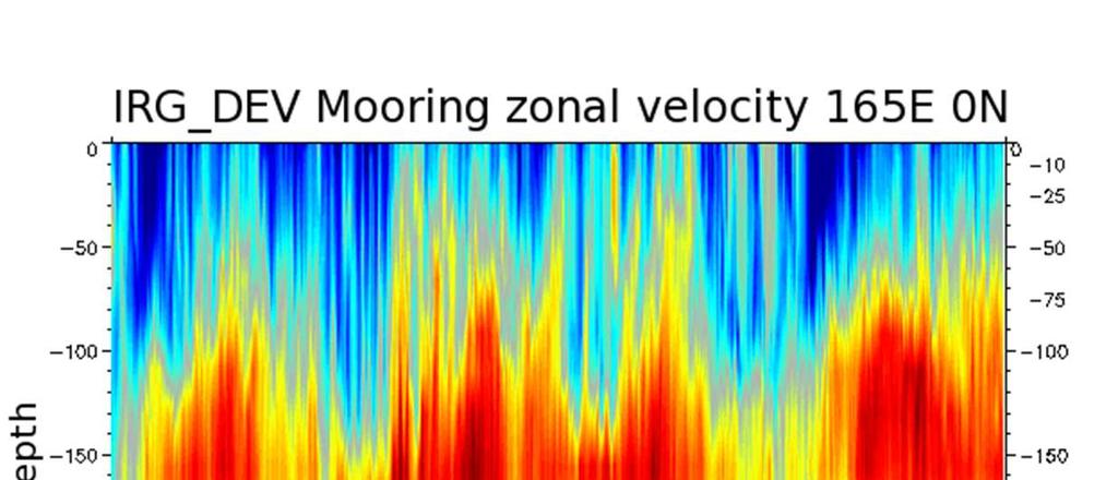
21 J.-M. Lellouche et al.: Global monitoring and forecasting systems at Mercator N over the world ocean. SST longitude time diagrams Fig..Fig. SST.longitude time diagrams at at N over the world ocean. SST from SST from, AVHRR + AMSRE are high-pass fil-at periods AVHRR+AMSRE IRG_VV are, highirg pass VV filtered to keep fluctuations shorter than days. 77 (a) (b) (c) (c) (c) tered to keep fluctuations at periods shorter than days. as illustrated in Fig.. The IRG DEV system assimilates the AVHRR + AMSRE SST product. Consequently, the IRG DEV system is even locally closer to this particular SST product than IRG VV which assimilates RTG (not shown). The HRZ DEV system, like the HRZ VV one, displays TIW that have slightly higher amplitude than the IRG system s TIW in the tropical Atlantic (not shown). 5.. Equatorial Undercurrent We looked more closely at another physical process, the equatorial Pacific current system. Figure shows zonal velocity for equatorial longitude depth sections and latitude depth sections at 65 E. We can see that the IRG VV EUC (Equatorial Undercurrent) does not penetrate west of 65 E and deeper than 00 m. This problem generates an upwelling in the area and changes the water mass properties and transport in the Indonesian Throughflow. The poor representation of the EUC generates errors in the Pacific and Indian Oceans. MDT and its associated error have been adjusted in the IRG DEV experiment by combining the MDT used by the IRG VV experiment and GOCE (Gravity field and steady-state Ocean Circulation Explorer) data. An important consequence of this change is that the EUC is continuous over the whole equatorial Pacific in the IRG DEV experiment, as observed by Johnson et al. (005) and Marin et al. (00). Acoustic Doppler Current Profiler (ADCP) observations, from the TAO/TRITON array of moorings (http: // confirm the improvement of subsurface velocities near 65 E at the Equator. The EUC is well marked in the observations from 007 to 0, and its amplitude of about m s is well represented by IRG DEV, while it is slightly underestimated by IRG VV. 6 Fig.. Zonal velocity (cm s-) equatorial longitude-depth section (a, a, a) and latitude- Fig.. Zonal velocity (cm s ) equatorial longitude depth section (a, a, a) and latitude depth section at 65 E (b, b, b) in the Pacific Ocean. Zonal velocities over depth and time at the 65 E, come from IRG_VV (a, b, c) and IRG_DEV (a, b, c) for the year 00. Mean zonal 0 N, TAO mooring for the period (c, c, c). Zonal sections of ADCP zonal currents come from Johnson et al. (00) (a and b), and from the velocities come from TAO ADCP measurements (c). IRG VV (a, b, c) and IRG DEV (a, b, c) for the year 00. Mean zonal sections of ADCP zonal66currents come from Johnson et al. (00) (a and b) and from the TAO ADCP measurements (c). depth section at 65 E (b, b, b) in the Pacific Ocean. Zonal velocities over depth and time at the 65 E / 0 N TAO mooring for the period (c, c, c). Zonal velocities. Stability in time, trends and biases Regional biases with respect to assimilated and independent data have been identified in the previous sections, and a set of important physical processes have been validated for is now important to verify the long-term behaviour of the It system over the whole period. The linear trend of the temperature at 00 m is estimated with a least squares fit. We call cumulated trend the change due to the trend over the period. The global cumulative trend of temperature at 00 m is shown in Fig. 5. There is a noticeable cooling east of the Philippines and two regions of warming west of Australia in IRG VV (Fig. 5a). These signals are also found in the IRG DEV (Fig. 5b), but the cooling is generally reinforced. The North and South Atlantic are regions of clear cooling in IRG DEV. In several regions, the cumulated trend reaches the IRG DEV bias, as revealed by the 0 temperature innovations near 00 m (Fig. 6b). This cold bias was not found in the 007 innovations (Fig. 6a). This confirms the drift shown in Fig. 0 for the North Pacific. There are other regions where the trend from IRG DEV is not reliable (South Ocean Sci., 9, 57 8, 0

22 78 J.-M. Lellouche et al.: Global monitoring and forecasting systems at Mercator Fig. 5. Cumulative temperature trend ( C) over the period near 00 m for Fig. 5. Cumulative temperature trend ( C) over the peirg_vv and IRG_DEV systems. riod near 00 m for IRG VV and IRG DEV systems. Fig. 6. Mean temperature innovations ( C) near 00 m in 007 and in 0 for IRG_DEV system. Fig. 6. Mean temperature innovations ( C) near 00 m in 007 and in 0 for IRG DEV system. Pacific east of Australia, South Indian between Madagascar and Australia, etc.). The large-scale variability of the surface temperature increments can be assessed with an empirical orthogonal function (EOF) analysis. The first EOF of surface temperature 67 the increment (Fig. 7) gives the major spatial directions of surface temperature correction. The associated time series (principal component) shows the time evolution of this dominant correction pattern. The latter confirms the seasonality of the cold bias observed, in particular in the North Pacific (see Fig. 0). The amplitude of this bias is reduced in the IRG DEV experiment, which indicates that the vertical physics have been improved. The other dominant directions of correction (all variables) are very similar in IRG VV and IRG DEV (not shown). These results suggest that the data assimilation system is not responsible for the general cold trend appearing in IRG DEV and does not accentuate 68 defects of vertical stratification. This confirms the hypothesis of (external) flux correction problems. To conclude, we have identified drifts that can be and must be corrected if these systems are to be used for climate studies. Even though they may be useful for others studies, this stability metric prevents us from releasing the IRG DEV and HRZ DEV systems for the moment. These systems are not ready to replace the existing systems in real time. 5 Conclusions The Mercator Oce an global monitoring and forecasting system (MyOcean V global MFC) has been evaluated for Ocean Sci., 9, 57 8, 0 Fig. 7. st EOF of surface temperature increment made every 7 days ( C) over the Fig. 7.IRG_VV st EOF ofirg_dev surfacetemperature made every period for and systems. The timeincrement series at the bottom of each 7panel days ( C)toover the period for IRG VV and correspond the mode amplitude. IRG DEV systems. The time series at the bottom of each panel corresponds to the mode amplitude. the period by means of a thorough procedure involving statistics of model departures from observations and assessment of physical processes. The accuracy of the V system (including the global / IRG VV and its / North Atlantic and Mediterranean zoom HRZ VV) is clearly better than the climatology. Performances are stable over time and should be reliable in the long term. All monitoring systems are close to SLA observations with a forecast (range to 7 days) RMS difference of 7 cm. This is smaller than the intrinsic variability of the SLA observations. The dominant source of error in sea level comes from the uncertainty in the MDT. The global IRG gives an accurate description of water masses almost everywhere between the ocean bottom and 500 m. Within such layers, de69 partures from in situ observations decrease with the depth and do not exceed 0. C for temperature and 0.0 psu for salinity. Between 0 and 500 m, departures from in situ observations rarely exceed C and 0. psu. Exceptions concern some high variability regions such as the Gulf Stream or the eastern tropical Pacific. Most departures from SST products do not exceed the intrinsic error of these products O(0.6 C). During the summer season, the upper ocean is not vertically stratified enough. Excess mixing results in cold biases near the surface and warm biases in subsurface. This bias is particularly marked in IRG DEV and leads to a large-scale bias of more than C for the boreal summer in the North Pacific Gyre where the mixed layer is already thin. The bias can be attributed to the atmospheric forcing and/or the biooptic properties of the seawater. The system is not efficient enough in correcting the SST because heat fluxes are not included in the estimated state. A detailed study reveals that most of the SST correction provided by the analysis is swept away by the bulk forcing function. A comparison with independent velocity measurements (surface drifters) shows that the surface currents are underestimated in the mid latitudes and overestimated at the Equator with respect to windage and slippage-corrected drifter velocities. This correction developed by Mercator Oce an has been applied to cope with the drogue loss of the surface drifter. The underestimation ranges from 0 % in strong currents up