Eddy-resolving global ocean prediction

Transcription

1 Eddy-resolving global ocean prediction Harley E. Hurlburt 1, Eric P. Chassignet 2, James A. Cummings 1, A. Birol Kara 1, E. Joseph Metzger 1, Jay F. Shriver 1, Ole Martin Smedstad 3, Alan J. Wallcraft 1, and Charlie N. Barron 1 1 Naval Research Laboratory Oceanography Division Stennis Space Center, MS Center for Ocean-Atmospheric Prediction Studies Florida State University 200 R. M. Johnson Bldg. Tallahassee, FL Planning Systems, Inc. Stennis Space Center, MS Chapter for an AGU Monograph entitled Eddy-Resolving Ocean Modeling 2 Nov

2 ABSTRACT Global prediction of the ocean weather (e.g. surface mixed layer, meandering currents and fronts, eddies, and coastally trapped waves) has been feasible only since the turn of the century when sufficient computing power and real-time data became available. Satellite altimetry is the key observing system for mapping ocean eddies and current meanders, but sea surface temperature, temperature and salinity profiles, and atmospheric forcing are also essential. The multinational Global Ocean Data Assimilation Experiment (GODAE) has fostered the development of eddy-permitting and eddy-resolving basin-scale to global prediction systems in several countries. Here, the focus is eddy-resolving global ocean prediction, the value of ocean model skill in dynamical interpolation of data and in forecasting, plus the increased skill gained from using eddy-resolving versus eddy-permitting models. In ocean prediction one must consider the classes of ocean response to atmospheric forcing for different phenomena and regions. In ocean nowcasting, this is important in considering the relative impact of the atmospheric forcing and different ocean data types. In forecasting, these classes impact whether or not the timescale for oceanic predictive skill is limited by the timescale for atmospheric predictive skill, or whether a coupled ocean-atmosphere model would be advantageous. Results from the existing eddy-resolving global ocean prediction systems demonstrate forecast skill up to one month, globally, and over most subregions. Outside surface boundary layers and shallow water regions, the forecast skill typically is only modestly impacted by reverting toward climatological forcing after the end of the atmospheric forecast versus using analysis-quality forcing for the duration. 2

3 1. INTRODUCTION Adequate real-time data input, computing power, numerical ocean models, data assimilation capabilities, atmospheric forcing, and bottom topography are key elements required for successful eddy-resolving global prediction of the ocean weather, such as the surface mixed layer, equatorial and coastally trapped waves, upwelling of cold water, meandering of currents and fronts, eddies, Rossby waves, and the associated temperature, salinity, currents, and sea surface height (SSH). Only since the turn of the century have all the key elements finally reached a status that makes global ocean weather prediction feasible. The focus of this chapter is on the roles that eddy-resolving ocean models perform in accurate nowcasting (estimating the present state) and forecasting of the ocean weather on timescales up to a month. However, much of the content is also relevant to climate prediction. In the remainder of the introduction the relevance of this chapter to climate is briefly discussed in section 1.1. Section 1.2 outlines the history of the first 10 years of basin-scale to global ocean weather prediction, the product of a multinational effort largely fostered by the Global Ocean Data Assimilation Experiment (GODAE). In section 1.3 ocean prediction is discussed in relation to four classes of ocean response to atmospheric forcing, how they impact ocean prediction, and how they affect the involvement of ocean models. Section 2 presents results illustrating the roles that ocean models play in nowcasting and forecasting with emphases on results from eddy-resolving global ocean models and prediction systems and the relation to classes of responses to atmospheric forcing. These include dynamical interpolation of assimilated data, the 3

4 value of atmospheric forcing as a data type, sensitivity to ocean model resolution (e.g. eddy-resolving versus eddy-permitting and impact on the space scales that can be mapped using nadir beam satellite altimetry), use of mean SSH from an eddy-resolving global ocean model in creating a mean SSH field for addition to the anomalies from satellite altimetry, and the use of simulated data from eddy-resolving ocean models in testing, evaluating, and improving data assimilation skill. The latter is also an example of observing system simulation and assessment. 1.1 Relevance to climate To date, multidecadal climate prediction models and seasonal to interannual climate forecasts (focused primarily on El Niño/La Niña conditions) have used coarse resolution ocean models that are unable to depict realistic ocean fronts. As climate predictions become increasingly region specific, eddy-resolving ocean models will be required for success in many regions, e.g. for accurate positioning, strength, and eastward penetration of major ocean currents and fronts. As specific examples, eddy-resolving ocean models are required for realistic prediction of the Kuroshio/Oyashio current system in the western North Pacific and the Gulf Stream current system in the western North Atlantic. In the Pacific such models must simulate a strongly inertial Kuroshio with sufficient eastward penetration and advection of heat as well as cold southward currents along the east coast of Japan rather than the warm northward flow found in coarse resolution models. Eddy-resolving models are also needed to obtain the sharp ocean fronts that span the entire North Pacific [Hurlburt et al., 1996; Hurlburt and Metzger, 1998]. In the North Atlantic, eddy-resolving models are required to accurately simulate 4

5 the Gulf Stream pathway between Cape Hatteras and the Grand Banks and to obtain the associated large nonlinear recirculation gyres in this region [Hurlburt and Hogan, 2000; Bryan et al., 2007]. These large nonlinear gyres change the large-scale shape of the subtropical gyre into a C-shape. East of the Grand Banks the Gulf Stream turns northward as the North Atlantic Current, and an eddy-resolving model is essential for the model to advect sufficient heat northward and then eastward across the Atlantic at around 50 N [Smith et al., 2000]. These are examples of regions where errors caused by coarse resolution in ocean global circulation models (OGCMs) would lead to large errors in climate anomaly or climate change predictions for North America, Europe, the Arctic, and Japan. 1.2 Ocean weather prediction, a brief history of the first 10 years GODAE [Smith, 2000, 2006] has been a major driving force behind a multinational effort working toward the development of eddy-resolving global ocean prediction capabilities in different countries. Australia, Britain, France, Japan, and the United States are all sponsoring efforts that are presently in various stages toward reaching this goal (see the book by Chassignet and Verron [2006] for an overview). The Forecasting Ocean Assimilation Model (FOAM) system, developed by the Met Office UK, became the first operational global ocean prediction system in 1997, but at 1 resolution it was non-eddy resolving [Bell et al., 2000]. Ten years later the availability of sufficient computer resources is still a significant limiting factor in ocean weather prediction. Hence a variety of approaches and trade-offs have been used to work toward the eddy-resolving global goal. All of the remaining global and basin-scale 5

6 prediction systems considered here are either eddy-permitting or eddy-resolving, and all include some form of altimeter data assimilation. SSH from satellite altimetry is the key available data type for mapping the ocean weather in deep water [Hurlburt, 1984]. Basin-scale prediction systems have been a common step toward the global goal, either nested in a coarser resolution global system (the Met Office UK) or standalone (the remainder). Such systems started at 1/3 resolution in January 2001 (British FOAM Atlantic/Arctic and Indian Ocean, French MERCATOR North and tropical Atlantic). These were soon followed by higher resolution basin-scale systems (1/9 British FOAM North Atlantic/Mediterranean Sea since 2002, operational in 2004 [Bell et al., 2006]; the French MERCATOR 1/15 North Atlantic plus 1/16 Mediterranean Sea operational in January 2003 [Bahurel, 2006], and a 1/12 Atlantic system run in demonstration mode by the HYbrid Coordinate Ocean Model (HYCOM) Consortium in the U.S. since July 2002 [Chassignet et al., 2007]). Some of the basin-scale systems have used variable resolution focused on a region of interest. The Norwegian DIADEM (later TOPAZ) Atlantic and Arctic system [Bertino and Evensen, 2002] has been running since 2001 using a curvilinear grid with km resolution (increased to km in July 2007) with the highest resolution focused on the northeast Atlantic and Nordic Seas. Since 2001 the Japan Meteorological Agency (JMA) has been running a daily operational North Pacific assimilation-prediction system COMPASS-K (12 N to 55 N) with variable latitude and longitude resolution as high as 1/4 in the western North Pacific around Japan [Kamachi et al., 2004a, 2004b], and in 2007 the Japanese Meteorological Research Institute began running a real-time ocean data assimilation and prediction system MOVE/MRI.COM-NP covering the Pacific 6

7 Ocean (15 S 65 N) with variable latitude and longitude resolution as high as 1/10 near Japan [Usui et al., 2006a, 2006b, Tsujino et al., 2006, Usui et al., 2007]. The U. S. National Oceanic and Atmospheric Administration/National Centers for Environmental Prediction (NOAA/NCEP) has been running a real-time HYCOM equatorial and North Atlantic prediction system with assimilation of satellite altimeter data added on 28 June The horizontal resolution is about 4 to 18 km with the highest resolution focused in the Gulf of Mexico and along the east coast of North America. Crosnier and Le Provost [2007] performed an inter-comparison study of five basin-scale prediction systems run in five different countries covering the North Atlantic and/or the Mediterranean Sea [the 1/9 British FOAM North Atlantic/Mediterranean Sea system, the French MERCATOR 1/15 North Atlantic/1/16 Mediterranean Sea system, the U.S. 1/12 Atlantic HYCOM system, the HYCOM-based Norwegian TOPAZ Atlantic/Arctic system, and the Italian MFS 1/8 (later 1/16 ) Mediterranean Sea system]. Of these, three use fixed-depth z-level models and two use HYCOM. The latter has a generalized vertical coordinate that allows Lagrangian isopycnal layers, pressure levels (~z-levels), terrain-following and other vertical coordinates [Bleck, 2002; Chassignet et al., 2003; Halliwell, 2004; Chassignet et al., 2007]. Another approach is that of the Shallow-Water Analysis and Forecast System (SWAFS) North World, developed at the Naval Oceanographic Office (NAVOCEANO). SWAFS used the Princeton Ocean Model (POM) with terrain-following coordinates [Blumberg and Mellor, 1987]. This system covered the world ocean over the latitude range 20 S to 80 N with ~1/5 (~23 km) mid-latitude resolution. Effectively, it was a convenient way to run multiple basin-scale models within one model domain, since the 7

8 basins are disconnected at the southern boundary and, although the Indonesian Archipelago is included, the Indonesian throughflow is largely blocked because of the southern boundary. The SWAFS North World system was run at NAVOCEANO from 1998 to 2006, but never became operational. A SWAFS system of similar design for the Mediterranean Sea [Horton et al., 1997] did become an operational prediction system. Global ocean prediction systems that make various compromises to cope with limitations in available computing power have also been developed. A 1/4 global French MERCATOR system with 46 levels in the vertical has been running operationally since October 2005 [Bahurel, 2006]. The Australian BLUElink global ocean prediction system has 1/10 resolution on a 90 latitude and longitude sector surrounding Australia, variable resolution as coarse as 2 elsewhere and 47 levels in the vertical [Schiller and Smith, 2006]. The BLUElink system became operational in July All of the preceding systems have coordinate surfaces in the vertical direction. The U. S. Navy has used a still different approach in its present operational global ocean prediction systems, a linked two-model approach [Rhodes et al., 2002]. One model has high horizontal resolution but low vertical resolution, while the other has high vertical resolution but lower horizontal resolution. The earliest version of this system used only the model with low vertical resolution, the Naval Research Laboratory (NRL) Layered Ocean Model (NLOM). It had six Lagrangian layers in the vertical and 1/4 resolution globally, excluding the Arctic and most shallow water [Metzger et al., 1998a,b]. It was the first global ocean weather prediction model to assimilate real-time satellite altimeter data (from TOPEX/Poseidon and ERS-2) and ran daily in real time from 1997 to 2000 at the Fleet Numerical Meteorology and Oceanography Center 8

9 (FNMOC) but never became operational. In 2000 NAVOCEANO became the U. S. Navy center for numerical prediction of the ocean weather. A mixed layer (seventh layer) [Wallcraft et al., 2003] was added to the NLOM-based component of a system for NAVOCEANO, which began running daily in real time with 1/16 resolution on 18 October It ran operationally from 27 September 2001 to 11 March 2006, thereby becoming the first operational eddy-resolving global ocean prediction system [Smedstad et al., 2003]. A 1/32 version of this system began running in near real time on 1 November 2003, real time since 1 March 2005 and replaced the 1/16 system as the operational system on 6 March 2006 [Shriver et al., 2007]. The second component of the NAVOCEANO system uses the Navy Coastal Ocean Model (NCOM) and has 1/8 (~15 km) mid-latitude resolution, 1/6 (~19 km) tropical resolution, 40 levels in the vertical and is fully global [Barron et al., 2006; Kara et al., 2006]. It has been running daily in real time since October 2001 and became operational on 19 February The NLOM component is used to assimilate SSH data along altimeter tracks with a model forecast as the first guess for each analysis cycle and it is used to make 30-day ocean weather forecasts. It also assimilates model-independent analyses of sea surface temperature (SST). The NCOM component assimilates steric SSH anomalies from NLOM in the form of synthetic temperature and salinity (T & S) profiles [Rhodes et al., 2002]. These profiles are obtained from surface dynamic height and SST anomalies by means of regression equations for subsurface temperature and T & S relations for salinity, both using statistics derived from the historical hydrographic data base [Carnes et al., 1990; Fox et al., 2002]. This two-model global system requires less 9

10 computer power than a single global model with both high horizontal and high vertical resolution, which is the goal of most GODAE participants. The U. S. Navy began running the first eddy-resolving global system with high vertical resolution in near real time on 22 December 2006 and it has been running in real time since 16 February This system uses a fully global configuration of HYCOM with 1/12 equatorial (~7 km mid-latitude) resolution and 32 layers in the vertical. Each day it performs a five-day hindcast (assimilation of data prior to the real-time data window) at one-day increments to pick up delayed data and it makes a five-day forecast. In addition, tests of 30-day forecasts have been performed. Although limitations on ocean model domain size and resolution have been essential in dealing with limitations in available computer power, computing requirements have also been economized though the choice of data assimilation techniques and assimilated data sets. Also, while most of the preceding systems run daily in real time, computing requirements for other systems have been reduced by running in near real time and updating once a week, rather than daily. 1.3 Ocean prediction in relation to classes of ocean response to atmospheric forcing Table 1 is a summary of some useful classes of ocean response to atmospheric forcing that cover many phenomena of potential interest in ocean prediction. In developing an ocean prediction system, it is essential to consider these classes and their implications for (a) data requirements, (b) the time scales of oceanic predictive skill, and (c) prediction system design. 10

11 In the case of Class 1 phenomena, characterized by strong and rapid development (less than a week), ocean model simulation skill plays a critical role in converting atmospheric forcing into oceanic information. The timescale for oceanic forecast skill is largely determined by the timescale for atmospheric predictive skill, and the influence of anomalies in the initial state rapidly decreases. The timescale for oceanic predictive skill may exceed that for the atmosphere to some extent because of lagged responses, the influence of geometric or topographic constraints, or the initiation of Class 4 free waves or ocean eddies. Such phenomena are commonly found in shallow water where rapid barotropic responses are particularly important, within the surface mixed layer or Ekman layer, in equatorial and coastal wave guides, and in the vicinity of hurricanes or other strong wind events (e.g. wind-driven eddies in the Gulf of Tehuantepec). In section 2.7 some examples are given in which Class 1 anomalies lead to Class 4 anomalies or where Class 1 and Class 4 phenomena interact to generate new Class 4 features. Nowcasting and forecasting of Class 1 phenomena place high demands on the accuracy of the ocean model and the atmospheric forcing. In shallow water and near coastal boundaries, there are additional demands for accurate topography and coastlines, tides, and fine resolution atmospheric forcing. Near coastlines it is important that atmospheric values over land are not used as forcing at ocean model grid points, a common problem in fine resolution ocean models forced by a coarser resolution atmospheric product [Kara et al., 2007a]. When ocean data are assimilated, the model time and the observation time must closely match because of the rapid evolution; but even so, the ocean data may rapidly lose impact after assimilation. 11

12 Class 2 phenomena (slower and indirectly forced) tend to be a largely nondeterministic response to atmospheric forcing due to flow instabilities, e.g. the generation of mesoscale eddies and the meandering of ocean currents and fronts. Thus ocean data assimilation is essential to nowcast and forecast these features, and the nowcast and forecast results are relatively insensitive to the atmospheric forcing, allowing forecasts up to a month or more. SSH anomalies measured by satellite altimetry are the key data that all of the GODAE participants use to map these mesoscale features, as well as many other features, including El Niño and La Niña events. SSH is a particularly useful data type observable from space because (a) it is geostrophically related to surface currents, (b) it is an integral measure of subsurface variations in T & S (e.g., the depth of the thermocline) plus a bottom pressure anomaly, and (c) the oceanic vertical structure is generally low mode. Thus it has been possible to develop a number of techniques to project the SSH anomalies downward, in some cases including the bottom pressure anomaly (the nonsteric contribution to SSH). These techniques range from model dynamics [Hurlburt, 1986], to model statistics [Hurlburt et al., 1990], to a potential vorticity constraint [Cooper and Haines, 1996], to data assimilation covariances, to synthetic T & S profiles estimated from a combination of SSH and SST related by regression to the historical hydrographic data base [DeMey and Robinson, 1987; Carnes et al., 1990; Fox et al., 2002]. The regions of the global ocean dominated by Class 2 variability can be estimated by calculating the fraction of variability of different ocean variables (e.g. SSH, SST, eddy kinetic energy (EKE), and bottom pressure) that is a nondeterministic response to atmospheric forcing in eddy-resolving model simulations [Metzger et al., 1994; Hurlburt 12

13 and Metzger, 1998; Metzger and Hurlburt, 2001; Melsom et al., 2003; Hogan and Hurlburt, 2005]. Although areas that are highly nondeterministic are not necessarily regions of high SSH variability or EKE, it is relevant to evaluate the model against its ability to simulate regions of high variability. In addition, ocean forecast skill beyond the range of atmospheric predictive skill can be verified. The sensitivity of ocean forecast skill to atmospheric forcing can be tested versus persistence (a forecast of no change) and by comparing the skill of forecasts performed using analysis quality forcing versus forecasts reverting toward climatological forcing beyond the end of the forecast forcing [Smedstad et al., 2003; Shriver et al., 2007, section 2 of this chapter] (relevant to all four classes of oceanic response). Class 3 phenomena (slow, direct integrated responses to atmospheric forcing on timescales of weeks to years) are perhaps more relevant to seasonal to interannual prediction (e.g. El Niño and La Niña events) using coupled ocean-atmosphere models. However, Class 3 phenomena are also relevant to uncoupled models and shorter range predictions. They are relevant to both types of prediction when considering the role of uncoupled models in determining the mean SSH added to SSH anomalies from satellite altimetry, a topic discussed in section 2.6. The required mean SSH contains a wide range of space scales, some of which are adequately resolved only in simulations by a high resolution model. This places a heavy burden on the accuracy of the ocean model and the atmospheric forcing. In addition, Class 3 phenomena are important in nowcasting and forecasting some ocean features that are inadequately observed, e.g. for an eddy-resolving model, the seasonal cycle of mixed layer depth (MLD) and anomalies in MLD lasting longer than 13

14 the Class 1 timescale of skillful atmospheric weather prediction, examples where a Class 3 response to atmospheric forcing will have a much larger impact than assimilation of ocean data. Presently, ~3000 Argo floats [Roemmich et al., 2004] profile T & S down to typical depths of 2000 m with high vertical resolution. These floats constitute an accurate observing system for measuring subsurface T & S, including MLD, but one that, while suitable for climate, is too sparse horizontally and temporally to constrain an eddyresolving ocean model, and too sparse to constrain MLDs in any model on Class 1 timescales. As discussed in Hurlburt et al. [2001], 3000 Argo floats, arrayed like an altimeter, could provide horizontal coverage at a single level (e.g. MLD or surface dynamic height) which is only ~4% of that from one Jason-1 altimeter over its 10-day orbital repeat cycle. This comparison is based on placing Argo floats along over-water altimeter tracks at 50 km intervals and profiling at 10-day intervals. Class 4 phenomena consist of free propagation of ocean features that exist in the initial state of the forecast, i.e. features generated earlier as Class 1, 2, or 3 phenomena. In addition to examples mentioned in the discussion of Class 1 phenomena, Kelvin waves generated by El Niños have propagated cyclonically around the North Pacific as far as Alaska and the Kamchatka Peninsula of Russia in both observations and models [Metzger et al., 1998a; Melsom et al., 2003]. Jacobs et al. [1994] even demonstrated a decadelong forecast of a trans-pacific non-dispersive internal Rossby wave, generated from the El Niño, which eventually displaced the Kuroshio Extension east of Japan. The forecast used climatological atmospheric forcing (a corresponding simulation with interannual forcing was also run), and the forecast was verified using satellite altimetry and other data. In addition to wind-generated eddies (like Tehuantepec eddies), stable 14

15 isolated eddies that are products of flow instability, but which escape any region of strong flow instability, may belong to Class 4. Such eddies can last for over a year [Lai and Richardson, 1977], although they are unlikely to be predictable for nearly that long. Nowcasting is an essential step in ocean monitoring and prediction of all the classes of oceanic response in Table 1. To perform a nowcast, a numerical model forecast is used as the first guess for assimilation of new data. This use of the forecast allows the model (1) to help fill in the temporal and spatial gaps between observations (including temporal gaps between the repeat cycles of satellite altimetry) and make effective use of delayed data by exploiting its predictive skill, (2) to help convert the better-observed surface fields into subsurface structure [Hurlburt, 1986], (3) to convert the better-observed atmospheric forcing functions into useful oceanic responses, and (4) to apply bottom topography, coastline geometry, and the ocean surface as physical and dynamical constraints with associated boundary layers. Partially in conjunction with a barotropic model [Carrere and Lyard, 2003], the model component of the ocean prediction system can also help separate the steric and non-steric contributions to SSH, a significant capability in the assimilation of satellite altimeter data [Rhodes et al., 2002]. Examples of the preceding model contributions to nowcast and forecast skill (without a reference) are illustrated in section 2. There is an important difference between data assimilation in oceanography and meteorology. In oceanography there is a greater burden on the models to extract information from the data, including use of the models to extract oceanic responses to atmospheric forcing as well as converting surface information into subsurface information, which is sparsely observed. In addition, an eddy-resolving global ocean 15

16 model should play a major role in determining the mean SSH used in assimilation of satellite altimeter data (discussed in section 2) and it may be used as a source of covariances and other statistics for data assimilation. Therefore models play a crucial role in making effective use of the data sources and in reducing data requirements in ocean nowcasting in addition to their essential role in ocean forecasting. Other applications of eddy-resolving ocean models in ocean prediction include understanding model and ocean dynamics, assessing and improving the realism of the ocean model, studying ocean model resolution requirements, performing oceanic predictability studies, investigating the classes of response to atmospheric forcing in different dynamical regimes, and providing realistic simulated data (a) for data assimilation studies, (b) for studies of data base requirements and observing system simulation experiments (OSSEs), and (c) for spinning up models to the initial time when data assimilation begins. Eddy-resolving models can also be used to investigate model sensitivity to the choice of atmospheric forcing product, although a linear barotropic numerical model with realistic deep water boundaries (essentially Sverdrup [1947] interior flow with Munk [1950] viscous western boundary layers consistent with the Godfrey [1989] island rule) can be very useful for this purpose with much lower computational requirements [Townsend et al., 2000; Hogan and Hurlburt, 2005]. A number of the issues raised in this subsection are illustrated and discussed in section 2. 16

17 2. EDDY-RESOLVING GLOBAL OCEAN PREDICTION SYSTEMS Here we focus on the only two existing eddy-resolving global ocean prediction systems to date, the 1/16 (later 1/32 ) NLOM-based system with low vertical resolution and the more recent 1/12 global HYCOM-based system, which has both high horizontal and high vertical resolution. HYCOM is fully global, unlike NLOM, which excludes the Arctic and most shallow water. The results presented are used in the illustration and discussion of some key issues in ocean weather prediction. 2.1 The HYCOM and NLOM prediction systems Both HYCOM and NLOM have a free surface and use a Lagrangian vertical coordinate to model the ocean interior. However, simplifications are made in NLOM that make it much more computationally efficient, but which limit its range of application and versatility, while the generalized vertical coordinate and the allowance of zero thickness layers make HYCOM extremely versatile and suitable for a wide range of ocean modeling applications. General details of NLOM design and progressive development are discussed in Hurlburt and Thompson [1980], Wallcraft [1991], Wallcraft and Moore [1997], Moore and Wallcraft [1998], and Wallcraft et al. [2003]. The last of these discusses the development of NLOM as a thermodynamic model with a Kraus and Turner [1967] type bulk mixed layer and SST. This version of NLOM was used in the 1/16 and 1/32 global prediction systems listed in section 1.2. More specifically, the resolution for each variable is 1/16 (1/32 ) in latitude and 45/512 (45/1024 ) in longitude or ~7 km (3 4 17

18 km) at mid-latitudes in the 1/16 (1/32 ) system. The NLOM domain is nearly global, extending from 72 S to 65 N, with the model boundary generally following the 200-m isobath with a few exceptions, like the shallow straits connecting the Sea of Japan (East Sea) to the Pacific Ocean. NLOM uses vertically compressed but otherwise realistic bottom topography confined to the lowest layer [Hurlburt et al., 2007]. Sill depths of straits that are shallower than the bottom layer are maintained by constraining the flow to small values below the sill depth [Metzger and Hurlburt, 1996]. The reduced amplitude of the topography generally does not have a significant impact on the abyssal current steering of upper ocean current pathways (an essential capability of eddy-resolving ocean models which simulate eddy-driven abyssal currents), because even low amplitude topographic features can constrain the pathways of abyssal flow [Hurlburt and Metzger, 1998; Hurlburt et al., 2007]. Deep water formation outside the model domain is included via prescribed observationally-based transports through four straits in the northern boundary of the North Atlantic, northward in the upper layers and southward in the bottom layer [Shriver and Hurlburt, 1997]. The history of NLOM use in ocean prediction systems was given in section 1.2. Each day the NLOM prediction system performs a hindcast at daily increments to pick up delayed altimeter data (a five-day hindcast for the 1/32 system, a three-day hindcast for the former 1/16 system) and it makes a four-day forecast (plus a 30-day forecast once a week) [Smedstad et al., 2003; Shriver et al., 2007]. NLOM assimilates along-track satellite altimeter data using the model as a first guess for the SSH analysis, and it assimilates SST in the form of daily operational model-independent SST analyses from NAVOCEANO [Barron and Kara, 2006]. The SSH assimilation process consists of an 18

19 optimum interpolation (OI) deviation analysis from the model first guess and an empirical orthoganal function (EOF) regression technique based on model statistics to project the SSH updates downward, including to the abyssal layer [Hurlburt et al., 1990]. These updates are geostrophically balanced outside the equatorial region and inserted incrementally to further reduce inertia-gravity wave generation. Anisotropic, spatiallyvarying mesoscale covariance functions determined from TOPEX/Poseidon and ERS-2 altimeter data [Jacobs et al., 2001] are used in the OI analysis. The SST assimilation consists of relaxing the analysis into the model. HYCOM has been developed as a collaborative multi-institutional effort starting from the Miami Isopycnic Coordinate Ocean Model (MICOM) using the theoretical foundation set forth in Bleck and Boudra [1981], Bleck and Benjamin [1993], and Bleck [2002]. HYCOM uses a generalized vertical coordinate that is normally isopycnal in the open stratified ocean, with a dynamically smooth transition to pressure coordinates (~zlevels) in the unstratified mixed layer and to σ (terrain-following) coordinates in shallow water, but it is not limited to these types. The transition between coordinate types is made dynamically in space and time using the layered continuity equation and a hybrid coordinate generator. This generalized coordinate approach retains particular advantages associated with the different vertical coordinate types: (1) the retention of water mass characteristics for centuries (a characteristic of the isopycnal coordinate interior), (2) high vertical resolution in the surface mixed layer and unstratified or weakly stratified regions of the ocean (a characteristic of z-level coordinates), and (3) high vertical resolution in coastal regions (a characteristic of terrain-following coordinates) [Chassignet et al., 2003]. The generalized coordinate also facilitates accurate transition between deep and 19

20 shallow water and allows the use of a sophisticated embedded mixed-layer model in an ocean model with an isopycnal interior, e.g. a K-profile parameterization (KPP) [Large et al., 1997] in the ocean prediction system. For the 1/12 global HYCOM, the model resolution south of 47 N is exactly 0.08 by 0.08 cos(latitude) for each variable (~7 km at mid latitudes) and is described by the approximate equatorial resolution. A bipolar grid is used north of 47 N, resulting in a tripole global grid [Murray, 1996], which gives ~3.5 km resolution in the Arctic. The model includes 32 hybrid coordinate surfaces in the vertical direction and is run with thermobaricity [Sun et al., 1999; Chassignet et al., 2003; Hallberg, 2005] using a reference depth of 2000 db for potential density, a model configuration known as σ 2 *. The 1/12 global HYCOM prediction system has been running daily in near real time since 22 December 2006 and in real time since 16 February Even more than for the NLOM system, because HYCOM includes shallow water, doubling the resolution is desirable when the computing power becomes available. The impact of model resolution is a recurring theme in the rest of section 2. The data are assimilated into HYCOM using the Navy Coupled Ocean Data Assimilation (NCODA) system of Cummings (2005) with a modification described in section 2.8. Within NCODA, a HYCOM forecast is used as the first guess for a multi-variate optimum interpolation (MVOI) [Daley, 1991] analysis of SSH track data from satellite altimetry, SST, and T & S profiles. The analysis is then inserted incrementally into HYCOM. In the analysis, Cooper and Haines [1996] is used for downward projection of SSH below the mixed layer, although downward projection of SSH and SST using synthetic T & S profiles 20

21 [Fox et al., 2002] is also an option in NCODA. The updates to the mass field are geostrophically balanced outside an equatorial band /16 eddy-resolving versus 1/4 eddy-permitting models in nowcasting and forecasting the Kuroshio Extension Figure 1 illustrates the relative dynamical interpolation (nowcast) and forecast skill of 1/4 eddy-permitting versus 1/16 eddy-resolving six-layer versions of NLOM in the Kuroshio Extension region east of Japan, as verified by NAVOCEANO operational 1/8 Modular Ocean Data Assimilation System (MODAS) model-independent SST analyses [Barron and Kara, 2006] with the color bar designed to highlight the Kuroshio pathway. The 1/16 Pacific prediction system discussed here is the forerunner of the 1/16 global NLOM prediction system which later became operational at NAVOCEANO, except that it lacked a mixed layer and SST [Hurlburt et al., 2000; Metzger et al., 2000]. The 1/4 global system is one of two versions run in real time at FNMOC (section 1.2). Results for 1 January and 15 January 1999 are shown for each product. Two-week forecasts from 1 January for each model can be compared with the three analyses for 15 January. The model nowcasts were updated daily with assimilation of altimeter track data from TOPEX/Poseidon and ERS-2 using a three-day window (red tracks overlaid on two of the plots) and the methodology outlined in section 2.1 for NLOM. Because the geoid of the Earth is not adequately known, only the altimetric deviations from their own mean are useful in the assimilation. In the model assimilations a slightly modified mean from the corresponding model was added to these deviations. Generally, the two means agree closely, but the 1/16 model gives a sharper 21

22 depiction of mean currents and a sharper depiction of the Kuroshio in the nowcast and forecast results. Several features are clearly evident in the SST and the model results. Here we focus on the sharp meander between 155 E and 160 E on 1 January 1999, which evolved into a distinctive eddy detachment in progress on 15 January. This sequence is captured with striking agreement between the SST analyses, the 1/16 model nowcasts, and the 1/16 model forecast. The 1/4 model represents the sharp meander on 1 January quite well but the 1/4 nowcast for the detaching eddy on 15 January is poor and the 15 January 1/4 model forecast for this feature is a very unrealistic meander contraction. These results are a demonstration of ocean model eddy-resolving nowcast and forecast skill using satellite altimeter data. In particular, the results demonstrate (1) that satellite altimetry can be an effective observing system for mapping and forecasting mesoscale ocean features, (2) that an ocean model with high enough horizontal resolution can be a skillful dynamical interpolator of satellite altimeter data in depicting mesoscale oceanic variability, and (3) that an eddy-resolving ocean model can provide skillful forecasts of mesoscale variability when a model with assimilation of altimeter data is used to define the initial state, in this example for the duration of the 31-day forecast [Hurlburt et al., 2000]. It is worth noting that this was the very first forecast performed with the 1/16 Pacific model used here, not the best of many. In contrast, the 1/4 global model had insufficient horizontal resolution, lower skill as a dynamical interpolator, and poor forecast skill, with a strong tendency to damp the variability. The broadening of the Kuroshio in the 1/4 model means the current speeds are lower, and dynamically the 22

23 current is not as inertial, a clear indication that one should anticipate a substantial impact on model forecast skill and skill as a dynamical interpolator. The 1/16 Pacific model used for assimilation of real altimeter data in Figure 1 was also used in testing assimilation of simulated altimeter track data derived from the model along ERS-2, GFO, and both sets of TOPEX/Poseidon repeat tracks. Simulated altimeter data from model year 1994 were assimilated into the model starting from an initial state in model year 1997, a time when the model Kuroshio pathway was quite different. Compared to no assimilation or a model mean, large error reduction was obtained in all six layers of the model, including the abyssal layer, after about a month of simulated altimeter data assimilation. This was true even when simulated data from only one of the altimeters (any one of them) were assimilated. The error was significantly reduced by adding a second altimeter with the tandem tracks of Jason-1 and TOPEX/Poseidon clearly performing the best. Only modest error reduction was obtained by adding a third altimeter [Hurlburt et al., 2000; Smedstad et al., 2003]. 2.3 Impact of resolution that is eddy-resolving versus eddy-permitting on model dynamics and simulation skill Because of its relative computational efficiency and simplicity, NLOM has been used to perform a number of studies investigating the impact of increasing the horizontal resolution as well as the impact of other aspects of model design on (a) model dynamics, (b) simulation skill, (c) convergence of the mean circulation and variability in relation to mesoscale features, and (d) agreement with observations in different regions of the world ocean. Most of these studies were performed without ocean data assimilation. 23

24 For the Kuroshio near Japan (west of ~155 E), Hurlburt et al., [1996, 1997] found that 1/8 (~15 km) mid-latitude resolution was sufficient to simulate a realistic Kuroshio pathway, including the mean meanders observed east of Japan. This simulation included vertically compressed but otherwise realistic bottom topography. Corresponding models with 1/4 resolution or with 1/8 resolution and a flat bottom gave unrealistic simulations of the Kuroshio in this region. The mean Kuroshio pathway was realistic in the 1/8 simulation with topography because it simulated upper ocean topographic coupling via mixed baroclinic-barotropic instabilities [Hurlburt et al., 1996]. This coupling occurs when baroclinic instability transfers energy to the abyssal layer where it is constrained to follow the geostrophic contours of the bottom topography. The eddy-driven mean abyssal currents, in turn, advect upper ocean current pathways, especially where these currents intersect at large angles. In the advection process there is often a natural tendency toward barotropy, because the current pathway advection is reduced when this occurs. In the example considered here, a modest seamount complex just east of Japan played a critical role in steering a mean meander in the Kuroshio pathway immediately east of Japan, thus affecting the separation of the Kuroshio from the east coast of Japan. Most of the references in this subsection discuss upper ocean topographic coupling via flow instabilities and a theory for steering of upper ocean current pathways by abyssal currents, which is discussed most comprehensively in Hurlburt et al. [2007]. East of 155 E, Hurlburt et al. [1996] and Hurlburt and Metzger [1998] found that 1/8 resolution is insufficient and 1/16 is sufficient to simulate the eastward penetration of the Kuroshio as an inertial jet, the bifurcation of the Kuroshio at the Shatsky Rise, and 24

25 sharp fronts that span the northern Pacific (the subarctic front and a front associated with the Kuroshio Extension). Tilburg et al. [2001] also found that 1/8 resolution is insufficient and 1/16 is sufficient to simulate the observed mean meanders of the Tasman Front caused by eddy-driven mean abyssal currents along the slopes of ridges and trenches beneath this front. Increasing the resolution to 1/32 gave only modest improvement. Hurlburt and Hogan [2000] investigated the impact of 1/8 (~14 km), 1/16 (~7 km), 1/32 (~3.5 km), and 1/64 (~1.8 km) resolution on a wide range of Gulf Stream model-data comparisons. They found that 1/16 resolution was the minimum for realistic results, and substantial improvement was obtained by an increase to 1/32 resolution, but only modest improvement occurred with a further increase to 1/64 resolution. These improvements include realistic Gulf Stream separation from the coast at Cape Hatteras and a realistic pathway to the Grand Banks (but a more inertial current at 1/32 and 1/64 resolution), realistic nonlinear recirculation gyres that contribute to the C-shape of the subtropical gyre, realistic upper ocean and Deep Western Boundary Current (DWBC) transports, realistic patterns and amplitude of SSH variability surrounding the Gulf Stream, realistic warm core ring diameters, population and rings generated per year on the north side of the Gulf Stream and realistic patterns and amplitude of abyssal EKE. Hurlburt and Hogan [2007] found that steering by the topographically-constrained, eddydriven mean abyssal circulation alone is sufficient to obtain realistic Gulf Stream separation from the coast at Cape Hatteras, when using 1/32 and higher resolution, but assistance by the DWBC is required to obtain Gulf Stream separation in the model with 1/16 resolution. 25

26 The Sea of Japan (East Sea) (JES) is characterized by weaker currents and a smaller internal Rossby radius of deformation than the preceding regions [Emery et al., 1984; Chelton et al., 1998; Oh et al., 2000). In the JES, upper ocean topographic coupling via flow instabilities has a large impact on the mean upper ocean circulation, including the pathway of the subpolar front and, depending on the choice of atmospheric forcing product, on the separation of the East Korea Warm Current from the Korean coast. In the resolution sequence 1/8, 1/16, 1/32, 1/64 this coupling does not occur at resolutions coarser than 1/32, but the mean circulation and variability statistics are quite similar when the resolution is increased from 1/32 to 1/64 [Hogan and Hurlburt, 2000, 2005]. Recently, anticyclonic intra-thermocline eddies (ITEs) (characterized by a submerged lens of nearly homogeneous water with a bowl-shaped bottom and a domed top) were discovered in the JES [Gordon et al., 2002; Talley et al., 2004]. Such eddies are far from ubiquitous in the world ocean and were not found in the four-layer NLOM simulations. However, they were found in 15-layer, 1/25 JES HYCOM simulations (~3.5 km resolution, nearly the same as the 1/32 NLOM, see section 2.1), and these simulations were used to help explain why ITEs form in the JES [Hogan and Hurlburt, 2006]. Like the eddies in the 1/32 NLOM simulations, the eddies and ITEs in the JES tend to be persistent and topographically constrained to a limited range of movement. Further, mean SSH, surface currents, and abyssal currents from 1/25 JES HYCOM and 1/32 JES NLOM showed close quantitative agreement when they used the same wind stress forcing [Hurlburt et al., 2007]. In a data-assimilative example, Chassignet et al. [2005] found that the dynamical interpolation skill of the operational 1/16 NLOM prediction system was very poor in the 26

27 northern Gulf of Mexico. Because of insufficient constraint of the flow below the sill depth, that system had spurious southward leakage of a small fraction of the DWBC though the Florida Strait, which then flowed cyclonically around the continental slope in the Gulf of Mexico. Advection by this spurious abyssal current is consistent with the excessively rapid westward propagation of the upper ocean features in the northern Gulf of Mexico and the poor dynamical interpolation skill in the assimilation of altimeter data in that area. The spurious DWBC leakage was eliminated in the 1/32 NLOM prediction system, and the dynamical interpolation skill in the northern Gulf of Mexico was greatly improved. The preceding results in this subsection and section 2.2 point out the striking differences between the performance of eddy-permitting and eddy-resolving ocean models with or without ocean data assimilation. A common theme is the importance of mesoscale flow instabilities in allowing eddy-driven abyssal currents, constrained by bottom topography, to advect the pathways of mid-latitude upper ocean currents, and thus influence their mean pathway. This upper ocean topographic coupling requires that mesoscale variability and related flow instabilities be very well resolved to obtain sufficient coupling, e.g. to achieve accurate representation of the vortex stretching and compression associated with baroclinic instability in the presence of realistic topography. Thus this eddy-driven topographic effect is missed at coarser resolution, e.g. in eddypermitting models, and can lead to unexplained errors in simulations of mid-latitude mean upper ocean current pathways and false conclusions about the influence of topography. Although based on a two-layer theory, upper ocean topographic coupling has been demonstrated in multi-layer models using NLOM and in simulations with high 27

28 vertical resolution using HYCOM [Hurlburt et al., 2007]. This theory applies in midlatitude regions with low vertical mode structure in areas where the topography does not intrude significantly into the stratified ocean. Resolving the internal Rossby radius of deformation has been used as a criterion for distinguishing between eddy-permitting and eddy-resolving models because of its relation to the predominant space scale for baroclinic instability. But how well does it need to be resolved, and what other criteria need to be satisfied? The preceding results provide some very useful input. To be eddy-resolving a model needs to (1) realistically simulate the eastward penetration of inertial jets and associated recirculation gyres where they exist, (2) demonstrate near convergence for the mean strength and pathways of both upper ocean and abyssal currents plus their mesoscale variability statistics and, when attempting to simulate the real ocean, it must (3) provide realistic comparisons to observations of mean upper ocean and abyssal currents and their variability statistics, including the basic characteristics of eddies and their behavior [adapted from Hurlburt et al., 2007]. 2.4 Can satellite altimetry be used to map small eddies? What is the lower bound on eddy size and its dependence on model resolution? Figure 2a shows a SeaWiFS ocean color image in the northwestern Arabian Sea and Gulf of Oman. Such a cloud-free image during a very large outbreak of high chlorophyll is an unusual event in this region. The image shows numerous eddies ranging in diameter from 1/4 to > 2, which makes it suitable for use in a quantitative evaluation showing the ability of satellite altimeter data to map mesoscale variability 28

29 when assimilated by four global ocean models, models with differing horizontal and vertical resolution, model design, and data assimilation techniques, i.e. (Figure 2b) 1/16 NLOM (8 km resolution at 20 N), (2c) 1/32 NLOM (4 km), (2d) 1/8 NCOM (18 km) and (2e) 1/12 HYCOM (8 km). Figure 2f, 1/32 NLOMn, shows results from a control run designed to demonstrate the impact of the data assimilation. This run is a repeat of the run shown in Figure 2c but with no assimilation of ocean data. Based on the results presented in section 2.3, with 18 km resolution at 20 N and ~15 km at mid-latitudes, the 1/8 NCOM system is eddy-permitting and the rest of the systems are eddy-resolving. All of the model runs include atmospheric forcing; all of the data-assimilative runs include assimilation of SST, and 1/12 HYCOM also assimilates T & S profiles, but satellite altimetry is the key observing system for mapping the eddies. Results of this comparison for 1/16 and 1/32 NLOM can be found in Shriver et al. [2007]. All of the systems assimilated altimeter data from the ERS-2, GFO and Jason-1 missions except that the operational 1/16 NLOM system omitted Jason-1 because the data were not yet available in real time at NAVOCEANO. Shriver et al. [2007] found that the Jason-1 data added only minimal value in this particular case, which is consistent with the results of Smedstad et al. [2003], who used simulated data and found that adding a third altimeter provided only modest error reduction. A quantitative analysis of model eddy center location error in comparison to the ocean color image (Figure 2a) is shown in Table 2. All eddies with a clearly defined center were used except for a cyclonic eddy located inside anticyclonic eddy 3. The eddy center locations in the models and the ocean color were determined as independently as possible and compared only to the extent needed to match them up (location, rotation 29

30 direction, and size). The accuracy in determining the locations of the eddy centers is typically km for both the ocean color and the models and thus is km in determining the eddy center location error. The eddies in Table 2 are listed in the order of decreasing diameter, as seen in the ocean color, to assist in determining the minimum eddy size that could be mapped by assimilation of the altimeter data in each model. The first four eddies are ~2 or more in diameter, eddies 5 8 are ~1, are ~1/2 and are ~1/4. With a few exceptions, model eddies 11 through 20 are typically ~50% or more larger than seen in the ocean color, but the rest are generally consistent with the ocean color imagery. Using model-independent analyses of TOPEX/Poseidon and ERS-l and 2 altimeter data, Ducet et al. [2000] estimated ~75 km as the minimum eddy diameter that could be mapped using satellite altimeter data. Thus 75 km was used to divide the observed eddies into large and small eddies, making eddies 11 through 20 the small eddies. Table 2 summarizes the results of comparing eddy center locations in the models with those in the ocean color. In this comparison the ability to map eddies as small as 1/4 in diameter is not limited by the satellite altimetry, but by the model resolution. The 1/32 NLOM system depicted 90% of the eddies, 80% of the small eddies, and all four of the 1/4 eddies, (three of the 1/4 eddies with an accurate location) versus the 1/8 NCOM system, which depicted 55% of the eddies, 80% of the larger eddies (1 10) and 30% of the small eddies. Note that the 1/8 NCOM system assimilated the steric SSH anomalies from the 1/32 NLOM system in the form of synthetic T & S profiles [Rhodes et al., 2002 and section 1.2]. Generally, about seven grid intervals was the minimum eddy diameter the models could realistically depict, i.e. 128 km for 1/8 NCOM, 56 km 30

31 for 1/12 HYCOM and 1/16 NLOM, and 28 km for 1/32 NLOM. In some cases eddies were depicted by increasing the diameter of small eddies to at least this minimum size, e.g. eddy 11 (but not eddy 18) in 1/8 NCOM and eddy 18 in 1/16 NLOM. Consistent with the seven grid interval minimum, 1/16 NLOM was able to map eddies 1/2 and larger, but not the 1/4 eddies. All of the eddies seen in the ocean color were mapped by at least one of the data-assimilative systems. In comparison to 1/32 NLOMn (with no ocean data assimilation), the impact of the altimeter data is strikingly evident (Figure 2 and Table 2). Since 1/32 NLOMn depicts numerous small eddies (Figure 2f) and five of these match up with 50% of the small eddies seen in the ocean color, one might question the impact of the altimeter data assimilation in mapping these eddies. However, Table 2 clearly shows the impact of the assimilation on the depiction of small eddies, e.g. by comparing 1/32 NLOM and 1/32 NLOMn, we find the depiction of small eddies is 80% versus 50%, the more accurate eddy center location is 67% versus 33%, the median eddy center location error is 22.5 km versus 42 km, and the minimum eddy center location error is 11 km versus 26 km. Further, 62.5% (87.5%) of the small eddies in 1/32 NLOM have eddy center location errors less than the minimum of 26 km (median of 42 km) in 1/32 NLOMn. Clearly, the minimum eddy diameter mapped using satellite altimetry is much less than 75 km when the altimeter data are assimilated by an eddy-resolving ocean model (all except the eddy-permitting 1/8 NCOM in Figure 2 and Table 2). The 1/32 NLOM system (Figure 2g 2i) is used to illustrate how a model can assist in the depiction of eddies and currents by using its dynamical interpolation skill. The altimeter tracks crossing the region are overlaid on each panel (the most recent week as solid lines and the 31

32 rest as dashed lines), although only a three-day data window is used in the daily assimilation cycle. In total, these panels show the most recent three weeks of altimeter data, 16 September through 6 October A striking example of model dynamical interpolation skill is provided by a current that enters the southern boundary of the region near 60 E and ultimately wraps around eddy 12. It is marked by a ribbon of blue (lower chlorophyll) in the ocean color and flows northward along ~60 E, then westward north of 18 N and then northward along ~58.5 E until it wraps around eddy 12, which is 1/2 in diameter. This current is seen in all of the data-assimilative models. Eddy 12 and adjacent eddy 13 are depicted in all the data-assimilative models except for eddy 13 in 1/8 NCOM. The non-assimilative 1/32 NLOMn depicts neither the current nor the eddies. During the week leading up to 6 October 2002, the entire system is unobserved by the altimetry except for the southernmost portion of the current. The system is quite well observed during September, when it is significantly different. During 16 September through 6 October eddies 12 and 13 are never more than peripherally observed and eddy 13 does not even exist on 22 and 29 September. A GFO track does appear to play an important role in narrowing the westward bulge of eddy 2 from 22 to 29 September, which assists in the detachment of eddy 13. However, model dynamics are required to move eddy 13 northward and partially merge it with an existing anticyclonic eddy north of eddy 12. This process gave an 11-km eddy center location error for eddy 13 in the 1/32 NLOM system. In a second example, eddy 19 was well observed by an ERS-2 track during the week leading up to 22 September. The result was a strong small eddy in 1/32 NLOM 32

33 and a weak one in 1/16 NLOM. The 1/32 NLOM system maintained this nearly stationary eddy through 6 October, but it quickly dissipated in the 1/16 NLOM system. During the week leading to 6 October, eddy 16 was well observed by GFO and ERS-2 altimeter tracks, and it was represented in 1/16 NLOM with a 14-km eddy center location error. Eddy 16 was not represented in 1/32 NLOM because eddy 19 was too large and the observations of eddy 16 were treated as observations of the eastern edge of eddy 19, thereby making it a fusion of eddies 16 and 19. Cyclonic eddy 20 is the smallest of the 1/4 eddies (24 km in diameter in the 1/32 NLOM system). It lies adjacent to the coast and a strong current that separates from the coast. In the ocean color image this current wraps around large anticyclonic eddy 3. Eddy 20 was not observed by altimetry, but forms in 1/32 NLOM and 1/12 HYCOM due to the current separation from the boundary and proximity to the boundary. This small eddy does not form in the coarser resolution 1/16 NLOM and 1/8 NCOM even though they depict eddy 3 and the separating boundary current with comparable realism. The separating boundary current is shown with less accuracy in 1/12 HYCOM, but HYCOM does simulate a cyclonic eddy similar to eddy 20 adjacent to the coast. The preceding results demonstrate that an eddy-resolving ocean model can be skillful in assimilating data along multiple altimeter tracks from multiple satellites, and in dynamically interpolating it through time to build coherent mesoscale features that are consistent with observations, including small eddies. They also demonstrate that increasing the horizontal resolution of the model increases that skill, especially in mapping small eddies km in diameter. In addition, the results show that a model with dynamical interpolation skill can use the data assimilation to produce an 33

34 environment more conducive to the formation of poorly observed eddies than the same model without the assimilation, a capability that is especially useful in representing small eddies, as demonstrated here. 2.5 Eddy-resolving ocean model forecast skill and the impacts of atmospheric forcing, model choice, and model resolution Several metrics are used routinely to assess model forecast skill based on comparison to a verifying analysis. To demonstrate useful skill, a forecast must be superior to persistence (a forecast of no change) and to either climatology or some minimum value of the metric. The metrics are root mean square (rms) error, anomaly correlation (AC), skill score, and for the Kuroshio and the Gulf Stream, axis error. See Smedstad et al. [2003] for discussion and examples of results from each of these. Normalized rms error, normalized by the standard deviation of the anomalies, is another useful forecast metric. Here, only the SSH is evaluated and only the AC is used, a metric commonly used in verifying weather forecasts. It is calculated with the same methodology used by Smedstad et al. [2003] and Shriver et al. [2007]: AC( f, a) = ( f f )( a a) ( ( f f ) 2 ( a a) 2 ) 1/ 2 where f is the forecast value and a is the analysis value at a given time and model grid point. Here, the mean of the forecast f and the analysis a are identical, i.e. the modified model mean SSH used in assimilating SSH anomalies observed by satellite altimetry. Some of the real-time forecast models perform 30-day forecasts once a week. For these forecasts, the real-time atmospheric forcing reverts toward climatology after the end 34

35 of the forecast atmospheric forcing (after five days in these examples). To evaluate the impact of real-time versus analysis-quality atmospheric forcing on ocean model forecast skill, two sets of forecasts were performed and evaluated using 1/12 global HYCOM and 1/32 global NLOM, but only real-time forcing in the 1/16 global NLOM forecasts. In addition, the SSH forecasts were verified against tide gauge data, an independent, unassimilated data set. The results of forecast verification versus analyses and tide gauge data are presented in Figure 3. The global forecast verification covers only regions with assimilation of altimeter data, from 50 S to 65 N for NLOM and 60 S to 47 N in these early results for HYCOM. The Gulf Stream subregion was chosen to illustrate forecast skill in a highly nonlinear region with strong flow instabilities, current meanders, and generation of mesoscale eddies. These are Class 2 (Table 1) phenomena which are insensitive to errors in the atmospheric forcing on a 30-day time scale. The equatorial Pacific has significant elements from all four classes, including Class 1 phenomena such as the onset of wind-driven equatorial waves and variations in equatorial upwelling. Thus 30-day forecasts in this region are more sensitive to errors in the atmospheric forcing. The region in the NW Arabian Sea and Gulf of Oman was chosen to show forecast skill, a prerequisite for dynamical interpolation skill, over nearly the same region shown in Figure 2. The forecast results are quite typical of the world ocean with modest sensitivity to the errors in atmospheric forcing beyond the first two weeks. A dramatically different result is seen in the forecast results for the Persian Gulf from the 1/12 global HYCOM system. Here, persistence demonstrates forecast skill (AC > 0.6) for only two days and, similarly, the forecast with real-time forcing lasts only 35

36 two days beyond the end of the five days of forecast forcing (represented by five days of analysis quality forcing in these tests). In contrast, forecast skill remains high for the 30- day duration of the forecasts when analysis quality forcing is used. The Persian Gulf is a shallow-water basin where the SSH exhibits a largely deterministic Class 1 response to atmospheric forcing. As a result, the forecast skill is characterized by rapid loss of initial state impact, and it is strongly determined by the timescale of accurate atmospheric forcing (i.e. it is limited by the timescale of atmospheric predictive skill in a real-time prediction system). Similar results were obtained for the shallow Yellow and Bohai seas region north of 30 N. Shriver et al. [2007] show forecast results from more subregions, using the 1/32 global NLOM system, including results for two deep-water semienclosed seas. For these, the forecast skill is more characteristic of other deep-water regions. Overall, the 30-day forecast results show low sensitivity to the difference between the climatological and analysis-quality atmospheric forcing fields in deep-water regions. Outside the surface mixed layer and shallow water, the evolution of the forecasts is more sensitive to the initial state than to the atmospheric forcing anomalies over most of the global ocean. Much of this is due to the fact that mesoscale eddies are not confined to highly energetic regions of the world ocean like the Gulf Stream and Kuroshio, but are nearly ubiquitous in the world ocean, as demonstrated by model-independent analyses of satellite altimeter data [Le Traon et al., 1998] and as illustrated in Figure 2a for a range of space scales in a region without high SSH variability. Comparing AC versus time from the 30-day forecasts performed using 1/16 NLOM and 1/32 NLOM, one finds the perhaps surprising result that globally and for 36

37 many subregions the AC is higher in the 1/16 model [Shriver et al., 2007]. The higher resolution model has more smaller-scale features with larger amplitude that can get out of phase on shorter timescales. Consistent with this difference between the two models, persistence also has less skill in the 1/32 NLOM system than in the 1/16 system. Thus, the best way to judge performance is not by the AC for the forecast, but by the spread between the AC of the forecast and persistence. For a given day, that is always greater for the 1/32 NLOM system. The preceding results also highlight the need to assess forecast skill using comparisons to independent, unassimilated data sets. Thus, Figure 3 j l shows evaluation of SSH from 1/12 global HYCOM and the two global NLOM systems by comparison to unassimilated tide gauge data. For HYCOM that also includes a comparison of forecasts using operational and analysis-quality forcing. A 13-day moving average was applied to filter time scales not resolved by the assimilated altimeter data. Again, these comparisons indicate that the 1/32 NLOM system has greater forecast skill than the 1/16. HYCOM forecasts give greater skill at coastal stations (Figure 3k) than island stations (Figure 3j), while the reverse is true for the NLOM systems. HYCOM forecasts demonstrate greater sensitivity to analysis-quality versus operational quality atmospheric forcing at coastal stations than at island stations, as expected from the differing classes of response to atmospheric forcing in coastal versus deep ocean regions (Table 2). HYCOM outperformed NLOM at coastal stations because it includes shallow water and because the HYCOM numerical grid generally extends closer to the tide-gauge locations. In contrast, NLOM outperformed HYCOM at island stations on forecast timescales longer than two weeks, where model grid proximity to the tide gauges is similar for both 37

38 models. In addition, HYCOM forecast accuracy decreased more rapidly than NLOM s at island stations. Since the HYCOM and NLOM forecasts were performed for different years and there are large differences in the tide gauge stations used, only large HYCOM NLOM differences were considered in the preceding comparisons between the systems. 2.6 Mean SSH for assimilation of altimeter data: roles of model and observation based means The capability to simulate mean SSH accurately is important for an ocean model because (1) an accurate mean SSH field is required for addition to the deviations provided by satellite altimetry and a sufficiently accurate model can be used in providing it, and (2) if the mean SSH is not well simulated by the model, the model forecasts will tend to drift with a bias toward the erroneous model mean, reducing the AC scores of the forecasts (discussed in section 2.5). In a data-assimilative ocean model, high accuracy in SSH fields is essential to properly represent ocean currents and fronts, and to avoid contributing to errors in subsurface T & S. Thus accurate mean SSH is a critical application of a Class 3 ocean response to atmospheric forcing in ocean data assimilation. Model and observation-based means each have their advantages and disadvantages for this purpose. Fortunately, the two types of mean are converging. The standard deviation of the difference between the observation-based Maximenko and Niiler [2005] SSH mean (Figure 4a) and a 1/12 global HYCOM mean (Figure 4b) is only 9.3 cm and the bias between their global areal-averaged means is 7.1 cm. The detailed agreement of the frontal segments between 30 S and 60 S is particularly striking. 38

39 The HYCOM simulation was initialized from a hydrographic climatology, and the mean over years 9 13 is shown in Figure 4b. Although ocean data assimilation could have been included, this simulation used only climatological atmospheric forcing, except for weak relaxation to sea surface salinity (in addition to surface salinity forcing from evaporation, precipitation, and rivers). The monthly atmospheric climatology is based on the European Centre for Medium-Range Weather Forecasts (ECMWF) re-analysis (ERA- 15) [Gibson et al., 1997] with the 10-m winds converted to wind stress using the bulk formulation of Kara et al. [2005]. Submonthly fluctuations were added to the wind stress to energize the mixed layer. The MODAS mean steric height anomaly relative to 1000 m (Figure 4c) is based solely on historical hydrography. Such means have insufficient data to accurately map sharp features in the mean, such as boundary currents and ocean fronts. This deficiency causes serious problems in ocean data assimilation as illustrated in Figure 4f,g showing mean currents in the NE Pacific from 1/8 global NCOM. Figure 4f shows that without ocean data assimilation, NCOM simulates a robust Alaska Stream (red ribbon of high current speed), a current with realistic transport in comparison to nine years of observations presented by Onishi and Ohtani [1999] and Onishi [2001]. However, when the MODAS mean is used as the reference for assimilation of altimetric anomalies, the Alaska Stream in NCOM is greatly weakened. This problem was rectified by using a modified model mean. Maximenko and Niiler [2005] derived a 1/2 absolute SSH mean (i.e. not relative to a reference depth) based on data from drifting buoys, satellite altimetry, winds, and the GRACE (Gravity Recovery and Climate Experiment) Gravity Model 01 (GGM01) geoid 39

40 (see also Niiler et al., [2003]). It tends to have more sharply defined features than the MODAS mean surface dynamic height relative to 1000 m from hydrography. However, mean fronts and boundary currents tend to be the most sharply defined in the model mean. In addition, some boundary currents are poorly represented in the Maximenko and Niiler mean, e.g. the Mindanao Current along the east coast of the southern Philippines (Figure 4d compared to the model mean shown in Figure 4e) and the unrealistic features around the island of Borneo. Thus it is desirable to use a mean SSH field from an accurate eddy-resolving ocean model that was initialized from climatology. Mean SSH features have a wide range of amplitudes and space scales and an eddy-resolving model should have an advantage in representing mean SSH associated with smaller gyres and weaker currents and features associated with complex geometry, such as the Indonesian and Philippine archipelagos (Figure 4d, e). However, models are prone to errors in the strength and pathways of interior inertial jets, larger scale SSH biases in gyres caused by errors in subsurface thermal structure, including the mixed layer depth and temperature. Such errors are caused by the atmospheric forcing as well as by the model, and the atmospheric forcing is a significant source of error in the model mean SSH, e.g. the cleavage in the large-scale South Pacific gyre structure, not seen in either observation-based mean, is caused by a longstanding problem with winds from ECMWF. These winds drive a South Equatorial Countercurrent (SECC) that is too strong and extends too far east [Metzger et al., 1992], a problem that continues in the 1/12 HYCOM simulation with ECMWF ERA-15 forcing. In the North Atlantic, it drives a western boundary current that is too weak. 40

41 Because of the preceding problems, it is necessary to make corrections to the model-based means using ocean data, including observation-based means, mean frontal analyses based on satellite infrared imagery, SSH variability, the limited number of nearly simultaneous air-dropped expendable bathythermograph (XBT) under-flights of altimeter tracks (very useful for the Gulf Stream; Chassignet and Marshall [2007] in this volume), and the limited number often-repeated high resolution lines of XBT or acoustic Doppler current profiler (ADCP) data. This was done to a limited extent in the HYCOM mean used in the data-assimilative 1/12 global HYCOM (but not the mean shown in Figure 4). In addition, the best available atmospheric forcing is chosen, and corrections are made to the wind field, e.g. unrealistic wind curl features around Hawaii were corrected to eliminate unrealistic zonal currents west of Hawaii, and corrections have been made to avoid having wind values over land from coarser resolution atmospheric fields force sea points in a finer resolution ocean model [Kara et al., 2007a]. Scatterometer data could also be used in making corrections to the wind speeds from atmospheric prediction centers. 2.7 Atmospheric forcing, a significant data type in ocean prediction In the preceding subsection, atmospheric forcing played an essential Class 3 role in helping eddy-resolving 1/12 global HYCOM simulate an accurate mean SSH field for use in altimeter data assimilation. In section 2.5, it was shown that forecasts of SSH in the Persian Gulf and at coastal tide gauge locations are sensitive to the quality of atmospheric forcing due to Class 1 responses in shallow water and in coastal and equatorial wave guides. In a model without ocean data assimilation, Zamudio et al. 41

42 [2006] showed that verifiable eddies can be generated by a combination of Tehuantepec winds (Class 1) and coastal trapped waves originating in the equatorial Pacific (Class 4), including subsequent Class 4 eddy propagation ~1000 km off shore. In another nonassimilative model simulation, Zamudio et al. [2002] demonstrated that Hurricane Juliette drove coastal downwelling (Class 1), which then propagated along the coast and cyclonically around the Gulf of California as a coastal trapped wave (Class 4). Both of these are examples where the generation was a Class 1 response to atmospheric forcing, which then became a Class 4 feature that propagated away from the region of origin. Simulation of SST and MLD are examples where a combination of Class 1 and Class 3 responses are significant [Kara et al., 2003; Kara and Hurlburt, 2006; Kara et al., 2007b], Class 1 for the submonthly fluctuations and Class 3 for the seasonal cycle and its interannual variations [Kara et al., 2004]. With no ocean data assimilation, HYCOM and NLOM simulate daily time series of SST with a median rms error of ~0.8 C in comparison to year-long daily time series of moored buoy data [Kara and Hurlburt, 2006; Kara et al., 2007b]. However, with assimilation of SST from advanced very high-resolution radiometer (AVHRR) data in the form of model-independent analyses, the median nowcast SST error in 1/16 and 1/32 global NLOM decreased to 0.35 C [Smedstad et al., 2003; Shriver et al., 2007] when verified against unassimilated daily buoy time series, data which HYCOM assimilates. While the assimilation of SST and SSH data affects the MLD in a data-assimilative model, their assimilation is insufficient to accurately constrain MLD, and the quantity of subsurface data is insufficient to perform that role. As a result, there is a heavy burden on the model to use a combination of atmospheric forcing and ocean data assimilation in nowcasting MLD. 42

43 In Figure 5, daily SST time series from 1/12 global HYCOM (without ocean data assimilation) are compared with Gulf of Mexico buoy data from two locations during August September Both show realistic model response to the passage of Hurricanes Katrina and Rita. Global HYCOM simulates the observed drop in SST after the passage of both storms, indicating realistic upwelling and mixing of subsurface water, as well as sufficiently accurate atmospheric wind and heat flux forcing to achieve this result. This is an important capability for an eddy-resolving ocean model that could make it very useful in coupled air-ocean prediction of hurricane intensity. 2.8 Use of simulated data from an eddy-resolving ocean model in testing ocean data assimilation Another significant use of eddy-resolving ocean models is to provide realistic simulated data for a variety of applications, as discussed in section 1.3. Providing simulated data for testing ocean data assimilation techniques is a very useful example in eddy-resolving global ocean prediction. In addition, the data-assimilative results can be used in observing system simulation and assessment. Here, simulated data from 1/12 Gulf of Mexico HYCOM run with six-hourly interannual forcing was used in testing the ability of the NCODA system [Cummings, 2005] to reconstruct the 3-D fields of temperature, salinity, and velocity when only SSH along altimeter tracks and SST were assimilated. Complete model fields from the simulation were available to verify the results of the assimilation. The 3-D NCODA MVOI ocean analysis variables include temperature, salinity, geopotential, and velocity, which are analyzed simultaneously using a HYCOM forecast 43

44 from the previous assimilation cycle as the first guess. In support of HYCOM, a new analysis variable was added to NCODA that corrects the model isopycnal layer pressures based on differences between the depths of density surfaces predicted by the model and those from observations. The NCODA horizontal correlations are multivariate in geopotential and velocity, thereby permitting adjustments to the mass field to correlate with adjustments to the velocity field. The velocity adjustments are in geostrophic balance with the geopotential increments, and the geopotential increments are in hydrostatic agreement with the T & S increments. Synthetic T & S profiles obtained using the Cooper and Haines [1996] approach were used for downward projection of SSH below the mixed layer. HYCOM is updated by adding a fraction of the analysis increments over a chosen number of time steps. In the test, the HYCOM simulation was sampled along the observed altimeter tracks of TOPEX/Poseidon and ERS-2 and at observed locations of multi-channel SST (MCSST) data during the period of the assimilation, 29 August October The initial condition for the simulated data assimilation experiment was the simulated state a year later, i.e. 29 August 2000, when the Gulf of Mexico Loop Current and eddies were in an extremely different configuration, e.g. deep penetration of the Loop Current on 29 August 1999 compared to almost no penetration on 29 August Figure 6a-c shows the domain-averaged rms error of temperature, salinity, and the zonal component of velocity versus depth at the beginning of the assimilation period (29 August 1999) and Figure 6d-f at the end (18 October 1999). By the end of the assimilation period the error has been greatly reduced. 44

45 The test was then repeated with assimilation of the real altimeter and SST data, and with the addition of temperature profile data. The test was initialized from the atmospherically forced simulation on 29 August 1999 and run for one year. SSH analyses from the HYCOM/NCODA assimilation were compared with the operational NAVOCEANO frontal analyses based on AVHRR imagery (dashed lines overlaid on the SSH fields) (Figure 6g-i). These comparisons indicate the success of the assimilation in mapping mesoscale variability in the Gulf of Mexico. See Chassignet et al. [2005] for a comparison of five different data-assimilative systems in mapping the Gulf of Mexico Loop Current and eddies in comparison with ocean color imagery, including an early version of 1/12 Atlantic HYCOM with a different data assimilation approach, the 1/16 and 1/32 global NLOM systems, 1/8 global NCOM, and a 1/24 Intra-Americas Sea NCOM. In other testing, HYCOM has been used to improve the performance of error covariances in NCODA, and ocean models play a crucial role in determining error covariances in some data assimilation methods, such as ensemble Kalman filtering [Evensen and van Leeuwen, 1996; Brusdal et al., 2003] and ensemble OI [Oke et al., 2007]. 3. SUMMARY AND CONCLUSIONS Eddy-resolving global ocean prediction only became feasible near the turn of the century, when sufficient data and computing power became available to nowcast and forecast the ocean weather, e.g. the surface mixed layer, ocean eddies, the meandering ocean currents and fronts, and coastally trapped waves. Computing requirements for 45

46 predicting the global ocean weather are much greater than for atmospheric weather prediction because the characteristic diameter of ocean eddies (~100 km) is 20 to 30 times smaller than for atmospheric highs and lows. Real-time satellite altimetry is the key observing system that allows global prediction of the ocean weather associated with meandering currents and eddies (deep ocean mesoscale variability), but sea surface temperature, temperature and salinity profiles and atmospheric forcing are also vital realtime data sets for ocean prediction. Since 1998, the multi-national Global Ocean Data Assimilation Experiment (GODAE) has fostered the development of global and basin-scale prediction systems of the ocean weather in several countries [Smith, 2000,2006]. Because of limitations in computing power, most of these are eddy-resolving basin scale or eddy-permitting global prediction systems. As of 2007, only two eddy-resolving global ocean prediction systems have been developed. In this chapter, we have focused on the two existing eddy-resolving global ocean prediction systems, especially the critical roles that ocean models play in these systems, and the need for models that are eddy-resolving, not just eddy-permitting. Resolving the first internal Rossby radius of deformation has been used as a criterion to distinguish between eddy-permitting and eddy-resolving models because of the relation of the Rossby radius to the predominant space scale for baroclinic instability. This criterion is useful but does not provide a sufficient definition of eddy-resolving and additional criteria are needed. To be eddy-resolving, a model without ocean data assimilation needs to (1) realistically simulate the eastward penetration of inertial jets and associated recirculation gyres where they exist, (2) demonstrate near-convergence for the mean 46

47 strength and pathways of both upper ocean and abyssal currents plus their mesoscale variability statistics, and (3) when used to simulate the real ocean, it must provide realistic comparisons to observations of the mean upper ocean and abyssal circulation and their variability statistics, including the basic physical characteristics and behavior of eddies and meandering currents. Additional common characteristics of eddy-resolving models, not seen in eddy-permitting models, are a basin-wide explosion of eddies and eddy-driven abyssal currents constrained by the bottom topography which, in turn, advect the pathways of mid-latitude upper ocean currents, and thus influence their mean pathways. This upper ocean topographic coupling requires that mesoscale variability and related flow instabilities be very well resolved to obtain sufficient coupling. In an ocean prediction system, the dynamical interpolation skill and forecast skill of an eddy-resolving ocean model are much greater than in an eddy-permitting model, as demonstrated in this chapter. In most regions an ocean model with 1/12 equatorial and 1/16 (or ~7 km) mid-latitude resolution for each variable has the eddy-resolving characteristics described above, while a model with 1/4 or 1/8 mid-latitude resolution does not. A doubling of the mid-latitude resolution to 1/32 further improves the dynamical interpolation and forecast skill of the model, even at low latitudes. At ~20 N, a 1/32 model with assimilation of altimeter data from three satellites reliably mapped eddies as small as 1/4 in diameter when compared to an unusually clear ocean color image. Model dynamical interpolation skill affects the quality of the nowcast in several ways. In performing a nowcast, a model forecast is often used as the first guess for assimilation of new data. Through this use of the forecasts, (1) the model helps make 47

48 effective use of delayed data and helps fill in the space-time gaps between observations (including temporal gaps between the repeat cycles of satellite altimetry) by using model predictive skill; (2) the model helps convert the better-observed surface fields into subsurface structure; (3) it helps convert the better-observed atmospheric forcing functions into useful oceanic responses, and (4) it helps apply bottom topography, coastline geometry and the ocean surface as physical and dynamical constraints with associated boundary layers. As additional examples, an eddy-resolving model should also play a major role (a) in determining the mean SSH used in altimeter data assimilation, (b) in separating eddy-driven steric and non-steric contributions to SSH and (c) in testing and improving data assimilation techniques and error covariances by providing realistic simulated data. In ocean prediction it is essential to consider the classes of oceanic response to atmospheric forcing for the phenomena and regions of interest (Table 1). In ocean nowcasting this is important in considering the relative impact of the atmospheric forcing and different oceanic data types. In ocean forecasting these classes impact whether or not the timescale for oceanic predictive skill is limited by the timescale for atmospheric predictive skill, and also whether a coupled ocean atmosphere model would be advantageous. Results from the existing eddy-resolving global ocean prediction systems demonstrate forecast skill for about one month, globally and over most subregions. Outside surface boundary layers and shallow water regions the forecast skill typically is only modestly impacted by reverting toward climatological forcing after the end of the atmospheric forecast versus using analysis-quality forcing during the entire forecast. The 48

49 quality of the atmospheric forcing during the forecasts generally has greater than average impact in equatorial regions. Surface boundary layers and shallow water regions can respond rapidly to the atmospheric forcing, and in these locations the timescale for oceanic predictive skill can be limited by the timescale for atmospheric predictive skill. In some cases the need for coupled ocean-atmosphere prediction is strongly indicated, e.g. (1) seasonal to interannual prediction of phenomena like El Niños, (2) hurricane prediction, where SST can respond strongly to the hurricane and the hurricane to the SST change, and (3) longrange climate prediction where long oceanic adjustment timescales can be important. As seasonal to interannual and long-range climate predictions become increasingly regionspecific, eddy-resolving ocean models will be needed to get realistic current pathways, heat and mass transports, and variability statistics, all of which are essential for that purpose. User interest in real-time ocean products has been high, as evidenced by more than 36 million hits to the NRL Oceanography Division web pages during Numerous and diverse research, commercial, military, and recreational applications have been reported [Hurlburt et al., 2002; Smedstad et al., 2003; Johannessen et al., 2006]. Ice prediction is included in one of the existing eddy-resolving global ocean prediction systems, but more extensive capabilities and a greater range of applications are possible. Increased capabilities include adding tides, more advanced data assimilation techniques, ensemble nowcasting and forecasting (to obtain better estimates of uncertainty in the ability of the data and the atmospheric forcing to constrain the ocean model nowcasts and forecasts, and to help identify the potential for extreme events), coupled ocean- 49

50 atmosphere-ice-surface wave prediction with resolution sufficient for hurricanes, global bio-geo-chemical-optical-tracer and contaminant prediction, and ultimately earth system prediction. Many of these capabilities would greatly increase computational requirements. Based on the results presented here and in some of the references, 1/25 equatorial or 3 4 km mid-latitude resolution is appropriate for a pause in further resolution increases for global ocean prediction systems in order to use increases in computing power to add such capabilities, and tides should be included in a 1/25 system. Finer resolution, needed in coastal regions, can be obtained by model nesting. Acknowledgements. This work was sponsored by the National Ocean Partnership Program (NOPP) through two projects, HYCOM Consortium for Data-Assimilative Ocean Modeling and U. S. GODAE: Global-Ocean Prediction with the HYbrid Coordinate Ocean Model (HYCOM) and by the Office of Naval Research through the 6.1 project, Global Remote Littoral Forcing via Deep Water Pathways. The Department of Defense High Performance Computing Modernization Program provided grants of computer time at Major Shared Resource Centers operated by the Naval Oceanographic Office, Stennis Space Center, MS, USA and the Army Engineering Research and Development Center (ERDC) in Vicksburg, MS, USA. NAVOCEANO runs the operational NLOM and NCOM global ocean prediction systems and provides operational computer time for the real-time pre-operational global HYCOM system. We thank acknowledged reviewer Mike Bell of the Met Office UK for his numerous comments on the submitted manuscript. His comments and those from an anonymous reviewer led to significant improvements in this chapter. In addition, we thank our numerous colleagues 50

51 who provided input for the brief history of ocean prediction. To the best of our knowledge and ability, it is complete, accurate, and up-to-date as of 2 November We also thank Charlene Parker for her assistance. This is contribution NRL/BC/

52 References Bahurel, P. (2006), MERCATOR OCEAN global to regional ocean monitoring and forecasting, in Ocean Weather Forecasting: An Integrated View of Oceanography, edited by E. P. Chassignet and J. Verron, , Springer, Netherlands. Barron, C. N., and A. B. Kara (2006), Satellite-based daily SSTs over the global ocean, Geophys. Res. Lett., 33 (15), L15603, doi:10.129/2006gl Barron, C. N., A. B. Kara, P. J. Martin, R. C. Rhodes, and L. F. Smedstad (2006), Formulation, implementation and examination of vertical coordinate choices in the global Navy Coastal Ocean Model (NCOM), Ocean Modell., 11 (3-4), Barron, C. N., L. F. Smedstad, J. M. Dastugue, and O. M. Smedstad (2007), Evaluation of ocean models using observed and simulated drifter trajectories: Impact of sea surface height on synthetic profiles for data assimilation, J. Geophys. Res., 112, C07019, doi: /2006jc Bell, M. J., R. M. Forbes, and A. Hines (2000), Assessment of the FOAM global data assimilation system for real-time operational ocean forecasting, J. Mar. Sys., 25, Bell, M. J., R. Barciela, A. Hines, M. Martin, A. Sellar, and D. Storkey (2006), The Forecasting Ocean Assimilation Model (FOAM) system, in Ocean Weather Forecasting: An Integrated View of Oceanography, edited by E. P. Chassignet and J. Verron, , Springer, Netherlands. Bertino, L., and G. Evensen (2002), The DIADEM/TOPAZ monitoring and prediction system for the North Atlantic, Proc. of the 3rd International Conference on EuroGOOS, Elsevier Oceanogr. Ser., 69, Building the European Capacity in Operational Oceanography, Athens, Greece, 3 6 Dec

53 Bleck, R. (2002), An oceanic general circulation model framed in hybrid isopycniccartesian coordinates, Ocean Modell., 4, Bleck, R., and S. G. Benjamin (1993), Regional weather prediction with a model combining terrain-following and isentropic coordinates, 1. model description, Mon. Weather Rev., 121 (6), Bleck, R., and D. B. Boudra (1981), Initial testing of a numerical ocean circulation model using a hybrid (quasi-isopycnic) vertical coordinate, J. Phys. Oceanogr., 11 (6), Blumberg, A., and G. Mellor, A description of a three-dimensional ocean circulation model (1987), in Three-dimensional Coastal Ocean Circulation Models, Coastal Estuarine Sci., Vol. 4, edited by N. S. Heaps, pp. 1 16, AGU, Washington, D.C. Bryan, F. O., M. W. Hecht, and R.D. Smith (2007), Resolution convergence and sensitivity studies with North Atlantic circulation models. Part 1: The western boundary current system, Ocean Modell., 16 (3 4), Brusdal, K., J. M. Brankart, G. Halberstadt, G. Evensen, P. Brasseur, P. J. van Leeuwen, E. Dombrosky, and J. Verron (2003), A demonstration of ensemble-based assimilation methods with a layered OGCM from the perspective of operational ocean forecasting systems, J. Mar. Sys., 40 41, Carnes, M. R., J. L. Mitchell, and P. W. DeWitt (1990), Synthetic temperature profiles derived from Geosat altimetry: Comparison with air-dropped expendable bathythermograph profiles, J. Geophys. Res., 95 (C10), 17,979 17,

54 Carrere, L., and F. Lyard (2003), Modeling the barotropic response of the global ocean to atmospheric wind and pressure forcing comparisons with observations, Geophys. Res. Lett., 30(6), 1275, doi: /2002gl Chassignet, E. P., and J. Verron (Eds.) (2006), Ocean Weather Forecasting: An Integrated View of Oceanography, 577 pp., Springer, Netherlands. Chassignet, E. P. and D. P. Marshall (2007), Gulf Stream separation in numerical ocean models, in Eddy-Resolving Ocean Modeling, AGU Monograph Series, vol. Xxx, edited by M. Hecht and H. Hasumi, pp. xxx-xxx, AGU, Washington, DC. Chassignet, E. P., L. T. Smith, G. R. Halliwell, and R. Bleck (2003), North Atlantic simulations with the HYbrid Coordinate Ocean Model (HYCOM): Impact of the vertical coordinate choice, reference pressure, and thermobaricity, J. Phys. Oceanogr., 33 (12), Chassignet, E. P., H. E. Hurlburt, O. M. Smedstad, C. N. Barron, D. S. Ko, R. C. Rhodes, J. F. Shriver, A. J. Wallcraft, and R. A. Arnone (2005), Assessment of ocean prediction systems in the Gulf of Mexico using ocean color, in Circulation in the Gulf of Mexico: Observations and models, AGU Monograph Series, vol. 161, edited by W. Sturges and A. Lugo-Fernandez, pp , AGU, Washington, D.C. Chassignet, E. P., H. E. Hurlburt, O. M. Smedstad, G. R. Halliwell, P. J. Hogan, A. J. Wallcraft, R. Baraille, and R. Bleck (2007), The HYCOM (HYbrid Coordinate Ocean Model) data assimilative system, J. Mar. Sys., 65, Chelton, D. B., R. A. deszoeke, and M. G. Schlax (1998), Geographical variability of the first baroclinic Rossby radius of deformation, J. Phys. Oceanogr., 28(3),

55 Cooper, M., and K. Haines, (1996), Altimetric assimilation with water property conservation, J. Geophys. Res., 101 (C1), Crosnier, L., and C. Le Provost (2007), Inter-comparing five forecast operational systems in the North Atlantic and Mediterranean basins: The MERSEA-Strand 1 methodology, J. Mar. Sys., 65, Cummings, J. A. (2005), Operational multivariate ocean data assimilation, Quart. J. Royal Met. Soc., 131 (613), Daley, R. (1991), Atmospheric Data Analysis, 457 pp., Cambridge University Press, Cambridge. DeMey, P., and A. R. Robinson (1987), Assimilation of altimeter eddy fields in a limited area quasi-geostrophic model, J. Phys. Oceanogr., 17 (12), Ducet, N., P. Y. Le Traon, and G. Reverdin (2000), Global high-resolution mapping of ocean circulation from TOPEX/Poseidon and ERS-1 and 2, J. Geophys. Res., 105(C8), 19,477 19,498. Emery, W. J., W. G. Lee, and L. Magaard (1984), Geographic and seasonal distributions of Brunt-Vaisala frequency and Rossby radii in the North Pacific and North Atlantic. J. Phys. Oceanogr., 14, Evensen, G., and P. J. van Leeuwen (1996), Assimilation of Geosat altimeter data for the Agulhas Current using the ensemble Kalman filter with a quasigeostrophic model, Mon. Weather Rev., 124, Fox, D. N., W. J. Teague, C. N. Barron, M. R. Carnes, and C. M. Lee (2002), The Modular Ocean Data Assimilation System (MODAS), J. Atmos. Oceanic Technol., 19 (2),

56 Gibson, J. K., P. Källberg, S. Uppala, A. Hernandez, A. Nomura, and E. Serrano (1997), ECMWF Re-Analysis Project Report Series: 1. ERA Description, 71 pp., ECMWF, Reading, Berkshire, UK. Godfrey, J. S. (1989), A Sverdrup model of the depth-integrated flow for the world ocean allowing for island circulations, Geophys. Astrophys. Fluid Dyn., 45 (1 2), Gordon, A. L., C. F. Giulivi, C. M. Lee, H. H. Furey, A. Bower, and L. Talley (2002), Japan/East Sea intrathermocline eddies, J. Phys. Oceanogr., 32 (6), Hallberg, R. (2005), A thermobaric instability of Lagrangian vertical coordinate ocean models, Ocean Modell., 8 (3), Halliwell, G. R. (2004), Evaluation of vertical coordinate and vertical mixing algorithms in the HYbrid Coordinate Ocean Model (HYCOM), Ocean. Modell., 7 (3 4), Hogan, P. J., and H. E. Hurlburt (2000), Impact of upper ocean topographic coupling and isopycnal outcropping in Japan/East Sea models with 1/8 to 1/64 resolution, J. Phys. Oceanogr., 30, Hogan, P. J., and H. E. Hurlburt (2005), Sensitivity of simulated circulation to surface wind forcing in the Japan/East Sea, Deep Sea Res., 52, Hogan, P. J., and H. E. Hurlburt (2006), Why do intrathermocline eddies form in the Japan/East Sea? A modeling perspective, Oceanography, 19(3), Horton, C., M. Clifford, J. Schmitz, and L. H. Kantha (1997), A real-time oceanographic nowcast/forecast system for the Mediterranean Sea, J. Geophys. Res., 102 (C11), 25,123 25,156. Hurlburt, H. E. (1984), The potential for ocean prediction and the role of altimeter data, Mar. Geod., 8 (1 4),

57 Hurlburt, H. E. (1986), Dynamic transfer of simulated altimeter data into subsurface information by a numerical ocean model, J. Geophys. Res., 91(C2), Hurlburt, H. E., and P. J. Hogan (2000), Impact of 1/8 to 1/64 resolution on Gulf Stream model-data comparisons in basin-scale subtropical Atlantic Ocean models, Dyn. Atmos. Oceans, 32 (3-4), Hurlburt, H. E., and P. J. Hogan (2007), The Gulf Stream pathway and the impacts of the eddy-driven abyssal circulation and the Deep Western Boundary Current, Dyn. Atmos. Oceans (submitted). Hurlburt, H. E., and E. J. Metzger (1998), Bifurcation of the Kuroshio at the Shatsky Rise, J. Geophys. Res., 103 (C4), Hurlburt, H. E., and J. D. Thompson (1980), A numerical study of Loop Current intrusions and eddy shedding, J. Phys. Oceanogr., 10, Hurlburt, H. E., D. N. Fox, and E. J. Metzger (1990), Statistical inference of weakly correlated subthermocline fields from satellite altimeter data, J. Geophys. Res., 95, 11,375 11,409. Hurlburt, H. E., A. J. Wallcraft, W. J. Schmitz, Jr., P. J. Hogan, and E. J. Metzger (1996), Dynamics of the Kuroshio/Oyashio current system using eddy-resolving models of the North Pacific Ocean, J. Geophys. Res., 101 (C1), Hurlburt, H. E., E. J. Metzger, and P. J. Hogan (1997), The impact of upper ocean topographic coupling on the Kuroshio pathway south and east of Japan, International WOCE Newsletter, No. 25,

58 Hurlburt, H. E., R. C. Rhodes, C. N. Barron, E. J. Metzger, O. M. Smedstad, and J.-F. Cayula (2000), A feasibility demonstration of ocean model eddy-resolving nowcast/forecast skill using satellite altimeter data, Naval Research Laboratory tech. report NRL/MR/ , 23 pp., Naval Research Laboratory, Stennis Space Center, MS. Hurlburt, H. E., R. C. Rhodes, O. M. Smedstad, A. J. Wallcraft, E. J. Metzger, J. F. Shriver, and A. B. Kara (2001), A real-time eddy-resolving 1/16 global ocean prediction system, in Report of the High-Resolution Ocean Topography Science Working Group meeting, edited by D. B. Chelton, Oregon State University College of Oceanic and Atmospheric Sciences, Reference , pp Hurlburt, H. E., M. J. Bell, G. Evensen, C. N. Barron, A. Hines, O. M. Smedstad, and D. Storkey (2002), Operational global ocean prediction systems. Proc. of the "En route to GODAE" International Symposium, pp , June 2002, Biarritz, France. Hurlburt, H. E., E. J. Metzger, P. J. Hogan, C. E. Tilburg, J. F. Shriver, and O. M. Smedstad (2007), Pathways of upper ocean currents and fronts: Steering by the topographically-constrained abyssal circulation and the role of flow instabilities, applicability of a two-layer theory to low versus high vertical resolution models, Dyn. Atmos. Oceans. (submitted) Jacobs, G. A., H. E. Hurlburt, J. C. Kindle, E. J. Metzger, J. L. Mitchell, W. J. Teague, and A. J. Wallcraft (1994), Decadal-scale trans-pacific propagation and warming effects of an El Niño anomaly, Nature, 370, Jacobs, G. A., C. N. Barron, and R. C. Rhodes (2001), Mesoscale characteristics, J. Geophys. Res., 106 (C9), 19,581 19,

59 Johannessen, J. A., P. Y. Le Traon, I. Robinson, K. Nittis, M. J. Bell, N. Pinardi, and P. Bahurel (2006), Marine environment and security for the European area - Toward operational oceanography, Bull. Amer. Met. Soc., 87 (8), Kamachi, M., T. Kuragano, S. Sugimoto, K. Yoshita, T. Sakurai, T. Nakano, N. Usui, and F. Uboldi (2004a), Short-range prediction experiments with operational data assimilation system for the Kuroshio south of Japan, J. Oceanogr., 60, Kamachi, M., T. Kuragano, H. Ichikawa, H. Nakamura, A. Nishina, A. Isobe, D. Ambe, M. Arai, N. Gohda, S. Sugimoto, K. Yoshita, T. Sakurai, and F. Uboldi (2004b), Operational data assimilation system for the Kuroshio south of Japan: Reanalysis and validation, J. Oceanogr., 60, Kara, A. B., and H. E. Hurlburt (2006), Daily inter-annual simulations of SST and MLD using atmospherically-forced OGCMs: Model evaluation in comparison to buoy time series, J. Mar. Sys., 62, Kara, A. B., A. J. Wallcraft, and H. E. Hurlburt (2003), Climatological SST and MLD simulations from NLOM with an embedded mixed layer, J. Atmos. Oceanic Technol., 20, Kara, A. B., H. E. Hurlburt, P. A. Rochford, and J. J. O'Brien (2004), The impact of water turbidity on interannual sea surface temperature simulation in a layered global ocean model, J. Phys. Oceanogr., 34, Kara, A. B., H. E. Hurlburt, and A. J. Wallcraft (2005), Stability-dependent exchange coefficients for air-sea fluxes, J. Atmos. Oceanic Technol., 22,

60 Kara, A. B., C. N. Barron, P. J. Martin, R. C. Rhodes, and L. F. Smedstad (2006), Validation of interannual simulations from the 1/8 Global Navy Coastal Ocean Model, Ocean Modell., 11 (3 4), Kara, A. B., A. J. Wallcraft, and H. E. Hurlburt (2007a), A correction for land contamination of atmospheric variables near land-sea boundaries, J. Phys. Oceanogr., 37, Kara, A. B., E. J. Metzger, H. E. Hurlburt, and A. J. Wallcraft (2007b), An eddyresolving ocean model for the Pacific Ocean: Part 2: Daily and monthly SST variability over the Pacific Ocean from 1990 to 2004, J. Geophys. Res. (submitted) Kraus, E. B., and J. S. Turner (1967), A one-dimensional model of seasonal thermocline, 2. general theory and its consequences, Tellus, 19(1), Lai, D. Y., and P. L. Richardson (1977), Distribution and movement of Gulf Stream rings, J. Phys. Oceanogr., 7 (5), Large, W. G., G. Danabasoglu, S. C. Doney, and J. C. McWilliams (1997), Sensitivity to surface forcing and boundary layer mixing in a global ocean model: Annual-mean climatology, J. Phys. Oceanogr., 27 (11), Le Traon, P. Y., F. Nadal, and N. Ducet (1998), An improved mapping of multisatellite altimeter data, J. Atmos. Oceanic Technol., 15 (2), Maximenko, N. A., and P. P. Niiler (2005), Hybrid decade-mean global sea level with mesoscale resolution, in Recent Advances in Marine Science and Technology, 2004, edited by N. Saxena, pp , Honolulu: PACON International. 60

61 Melsom, A., E. J. Metzger, and H. E. Hurlburt (2003), Impact of remote oceanic forcing on Gulf of Alaska sea levels and mesoscale circulation, J. Geophys. Res., 108 (C11), 3346, doi: /2002jc Metzger, E. J., and H. E. Hurlburt, 1996: Coupled dynamics of the South China Sea, the Sulu Sea, and the Pacific Ocean, J. Geophys. Res., 101, 12,331 12,352. Metzger, E. J., and H. E. Hurlburt (2001), The nondeterministic nature of Kuroshio penetration and eddy-shedding in the South China Sea, J. Phys. Oceanogr., 31, Metzger, E. J., H. E. Hurlburt, J. C. Kindle, Z. Sirkes, and J. M. Pringle (1992), Hindcasting of wind-driven anomalies using a reduced-gravity global ocean model, Mar. Technol. Soc. J., 26 (2), Metzger, E. J., H. E. Hurlburt, G. A. Jacobs, and J. C. Kindle (1994), Hindcasting winddriven anomalies using reduced-gravity global models with 1/2 and 1/4 resolution, Naval Research Laboratory tech. report NRL/FR/ , 22 pp., Naval Research Laboratory, Stennis Space Center, MS. Metzger, E. J., H. E. Hurlburt, J. C. Kindle, R. C. Rhodes, G. A. Jacobs, J. F. Shriver, and O. M. Smedstad (1998a), The 1997 El Niño in the NRL Layered Ocean Model, NRL Review, Naval Research Laboratory, Washington, DC, pp Metzger, E. J., R. C. Rhodes, D. S. Ko, and H. E. Hurlburt (1998b), Validation Test Report for Oceans 1.0, Naval Research Laboratory tech. report NRL/FR/ , 31 pp., Naval Research Laboratory, Stennis Space Center, MS. Metzger, E. J., O. M. Smedstad, H. E. Hurlburt, A. J. Wallcraft, R. C. Rhodes, J. F. Shriver, C. N. Barron, J.-F. Cayula, and A. B. Kara (2000), A real-time 1/16 Pacific 61

62 Ocean nowcast/forecast system, Proceedings 2000 Marine Technology Society, Gulf Coast Chapter, 6 7 Sept. 2000, Planning Systems Incorporated, Stennis Space Center, MS, USA, pp Moore, D. R., and A. J. Wallcraft (1998), Formulation of the NRL Layered Ocean Model in spherical coordinates, Naval Research Laboratory tech. report NRL/CR/ , 24 pp., Naval Research Laboratory, Stennis Space Center, MS. Munk, W. H. (1950), On the wind-driven ocean circulation, J. Meteorology, 7 (2), Murray, R. J. (1996), Explicit generation of orthogonal grids for ocean models, J. Comp. Phys., 126, Niiler, P. P., N. A. Maximenko, G. G. Panteleev, T. Yamagata, and D. B. Olson (2003), Near-surface dynamical structure of the Kuroshio Extension, J. Geophys. Res., 108 (C6), 3193, doi: /2002jc Oh, I. S., V. Zhurbas, and W.S. Park (2000), Estimating horizontal diffusivity in the East Sea (Sea of Japan) and the northwest Pacific from satellite-tracked drifter data, J. Geophys. Res., 105(C3), Oke, P. R., P. Sakov, and S. P. Corney (2007), Impacts of localization in the EnKF and EnOI: experiments with a small model, 57, 32-45, DOI /s Onishi, H. (2001), Spatial and temporal variability in a vertical section across the Alaska Stream and Subarctic Current, J. Oceanogr., 57, Onishi, H., and K. Ohtani (1999), On seasonal and year to year variation in flow of the Alaska Stream in the central North Pacific, J. Oceanogr., 55,

63 Rhodes, R. C., H. E. Hurlburt, A. J. Wallcraft, C. N. Barron, P. J. Martin, O. M. Smedstad, S. L. Cross, E. J. Metzger, J. F. Shriver, A. B. Kara, and D. S. Ko (2002), Navy real-time global modeling systems, Oceanography, 15(1), Roemmich, D., S. Riser, R. Davis, and Y. Desaubies (2004), Autonomous profiling floats: Workhorse for broad-scale ocean observations, Mar. Technol. Soc. J., 38(2), Schiller, A., and N. Smith (2006), BLUElink: Large-to-coastal scale operational oceanography in the southern hemisphere, in Ocean Weather Forecasting: An Integrated View of Oceanography, edited by E. P. Chassignet and J. Verron, pp , Springer, Netherlands. Shriver, J. F., and H. E. Hurlburt (1997), The contribution of the global thermohaline circulation to the Pacific to Indian Ocean throughflow via Indonesia, J. Geophys. Res., 102, Shriver, J. F., H. E. Hurlburt, O. M. Smedstad, A. J. Wallcraft, and R. C. Rhodes (2007), 1/32 real-time global ocean prediction and value-added over 1/16 resolution, J. Mar. Sys., 65, Smedstad, O. M., H. E. Hurlburt, E. J. Metzger, R. C. Rhodes, J. F. Shriver, A. J. Wallcraft, and A. B. Kara (2003), An operational eddy-resolving 1/16 global ocean nowcast/forecast system, J. Mar. Sys., 40 41, Smith, N. R. (2000), The Global Ocean Data Assimilation Experiment, Adv. Space Res., 25,

64 Smith, N. R. (2006), Perspectives from the Global Ocean Data Assimilation Experiment. in Ocean Weather Forecasting: An Integrated View of Oceanography, edited by E. P. Chassignet and J. Verron, pp. 1 18, Springer, Netherlands. Smith, R. D., M. E. Maltrud, F. O. Bryan, and M. W. Hecht (2000), Numerical simulation of the North Atlantic Ocean at 1/10, J. Phys. Oceanogr., 30 (7), Sun, S., R. Bleck, C. Rooth, J. Dukowicz, E. Chassignet, and P. Killworth, (1999), Inclusion of thermobaricity in isopycnic-coordinate ocean models, J. Phys. Oceanogr., 29(10), Sverdrup, H. U. (1947), Wind-driven currents in a baroclinic ocean with application to the equatorial currents of the eastern Pacific, Proc. of the National Academy of Sciences of the U.S., 33 (11), Talley, L. D., P. Tishchenko, V. Luchin, A. Nedashkovskiy, S. Sagalaev, D. J. Kang, M. Warner, and D. H. Min (2004), Atlas of Japan (East) Sea hydrographic properties in summer, 1999, Prog. Oceanogr., 61 (2 4), Tilburg, C. E., H. E. Hurlburt, J. J. O'Brien, and J. F. Shriver (2001), The dynamics of the East Australian Current system: the Tasman Front, the East Auckland Current and the East Cape Current, J. Phys. Oceanogr., 31, Townsend, T. L., H. E. Hurlburt, and P. J. Hogan (2000), Modeled Sverdrup flow in the North Atlantic from 11 different wind stress climatologies, Dyn. Atmos. Oceans, 32, Tsujino, H., N. Usui, and H. Nakano (2006), Dynamics of Kuroshio path variations in a high-resolution general circulation model, J. Geophys. Res., 111, C11001, doi: /2005jc

65 Usui, N., Y. Fujii, S. Ishizaki, H. Tsujino, T. Yasuda, and M. Kamachi (2006a), Introduction of the Meteorological Research Institute Multi-Variate Ocean Variational Estimation System (MOVE-System), Adv. Space Res., 37, Usui, N., H. Tsujino, Y. Fujii, and M. Kamachi (2006b), Short-range prediction experiments of the Kuroshio path variabilities south of Japan, Ocean Dynamics, 56, , DOI /s z. Usui, N., H. Tsujino, Y. Fujii, and M. Kamachi (2007), On the Kuroshio large meander in 2004: generation of a trigger meander, J. Geophys. Res. (accepted) Wallcraft, A. J. (1991), The Navy Layered Ocean Model users guide, NOARL Report 35, 21 pp., Naval Research Laboratory, Stennis Space Center, MS. Wallcraft, A. J., and D. R. Moore (1997), The NRL Layered Ocean Model, Parallel Computing, 23, Wallcraft, A. J., A. B. Kara, H. E. Hurlburt, and P. A. Rochford (2003), The NRL Layered Ocean Model (NLOM) with an embedded mixed layer sub-model: Formulation and tuning, J. Atmos. Oceanic Technol., 20, Zamudio, L., H. E. Hurlburt, E. J. Metzger, and O. M. Smedstad (2002), On the evolution of coastally trapped waves generated by Hurricane Juliette along the Mexican west coast, Geophys. Res. Lett., 29, 2141, doi: /2002gl Zamudio, L., H. E. Hurlburt, E. J. Metzger, S. L. Morey, J. J. O'Brien, C. E. Tilburg, and J. Zavala-Hidalgo (2006), Interannual variability of Tehuantepec eddies, J. Geophys. Res., 111, c05001, doi: /2005jc

66 1. Strong, rapid (< a week), and direct Table 1. Classes of Ocean Response to Atmospheric Forcing 1 Class Examples Implications Surface waves, storm surges, and rapid variations within the upper mixed layer, beneath hurricanes, in coastal and equatorial upwelling, and often the onset of equatorial and coastal trapped waves 2. Slower (weeks to months) and indirect 3. Slow (weeks to years) direct integrated response 4. Free propagation of existing features (weeks to years) Mesoscale eddies, meandering currents, frontal locations, features related to flow instabilities on the mesoscale El Niño; much of the tropical ocean circulation, gyres, persistent features associated with geometric and topographic constraints Equatorial and coastally trapped waves, Rossby waves and stable isolated eddies generated under Classes 1, 2, and 3 Forecasts are short range; limited by atmospheric predictive skill. Less sensitive to errors in the initial state; more sensitive to errors in forcing Forecast skill up to a month or more; more sensitive to errors in the initial state; less sensitive to errors in forcing; ocean data assimilation is essential; variability statistics may be predicted via simulation Long range forecasts possible; sensitive only to errors in forcing on long time scales; nowcasting and forecasting feasible using ocean models with sparse ocean data Reduced sensitivity to onset mechanisms and extended forecast skill, weeks to years 1 Table 1 summarizes the classes of ocean response to atmospheric forcing most relevant to ocean climate and/or ocean weather prediction, the first three in order of increasing time scale. The 4 th class is initiated by anomalies generated under the preceding three classes. Class 2 is a close analog of atmospheric cyclones, anticyclones, and jet streams, but with larger time scales and much smaller space scales, the latter largely due to the relative atmospheric and oceanic first internal radii of deformation. A 5 th class includes tides and tsunamis that are (mostly) not in response to the atmosphere. Other classes are not considered here, e.g. most inertia-gravity waves and fine-scale flow instabilities that may result from atmospheric forcing. Adapted from Hurlburt [1984]. 66

67 Table 2: Eddy center location errors in ocean prediction models compared to ocean color from SeaWiFS in the northwestern Arabian Sea and Gulf of Oman Ocean color eddy ID# Ocean color eddy center location 1/32 NLOMn no assim 1/16 1/32 1/8 1/12 A or C NLOM NLOM NCOM HYCOM N E Eddy center position error in km 1 C NP 2 A NP 3 A NP 4 C C C NP 7 C NP 97 NP 8 A NP NP 9 C NP NP 10 A NP NP NP 11 C * C NP 13 A NP 26 NP 14 A NP C NP NP NP C * NP 48 * 17 C NP 13 NP 44 NP 18 A NP C NP 23 NP NP C NP 12 NP 22 NP % of eddies present in the model All eddies 70% 90% 55% 80% 35% Large eddies, % 100% 80% 90% 20% Small eddies, % 80% 30% 70% 50% Median eddy center position error in km All eddies Large eddies Small eddies % of eddies with most accurate position All eddies 22.5% 52.5% 5% 10% 10% Large eddies 20% 50% 10% 10% 10% Small eddies 25% 55% 0% 10% 10% 67

68 Notes: The ocean color eddy ID numbers are plotted on Figure 2a. Eddies are listed in order of decreasing size as depicted by the ocean color. Eddy position measurement error is km in both the ocean color and the models. A, C: A for anticyclonic eddies, C for cyclonic eddies 1/32 NLOM: 1/32 global NLOM 7-layer prediction system with assimilation of altimeter track data from ERS-2, GFO and Jason-1 altimeters (presently operational at NAVOCEANO). 1/16 NLOM: Then operational 1/16 global NLOM 7-layer prediction system with assimilation of real-time altimeter track data from the ERS-2 and GFO altimeters (Jason-1 was not in the operational data stream at that time). 1/8 NCOM: 1/8 global NCOM 40-level prediction system with assimilation of 1/32 NLOM SSH via synthetic T & S profiles (presently operational at NAVOCEANO). 1/12 HYCOM:.08 global HYCOM prediction system with 32 hybrid layers and assimilation of altimeter track data from ERS-2, GFO and Jason-1 altimeters plus T & S profiles (presently pre-operational and running in real time at NAVOCEANO). 1/32 NLOMn: 1/32 global NLOM with no assimilation of ocean data, only atmospheric forcing. NP: eddy not present. * A single fused model eddy represents two eddies in the ocean color and the model eddy center lies between the two observed eddies. The model eddy center position error is listed only under the closer ocean color eddy in Table 2. Some model versions of eddy 18 lie east of 63 E and thus are not depicted in Figure 2. 68

69 Subregion Latitude range Longitude range World Ocean 45 S - 45 N all Gulf Stream region 35 N - 45 N 76 W - 40 W Equatorial Pacific 20 S - 20 N 109 E - 77 W NW Arabian Sea and Gulf of Oman 15 N - 26 N 51 E - 65 E Table 3. Subregions depicted in Figure 3. 69

70 Figure Captions Figure 1. Kuroshio region (a, b) NAVOCEANO operational 1/8 MODAS SST analyses for (a) 1 January 1999 and (b) 15 January 1999 with the color bar (0.5 C interval) designed to highlight the Kuroshio pathway, (c-f) SSH analyses (5-cm interval) with assimilation of altimeter track data from TOPEX/Poseidon and ERS-2 using the model forecast as the first guess from (c, e) 1/16 Pacific NLOM and (d, f) 1/4 global NLOM for (c,d) 1 January 1999 and (e, f) 15 January The altimeter tracks assimilated on the date given (using a 3-day data window) are overlaid in red on (c, e). (g, h) show 14- day forecast SSH from (g) 1/16 Pacific NLOM and (h) 1/4 global NLOM. Adapted from Hurlburt et al. [2000]. Figure 2. A comparison of eddies and currents seen in (a) chlorophyll concentration from SeaWiFS (2-6 October 2002 latest cloud free pixel composite with most data from 6 October) with (b-e) data-assimilative model nowcast SSH and currents on 6 October 2002 from (b) 1/16 global NLOM, (c) 1/32 global NLOM, (d) 1/8 global NCOM, and (e) 1/12 global HYCOM. (f) is the same as (c) but without ocean data assimilation. In (a) eddies with clearly-defined eddy centers are numbered in order of decreasing size for use in Table 2. The color of the number varies only for visual clarity. (g-i) 1/32 NLOM SSH and currents for (g) 22 September 2002, (h) 29 September 2002 and (i) 6 October 2002 (same as (c)) with the most recent week of observed altimeter tracks overlaid as solid lines and the remaining tracks as dashed lines, red for ERS-2, black for GFO, and white for Jason-1. At the time Jason-1 data were not available in real time at 70

71 NAVOCEANO and thus not assimilated by the operational 1/16 NLOM system which provided the results used in (b). Note that a few of the smallest eddies are not visible due to limitations of the small plots or because they were slightly east of 63 E in a model result. NLOM results are adapted from Shriver et al. [2007]. Figure 3. Verification of 30-day ocean forecasts, (a-i) median SSH anomaly correlation versus forecast length in comparison with the verifying analysis for (a,e) the global domain (45 S 45 N) and four subregions (b-d, f-i) defined in Table 3. (a-d) are for 1/32 NLOM (solid lines) and 1/16 NLOM (dashed lines) and (e-i) are for 1/12 HYCOM. The red curves verify forecasts using operational atmospheric forcing which reverts toward climatology after five days. The green curves verify forecasts with analysis-quality forcing for the duration, and the blue curves verify forecasts of persistence (i.e. no change from the initial state). The plots for NLOM give the median statistics over twenty-two 30-day forecasts initialized during the period from 1 June 2001 through 31 May 2002, and for HYCOM twenty 30-day forecasts initialized during the period from January 2004 through December 2005, both periods when data from three nadir-beam altimeters in corresponding orbits were assimilated. The same forecast results were used to obtain (j-l) median correlation between forecast and observed SSH fluctuations from 1/12 HYCOM with operational forcing during the forecast (red lines), 1/12 HYCOM with analysis quality forcing for the duration (green lines), 1/16 (blue lines) and 1/32 (black lines) NLOM (both with operational atmospheric forcing) at (j) 23 (49) open ocean island tide gauge stations for HYCOM (NLOM), (k) 91 (29) coastal tide gauges for HYCOM (NLOM), and (l) all 114 (78) tide gauges for HYCOM (NLOM). A 71

72 13-day moving average was applied to filter time scales not resolved by the altimeter data. Tide gauge SSH data are not assimilated by the ocean prediction systems. NLOM results are adapted from Shriver et al. [2007]. Figure 4. Mean SSH (a) from Maximenko and Niiler [2005] based on satellite altimeter, drifting buoy and wind data spanning and an improved geoid, GRACE (Gravity Recovery and Climate Experiment) Gravity Model 01 (GGM01) and (b) simulated by 1/12 global HYCOM using ECMWF climatological wind and thermal forcing. The standard deviation of the difference between them is 9.3 cm and the bias between their global areal-averaged mean is 7.1 cm. (c) MODAS mean steric height anomaly relative to 1000 m based solely on historical hydrography. (d, e) zooms of (d) the Maximenko and Niiler mean SSH and (e) the 1/12 global HYCOM mean SSH in the western equatorial Pacific and adjacent marginal seas. (f, g) mean currents in the northeast Pacific with mean current speed in color from 1/8 global NCOM (f) without ocean data assimilation and (g) with assimilation of SSH anomalies analyzed by NLOM from satellite altimetry using the MODAS mean SSH in (c). Without the assimilation the Alaska Stream, marked by the ribbon of red in (f), is robustly simulated by 1/8 global NCOM, but it is greatly weakened in (g) when the data assimilation is added because the mean SSH associated with the Alaska Stream is poorly represented in the MODAS mean. Panels f and g are adapted from Barron et al. [2007]. Figure 5. Daily observed buoy SST (black lines) versus 1/12 global HYCOM (red lines) using 3-hourly FNMOC NOGAPS wind and thermal forcing. The time series span 72

73 from 1 August to 30 September 2005 and cover the passage of Hurricanes Katrina and Rita at (a) NDBC buoy south of Mobile Bay and (b) buoy southeast of Pensacola, FL. Figure 6. (a-f) Verification of SST and altimeter track SSH assimilation in 1/12 Gulf of Mexico HYCOM using NCODA and data simulated by the model during a different time period as sampled at observed SST and altimeter track locations during that time. Mean error (red) and rms error (blue) versus depth to 500 m for (a,d) temperature, (b,e) salinity and (c,f) zonal component of velocity at the beginning of the assimilation period on 29 August 1999, and 50 days later on 18 October (g-i) Results of assimilating real SST, temperature profile and altimeter track data into 1/12 Gulf of Mexico HYCOM and verification against operational NAVOCEANO frontal analyses of satellite infrared imagery overlaid on HYCOM SSH fields for (i) 18 October 1999, (j) 6 March 2000 and (k) 4 May Black dotted segments of the frontal analyses are based on infrared imagery more than four days old. 73

74 a b c d e f g h Figure 1 74

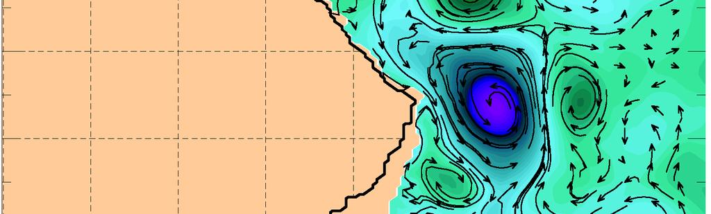
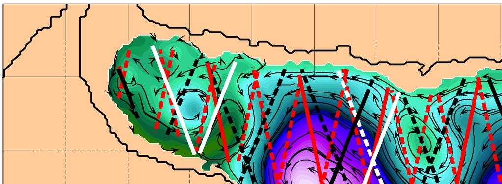
75 26 N Iran b c d e f g h i a N 22 N 15 1 Gulf of Oman 20 3 Arabian 20 N Peninsula N N 24 N 22 N 20 N 18 N 26 N 24 N 22 N 20 N 18 N 16 N 56 E 58 E 60 E 62 E 56 E 58 E 60 E 62 E 56 E 58 E 60 E 62 E (in cm) 30 cm/s Figure 2 75