IceWind final scientific report

Transcription

1 Downloaded from orbit.dtu.dk on: Dec 25, 2018 IceWind final scientific report Clausen, Niels-Erik; Giebel, Gregor Publication date: 2017 Document Version Publisher's PDF, also known as Version of record Link back to DTU Orbit Citation (APA): Clausen, N-E., & Giebel, G. (Eds.) (2017). IceWind final scientific report. DTU Wind Energy. DTU Wind Energy E, No General rights Copyright and moral rights for the publications made accessible in the public portal are retained by the authors and/or other copyright owners and it is a condition of accessing publications that users recognise and abide by the legal requirements associated with these rights. Users may download and print one copy of any publication from the public portal for the purpose of private study or research. You may not further distribute the material or use it for any profit-making activity or commercial gain You may freely distribute the URL identifying the publication in the public portal If you believe that this document breaches copyright please contact us providing details, and we will remove access to the work immediately and investigate your claim.

2 IceWind Improved forecast of wind, waves and icing

3 IceWind final scientic report Improved forecast of wind, wave and icing Report DTU Wind Energy E By Edited by Niels-Erik Clausen and Gregor Giebel Copyright: Reproduction of this publication in whole or in part must include the customary bibliographic citation, including author attribution, report title, etc. Published by: Department of Wind Energy, Frederiksborgvej 399 Web ISBN: ISBN: (electronic version)

4 Preface and acknowlegdement The present report is the final scientific report of the IceWind project, Improved forecast of wind, wave and icing The project involved more than 40 scientists from all five Nordic countries including three PhD students and one postdoc. The project participants acknowledge the financial support from Topforskningsinitiativet represented by Nordisk Energy Research as well as the support from the industry partners. Roskilde, October 2017 Niels-Erik Clausen and Gregor Giebel

5 Table of contents Table of contents... 1 Project participants... 3 Executive summary Introduction... 6 The Nordic Energy Context... 6 Problem description... 6 Project objectives... 7 How to read this report Wind turbine icing... 8 Introduction... 8 Ice modelling... 8 The use of observations to calculate icing... 8 The use of mesoscale models to calculate icing... 9 Makkonen ice accretion model... 9 Ice Mapping Long-term simulation of the icing climate for parts of Sweden and Finland Examples of icing maps for Nordic Countries Forecasting of icing Icing induced production losses Ice detection based on production losses Different methods to production loss forecasting Conclusions References List of publications Wind energy in Iceland The context and historical overview The wind climate on land Data used Wind climate The wind atlas Web interface More detailed assessment for select locations The offshore wind Data used Offshore wind climate Wind in the hydropower energy mix Conclusion References List of publications Improving and using weather, wave and production forecasts Introduction Wake loss modelling and interaction between wind farms Influence of weather model resolution on forecasting skill

6 Introduction Results Waves and vessel response Wave climate and weather windows Vessel behaviour as threshold parameter Calculation of vessel response Results Non-operable weather windows The effect of service vessel performance on wind turbine production RAM model Simulation of turbine and vessel Results Conclusion References List of publications Power and energy aspects Variability of wind power and the smoothing effect in Nordic countries Occurrence of low and high wind share situations in the Nordic countries Occurrence of storms in the Nordic electricity market area Case Study: The Dagmar storm and its implications for wind power Storm areas and durations in the Nordic countries statistical analysis Forecast errors and aggregation benefits in the Nordic electricity market area Wind power impacts on power system balancing Impacts of wind power variability on Nordic balancing power market Impacts of wind power forecast errors on Nordic balancing power market Impacts of icing on power system balancing Conclusions References Appendix A: Authors and affiliations

7 Project participants Project coordinator DTU Wind Energy (Niels Erik Clausen) Research partners DTU Wind Energy (Denmark) Kjeller Vindteknikk AS (Norway) Meteorologisk Institutt (Norway) Oceaneering Asset Integrity (Norway) VTT (Finland) Gotland University (Sweden) Weathertech Scandinavia (Sweden) subcontract to Gotland University Icelandic Met Office (Iceland) University of Iceland (Iceland) Industry partners Landsvirkjun (Iceland) Landsnet (Iceland) Vestas Wind Systems (Denmark) Statoil AS (Norway) Odfjell Wind AS (Norway) 3

8 Executive summary In order to address climate change and reduce the dependency of fossil fuels, the Nordic countries have set up targets to substitute fossil fuels for renewables. Hydro, biomass and wind energy are major contributors to the green transition on a Nordic scale. In the IceWind project we addressed some of the barriers for largescale integration of wind energy in the Nordic countries. A specifically Nordic challenge is ice formation on wind turbines that can cause a variety of problems for wind farms placed in cold climates. Ice forming on the turbine blades can cause production losses, increase the mechanical loads on turbine components, and falling ice can cause safety issues. In order to tackle these problems, better icing forecasting methods are needed. The IceWind project therefore developed an icing atlas for Sweden and Iceland based on long-term meteorological statistics. The development and validation of models for short-term forecast of icing has been based on numerical weather prediction models with advanced cloud, and hydrometeor parameterization schemes. It also developed an engineering tool for production loss calculation of large wind turbine installations in the northern latitudes. Four models have been tested on a controlled dataset that consists of weather model data and real production data collected from 15 different sites. Each model uses the same input weather data so the icing results can be compared to the observed icing and production loss models. Despite the design differences, the four models performed similarly. However, their performance did vary significantly across different wind farms, which suggests that there are local differences that are not well modelled, and that the models might not yet be general enough. The Icelandic power system is characterized by large amount of hydropower and geothermal power, and a constant high electricity demand. IceWind analysed the effect of integrating a wind farm in this system. Firstly, the wind power density in Iceland was mapped and the first ever wind atlas of Iceland was generated. Additionally, fourteen locations were selected for a more detailed study of the potential for development of wind energy. Furthermore, the wind resource off the coast of Iceland was mapped using satellite data. Finally, the interaction of wind and hydropower was examined in the context of the Icelandic power system. On the topic of power forecasts, it was shown that in many but not all cases it is advantageous to have a numerical simulation model with sufficiently high horizontal resolution. It was shown that even though computationally costly, Large Eddy Simulations provide better precision than the Weather and Forecasting Research (WRF) model. For Norway the wind forecasts from the global ECMWF model provided good results for most of the coastline. Further inland it is expected that high resolution WRF simulations will be superior if and when wind farms are built here. Further, IceWind contributed with a method that produced much more detailed estimates of the sea worthiness of different wind turbine service vessels and estimated the impact of the choice of service vessels can have on the power production of offshore wind turbines. This method reveals that choice of service vessels can have a significant impact on the availability and thus the production rate of an offshore wind farm, and that this impact is site specific. This was achieved by using detailed, historical wave spectra and wave response calculations for the service vessels. For the Nordic power system IceWind showed and quantified that a wide geographic distribution of wind power installations throughout the Nordic region has significant benefits for the power system on several 4

9 levels. The variability of the Nordic power system with high amount of renewable energy was investigated and the impact of forecasting errors on balancing needs was estimated. Firstly, the variability of the resulting power in-feed is relatively low, if the entire Nordic region is considered in comparison to a single country. This is especially true for the larger variations typically occurring at intermediate wind speeds. For example, the maximum step change from one hour to the next is nearly always below 5% of installed capacity for the aggregated Nordic area. Secondly, IceWind also showed that periods of low wind power production do not coincide with the highest demand on the power system, since low-wind periods are predominantly in summer and the highest demand in winter. During the 14 highest peak demands, we found that wind power produced at least 14% of the installed capacity. A particular challenge for the power system is a storm, which is so strong that it shuts off the turbines. While the largest storm in our database Dagmar that hit Norway, Sweden and Finland on 25 th December 2011, reduced the production from wind turbines in some regions to zero, it was not large enough to affect the whole Nordic area at once. Even in the affected regions Dagmar did not shut down wind power simultaneously, as the storm needed time to travel across the Nordic countries. A final benefit of a good geographical distribution is the smoothing of forecast errors. While smoothing on the national scale already decreases the Mean Absolute Error significantly, smoothing on the Nordic scale especially decreases the largest forecast errors. The effect of the decreased variability can also be seen in the power system. Even for wind power penetrations of 30%, the power system stays quite manageable, but intra-day correction of the largest forecast errors will be required. Finally, the effect of icing on the Nordic power system was studied. While initial results confirmed a limited local or regional impact on the power system of turbines shutting down due to icing, the larger impacts require more research, especially in ice removal from the affected parts of the turbines. 5

10 1 Introduction Niels-Erik Clausen The Nordic Energy Context Globally, wind energy is the fastest growing technology for electricity production with an average annual increase in cumulative installed capacity the last five years ( ) of 15%. In Europe for the last 16 years, wind energy has been the number one technology in the EU in terms of new capacity installed. At the end of 2016, the accumulated amount of installed wind power capacity in Europe was about 154 GW. In 2007 it was expected to reach 150 GW by the year That number was reached last year and the expectation is now more than 200 GW wind energy in Europe by The Nordic countries are contributing well to the green transition from fossil fuel based power generation to renewable energy sources. In the four Nordic countries the annual electricity consumption is 380 TWh of which 65% (2016) is from renewable energy most notably hydro, biomass and wind in that order. In Iceland electricity is 100% based on renewable energy. If we include heat and transport sectors the share of renewable energy is 38% of the primary energy supply (all five Nordic countries), while the largest single source of primary energy is oil. Problem description In order to address climate change and reduce further the dependency of fossil fuels the Nordic countries have set up targets to substitute fossil fuels for renewables. In the IceWind project we address some of the barriers for large-scale integration of wind energy in the Nordic countries. Icing is a problem for wind farms deployed at the northern latitudes. While there has been significant progress through the years in mitigating and avoiding the problem, forecasting of icing conditions has so far only received rudimentary attention. Likewise, there is no good method to estimate the probable losses due to ice of large-scale wind power installations in the Nordic countries. While currently, there are projects underway to map the North Sea and adjacent basins, the wind resource in the northern Atlantic between Iceland and Norway has received little attention so far. In Iceland expansion of the power system by building large new hydro power plants is not feasible for environmental reasons. On the other hand, the wind climate in Iceland is relatively good, but not well described. Furthermore, the wind resource has not been put into perspective with the grid data, in order to identify good feed-in points for wind farms. Furthermore, scheduling of a future combined hydro/geothermal/wind power system has so far not been properly investigated. A large-scale integration of wind power at a Nordic level calls for better forecasts. While forecasts for wind farms on land work quite well, there are still improvements to be implemented offshore. For example, currently the wave structure is not taken into account in the wind modelling offshore. Likewise, it is known 1 Clausen, N E et.al. Chapter 7 Wind power. In Climate & Energy Systems final report 2007 T. Thorsteinsson and H Björnsson (eds) ISBN Nordic Council of Ministers, Copenhagen. 6

11 that the wake structure inside the wind farms and behind the wind farms is dependent on the atmospheric stability, but currently this is not taken into account by the models. At the beginning of the IceWind project state-of-the-art was to build offshore wind farms in 200 MW units now (2017) a wind farm size of 500 MW or larger is common. Thus, the need for accuracy for forecasting of offshore wind farms has increased, as there is more power concentrated in one area. Project objectives The IceWind project address cold climate aspects and will include the production of an icing atlas for Sweden and one for Iceland based on long term meteorological statistics. The project will include development and validation of models for short-term forecast of icing by use of numerical weather prediction models and different cloud and hydrometeor parameterization schemes. The final objective is development of an engineering tool for production loss calculation of large wind turbine installations at northern latitudes. The project objectives include mapping of the wind resource of Iceland on land and including the sea near Iceland such that the following objectives can be achieved: Studies on the integration of hydro and wind power in Iceland. The objectives are to identify and enumerate potential future location scenarios for wind farms and identify location specific costs and benefit measures regarding investment and operations cost with timing and expansion assumptions for these scenarios. Furthermore, to estimate wind energy production when integrated with other resources and to identify transmission capacity restrictions and transmission loss measures for the range of locations and finally to design a short-term simulation system using optimization models. To facilitate large-scale integration of wind power project objectives include improved forecasting for 1) each wind farm, 2) the entire grid on energy production data and wake loss, 3) icing loss, and 4) offshore operation and cost-effective maintenance, optimizing choice of vessel types in different wave climates and providing specialized forecasts for accessibility. How to read this report Chapter 2 is describing the development of the tools for prediction of icing on wind turbines and tools to predict production losses. An icing atlas describing the average annual hours with icing conditions was developed for Sweden and Iceland. Chapter 3 is describing the assumptions and the work with development of the novel wind atlas of Iceland both on land and offshore. An initial analysis of system aspects of introducing wind energy in the Icelandic grid is presented. Chapter 4 is reporting two tasks: an analysis of forecasting of wind using Numerical Weather Prediction tools and an analysis of the influence the characteristics of the service vessel for an offshore wind farm have for the availability of the turbines and thus for the annual energy production. Chapter 5 analyses the benefits of geographical distribution of the wind farms over the Nordic region and the influence on variability of the power system. A special analysis is the analysis of the influence of a storm passing the Nordic region. 7

12 2 Wind turbine icing Halfdan Agustsson, Øyvind Byrkjedal, Neil Davis, Stefan Ivanell, Timo Karlsson, Stefan Söderberg. Introduction In cold climates, ice can form on any structure, and wind turbines are no exception. Wind turbine icing can cause a variety of problems for wind farms in these areas. Ice forming on the turbine blades can cause production losses, increase the mechanical loads on turbine components, and falling ice can cause safety issues for staff or the public. In order to tackle these problems, better icing forecasting methods are needed. Better icing forecasts can provide improved production forecasting of wind power in cold climates, and improve safety by warning of potential risks. However, forecasting alone is not enough and a better understanding of the effects of icing is also very important. The severity of icing has a relatively large year-to-year variance and icing conditions also change noticeably depending on local geography. Because of this variability, good modelling and forecasting methods are needed to evaluate the icing conditions at different locations. To provide an overview of the icing conditions in different places, various maps or ice atlases have been built. These ice maps illustrate the geographical variability in icing and can serve as a valuable first-step tool in evaluating icing conditions at different sites. The IceWind project approached the problems caused by wind turbine icing from two different viewpoints. Long term icing conditions were modelled to understand potential icing risks and the wind power potential in Nordic countries. Additionally short term forecasts and immediate effects of icing on wind turbines was studied to improve power production forecasts in icing conditions. In the IceWind project work towards the improvement of ice modelling, forecasting, and mapping was carried out by the project partners. Several ice maps for different Nordic countries were built during the project, and the impact of icing on wind turbine production was also studied. Ice modelling Icing of structures can be caused by either freezing rain or in-cloud icing. In-cloud icing happens when the temperature is below 0 C and the structure is covered in fog or reaches higher than the cloud base. In-cloud icing is significantly more common in Nordic countries. Because of that, this part of the IceWind project focused on modelling of in-cloud icing of wind turbines only. The use of observations to calculate icing To estimate how often icing occurs at a given site (icing hours), one can count the number of hours that have temperatures below 0 C and the presence of cloud water. The presence of clouds can be measured by several methods including ceilometers, which measure cloud height, or from visibility measurements. Harstveit [1] has developed a methodology that uses weather observations from airports to estimate icing conditions on exposed hills near the airport. This method uses observed cloud height and cloud coverage combed with modelled cloud water content and temperature profiles. 8

13 The use of mesoscale models to calculate icing Another definition of an icing hour was given in Byrkjedal & Berge [2]. Presenting one of the first icing atlases based on mesoscale modelling they defined an icing hour as an hour with an icing intensity larger than 10g/hr on the standard cylinder defined by ISO as a freely rotating cylinder with a 1-m length and 30- mm diameter. An ice amount of 10g on the ISO cylinder represent an ice layer of a thickness of 0.5 mm. The icing intensity calculation followed the Makkonen model [3] described below. The threshold of 10g/hr was imposed because the mesoscale model has a tendency to produce infinitesimally small amounts of cloud water (numerical noise) leading to infinitesimally thin layers of ice accretion that are not relevant for the resulting icing map. An alternative way to count icing hours from mesoscale model results is to use a threshold value on the liquid cloud water content from the model. Makkonen ice accretion model The following equation is included as an appendix to the ISO standard [4] for calculating icing rate dm dt w A V (1) where dm/dt is the icing rate on a standard cylindrical icing collector (defined by ISO as a cylinder of 1 m length and 30 mm diameter), w is the liquid water content, A is the collision area of the exposed object, V is the wind speed. α1, α2, and α3 are the collision efficiency, sticking efficiency, and accretion efficiency, respectively. Accumulated ice mass over time (1) gives M as the mass of ice on a standard cylindrical icing collector. Icing is calculated at a specific height, generally equivalent to the elevation of the turbine hub. The ice will remain on the turbine until it is removed by melting, sublimation, or mechanically as ice shedding. The time periods when ice is present on the cylinder, are defined as periods with instrumental icing, or in the case of a wind turbine rotor as rotor icing, while the period when conditions lead to ice growth are called meteorological icing (see Figure 1, p. 6). We have defined the periods with instrumental icing as the periods when the ice mass, M, exceeds 10 g/m. During instrumental icing periods, wind speed measurements can also be affected by icing, and the turbines will most often experience a reduction in power production. 9

14 FIGURE 1: ICING CYCLE OF A WIND TURBINE. Ice Mapping Maps of icing can be created using either the observational or meso-scale model approach. However, both of these approaches have limitations when trying to create a map showing the geographical distribution of icing. The amount of icing and the icing frequency depends mostly on the air temperature and the availability of liquid water. Due to the lapse rate, reduction of temperature with height, the number of days with temperatures below the freezing point increases at higher elevations. Since the saturation vapour pressure of water decreases with decreasing air temperature, higher elevations also are more likely to have more condensation and therefore more liquid water available to form ice. For observational icing, these small scale differences can make it hard to interpolate icing data collected at one site to another site. Additionally for wind turbine related icing, the sensors typically used for detecting ice growth are in different conditions than the tips of the turbine blades that impact power production the most. Therefore, models are often relied upon for making icing maps. Data from a mesoscale model already has the spatial weather information needed to create a map. However, the models are limited by their parameterizations and the relatively coarse horizontal and vertical resolution able to be used. Formation of cloud particles and clouds is the most important parameter for icing models and at the same time one of the areas where the models are most uncertain. This is because clouds are sub-grid scale processes in a mesoscale model, and their accurate modelling depends on the model capturing many other processes realistically. Additionally, mesoscale models have a relatively coarse topography due to the horizontal resolution of the model. This coarse terrain will typically underestimate the elevation of hills and overestimate the elevation for valleys, leading to a smoothed topography. 10

15 Long-term simulation of the icing climate for parts of Sweden and Finland Within the IceWind project, the long-term variability of the icing climate was studied. Icing maps were produced and time series were analysed for selected sites. As basis for the study, data from the mesoscale model WRF [11] was used. ERA Interim, a reanalysis dataset provided by the ECMWF, was used as initial and lateral boundary conditions. To be able to model supercooled liquid cloud water, a suitable microphysics parameterization scheme has to be used. In this study, the Thompson et al. (2008) scheme was applied [10]. The model was run for 34 years, , with both a 3km x 3km and a 9km x 9km horizontal grid resolution. A shorter period, , was run with a 1km x 1km horizontal grid resolution. The use of different resolutions allowed for a comparison between modelled icing climates at different model resolutions. While it is common to adjust the model parameters to the observed terrain, to account for the unresolved topography, this was not done in this study since the objective was to study the differences in icing climates due to different model grid resolutions and time periods. The icing maps show number of hours with active icing per year (5-years and 34-years means) for all resolutions. Active icing is here defined as an hour with icing intensity of more than 10g/h on the ISO cylinder. Ice maps for a portion of northern Sweden and Finland are available in Söderberg & Baltscheffsky [12] and in pdf format on request from WeatherTech. In the report, an analysis of the long-term variability in production losses due to icing is also included. Examples of icing maps for Nordic Countries Norway Kjeller Vindteknikk (KVT) developed an icing map for Norway in 2009 [5]. The map was developed using data from the meso-scale model WRF. The work was performed as part of A wind map for Norway funded by the Norwegian Water Resource and Energy Directorate (NVE). The map shows the number of icing hours per year, where an icing hour is defined as an hour with an icing intensity (active icing) of more than 10g/h on the standard ISO cylinder. The mesoscale simulations that formed the basis of this map were performed with a horizontal resolution of 1 km x 1 km, for a single model year. The map was corrected towards a normal year (defined as the average of the years ) using a coarser resolution WRF simulation. A height adjustment function was used to incorporate high resolution topography (50 m x 50 m) and correct for the smoothed model terrain. Validation of the map was carried out by comparing the number of icing hours at different height levels with icing estimated based on cloud observations from METAR data for two regions in Norway [1], [2]. The validation showed that the icing map has a tendency of over predicting the number of icing hours for areas with elevation lower than m. a. s. l. The icing map is available as a pdf mapbook or as GIS readable data. 11

16 Sweden An icing map for Sweden (see Figure 2, p. 8) was publicly released by KVT in 2012 [6]. The methodology used for this atlas was similar to the Norwegian icing atlas, with a few improvements. Like the Norwegian icing atlas, the Swedish icing atlas was based on one year of WRF model simulations with 1 km x 1 km horizontal resolution, and was long term corrected using a coarser model result for the years The simulation for Sweden used a more sophisticated microphysics parameterization scheme than the Norwegian icing atlas [7]. The microphysics parameterization scheme is the part of the model that describes the cloud formation and precipitation processes. The implementation of the Makkonen [3] model and the height correction algorithms were also changed in the Swedish icing atlas compared to the Norwegian one. No systematic validation of this icing map has been carried out. The icing map is available as a pdf mapbook or as GIS readable data. 12

17 FIGURE 2: ICING MAP OF SWEDEN

18 Finland The Finnish Icing Atlas (see Figure 3, p.10) was constructed in collaboration between VTT and the Finnish Meteorological Institute (FMI). FMI carried out the weather and ice modelling using the AROME weather model, and an icing model based on the ISO standard [4]. The icing model was used to calculate the accumulated ice mass on a stationary cylinder for different weather conditions [8]. To provide an estimate of energy production losses under different icing conditions, VTT modelled the power performance behaviour of a wind turbine under icing conditions. Part of this modelling work was done under the IceWind project [9]. Three rime ice cases were selected that had meteorological conditions typical for the Finnish climate. The conditions were the same for each case. The lengths of the icing events were varied to represent the beginning of icing, a short icing event, and a long icing event. Thus, three different ice masses accreted on a wind turbine blade were simulated using the VTT developed TURBICE tool [27]. The aerodynamic properties of the iced profiles were modelled using computational fluid dynamics (CFD) with the ANSYS FLUENT flow solver. The lift and drag coefficients were evaluated as a function of an angle of attack, and small scale surface roughness effects on the drag coefficient were determined analytically. Finally, power curves were generated with FAST turbine simulation software [28] for clean wind turbine blades and for blades with each of the three different ice accretions. The results of this study were used in the Finnish Icing Atlas (2012), where time dependent numerical weather simulations were carried out to calculate both icing conditions and energy production losses. The Finnish icing atlas can be found at 14

19 FIGURE 3: EXAMPLE VIEW FROM FINNISH ICING ATLAS PRESENTING ESTIMATED PRODUCTION LOSSES AT 100 M ABOVE GROUND

20 Iceland Studies of atmospheric icing in Iceland go back over 40 years and have their roots in the need for mapping icing loads at the sites of planned power lines across the Icelandic highlands [13]. In fact, since the first overhead conductors and telephone wires in the early 20th century, atmospheric icing has been a serious problem, frequently faced by line operators. Although infrequent, wet-snow accretion regularly causes problems and damage in the low-lands as well as in the mountains. In-cloud icing rarely occurs below approximately 300 m, but is frequent above that elevation in all parts of Iceland, leading to large problems if it was not accounted for when dimensioning the electricity transmission system, telecommunication towers, and similar structures. Consequently, most studies on atmospheric icing in Iceland have focussed on accretion on overhead wires and the needs of the transmission and distribution system operators. Studies of icing on overhead conductors in Iceland benefit from a unique database composed of: a) Reports of all observed icing events on overhead wires since the early 20th century, often with the icing diameter and even mass measured as well [14] and b) data from approx. 60 test spans measuring icing throughout Iceland. The first span was erected in 1972 and since 1989 the spans have gradually been modified to measure the icing load in real time instead of only annual maxima [15]. Only recently, and in connection with the first large scale wind turbines in Iceland has there been growing interest in icing related to wind energy and turbines, but no relevant observational data is available. Within IceWind an icing atlas has been made for Iceland. The atlas treats wet-snow and in-cloud ice accretion separately. Taking into account the atmospheric icing framework in Iceland, the focus is mainly on overhead conductors, but part of the atlas focuses on the needs of the wind energy industry. In this context, it should be noted that the needs of the line operators and the wind energy industry are very different. Line operators need icing forecasts and maximum loads that can be expected for a given period, say a 50-year icing load, while the wind industry's main needs lie in forecasts and estimates of the frequency icing events, preferably broken down into different intensities. Within the icing atlas, ice accretion is parameterized based on the frequently used cylindrical model of Makkonen [4]. The atmospheric data needed as input is a part of the RÁV-project [16] and was prepared with the state-of-the-art WRF atmospheric model [17]. The WRF-model was initialized with analysis data from the ECMWF, and used to simulate the state of the atmosphere above Iceland at a horizontal resolution of 3 km for A simulation at 9 km resolution run from was used for comparison. The model used 40 vertical layers and the Thompson microphysics scheme [10] and [18]. This setup provides the necessary parameters and detail of atmospheric water distribution needed to calculate both wet-snow and in-cloud accretion. The ETA planetary boundary layer scheme [19] is the second most relevant parameterization scheme employed, since atmospheric stability and uplift, and thereby atmospheric water and precipitation distributions, are strongly linked to the microphysics scheme and the PBL scheme, as well as other factors not mentioned here. Furthermore, data simulated with 55 levels in the vertical and at a resolution of 9, 3 and 1 km from over 10 cases (longest case covers the winter of ) of wet-snow and in-cloud accretion have furthermore been used in development and tuning of the model. Since the orography is smoothed considerably at the resolution of the atmospheric model, the atmospheric data is interpolated upwards at each grid point to the true elevation of the surface. As it is not relevant for the study, i.e. we seek an upper bound on maximum icing loads, no attempt is made to correct for overestimated terrain elevation. 16

21 Separate maps are prepared for in-cloud icing and wet-snow accretion near the surface. Maximum ice loads are prepared for a vertical cylinder, as well as for four different directions of a horizontal cylinder, i.e. taking wind direction into account (0, 45, 90 and 135 ). Finally, maps are prepared for two different in-cloud accretion frequencies at 50 m above ground level. Methods to forecast icing in real time have also been prepared and are based on same models and presented in the same way as the icing maps. FIGURE 4: MAXIMUM SIMULATED ICE LOAD AT SURFACE. Forecasting of icing While ice maps are helpful for determining areas with likely icing impacts, icing forecasts are needed for the day-to-day operation of wind farms that are at risk for icing. The forecast of icing for wind energy is tied closely to the icing induced production losses that will be described in the next chapter. Providing accurate icing forecasts allows site operators to better estimate their day-ahead power production, avoid costly over predictions, and are used for ensuring the health and safety of the public and onsite workers. Forecasts of icing rely on mesoscale models and techniques similar to those described in section 2.2. Because of the time dependent nature of forecasts, simplified icing models are required due to their computational efficiency. This may also impact the selection of parameterization schemes used in the mesoscale model simulations. 17

22 FIGURE 5: FREQUENCY OF A GIVEN ACCRETION INTENSITY AT 50 ABOVE SURFACE (MISSPELLED AS 100M IN THE TEXT). It has been found that icing forecasts do a reasonable job of capturing the onset of icing, even with different mesoscale and icing models. However, the models currently differ significantly in the timing of the ice removal [20]. The modelled ice tends to remain on the turbine for longer than is evidenced by the observed power production. Therefore, using the observed power production to aid in determining the end of an icing event will improve the model forecasts. In table 1, an icing model is validated at three different locations [26]. TABLE 1: VALIDATION OF FORECASTING OF INSTRUMENTAL ICING ON THREE SITES [26]. Site 1 Site 2 Site 3 Ratio of time when ice is detected 21 % 13 % 10 % False alarm ratio 2.4 % 2.9 % 5.6 % Probability of detection 73 % 68 % 81 % It has also been found that the rate of ice growth is significantly different on a standard cylinder compared to a wind turbine blade. This difference is largely due to the rotation of the turbine blades, which increases the relative droplet velocity [21]. Therefore, when modelling icing impacts on wind turbines, it is important to take 18

23 the rotational speed into account, both for ice accretion and ice ablation. To forecast the impact of icing on power production, the ice forecasts are passed to production forecast models that account for the impact of ice on wind farm power performance. These models will be discussed below in page 16. Icing induced production losses Icing of a wind turbine can decrease the power production significantly due to changes in blade aerodynamics. As ice builds-up on the blade, it changes the blade s aerodynamic properties, decreasing lift and increasing drag. This in turn decreases the turbine s power production. The impact of icing on the overall power production depends on multiple factors, including type, shape, and mass of the ice, all of which vary for different icing events. In addition to differences in ice shape and type, differences in local geography, site conditions, turbine type, and control strategies all affect the real-world observed production loss caused by ice accretion on the blades. Due to these uncertainties, statistical methods are used in order to model the icing induced production losses. Production loss models can be used either as part of a wind power forecasting system or as a tool to estimate power production at a cold climate site. The basic structure of such a model is illustrated below (see Figure 6): FIGURE 6: EXAMPLE FLOWCHART OF A POWER PRODUCTION SYSTEM THAT INCLUDES AN ICING COMPONENT [22]. 19

24 Ice detection based on production losses Because icing leads to production losses, it can be used to detect icing by examining the power production of operating turbines. This can be done by monitoring when the output power of a wind turbine drops below a predetermined threshold. The easiest method for setting the threshold is to use a percentage of the manufacturer power curve. The most common percentages being between 85% and 75% of the reference power curve. Other approach is to build the threshold curve from observations. This can be done either using standard deviation or by using a quantile of the data. Building the threshold limit from observations requires first building a clean reference dataset. This dataset needs to be completely ice free and only include periods when the turbines are operating normally. The best way to do this is to filter the observations based on ambient temperature. It is important to note that this temperature should not be set to 0 C, since ice will often still be on the blade during such conditions. It has been found that a value of 3 to 5 C is usually needed to ensure an ice-free dataset [23]. After the reference dataset is built, it is binned according to wind speed a threshold limit is calculated for each bin. When using the standard deviation method a standard deviation of the power is calculated for each bin. Then the threshold limit is calculated for each wind speed based on the standard deviation of the power in that bin. The quantile method is similar, but simply sets the limit at a prescribed quantile, for example the threshold limit could be set so that 10% of the clean data is below that value in each bin. A comparison of different methods for setting these limits can be found in [23]. The biggest issue when using past production data to create ice detection threshold limits is dealing with outliers in the production data. Because of the outliers, the more robust quantile method is often more reliable than the standard deviation approach, and can allow for more data to be retained during the cleaning phase. Once the threshold curve has been determined, icing can be detected from production data by demanding that the output power is below the threshold limit and ambient temperature is low enough. Other conditions can be added here to increase the robustness of the detection methods. One common approach is to require that the produced power stays below the threshold limit for a certain amount of time (e.g. 30 minutes to an hour) before issuing an icing alarm. This allows for short dips below the production limit that are likely not icing to be excluded from the detection algorithm. Different methods to production loss forecasting Four different approaches to production loss modelling from different project partners were tested to see how these different approaches to the same problem compare, and to find ways to improve the models by understanding which approaches produced better results. In every model, the general approach was similar: the production loss model was built as a stand-alone unit that uses input data from a numerical weather model to estimate the impact of icing in the power production. All models use different kinds of statistical models to describe the effects of ice on wind turbine power production. The VTT and DTU models were developed in the IceWind project. The two other models were created by project partners in previous projects. However, they were improved over the course of the IceWind project. A summary of the models and the comparison results will be presented here, the full results of the comparison are presented in [24]. 20

25 DTU The DTU production loss modelling approach used the DTU IceBlade ice model described [25]. The IceBlade model used a modified version of the standard Makkonen ice model to model the ice build-up. In order to estimate the total ice mass, IceBlade includes algorithms for three methods of ice ablation: there are separate models for sublimation and erosion, and a total shedding condition that specifies that all ice falls from the turbine when the temperature is above 0 C. The results from IceBlade were used to fit a statistical icing power loss model. The power loss model is a hierarchical model consisting of a decision tree and two different generalized additive models (GAM). The hierarchical approach was chosen so different models could be used for iced and non-iced data points. The production loss model uses inputs from both a numerical weather model and an icing model to improve accuracy. The model was fit using real production data to describe the production losses. VTT The VTT model was built using statistical methods based on production data only [21]. This approach was used in order to build a model that is as simple as possible (requiring as few inputs as possible), portable (not reliant on a specific weather prediction model or a specific production forecast model), and accurate enough to produce useful results. When building the model, the first step was to identify the variables that have an effect on the severity of the icing incident. Severity here means the magnitude of production loss. After analysing several different datasets from multiple sites, wind speed and the length of the icing period were chosen as inputs to the model. The model was built based on production data by first identifying the icing events that have occurred at a site. After the icing events were identified, a three-dimensional power curve was fit on this data based on production loss during the event, event length, and wind speed. KVT Kjeller Vindteknikk has developed a production loss model that uses the principle of a two parameter, wind speed and ice load, three-dimensional power curve based on wind tunnel experiments. Ice load is defined as the total ice mass built up on a standard cylinder. The power curve used in this study was created based on operational data from three wind parks in Sweden. To calculate the total ice mass, ice removal needed to be included in the KVT model. The KVT ice model includes algorithms for melting and sublimation, as well as a term that represents the erosion of small pieces of ice. WeatherTech WICE model The WeatherTech production loss model (WICE) includes a physical module for modelling ice accretion and ice ablation on a simplified wind turbine blade, and a statistical module that relates the modelled ice and the properties of the atmosphere to the performance of the turbine. An artificial neural network is used to relate the ice model to production losses. 21

26 Comparison of the different approaches The four models were tested on a controlled dataset that consisted of a weather model data and real production data collected from 15 different sites. Each model used the same input weather data so the results would compare the icing and production loss models and not the weather models. Since the VTT approach does not rely on a specific ice model, the icing forecast from DTU s IceBlade model was used as an input for the VTT model. The four production loss models used in this study vary greatly in their inputs and design. Two of the models fit only one additional term from an icing model to the standard power curve of the wind park, while the other two models combined many different inputs from the physical meteorological and ice models. Despite the differences, three of the four production loss models produced very similar results. This suggests that the model used for estimating the production loss is not as important as the inputs from the weather and icing models. Despite the design differences, the different models performed similarly. However, their performance did vary significantly across different wind parks, which suggests that there are significant local differences, and that the models might not yet be general enough. Additionally, all models tended to do worse at parks with less icing. Conclusions In the IceWind project, icing conditions and the impact of icing on wind power production in the Nordic countries were modelled using several different approaches. The results from the Icing models showed that local variations in geography and climate do affect the icing conditions noticeably. Also, the severity of icing can fluctuate significantly from year to year. These results applied to all countries studied in this project. The IceWind project partners also found out that the effects icing has on wind turbines can be modelled using statistical methods using several different approaches. These production loss methods combined with short term icing forecasts were shown to improve production forecasts in areas with icing climates. 22

27 References [1] Harstveit, K. (2009): Using Metar-Data to Calculate In-Cloud Icing on a Mountain Site near by the Airport IWAIS XIII, Andermatt, September 8 to 11, [2] Byrkjedal, Ø. & E. Berge (2008): The Use of WRF for Wind Resource Mapping in Norway, WRF User Workshop, Boulder, June [3] Makkonen, L., (2000): Models for the growth of rime, glaze, icicles and wet snow on structures. Philosophical Transactions of the Royal Society A: Mathematical, Physical and Engineering Sciences, 358 (1776), , doi: /rsta / /rsta [4] ISO (2001): Atmospheric icing of structures. ISO 12494, Geneva, Switzerland, 56. [5] Byrkjedal, Ø. & E. Åkervik (2009): Vindkart for Norge, NVE oppdragsrapport A9-09, in Norwegian. pporta9-09.pdf [6] Byrkjedal, Ø. (2012): Icing map for Sweden, KVT report KVT/ØB/2012/R076. [7] Thompson, G., P.R. Field, W.D. Hall & R. Rasmussen (2006): A new bulk Microphysical Parameterization Scheme for WRF (and MM5). [8] Tammelin, B., T. Vihma, E. Atlaskin, J. Badger, C. Fortelius, H. Gregow, M. Horttanainen, R. Hyvönen, J. Kilpinen, J. Latikka, K. Ljungberg, N.G. Mortensen, S. Niemelä, K. Ruosteenoja, K. Salonen, I. Suomi & A. Venäläinen (2011): Production of the Finnish Wind Atlas. Wind Energy. Research article. [Cited ]. DOI: /we.517. [9] Turkia, V., S. Huttunen & T. Wallenius (2013): Method for estimating wind turbine production losses due to icing. VTT Technology 114. VTT, Espoo. [10] Thompson, G., P. R. Field, R. M. Rasmussen & W. D. Hall (2008): Explicit forecasts of winter precipitation using an improved bulk microphysics scheme. Part II: Implementation of a new snow parameterization. Mon. Wea. Rev., 136, [11] Skamarock, W. C., J. B. Klemp, J. Dudhia, D. M. Gill, M. Duda, X.-Y. Huang, W. Wang & J. G. Powers (2008): A Description of the Advanced Research WRF Version 3. NCAR Technical Note. [12] Söderberg, S. & M. Baltscheffsky (2015): Long-term mapping of icing for parts of Sweden and Finland, IceWind WP1 Technical Note. [13] Sigurðsson, F. H. (1971): Ísingarhætta og háspennulína yfir hálendið, Veðrið 16 (2), p

28 [14] Ísaksson, S. P., Á. J. Elíasson & E. Thorsteins (1998): Icing Database Acquisition and registration of data. Proc. Eighth Int. Workshop on Atmospheric Icing of Structures (IWAIS), Reykjavík, Iceland, p [15] Elíasson, Á. J. & E. Thorsteins (2007): Ice loadmeasurements in test spans for 30 years. Proc. 12 th Int. Workshop on Atmospheric Icing of Structures (IWAIS), Yokohama, Japan, Japanese Society of Snow and Ice, 6 pp. [16] Rögnvaldsson Ó., H. Ágústsson & H. Ólafsson (2009): Stöðuskýrsla vegna þriðja árs RÁVandar verkefnisins. ftp://ftp.betravedur.is/pub/publications/rav-stoduskyrsla2009.pdf [17] Skamarock W.C., J. B. Klemp, J. Dudhia, D. O.Gill, D.M. Barker, M. G. Duda, X.-Y. Huang, W. Wang & J. G. Powers (2008): A description of the advanced research WRF version 3, Technical Note TN- 475+STR. NCAR: Boulder, CO. [18] Thompson, G., R. Rasmussen & K. Manning (2004): Explicit forecasts of winter precipitation using an improved bulk microphysics scheme. Part I: Description and sensitivity analysis [19] Janjic, Z. I. (2002): Nonsingular implementation of the Mellor Yamada level 2.5 scheme in the NCEP Meso model. NCEP Office Note 437, 61 pp. [20] McDonough (2014): Ice Intercomparison. Winterwind, Sundsvall, Sweden. [21] Davis, N., A. N. Hahmann, N.-E. Clausen & M. Žagar (2014): Forecast of Icing Events at a Wind Farm in Sweden. Journal of Applied Meteorology and Climatology Feb 2014; 53(2): , doi: /jamc-d [22] Karlsson T., V. Turkia & T. Wallenius (2013): Icing production loss module for wind power forecasting system. Technical Report, VTT Technical Research Centre of Finland, Espoo, Finland. [23] Davis, N., Ø. Byrkjedal, A. N. Hahmann, N.-E. Clausen & M. Žagar (2016): Ice detection on wind turbines using the observed power curve. Wind Energ., 19: doi: /we [24] Davis, N., A. N. Hahmann, N.-E. Clausen, M. Žagar, Ø. Byrkjedal, T. Karlsson, V. Turkia, T. Wallenius, M. Baltscheffsky & S. Söderberg (2014): Inter--comparison of icing production loss models. Winterwind, Sundsvall, Sweden; 02/2014. [25] Davis, N., P. Pinson, A. N. Hahmann, N.-E. Clausen & M. Žagar (2015): Identifying and characterizing the impact of turbine icing on wind farm power generation. Wind Energ., doi: /we [26] Byrkjedal, Ø., H. van der Velde & B. E. K. Nygaard (2015): Validation of icing and wind power forecasts at cold climate sites, Presentation at Winterwind. 24

29 [27] Makkonen, L., T. Laakso, M. Marjaniemi & K. Finstad (2001): Modelling and prevention of ice accretion on wind turbines, Wind Engineering 25(1), [28] National Renewable Energy Laboratory: NWTC Information Portal (FAST v7). last modified 19-March-2015, Accessed 14-August List of publications Turkia, V., S. Huttunen & T. Wallenius (2013): Method for estimating wind turbine production losses due to icing. VTT Technology 114. VTT, Espoo. Karlsson, T., V. Turkia & T. Wallenius (2013): Icing production loss module for wind power forecasting system. Technical Report, VTT Technical Research Centre of Finland, Espoo, Finland. Karlsson, T., V. Turkia, T. Wallenius & J. Miettinen (2014): Production Loss estimation for wind power forecasting Presentation at Winterwind. Davis, N. (2014): Icing Impacts on Wind Energy Production. 10/2014, Degree: PhD, Supervisor: A. N. Hahmann, N.-E. Clausen, M. Žagar. Davis, N., A. N. Hahmann, N.-C. Clausen & M. Žagar (2014): Forecast of Icing Events at a Wind Farm in Sweden. Journal of Applied Meteorology and Climatology 02/2014; 53(2): DOI: /JAMC-D Davis, N., P. Pinson, A. N. Hahmann, N.-E. Clausen & M. Žagar (2002): Identifying and characterizing the impact of turbine icing on wind farm power generation. Wind Energ., doi: /we Davis, N., Ø. Brykjedal, A. N. Hahmann, N.-E. Clausen & M. Žagar (2002): Ice detection on wind turbines using the observed power curve. Wind Energ., 19: doi: /we Davis, N. (2014): Modeling of icing impacts on wind parks. Danish Research Consortium for Wind Energy R&D Conference, Herning, Denmark; 03/2014. Davis, N., A. N. Hahmann, N.-E. Clausen, M. Žagar, Ø. Byrkjedal, T. Karlsson, V. Turkia, T. Wallenius, M. Baltscheffsky & S. Söderberg (2014): Inter--comparison of icing production loss models. Winterwind, Sundsvall, Sweden; 02/2014. Davis, N., A. N. Hahmann, N.-E. Clausen, M. Žagar & P. Pinson (2013): Forecasting Production Losses by Applying Icing Models to Wind Turbine Blades. The 15th International Workshop on Atmospheric Icing of Structures, St. John's, Newfoundland and Labrador, Canda; 09/2013. Davis, N. (2013): Icing on Wind Turbines. Onshore O&M Forum, Hamburg, Germany; 06/2013. Davis, N., A. N. Hahmann, N.-E. Clausen, M. Žagar & P. Pinson (2013): Forecasting Production losses at a Swedish Wind Farm. Winterwind, Östersund, Sweden; 02/

30 Davis, N., Hahmann, Andrea, Clausen, Niels-Erik Žagar, Mark: Evaluation of WRF Microphysical Schemes for use in forecasting Wind Turbine Icing. 13th Annual WRF Users' Workshop, Boulder, CO, USA; 06/2012. Davis, Neil N., A. N. Hahmann, N.-E. Clausen & M. Žagar (2012): Forecasting Turbine Icing Events. European Wind Energy Agency, Copenhagen, Denmark; 04/2012. Davis, N., A. N. Hahmann, N.-E. Clausen & M. Žagar (2012): WRF Sensitivity Analysis of Boundary Layer Clouds During the Cold Season. Winterwind, Skelefteå, Sweden; 02/2012. Byrkjedal, Ø., H. van der Velde, B. E. K. Nygaard (2015): Validation of icing and wind power forecasts at cold climate sites, Presentation at Winterwind. Byrkjedal, Ø., R. E. Bredesen, A. L. Løvholm (2014): Operational forecasting of icing and wind power at cold climate sites, Presentation at Winterwind. Byrkjedal, Ø. (2013): Icing map of Sweden, presentation at Winterwind. Byrkjedal, Ø. (2013): On the uncertainty in the AEP estimates for wind farms in cold climate, presentation at Winterwind. Byrkjedal, Ø. (2012): Mapping of icing in Sweden On the influence from icing on wind energy producion, presentation at Winterwind. Byrkjedal, Ø. (2012): The benefits of forecasting icing on wind energy production, Poster presentation at Winterwind. Nygaard, B. E. K., H. Ágústsson & K. Somfalvi-Tóth (2013): Modeling wet snow accretion on power lines: Improvements to previous methods using 50 years of observations, Journal of Applied Meteorology and Climatology, 52 (10), Elíasson, Á. H., Á. J. Hannesson, M. Guðmundur & E. Thorsteins (2013): Modeling wet-snow accretion -- Comparison of cylindrical models to field measurements, pp th International Workshop on Atmospheric Icing of Structures, Canada. Elíasson, Á. H., Á. J. Hannesson & M. Guðmundur (2013): Wet-snow Accumulation A Study of two severe Events in complex Terrain in Iceland, pp th International Workshop on Atmospheric Icing of Structures, Canada. Elíasson, Á. J., H. Ágústsson, Ó. Rögnvaldsson & E. Thorsteins (2012): Hermun ísingaráhleðslu á loftlínur (en. Simulation ice accretion on overhead powerlines). Árbók verkfræðinga- og tæknifræðingafélags Íslands, p , ISSN: Ágústsson, H. (2014:) Öfgar í veðri - Ísing (e. Extremes in weather - Atmospheric icing). Short contribution to the annual report of the Icelandic Meteorological Office, February

31 Elíasson, Á. J., E. Þorsteins, H. Ágústsson & Ó. Rögnvaldsson (2011): Comparison between simulations and measurements of in-cloud icing in test spans, p. 7. (International workshop on atmospheric Icing on structures), China. 27

32 3 Wind energy in Iceland Halldór Björnsson, Nikolai Nawri, Charlotte Bay Hasager, Gunnar Geir Pétursson, Guðrún Nína Petersen, Birgitte Furevik, Úlfar Linnet, Kristján Jónasson, Merete Badger, Andrea N. Hahmann and Niels-Erik Clausen. The context and historical overview The energy sector in Iceland has an unusually high share of renewable energy in the total primary energy budget. Geothermal energy provides about two thirds of the total energy budget, primarily for space heating, with about 90% of all households heated with geothermal water. Almost all electricity used in Iceland derives from renewables, with hydropower supplying three fourths of the production, and geothermal power plants producing the rest. Iceland has the world s highest energy production per capita (53.16 MWh/capita in 2012) but more than 80% of the electricity produced is used by power intensive industries. The Icelandic energy system is isolated from that of Europe, and the fact that a few industrial users are responsible for most of the electricity demand, means that the demand is quite stable. Due to Iceland's position in the North Atlantic storm track, the wind climate might a-priory be expected to be favourable for wind power production. Indeed, large scale global comparisons tend to support this. Furthermore, one aspect of hydropower in Iceland is that the streamflow in rivers tends to exhibit a large annual variation, with larger flow during summer than in winter. Since the annual cycle of wind in Iceland has the opposite phase, with stronger winds in winter than in summer, wind power can potentially fit well with in a hydropower dominated system. Nevertheless, detailed research into the wind power potential of Iceland is quite recent, with the first limited resource assessment published in 2007 [29]. The IceWind project was therefore groundbreaking, in that one of the work packages was focused on wind resource assessment, leading to the production of a Wind Atlas for Iceland. The successful conclusion of this task was a major step forward in obtaining an overview of the wind resource in Iceland, and the atlas is a tool that more localized and detailed assessments can be based upon. This chapter discusses the wind climate of Iceland, and the methodology used to calculate the Wind Atlas. It also presents the web interface to the atlas. Additionally, the IceWind project examined the offshore wind climate, and results from that analysis will also be presented. We finish with an examination of the windhydropower mix followed by conclusions. The wind climate on land One of the main tasks in the work package that focused on wind resource assessment for Iceland was the generation of a wind atlas. A prerequisite for the atlas was to map the wind climate of Iceland. The first parts of this section discuss the construction of the data base used for this task, and present maps of the winds in Iceland. (See [30] for a more detailed discussion). 28

33 Data used In comparison with measurements of temperature and precipitation, wind measurements in Iceland have a relatively short history. Following sporadic attempts of measuring winds in Reykjavik in the 1930s, and the installation of two anemometers in Reykjavik and Keflavik after World War 2, it was not until the latter part of the 20th Century, that a network of anemometers was established. Until the late seventies the number of stations in this network was less than 15, increasing to up to 23 in the late eighties. Following the mid-nineties, a revolution began in the measurement of wind strength and direction. This was precipitated by the installation of automatic weather stations, the oldest in continuous operation dating from 1994, and with the network having expanded to almost 260 stations in Of these stations, the Icelandic Meteorological Office (IMO) operates 120, the road services 86, and Landsvirkjun (the national power company) 16 stations. The remaining stations were operated by other power companies, harbours, and various smaller entities. This network does not provide completely comparable data. The road services place the anemometers at 6-7 m above ground level (AGL), while IMO, Landsvirkjun, and most others use the standard 10 m AGL. Furthermore, some of the smaller operators do not maintain a high quality standard of measurements. Despite this, currently the situation for wind measurements in Iceland is a vast improvement over the situation a few decades ago. For the period , the anemometer network had 145 stations with high quality data, consisting of 10 minute average wind measurements and wind gusts. Despite the station network being fairly well distributed over Iceland, the orography of Iceland is sufficiently complex that interpolating the station data to a regular horizontal grid does not yield satisfactory results. To overcome this, data from WRF simulations were used to generate a background field that was then adjusted using the station data, resulting in an estimate of the surface wind fields over Iceland. The simulated data used for this study was obtained from the Institute for Meteorological Research in Iceland, and was calculated as part of the RÁV project a joint project between several Icelandic institutions. The RÁV model runs were produced with the mesoscale Weather Research and Forecasting (WRF) [31] and covered the period 1994 to In order to match the best observations and simulations, the main analysis here was limited to the four year period 2005 to The WRF simulations were performed in three nested horizontal domains, all approximately centred around Iceland. The innermost domain had a spatial resolution of 3 km, and the only landmass in it was Iceland. The initial and boundary conditions for the WRF model simulations were determined by 6-hourly operational analyses obtained from the European Centre for Medium-Range Weather Forecasts (ECMWF), valid at 00, 06, 12, and 18 UTC (which is local time in Iceland throughout the year). After initialisation of the model run, this data was only applied at the boundaries of the largest domain (which had a resolution of 27 km). Calculations in this domain were then used to update the boundary conditions for the intermediate domain (which had a resolution of 9 km). The intermediate domain was then used in turn to update the innermost (3km grid) domain. The WRF results were biased in that winds were too weak over land, but these biases where removed using observations to scale the WRF generated wind, resulting in an adjusted wind fields. 29

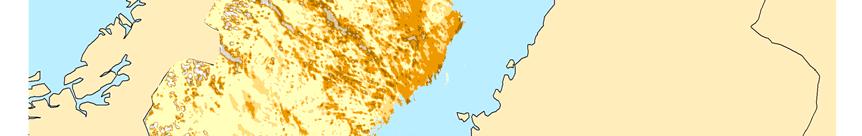
34 FIGURE 7: MAP OF ICELAND SHOWING THE LOCATIONS OF SITES CHOSEN FOR FURTHER STUDY. Wind climate Annual averages and winter (DJF) and summer (JJA) averages of adjusted wind speeds at 50 and 100 magl are shown in Figure 8. The spatial variability of wind speed strongly depends on terrain elevation. Over intermediate terrain elevations of m AGL, wind speeds at 50 m AGL vary over the course of the year between 6 8 m/s in summer, and m/s in winter. The lowest wind speeds at sheltered locations, e.g. in some valleys, range from 3 m/s in summer to 5 m/s in winter. At 100 m AGL, the seasonal range of wind speeds over intermediate terrain elevations is between 7 9 m/s in summer, and m/s in winter. 30

35 FIGURE 8: AVERAGE WIND SPEEDS (M/S) IN THE ADJUSTED DATA SET DURING WINTER, IN THE ANNUAL AVERAGE AND DURING SUMMER, AT 50 AGL AND 100 M AGL. Due to the rise in terrain, wind speed generally increases towards the interior of the island. In low-lying areas, the highest wind speeds are found over exposed peninsulas, most notably Skagi, Melrakkaslétta, Langanes, and Snæfellsnes, particularly around Gufuskálar. High winds are also found along the south coast of Reykjanes, along the southernmost part of the island (between Landeyjar and Meðallandssveit), as well as around Höfn (see Figure 7) for geographic locations. The wind atlas The wind atlas was based on the corrected wind data. Following established practices averages and other relevant statistical properties were calculated from an analytical approximation of the wind speed distribution, rather than from the data directly. The analytical approximation used was the two parameter Weibull distribution function. The two parameters (A and k) were calculated for each grid point (see Figure 9). Based on this, the wind power density (Figure 10) was calculated. 31

36 FIGURE 9: A MAP OF THE WEIBULL K (A MAP OF WEIBULL A IS VERY SIMILAR TO A MAP OF THE WIND POWER DENSITY, SEE FIGURE 10) DURING WINTER (TOP) AND SUMMER (BOTTOM) AT 50 M A.G.L. (LEFT) AND 100 M A.G.L (RIGHT). These results clearly show that the wind energy in Iceland is considerably larger in winter than in summer. Since power density depends on the cube of wind speed, the relative seasonal and spatial variability is significantly larger than that for average wind speed. Compared with summer, average power density in winter is increased throughout Iceland by a factor of , with the largest increases on the lower slopes of Vatnajökull, along the complex coastline of the Westfjords, and over the low-lying areas in the northeast. Relative to the average value within 10 km of the coast, power density across Iceland varies between 50 and 450%. The largest reduction relative to the near-coastal average occurs in low-lying regions of the southwest and northeast. At intermediate elevations of m AGL, independent of the distance to the coast, power density is within % of the near-coastal average. 32

37 FIGURE 10: WIND POWER DENSITY DURING WINTER (TOP) AND SUMMER (BOTTOM) AT 50 M AGL (LEFT) AND 100 M AGL. According to the European Wind Atlas [32] the highest wind power class in Western Europe, not including Iceland, covers the western and northern coast of Ireland, the whole of Scotland, and the northwestern tip of Denmark. It is characterized by annual average wind power density at 50 m AGL in excess of 250 W/m 2 over sheltered terrain, larger than 700 W/m 2 along the open coast, and exceeding 1800 W/m 2 on top of hills and ridges. Figure 10 shows that Iceland is well within the highest wind power class. Web interface Following the calculation of wind power potential, an interface was needed for the wind atlas, not only to provide public access to the underlying data, but also to allow online analysis and plotting. In this web interface, the user is initially presented with a map of Iceland. Zooming in, the grid points of the WRF model data appear, with a simple wind rose drawn around each point (see Figure 11, p. 28). Selecting one of these points opens an inset window with the Weibull distribution. The user can select different wind directions, height above ground, and surface roughness. Finally, either a PDF report or the raw data can be downloaded for further work with a wind application program, such as Wind Atlas Analysis and Application Programme (WAsP) (see the next section). 33

38 FIGURE 11: FOUR SNAPSHOTS FROM THE INTERFACE OF THE WIND ATLAS. More detailed assessment for select locations Based on the wind power density map, discussed above, and other criteria (grid connection, accessibility etc.) 14 locations were chosen for further study (see Figure 7, p.23). The selection was conducted by a group of experts. With a grid-point spacing of 3 km, the WRF model results are too coarse for a precise assessment of the wind conditions within a limited region, such as an individual valley or ridge. For this, a spatial resolution of 100 m or even higher is required, a resolution that is not practical to use with a prognostic numerical model. Instead the Wind Atlas Analysis and Application Program (WAsP) [33] developed by the Department of Wind Energy at the Technical University of Denmark, was used for more detailed analyses of the wind energy potential of the selected sites. WAsP employs parameterized boundary-layer modelling within a geographically consistent or contained region. In the first step, a generalised wind climate is created through a process of reverse (or upward ) modelling. This step is intended to remove effects of local terrain features and obstacles from measured wind data, or of model orography and surface type from simulated winds. The result is a wind climate for the entire WAsP domain, which is an approximation of the wind above the boundary layer. Due to the simplified description of boundary-layer dynamics, the WAsP results have their limitations. In 34

39 addition to reliable reference data, accurate high resolution topography and surface type classification are required. Furthermore, winds at different locations within the domain have to be well correlated. This requires that buoyancy effects are small, and that the terrain is sufficiently smooth to allow for essentially laminar flow. Also, different parts of the domain should not be separated by orographic barriers. For example, measurements in one valley cannot be assumed to be correlated well with the wind conditions in a neighbouring valley. Figure 12 shows an example of the results obtained for a location near Reykjavik for two wind directions (60 and 240 degrees). To assess the wind climate all directions are included. FIGURE 12: THE WIND POWER DENSITY (KW/M2 ) FOR TWO LOCATIONS IN HELLISHEIÐI, NEAR REYKJAVIK (SEE FIGURE 7 FOR LOCATION). SHOWN ARE RESULTS OBTAINED USING WASP FOR TWO WIND DIRECTIONS (60 DEGREES IS WIND FROM EASTNORTHEAST AND 240 DEGREES FROM WESTSOUTHWEST). THE TWO LOCATIONS (GRIDPOINTS GP1 AND GP2) WHERE THE WIND POWER DENSITY CALCULATION WAS CARRIED OUT ARE SHOWN AS POINTS ON THE FIGURE. In addition to wind power density, available power was also calculated at the fourteen test sites. For this, specific information about a chosen wind turbine is required. The turbine considered in this study is the Enercon E44 (900 kw), with a hub height of 55 m. This turbine was chosen, since the National Power Company of Iceland (Landsvirkjun) is currently in the process of testing two of these turbines near the Búrfell hydroelectric power station (again see Figure 7, p. 24 for location). 35

40 The available power not only depends on the area swept by the rotor blades and the air density, but also on aerodynamic efficiency. Since the wind is not entirely stopped by the turbine, only a certain proportion of the incoming power can be extracted, which depends on the number, size, and shape of the blades, as well as on wind speed. This efficiency is expressed by a turbine-specific power coefficient, which has a theoretical maximum of Practically, however, the power coefficient of modern wind turbines typically has highest values of , for wind speeds between 5 and 10 m/s. The effective power curve, i.e., the actual power produced by a given turbine as a function of wind speed, needs to be determined empirically, and is made available by the manufacturers. For a particular turbine, the average available wind power can then be calculated by integrating over its power curve, multiplied by the probability density function for wind speed, as determined by the Weibull distribution. TABLE 2: WINTER (DJF)/ANNUAL/SUMMER (JJA) VALUES OF AVERAGE POWER DENSITY (APD) AND AVERAGE AVAILABLE POWER (AAP) AT 14 SITES (SEE FIGURE 5), BASED ON THE WIND CONDITIONS AT 55 M AGL, AND FOR THE ENERCON E44 WIND TURBINE. MAXIMUM VALUES OF WIND POWER ARE SHOWN IN BOLD. Height [masl] APD [W m 2 ] AAP [kw] Blanda /1610/ /450/320 Búrfell /1230/ /440/290 Fljótsdalsheiði /740/ /360/200 Gufuskálar /1410/ /470/330 Hellisheiði /1600/ /540/400 Höfn /1070/ /340/180 Landeyjar /1620/ /470/360 Langanes /1130/ /440/260 Meðallandssveit /1630/ /500/430 Melrakkaslétta /1030/ /440/280 Mýrar /1040/ /430/280 Skagi /2530/ /480/370 Snæfellsnes /1150/ /400/250 Þorlákshöfn /1240/ /470/290 The results for the fourteen test sites are summarized in Table 2 (from [30]). The values are spatial averages over that part of the domain within the indicated range of terrain elevation, excluding lakes. As seen in the previous subsections, wind conditions on Iceland are characterised by a strong seasonal cycle, with average wintertime power densities typically between 2 and 5 times higher than during summer. Wintertime increases in the actual energy production are typically between 50 and 150% of the summer averages. An interesting comparison can be made between the power density and available power on Hellisheiði and Skagi. Based on the annual wind conditions at 55 magl, Hellisheiði has an average power density of 1600 W/m 2, compared with 2530 W/m 2 on Skagi. Therefore, purely based on atmospheric conditions, Skagi has a 58% higher wind energy potential than Hellisheiði. However, to be able to fully exploit a given wind energy potential, the cut-out speed and rated power of the chosen turbine must be sufficiently high. The saturation point of power production is reached at the rated speed. Beyond that, efficiency is deliberately reduced to protect the turbine. At the cut-out speed and above, wind energy potential is lost completely to average available power, whereas extreme winds weigh heavily in averages of power density. 36

41 In the case of Skagi, these technical limitations clearly come into play. Despite the higher values of average power density, the average available power of 480 kw is 11% lower than that on Hellisheiði, with an average available power of 540 kw. This is primarily the result of the higher proportion of conditions above cut-out speeds, together with a small loss from a higher proportion of conditions below cut-in speeds. Much of the power density at above-rated speeds is also lost by the reduced efficiency within that range. The average efficiency of power generation is defined here as the ratio between average available power, and average power density multiplied by the area swept by the rotor blades was calculated for each site (not shown). By this benchmark the efficiency on Hellisheiði was about twice as high as on Skagi. The offshore wind When the IceWind project was planned, it was clear that as well as making a wind atlas for Iceland, the offshore resource also needed to be mapped. Given the stage of wind energy utilization in Iceland, offshore wind turbines may be some time off. However, an offshore wind resource map for Iceland would give useful additional information, if this clean energy resource is to be exploited at a later stage. Satellite data was used to provide the first map of the wind resource around Iceland. (For a more detailed discussion, please see [34]). Data used The coastline of Iceland is very complex in places, and high spatial resolution is needed to capture localized variations in the near coastal wind field. Satellite Synthetic Aperture Radar (SAR) provides microwave data useful for ocean wind mapping at around 1 1 km. This satellite data source was chosen, as it had potential to resolve winds near the coast of Iceland. SAR scenes from the European Space Agency (ESA), obtained by the Envisat satellite, which carried the Advanced SAR (ASAR) instrument, were used for the resource mapping. Figure 13 shows the study area for the resource study, and the number of overlapping SAR images available at each location during the period In total Envisat ASAR scenes were used in the study. The number of samples per month was around 200 (±50). As Figure 13 shows, there are more than 650 overlapping samples to the north west of Iceland, decreasing to 250 in the southeast corner of the domain. The near-shore areas of Iceland are covered by more than 400 samples. 14 shows an example of one image, acquired on 15 December The wind speeds shown are referenced to 10 m above sea level. 37

42 FIGURE 13: STUDY AREA USED FOR THE OFFSHORE RESOURCE MAPPING. THE MAP IS COLOURED ACCORDING TO THE NUMBER OF IMAGES AVAILABLE DURING THE STUDY PERIOD 2005 TO The data obtained from the SAR images was compared using station data from coastal and island stations in Iceland, and also by comparison against simulations from two mesoscale numerical models. 38

43 FIGURE 14: MAP OF SURFACE OCEAN WINDS BASED ON ENVISAT ASAROBSERVED 15 DECEMBER 2005 AT 11:35 UTC. Offshore wind climate The mean annual wind speed, Weibull scale and shape parameters, and the mean annual energy density at 10 m above sea level were calculated using the Satellite WAsP program [35]. The results are shown in Figure 9 (page 26). The mean wind speed ranges from 5-10 m/s. The spatial patterns in the coastal wind field, seen for individual cases, were also noticeable in the field of mean wind speed. Examples of these persistent features were gap winds in the eastern fjords, the very strong winds in the Denmark Strait, and the lee wakes in Faxaflói and Breiðafjöður in the west. Strong winds also occur along the south-western coastline, while further east, lee effects are observed near the coast [35]. 39

44 FIGURE 15: MAP OF OFFSHORE WINDS NEAR ICELAND AVERAGE VALUES ON WIND SPEED AND WIND POWER DENSITY AND WEIBULL A AND K BASED ON ENVISAT ASAR. Figure 15 shows that average energy density is between W/m 2 along the east and southwest coast. However, the highest values in these regions are found very close to the coast, and may be artefacts of image processing. The lowest values of W/m 2 occur along the north and southeast coast. Along most of the western coastline, the energy density is low as well, with the exception of most of the Westfjords. There, the highest values of 1400 W/m 2. The high SAR wind speeds in the Denmark Strait may be affected by ocean currents. However, this region is not likely to be a choice for wind energy utilization. The most promising coastal regions for wind energy production are along the south-western coastline, with a mean annual energy density of around W/m 2. Along the northern coast, the energy density in several areas is above 1200 W/m 2. However, this may be an artefact, due to sea ice not being fully avoided, despite the sea ice mask being applied. Areas with sea ice tend to give overestimated wind speed. This is also true around small peninsulas and islands, that are assumed to be water, but in reality are hard targets. 40

45 Wind in the hydropower energy mix As mentioned in the introduction wind and hydropower have opposite seasonal cycles. This can be seen in Figure 16, which displays the efficiency of the wind turbines at the Búrfell test site and the flow rate of Þjórsá, the most important river for hydro plants in Iceland. The out-of-phase seasonal cycle means that the wind is potentially a good fit into the hydroelectric power system, but it is uncertain how much of a benefit this is. One way to study this is to compare the performance of two power systems, the first having a wind farm with the above seasonal cycle, while the second system has a similar wind farm but one that has, for some mysterious reason, the opposite seasonal cycle to the first one (and in this case the seasonal cycle of wind is similar to that of hydro). To simulate these two systems a hydro scheduling model developed during the IceWind project was ran for the two hypothetical systems using actual river and wind data and the results are shown in Figure 17. FIGURE 16: THE FLOW RATE (M3/S) OF ÞJÓRSÁ AT DYNKUR AND THE EFFICIENCY (%) OF TWO WIND TURBINES AT NEARBY BÚRFELL. In Iceland, there is no active spot market for electricity and so the aim of system operators and power producers is to avoid power scarcity at all costs. When hydro- and wind power (along with steady geothermal production) does not meet demand of a given year, curtailment of delivered energy is unavoidable, which is our measure for system (in)-adequacy. Figure 17 shows the incidence of curtailment in both systems. 41

46 FIGURE 17: THE MEAN ANNUAL CURTAILMENT (GWH) IN A SYSTEM WITH A MIX OF HYDRO AND WIND POWER. TWO CASES ARE SHOWN, THE STANDARD CASE (BLUE) WHICH HAS A NORMAL SEASONAL CYCLE OF THE WIND, AND THE REVERSE ORDER CASE (RED), IN WHICH THE SEASONAL CYCLE OF THE WIND IS INVERTED (I.E. WINDS ARE AT MAXIMUM DURING SUMMER AND MINIMUM DURING WINTER). The left vertical axis in Figure 17 displays the mean annual curtailment in GWh while the horizontal axis indicates the wind year. As can be seen, curtailments are higher in the case of a hydro-season aligned power source (red) while they are lower when wind has a normal seasonality. The grey line and right vertical axis indicates the relative energy of the given wind-year to the mean. Wind-year 2005 is marked with a red dot as it is the year closest to the average in energy. In short, the results of the experiment described above, is that the likelihood of curtailment is lower when an intermittent wind power source has a seasonal cycle that is opposite to that of the hydro power source. The influence of wind in the hydro-power system can be further studied by examining the relationship between the capacity credit and wind power penetration. The capacity credit is the amount, per installed wind capacity, of additional load that can be served due to the addition of the wind while maintaining the existing level of reliability [36]. This was studied using another model, also developed during the IceWind project. The model uses statistics of forced outages of engines in the systems power to calculate a table of likelihoods, indicating the reliability of the system. Additionally, the load series and wind series of interest are used. The results of simulations using the standard seasonal cycle of wind and inverted seasonal cycle are shown in Figure

47 FIGURE 18: WIND CAPACITY CREDIT (%) AGAINST WIND PENETRATION LEVEL (%) IN ICELAND. The figure shows that as the wind farm expands (horizontal axis), the intermittent power source saturates the existing power reserves (assumed fixed), decreasing the capacity credit for each additional unit of wind energy. However, it is noteworthy that the capacity credit is far lower when the seasonal cycle of the wind is wrong, i.e. similar to that of the hydro power. In summary, wind is seen to fit well with the nature of hydro power availability and load requirements, at least when compared to an equally intermittent power source with the opposite seasonal cycle. Conclusion The IceWind project was the first of its kind in Iceland. As a result of this project, wind power density over land was mapped and the first wind atlas in Iceland was generated. This wind atlas was made publicly available through a web interface. Additionally, fourteen promising sites were selected for a more detailed study of the potential wind energy. Furthermore and also for the first time, the wind resource offshore were mapped using satellite data. Finally, the interaction of wind and hydropower was examined in the context of the Icelandic energy system. The results show that Iceland is well within the highest wind power class in Western Europe, as given by the European Wind Atlas. Furthermore, wind conditions on the shelf region off the southwest coast of Iceland appear to have a favourable wind climate, and finally due to the wind having an opposite seasonal cycle to the hydro power, the wind will potentially mix well with the hydroelectric power system. 43

48 References [29] Birgisdóttir, M. (2007): Can wind energy be an option for Iceland: - a background study on wind energy potential with WAsP. M.Sc. Thesis. Institut for Geografi og Geologi: Københavns Universitet, 113 s. [30] Nawri, N., G. N. Petersen, H. Björnsson, A. N. Hahmann, K. Jónasson, C. B. Hasager & N.-E. Clausen (2014): The wind energy potential of Iceland. Renewable Energy, 69: [31] Skamarock, W. C., et al. (2008): A Description of the Advanced Research WRF Version 3. NCAR Technical Note NCAR/TN-475+STR, 113 pp. [32] Troen, I. & E. L. Petersen (1989): European Wind Atlas, Risø National Laboratory, Roskilde, Denmark. [33] Badger, J., H. Frank, A. N. Hahmann & G. Giebel (2014): Wind climate estimation based on mesoscale and microscale modeling: statistical-dynamical downscaling for wind energy applications. J. Applied Meteorology and Climatology, 53, [34] Hasager, C. B., M. Badger, N. Nawri, B. F. Furevik, G. N. Petersen, H. Björnsson & N.-E. Clausen (2015): Mapping offshore winds around Iceland using satellite Synthetic Aperture Radar and mesoscale model simulations. IEEE Journal of Selected Topics in Applied Earth Observations and Remote Sensing, no.99, pp doi: /JSTARS [35] Hasager, C. B., A. Mouche, M. Badger, F. Bingöl, I. Karagali, T. Driesenaar, A. Stoffelen, A. Peña & N. Longépé (2015): Offshore wind climatology based on synergetic use of Envisat ASAR, ASCAT and QuikSCAT, Remote Sensing of Environment, 156, , ISSN , [36] Keane, A., et al. (2011): Capacity value of wind power. IEEE Transactions on Power Systems, 26.2: List of publications Nawri, N., G. N. Petersen, H. Bjornsson, A. N. Hahmann, K. Jónasson, C. B. Hasager & N.-E. Clausen (2014): The wind energy potential of Iceland. Renewable Energy, 69: Nawri, N., G. N. Petersen, H. Bjornsson & K. Jónasson (2013): The wind energy potential of Iceland. Reykjavík: Icelandic Meteorological Office, VÍ Nawri, N., G. N. Petersen, H. Bjornsson & K. Jónasson (2012): Surface Wind and Air Temperature over Iceland based on Station Records and ECMWF Operational Analyses. Reykjavík: Icelandic Meteorological Office, VÍ Nawri, N., G. N. Petersen, H. Bjornsson & K. Jónasson (2012): Empirical Terrain Models for Surface Wind and Air Temperature over Iceland. Reykjavík: Icelandic Meteorological Office, VÍ

49 Nawri, N., G. N. Petersen, H. Bjornsson, K. Jónasson (2012): Evaluation of WRF Mesoscale Model Simulations of Surface Wind over Iceland. Reykjavík: Icelandic Meteorological Office, VÍ Nawri, N., G. N. Petersen, H. Bjornsson & K. Jónasson (2012): Statistical Correction of WRF Mesoscale Model Simulations of Surface Wind over Iceland based on Station Data. Reykjavík: Icelandic Meteorological Office, VÍ Hasager, C. B., M. Badger, N. Nawri, B. F. Furevik, G. N. Petersen, H. Bjornsson & N.-E. Clausen (2015): Mapping offshore winds around Iceland using satellite Synthetic Aperture Radar and mesoscale model simulations. IEEE Journal of Selected Topics in Applied Earth Observations and Remote Sensing 99, doi: /JSTARS Posters Bjornsson, H. (2012): Wind Energy in Iceland. Wesnet Annual General Meeting, Toronto, Kanada, October Nawri, N., G. N. Petersen, H. Bjornsson, Þ. Arason & K. Jónasson (2013): An Icelandic wind atlas. Poster EGU EGU General Assembly 2013, Vienna, Austria, 7-12 April. 45

50 4 Improving and using weather, wave and production forecasts Haaken Ahnfelt, Øyvind Byrkjedal, John Bjørnar Bremnes, Ola Eriksson, Stefan Ivanell, Johannes Lindvall, Anne Karin Magnusson. Introduction This chapter shows IceWinds contributions to estimating and improving the productivity of wind farms, and offshore wind farms in particular. The common theme is the possibilities of realizing improvements to and gaining understanding of the production of a wind farm by computer simulation. Within the IceWind project several possibilities for computer simulation have been explored and compared. The contributions to understanding the production of a wind farm are a comparison of two different methods for modelling wind within a wind farm and between wind farms. For predicting production of a wind farm, predicting the actual wind is obviously vital; the next contribution is an examination of how the precision of the wind prediction depends on the detailing of the prediction is studied next. For an offshore wind park waves might not have too much direct effect on the power production, but the waves will have an effect on all boats and ships that want to approach the wind turbines. The following section describes how the IceWind project contributes a much improved method for estimating the effectiveness of service vessels, taking the wave climate into consideration. For all offshore wind turbines the service vessel is used for maintenance and repair. The last section shows a method developed in the IceWind project to quantify how different service vessel will affect the production of a wind turbine or a wind farm. Wake loss modelling and interaction between wind farms As part of the IceWind project the Lillgrund wind farm (located between Malmö and Copenhagen) has been simulated using two numerical models of different complexity: A Large Eddy Simulation (LES) code with a resolution of 4.6 m [37], [38] and the mesoscale numerical weather prediction model WRF (Weather Research and Forecasting [39], [40], [41]) with an inner grid of 0.3 km horizontal resolution. The purpose of simulating wind farms and reason for comparing the different models is twofold: the simulation is both a tool for planning wind farm placement and predicting wind farm production in light of weather forecasts. Just as single turbines in a farm can shield each other from the wind, depending on wind speed and direction, wind farms can interact with other wind farms if the wind direction is right. IceWinds contribution here is a study of the precision of simulation methods, improving the estimation of power output of wind farms, both for hour-to-hour power prediction and overall planning of wind farms. The LES model (Ellipsys3D) provides detailed information (through higher resolution) on the atmospheric velocity field and on how the wind turbines perturb the flow and form a downwind wake. The LES also has a 46

51 more sophisticated description of the power production. In the LES simulations, the turbine rotor is represented as a disc (an actuator disk model [37] is used) rather than three single blades (as would require an even finer resolution). The LES model however still includes the varying wind over the rotor, the rotation of the wake and the different shape of the profile along the blade. However, as the LES model is associated with much higher computational costs, the size of the area that can be simulated is more limited. Furthermore, it lacks some meteorological parameters that may be of importance for the wake recovery downstream of the wind farm. The WRF model, on the other hand, has a relatively crude description of how the wind turbines influence the atmospheric flow, but is, compared to the LES model, computationally inexpensive and has the potential to describe farm wake effects and atmospheric feedbacks. In the first study [42] the results from the two used models are compared for the energy production and the wake characteristics downstream of the wind farm. The ambient atmospheric turbulence in the LES model is generated synthetically using the Mann model prior to the LES simulation. Both the atmospheric turbulence and the wind shear are introduced using body forces, which are calibrated to resemble the atmospheric conditions in the WRF model. The LES was shown to slightly overpredict production compared to the farm data, while WRF clearly overestimated the production (see Figure 19). FIGURE 19: RELATIVE PRODUCTION (PRODUCTION DIVIDED BY THE PRODUCTION OF THE FIRST TURBINE), FOR A ROW OF TURBINES ALIGNED WITH THE WIND DIRECTION (ROW 6). The velocity reduction inside the farm is significantly larger for LES compared to WRF. For the recovery of the flow behind the farm a slightly faster recovery is seen in WRF, Figure 20a. In terms of turbulence, the increase was found to be larger in the WRF results, Figure 20b. The main differences between the results could be related to the lower grid resolution in WRF and the higher turbulent kinetic energy (TKE) levels added from the WRF parameterization. 47

52 a) b) FIGURE 20: THE FIGURES SHOW THE IMPACT OF THE WIND FARM (Z = ) ON THE FLOW ALONG ROW 6. THE FIGURES SHOWS THE TRENDS OF A) WIND SPEED REDUCTION B) INCREASE IN TURBULENT ENERGY, TKE. In the second study [43] the sensitivity of the downwind wake characteristics and the energy production of the Lillgrund wind farm to the horizontal and vertical resolution of the WRF numerical grid were assessed. The main conclusion of the study was that the impacts to the atmospheric velocity field and the power production from the WRF wind farm parameterization [40][41] were quite sensitive to the resolution. For example, Figure 21 shows that the wake recovery is faster with increased vertical resolution (HiVert) but less sensitive to increased horizontal resolution (HiHor). The study also shows that it is important to choose a horizontal grid fine enough to resolve each individual turbine in order to describe the wake from each individual turbine, and to get a somewhat realistic wake influence on the park-wide production. In terms of energy production, the LES shows better agreement with observed data than WRF. FIGURE 21: HORIZONTAL DISTRIBUTION OF THE WIND SPEED DEFICIT AT THE MODEL LEVEL CLOSEST TO HUB HEIGHT IN THE CONTROL (UPPER LEFT), HIVERT (UPPER RIGHT) AND HIHOR (LOWER LEFT) SIMULATION FOR A ± 15 WIND DIRECTION INTERVAL CENTERED AT 222 (I.E. ALIGNED WITH TURBINE ROW 6). 48

53 Influence of weather model resolution on forecasting skill Introduction This section is based on [44], detailing IceWinds contribution to improving wind power forecasts by studying how different versions of weather simulations affect the precision of wind power forecasts. For forecast horizons beyond three to six hours, say, the best wind power forecasts are made using statistical methods with input from numerical weather prediction (NWP) models. The latter provides forecasts of wind and other meteorological quantities, while the statistical methods essentially transform these into wind power forecasts. In this study we show IceWinds contribution to understanding the role of the NWP models in predicting wind power. NWP models are mathematical models of the atmosphere derived from the fundamental laws of fluid and thermo dynamics. The models are defined on a grid in space and time and their resolution determine how accurate physical processes can be described. Ideally, the resolution should be as high as possible. In practice, however, it is limited by the available super computing resources. For all weather forecasting purposes a global NWP model is necessary. These models cover the entire earth and typically have a spatial resolution of 15 to 30 km. Within these NWP models with even higher grid resolutions are run on smaller domains. Even though more realistic weather forecasts can be made with high resolution NWP models it does not necessarily imply better wind power forecasts in the end. The objective of this study was to investigate this by using wind forecasts from different global and regional NWP models with spatial resolutions ranging from 1 to 32 km and evaluate their performance. Data and methods Data for three wind farms along the Norwegian coastline were applied in this study: the offshore floating wind turbine HyWind (2.3 MW) located about 10 km southwest of Karmøy. the Hitra wind farm with 24 turbines (55.2 MW) on a hill about 300 m above sea level on the island of Hitra. the Smøla wind farm with 68 turbines (150.4 MW) located in flat and open terrain about 10 to 40 m above sea level on the island of Smøla. For all wind turbines hourly energy production data and corresponding wind forecasts at 10 m height from six NWP models with spatial resolution from 1 to 32 km were made available, see Table 3 and Figure 22. After merging the energy production data with the forecast data the number of data cases for the wind farms HyWind, Hitra and Smøla were 325, 240, and 205, respectively. 49

54 TABLE 3: TYPE AND RESOLUTION OF MODELS APPLIED Model Model system Spatial resolution UM1 Unified Model 1 km UM4 Unified Model 4 km H4 HIRLAM 4 km H8 HIRLAM 8 km EC16 ECMWF IFS 16 km EC32 ECMWF IFS 32 km In order to make wind power forecasts a statistical meta-gaussian method was applied with input from the NWP models. Statistical models were made separately for each wind farm/turbine, forecast horizon, and NWP model with a dynamic training period covering the 60 last data cases. The statistical method is described in detail in [44]. FIGURE 22: SKILL OF WIND ENERGY FORECASTS IN TERMS OF THE MEAN ABSOLUTE ERROR OF THE 50 PERCENTILE BY FORECASTING THE ENERGY PRODUCTION DIRECTLY. Results For wind power forecasting it would be natural to use wind forecasts at hub height, but unfortunately these were not available for all NWP models in this study. Instead wind forecasts at 10 m height for each NWP model were applied. To investigate the impact of the decision wind power forecasts were made for one turbine at Smøla using wind forecasts from the UM1 model at several height levels. The experiment demonstrated no loss in forecast quality using wind forecasts at 10 m. In fact the best wind power forecasts were obtained using wind forecast at this level. 50

55 FIGURE 23: THE DOMAINS OF THE NWP MODELS (EC16 AND EC32 ARE GLOBAL) AND THE LOCATIONS OF THE WIND FARMS HITRA, SMØLA AND HYWIND. The total energy production of a wind farm can either be forecast directly or by making forecasts for each turbine and then aggregate. Both approaches were tested. The results were similar with respect to model ranking, but as the latter approach generated the best forecasts only results for this are presented here. In Figure 22 the wind power forecasting skill is shown in terms of the mean absolute error for the various NWP models. If we sum up IceWinds contributions to understanding and improving wind power forecasts, it can be noticed that the forecast quality on average decreased with increasing forecast horizon for all models, as expected, although some diurnal variations were present. Second, the ranking of the models was more or less the same for all the wind farms. Overall the global models EC16 and EC32 with the coarsest resolutions produced the best forecasts maybe except for the first few hours. The three case studies have demonstrated that high resolution NWP models does not necessarily imply better wind power forecasts than those based on global NWP models with coarser spatial resolution. For Norway the wind forecasts from the global ECMWF model is known to be quite good for most of the coastline. However, further inland high resolution NWP models have in general better performance, but there are no wind farms in these areas yet. This study has only considered using wind forecasts from one NWP model at a time. However, often several wind forecasts are available and other research has indicated improvements by using them jointly. Thus, not only the best NWP model provides valuable information. 51

56 Acknowledgements The wind power production data were provided by Statkraft ASA and Statoil ASA. Waves and vessel response The amount of wind power plants in the North Sea is increasing. Already a number exist, and many more are planned, see for example: The locations cover a variety of wind and wave climates. Any wind turbine requires repair, maintenance, replacement of parts, lubrication and other activities that means that personnel has to physically get aboard the wind turbine. If the wind turbine is offshore, personnel usually get aboard the wind turbine from a vessel. If the weather is nice and there are little waves this is easy, if there are more waves this might be impossible. However, it is not the waves themselves that decide if personnel can be transferred to the offshore wind turbine, but the movement of the vessel that carries the personnel. Different types of vessel will behave different in different waves. This means that wave climate will play a big role for how often maintenance can be performed, and consequently on technical availability of the wind power plants. This section shows IceWinds contribution to understanding how the interplay between wave climate and vessel type will affect the ability to maintain and operate offshore wind turbines. In this part of IceWind, length and distribution of weather windows for different sites and different seasons are calculated; a weather window is a period where personnel can get on or off an offshore wind turbine. FIGURE 24: WIND TURBINE SERVICE VESSEL. SUCH VESSEL COME IN MANY SHAPES AND SIZES AND ARE MADE FOR VERY DIFFERENT OPERATING CONDITIONS, SUCH AS VERY SHALLOW WATER OR OPEN SEA. 52

57 The North Sea is known for its harsh environment, especially during winter. Figure 25 shows average significant wave height in the Nordic Sea as evaluated using 55 years of hindcast data from the NORA10 database. NORA10 is a wave and wind hindcast database produced by MET Norway with support from a consortium of oil and gas operators. More information on this hindcast can be found in [45], [46] and [47]. Figure 25 shows that the year- average Hs (significant wave height) varies from 1 to 2.5m in the North Sea. Accessibility for maintenance is expected to be easier in the southern parts, but winter storms do affect sea state there too. FIGURE 25: HINDCAST. AVERAGE SIGNIFICANT WAVE HEIGHT OVER THE PERIOD AS FROM THE NORA10 FIGURE 26: PERCENTAGE OF TIME IN JANUARY (LEFT) AND JULY (RIGHT) WHEN HS IS ABOVE 2M USING 55 YEARS OF NORA10 DATA. HYWIND AND NORA10SW SITES ARE MARKS WITH RED DOTS. For this study we have analyzed accessibility for maintenance at two locations, chosen because of different wind and wave climate. Locations are the sites marked in Figure 24 (page 45), and named NORA10SW and HYWIND. The first one is close to many sites off the east coast of England, among them Sheringham Shoal and LINCS. HYWIND is a test site on the west coast of Norway. It is a single 2.3 MW Siemens wind turbine on a floating substructure designed by Statoil. 53

58 Wave climate and weather windows Conditions for accessibility of vessels for maintenance purposes are much dependent on sea state. But a sea state is not only described by wave height. Besides Hs, an important parameter is the wave period, or, its equivalent in space: wave length. Different vessels can respond very different to waves with the same wave height but with different length. This is essential to IceWinds contribution here: using simulations with better wave information with detailed vessel models to see how the vessel is actually predicted to move, not just study the significant wave height. We demonstrate further down the importance of taking the specific vessel response into account in the estimation of weather windows, but first we give some statistics on the two sites in question, NORA10SW, and HYWIND. Table 4 compares average wave height and period during three winter and three summer months at the two sites. Percentage of time when Hs is below 2.0 and 1.5m is also given. In summer, average Hs at Hywind is close to typical thresholds for vessels to approach wind turbines ( m). Percentage of time when Hs is below 2.0m is good in summer at both places, but reduces drastically in the winter months at the Hywind site. The average wave length is shorter in the southwest, around 4-5 seconds, and in the north closer to 5 to 7 seconds. TABLE 4: AVERAGE VALUES OF SIGNIFICANT WAVE HEIGHT (HS) AND MEAN WAVE PERIOD (TZ) DURING SUMMER AND WINTER MONTHS AT HYWIND SITE AND NORA10SW SITE (FOR LOCATIONS, SEE FIGURE 6). ALSO GIVEN: PERCENTAGE OF TIME WHEN HS IS BELOW 1.5 AND 2.0M. SUMMER (Jun-Jul-Aug) WINTER (Nov-Dec-Jan) Parameter NORA10SW HYWIND NORA10SW HYWIND <Hs> 0.9 m 1.4 m 1.7 m 3.1 m <Tz> 4.3 s 5.2 s 4.8 s 6.8 s Thresholds Percentage of time below thresholds Hs < 1.5m Hs < 2.0m Vessel behaviour as threshold parameter For a full description of the sea state, total significant wave height is not sufficient. Wave length (or period) is important for the behavior of ships. Total sea state is also often a combination of a wind sea and a swell, each with own characteristics, often coming from different directions, and producing different behavior on different vessels. Relations between sea state and vessel behavior are available as RAOs (Response Amplitude Operators). These show how a vessel will move in response to a wave, depending on where the wave is coming from, the movement of the vessel and the length of the wave. 54

59 FIGURE 27: LEFT: ROTATIONAL SHIP MOTIONS. RIGHT: TRANSLATIONAL SHIP MOTIONS A RAO will for example show how a vessel will move with waves with a length of 10 meters, a height of 2 meters, coming in at 45 degrees off the port bow when the vessel is not moving. Any combination of waves can also be used, giving the possibility to simulate more complex sea states. An example of the RAO for roll due to waves coming from the side and pitch due to waves coming from ahead for two different vessels are given in Figure 28. The height of the graph shows the relation between the wave height and the simulated movement of the vessel; the higher the graph the more vessel movement the wave will produce. In this study three qualitatively different service vessels of similar size and transport capacity are studied. It is unfortunately not possible to disclose exactly what vessels these are. FIGURE 28: DEMONSTRATION OF DIFFERENCES IN BEHAVIOR OF TWO DIFFERENT VESSELS. LEFT: ROLL (IN DEGREES PER METER) AS FUNCTION OF WAVE PERIOD, AT WAVE INCIDENCE ANGLE 90 DEGREES. RIGHT: PITCH AT WAVE INCIDENCE ANGLE 0 DEGREES. In the IceWind project RAOs from these three different vessels are used in combination with information on waves from the NORA10 hindcast at the two sites HYWIND and NORA10SW. The responses are evaluated at each time step (every 3 hours) from 1957 till today using the RAOs for all three vessels. Results are then used to make statistics on availability for maintenance, in other words, how many and how long weather windows can be expected, for the three vessels using thresholds on these response parameters. The aim is showing how this information contributes to improved understanding of how using different service vessels will affect the production of offshore wind turbines. 55

60 Calculation of vessel response Wave information is provided from the hindcast database in two forms: time series of wave parameters with three-hourly time step, and wave spectra every 3 hours where energy is given as function of frequency and direction, direction being given for 24 directions (resolution 15 degrees). The time series give wave information on: Total sea: Hs, Tz, Tp, Dirm and Dirp, where Hs is significant wave height, Tz is wave mean period, Tp is wave peak period, Dirm is Mean wave direction, Dirp is peak wave direction height, period and direction) Windsea and swell: Hs, Tp and Dirp for each of these wave systems as retrieved from the wave spectra. It can be noted that there may be several swell systems at times, so using the combination of windsea and swell parameters is a simplification of sea state description. Results RAOs are evaluated at 3-hourly intervals from September 1957 to end 2014, first using total sea, then combination of windsea and swell. Figure 28 compares heave evaluated using combined wind sea and swell versus heave using total sea only. The wave heights used in calculations with RAOs are maximum wave height, as 1.6* Hs (total sea, windsea and swell). Results are for 57 years at NORA10SW, using RAOs from one of the vessels considered. Results show that heave is reduced by about 30% when heave is evaluated using more detailed information of the sea state. Assumptions behind the calculation of heave may be subject to discussions, but this result is indicative of importance of using more detailed information of the waves. FIGURE 29: COMPARISON OF HEAVE FOR VESSEL 2 AS EVALUATED USING COMBINED WIND SEA AND SWELL VERSUS TOTAL SEA. THE COLOR CODING INDICATES NUMBER OF HITS IN EACH SQUARE, RED IS HIGHEST. In Figure 29 and Table 5 the distribution of heave and pitch evaluated at the NORA10SW locations using RAOs from two of the vessels are shown. Figure 29 shows that there are significant differences in what wave conditions make the vessels useless as wind turbine service vessels. Table 5 shows that the percentage of time when the simulation shows that the two vessels can transfer personnel to an offshore turbine is significantly higher for Vessel no 2. Table 5 illustrates IceWinds contribution to understanding the 56

61 effect choice of vessel clearly; there exist wave statistics and vessel behavior models, and using these in a simulation yields a significant information gain. TABLE 5: PERCENTAGE OF TIME WITHIN THE 53 YEARS OF HINDCAST DATA AT NORA10SW WHEN MAXIMUM HEAVE, PITCH OR ROLL FOR VESSEL NO 1 AND 2 ARE BELOW 1M, OR 5-7, MEANING THAT THE VESSELS CAN OPERATE. Conditions Vessel no 1 Vessel no 2 Heave 1m, Pitch % 50.2% Heave 1m, Pitch 7, Roll % 36.6 % FIGURE 30: DISTRIBUTION OF PITCH AND HEAVE AT LOCATION NORA10SW USING ONLY CASES WITH HS < 3.0M. LEFT, VALUES EVALUATED USING RAOS FROM VESSEL NO 1, AND RIGHT, FROM VESSEL NO 2. AREA WITHIN WHITE LINES COVER CASES INCLUDED IN TABLE 3, FIRST ROW. Non-operable weather windows Statistics on weather windows are retrieved using the time series from NORA10. For the purpose of the RAM simulation (RAM: Reliability, Availability, Maintenance) also performed as part of IceWind (next section), the window statistics consider not weather windows but rather weather non-windows. A non-window or nonoperating period is a period where a vessel is unable to transfer personnel to the offshore wind turbine. For better statistical significance, weather windows are grouped in two categories, summer and winter. Winter is October to March and summer is April to September. Number of windows and their duration is highly variable. As example, during the winter months from October 1962 to March 1963, there are 37 periods with Hs less than 2.0m, and their duration varies from 3 to 126 hours (see Figure 30). 57

62 FIGURE 31: TIME SERIES OF HS AT NORA10SW FOR THE SIX WINTER MONTHS OCTOBER 1961 TO MARCH VALUES ARE MARKED RED WHEN HS IS ABOVE THE THRESHOLD HSC=2.0M. NUMBER OF PERIODS COUNTED IN THIS PERIOD IS 37 AND THEIR DURATIONS (SEE TEXT IN FIGURE) VARY BETWEEN 3 AND 126 HOURS. Table 6 show the number and length non operable windows with thresholds for operation set by constraints on Heave and Pitch. Vessel 2 has fewer non-operating windows at Hywind than vessel 1, and vessel 3 even better statistics (25% less non-operating periods, both in summer and winter). The duration of the nonoperating periods is also smaller. The difference at NORA10SW is less. There is about 10% less nonoperating periods in summer with vessel 3 compared to 1, and the duration distribution is only slightly improved. TABLE 6: EXAMPLES OF STATISTICS ON NON-OPERABLE PERIODS (NOP) AT HYWIND AND NORA10SW, SUMMER AND WINTER MONTHS BASED ON THRESHOLD OF HEAVE BEING HIGHER THAN 1.0 M AND PITCH BEING LESS THAN 7 FOR THREE VESSELS. Heave > 1.0m And Pitch > 7deg Median number NoP /season of P50(duration) [hours] P75(duration) [hours] Vessel no 1 HYWIND summer HYWIND winter NORA10SW - summer NORA10SW - winter Vessel no 2 HYWIND summer HYWIND winter NORA10SW - summer NORA10SW - winter P90(duration) [hours] 58

63 Vessel no 3 HYWIND summer HYWIND winter NORA10SW - summer NORA10SW - winter The effect of service vessel performance on wind turbine production The final contribution of IceWind shows simulation of the production availability of the offshore wind turbine. The simulation shows how geographic and vessel specific operations data produced in the previous section is used to find the effect that the choice of service vessel has on the ability of the offshore wind turbine to produce power. Furthermore, as an extension of the previous section, will the effect of the choice of service vessel have different effects in different wave climates? RAM model To be able to model wind turbine productivity and the effect of using different vessels we need a model of the wind turbine, or more precisely, a model of the productivity of the wind turbine. The model employed in this study is a RAM-model, Reliability, Availability and Maintainability-model of a wind turbine. Such a model statistically describes the availability of the turbine, or how much of the time the turbine could produce electricity if conditions are right and demand is sufficient. The RAM-model is built mirroring the real, physical equipment of the wind turbine. Then all physical equipment is assessed with respect to how often the piece of equipment will fail, how long it takes to repair, and what effect the failure of this equipment will have on the productivity of the wind turbine. The final RAM-model does not necessarily exactly mirror all the equipment, and is usually divided up in a way that reflects how maintenance is performed. For example, if the maintenance of several components on a switchboard is performed by swapping the entire switchboard, it is the switchboard that is modeled in the RAM-model, not the components on the switchboard. The exact component breakdown, failure rates and downtime used in the RAM-model is based on equipment subdivision and data from [48] section 2.2 and [49]. Some equipment has been omitted from the equipment list in [48]. Simulation of turbine and vessel The RAM-model is then used to simulate the wind turbine and the vessel. The simulation was performed in MAROS. The simulation simulates events, and in this case the events are equipment failures. All events are failures, and they are assumed to occur at constant rates per year. All failures are assumed to reduce the productivity of the wind turbine to 0 until they have been repaired. The time where the wind turbine remains non-functional is the downtime for each event. A graphical description of how an event based simulation runs is given in Figure 32 on the following page. 59

64 FIGURE 32: EVENT BASED SIMULATION. The failure rates and downtimes have been assumed constant, as the data available did not support a more detailed model of distribution of these values. The data used so far are from onshore wind turbines. For offshore turbines there is an added complication in that repair and service crew usually need a vessel to get to the wind turbine, and once at the turbine must be able to get from the vessel to the turbine itself to perform repair or service. In the previous section we saw how different vessels respond different to different types of waves. To investigate how the sea capability of the service vessel impacts the ability to perform repairs we also include the service vessel in the model. The sea capability of a vessel was modelled as a simple not possible to perform crew transfer to turbine -event in the model as a high priority event that blocked the vessel that was necessary to perform crew transport. When such an event occurs no other maintenance or service can be performed. The detailed results of the previous section were reduced to simplistic rate and duration of non-access events and entered into the model. The threshold used for non-access was a heave of more than 2 meters. TABLE 7: NUMBER AND DURATION OF NON-ACCESS EVENTS FOR 3 VESSELS, 2 LOCATIONS AND 2 SEASONS. SUMMER SCENARIO WINTER SCENARIO SITE VESSEL Events per year Duration in hrs. Events per year Duration in hrs Hywind NORA10SW

65 Results The simulation was run for 6250 turbine years for each scenario, including a base case with no constraints on wind turbine access. Table 7 shows the non-access events for the three vessels and two locations: NORA10SW and Hywind (see Figure 26 for map) for summer and winter. In Figure 33 this is converted to equivalent availability. Wind turbine availability VESSEL 1 VESSEL 2 VESSEL 3 Winter Hywind Summer Hywind Winter SW Summer SW Base case w/o restrictions FIGURE 33: AVAILABILITY OF WIND TURBINE FOR 3 VESSELS, 2 LOCATIONS AND 2 SEASONS. As we see from Figure 33 the characteristics of the service vessel can significantly impact the availability of the wind turbine. The impact of vessel choice is not entirely predictable; we can see that the effect can vary from wave climate to wave climate. For example, vessels 1 and 2 have very similar performance at the Hywind site, but very different performance at the SW site. Conclusion The IceWind project provides several contributions to the field, summed up in this chapter. First it was shown that if one wants to predict the power production within a wind farm, it is advantageous to have a numerical simulation with sufficiently high horizontal resolution. Also, even though computationally costly, Large Eddy Simulations provide better precision than the Weather and Forecasting Research model. On the other hand, case studies show that high resolution NWP models do not necessarily imply better wind power forecasts than those based on global NWP models with coarser spatial resolution. For Norway the wind forecasts from the global ECMWF model is known to be quite good for most of the coastline. However, further inland high resolution NWP models have in general better performance, but there are no wind farms in these areas yet. 61

66 Leaving the wind, and looking at the waves around an offshore wind park, IceWind contributes a method that produces much more detailed estimates of the sea worthiness of different wind turbine service vessels. This was achieved by using more detailed, historical wave spectra and wave response calculations for the service vessels. It was then finally shown that using these more precise estimates of service vessel sea worthiness, IceWind contributes a novel method for estimating the effect choice of service vessel can have on the power production rates of offshore wind turbines. This method reveals that choice of service vessel can have significant impact on the production rate of an offshore wind turbine, and that this impact is site specific. 62

67 References [37] Mikkelsen, R. (2003): Actuator Disc Methods Applied to Wind Turbines. (DTU, Denmark). [38] Troldborg, N., J. N. Sørensen, R. Mikkelsen & N. N. Sørensen (2013): A simple atmospheric boundary layer model applied to large eddy simulations of wind turbine wakes. (Wind Energy). [39] Skamarock, W. C., J. B. Klemp, J. Dudhia,D. O. Gill, D. M. Barker, M. G. Duda, X.-Y. Huang, W. Wang & J. G. Powers (2008): A Description of the Advanced Research WRF Version 3, NCAR Technical Note NCAR/TN-475+STR, Boulder, June [40] Fitch, A. C., J. B. Olson, J. K. Lundquist, J. Dudhia, A. K. Gupta, J. Michalakes & I. Barstad (2012): Local and mesoscale impacts of wind farms as parameterized in a mesoscale NWP model. Monthly Weather Review, 140, [41] Fitch, A. C., J. B. Olson, J. K. Lundquist, J. Dudhia, A. K. Gupta, J. Michalakes & I. Barstad (2013): Corrigendum. Monthly Weather Review, 141, [42] Eriksson, O., J. Lindvall, S.-P. Breton & S. Ivanell (2015): Wake downstream of the Lillgrund wind farm A Comparison between LES using the actuator disc method and a wind farm parameterization in WRF. J. Phys.:Conf.Ser [43] Lindvall, J., Ø. Byrkjedal, O. Eriksson & S. Ivanell (2015): Simulating wind farms in the Weather Research and Forecast model, resolution sensitivities. EWEA Offshore 2015, Copenhagen. [44] Bremnes, J. B. & G. Giebel (2017): Does skill of wind power forecasts depend on the spatial resolution of numerical weather prediction models? A few Norwegian case studies. METreport 07/2017, Norwegian Meteorological Institute, Oslo, Norway. [45] Reistad, M., Ø. Breivik, H. Haakenstad, O. J. Aarnes, B. R. Furevik & J. Bidlot (2011): A highresolution hindcast of wind and waves for the North Sea, the Norwegian Sea, and the Barents Sea, J. Geophys. Res., 116, C05019, doi: /2010jc ] Undén, P., L. Rontu, H. Järvinen, P. Lynch, J. Calvo, G. Cats, J. Cuaxart, K. Eerola, C. Fortelius, J.A. Garcia-Moya, C. Jones, G. Lenderlink, A. McDonald, R. McGrath, B. Navascues, N. W. Nielsen, V. Ødegaard, E. Rodriguez, M. Rummukainen, R. Rööm, K. Sattler, B. H. Sass, H. Savijärvi, B. W. Schreur, R. Sigg, H. The & A. Tijm (2002): HIRLAM-5 Scientific Documentation, HIRLAM-5 Project. Available from SMHI, S Norrköping, Sweden. [47] Gunther, H., S. Hasselmann & P. A. E. M. Janssen (1992): The WAM model cycle 4, Technical Report, Deutsches KlimaRechenZentrum, Hamburg, Germany. [48] Hendriks, B. & M. Wilkinson (2011): Report on Wind Turbine Reliability Profiles v.3., ReliaWind Project. [49] Lange, M., M. Wilkinson, T. van Delft (2010): Wind Turbine Reliability Analysis, presented at the 10th German Wind Energy Conference, November 17-18, Bremen, Germany. 63

68 List of publications Bremnes, J. B. & G. Giebel (2017): Does skill of wind power forecasts depend on the spatial resolution of numerical weather prediction models? A few Norwegian case studies. METreport 07/2017, Norwegian Meteorological Institute, Oslo, Norway. Eriksson, O., J. Lindvall, S.-P. Breton & S. Ivanell (2015): Wake downstream of the Lillgrund wind farm A Comparison between LES using the actuator disc method and a wind farm parameterization in WRF. J. Phys.:Conf.Ser Lindvall, J., Ø. Byrkjedal, O. Eriksson & S. Ivanell (2015): Simulating wind farms in the Weather Research and Forecasting model, resolution sensitivities Proceedings of the EWEA Offshore, March 10-12, 2015, Copenhagen, Denmark. 64

69 5 Power and energy aspects Hannele Holttinen, Jari Miettinen, Gregor Giebel, Xiaoli Guo Larsén, Neil Davis, Dimitrios Alexandropoulos, Anne Line Løvholm. Ed: Hannele Holttinen & Gregor Giebel. Workpackage four (WP4) of the Icewind project used model and measured data of wind power production together with the predicted production in Finland, Sweden, Norway and Denmark to analyse the power system impacts of power and forecast variability and uncertainty. The smoothing impact on variability and aggregation benefits of forecastability were assessed in each country and the common North European (Nordel) electricity market area. The impacts of variability and forecast errors on power system balancing were analysed, with an emphasis on the challenging cases of storms and high/low wind share situations. Impacts of icing on forecast errors were also analysed to assess the impacts of wind turbine icing on system balancing. WP4 also linked to the IEA Wind Task 25 on Power Systems with Large Amounts of Wind Power 4. Variability of wind power and the smoothing effect in Nordic countries Variability of wind power production in the Nordic countries was analysed based on data from large-scale wind power during [52]. It covers hundreds of sites in Sweden (Svenska Kraftnät) and Denmark (Energinet.dk), and 30 sites in Finland (provided by Finnish Energy Industries). For Norway, measured wind power production data was not available and the data for 10 sites in Norway was compiled from meso-scale model wind data. In addition, higher resolution (5-15-minute) regional wind power production data from was available for Western Denmark (provided by Energinet.dk), as well as for some wind power plants in Finland and Sweden. The sum of the total wind power production in the Nordic countries is heavily dominated by Denmark. To look at possible future Nordic wide production, the Swedish wind power production was scaled up to a similar level as the Danish wind power production (already in 2014, the installed capacity in Sweden surpassed Denmark s), and the wind power production from Finland and Norway to half of that of Danish wind power production. Wind power production time series in Denmark and Sweden are somewhat correlated (coefficient 0.7) but less correlation is found between the other countries [52]. The variations from one hour to the next are only weakly correlated between all countries, even between Denmark and Sweden. This means that there is strong smoothing impact especially regarding the variations of wind power in the Nordic countries. The smoothing effect is shown as reduction of variability from a single country to Nordic-wide wind power. The duration curves of one year of hourly wind power production from different areas show that the larger the area, the flatter the curves. Thus the high and low values are reduced. The aggregated wind power production in Nordic countries is rarely above 60 % of installed capacity and is always above 0 (Figure 34)

70 FIGURE 34: SMOOTHING EFFECT WHEN INCREASING THE AREA SIZE FROM A SINGLE SITE TO A WHOLE COUNTRY AND FURTHER TO NORDIC WIDE WIND POWER, YEAR FIGURE 35: DURATION CURVES OF HOURLY VARIATION OF PRODUCTION IN FINLAND HAS BEEN SCALED TO 50% AND SWEDEN TO 100 % OF THE DANISH PRODUCTION. For the total aggregated wind power in Nordic countries the step change from one hour to another is rarely above 5 % of installed capacity, as shown by the duration curves of one year hourly data of wind power variations (see Figure 35). The variability in shorter time scales is less than the hourly variations, as shown for West Denmark (see Figure 36). 66

71 FIGURE 36: DURATION CURVES OF 15 MINUTE, 1 HOUR AND 4 HOUR VARIATION IN WESTERN DENMARK DURING The variability can be measured by standard deviation, and Figure 37 shows that the larger the size of the area the lower the standard deviation of the hourly variability. Northern Finland Denmar Southern Swed Whole FIGURE 37: SMOOTHING EFFECT WITHIN THE NORDIC REGION, PRESENTED AS DECREASING STANDARD DEVIATION OF THE TIME SERIES OF HOURLY VARIATIONS, WHEN THE AREA SIZE INCREASES. Largest variations occur when the production is approximately 30 70% of installed capacity, i.e. when variations in wind are amplified in the steep part of the power curve. Variability is low during periods of light winds [52]. 67

72 Occurrence of low and high wind share situations in the Nordic countries Looking at wind power production and the electricity demand time series, we can see the timing of wind power production in relation to low and high load. The most critical times for power system are the hours of high electricity consumption, the peak loads. Another challenge in wind integration is how to cope with excess energy during hours when load is small and wind is high the hours when wind power production is reaching very high share of the load (close to or over 100 %). Low production levels (2 5% of installed wind power) can occur in a single country during peak loads, but in the Nordic region the production during peak loads does not fall to such low levels (minimum 14% during the 10 highest peaks in demand, Figure 38). The low wind periods occur primarily in the summertime when demand for electricity is lower. The longest period with wind generation below 5% of installed capacity in the wintertime for three years of data was 30 hours [52]. FIGURE 38: WIND POWER PRODUCTION DURING PEAK LOAD. EACH BAR SHOWS THE PRODUCTION, AS % OF INSTALLED CAPACITY, DURING THE SINGLE HIGHEST PEAK LOAD HOUR. MINIMUM, MAXIMUM AND AVERAGE PRODUCTION DURING 10 HIGHEST PEAKS ARE SHOWN WITH RED ERROR BARS. With a 20% (yearly) penetration level, the maximum penetration level during one hour can reach high levels covering almost the total load (see Figure 39). At 30% calculated penetration on yearly level the maximum hourly wind share was 160% in Denmark, % in Finland and Sweden and 110% in Nordic region [52]. In comparison, Denmark already in 2015 got 42% of electricity demand from wind, and in a summer night in 2015 wind power provided 140% of the Danish demand (IEA 2015). 68

73 FIGURE 39: MAXIMUM INSTANT WIND PENETRATION (WIND SHARE OF LOAD DURING ONE HOUR) REACHED DURING ONE YEAR WHEN THE YEARLY SHARE OF WIND IS 10%, 20% AND 30 %. DIFFERENT COLOURS: MAXIMUM, AVERAGE AND MINIMUM (DATA FROM THREE YEARS 2009, 2010 AND 2011). Occurrence of storms in the Nordic electricity market area During stormy weather, wind speeds will surpass the cut-out wind speed of wind turbines (typically 25m/s at hub height) and shut off turbines in seconds and entire wind power plants in some minutes. The shut down from full power will bring about the largest ramps that wind power production experiences. The question from power system operation point of view is how much wind power distributed over a system wide area will ramp down, and how rapidly. Experience from storms over Denmark has shown that a sudden ramp from individual wind power plants will turn into a smoother ramp of the whole wind power fleet over Denmark that will last several hours [53] There is also first experience that for offshore wind power (due to the larger plant sizes) the ramps will be larger and more severe, so for future wind power that is more dominated by offshore wind power the storms will have more impacts. During the three years there were few storm incidents, which did not produce dramatic wind power ramps in the Nordic region they were seen only in one part of a country at a same time [52]. Figure 40 shows the general power system impact of a storm. The measured wind speed surpasses a critical value, and the production in the surrounding Danish power region drops due to shutdown of the turbines. The critical value here is about 16m/s, since the measurements are from 10m a.g.l. and the wind at hub height is about 60% higher. When the wind speed decreases again well below the shutoff speed, turbines start to come online again and everything is back to normal. In order to be able to study the phenomenon all over the Nordic countries, we compare the measurements with a large grid from a weather model, here the Climate Forecast System Reanalysis [62] from NCAR. As those types of large-scale, long-term datasets usually only give the wind speed at 10m a.g.l., we studied a technique to find power system relevant thresholds in the data. This was done plotting a monthly, regional power curve, and identifying the points where wind power decreases (see Figure 41, [50]). Here we see that the power starts to drop at about 14-16m/s. 69

74 FIGURE 40: A STORM IN A DANISH REGION. MEASURED WIND SPEED AT 10M (RED), CALCULATED WIND SPEED FROM CSFR (BLUE), AND POWER FROM SUB-REGION 5 OF DENMARK, NEAR THE WEST COAST (GREEN). FIGURE 41: IDENTIFYING STORMS BY A MONTHLY REGIONAL POWER CURVE, HERE FOR NOVEMBER

75 Case Study: The Dagmar storm and its implications for wind power Let us now assess the impact of the worst storm in our study period on the power system. Storm Dagmar hit the north-western part of Norway late December 2011, and continued over northern Sweden and central Finland. The storm center is identified with the mean sea level pressure, and the propagation of the storm center is shown in Figure 42 on the following page. To identify the storm center, data from the NCEP FNL Operational Global Analyses [63] is applied. FIGURE 42: THE SITUATION OF DAGMAR AT FOUR INSTANTS. (UPPER LEFT PANEL 25 TH DECEMBER UTC, UPPER RIGHT PANEL 26 TH DECEMBER UTC, LOWER LEFT PANEL 26 TH DECEMBER UTC, LOWER RIGHT PANEL 26 TH DECEMBER UTC). THE TRACK OF THE STORM CENTER IS ILLUSTRATED WITH THE BLACK BOLD LINE. THE STORM CENTER IS IDENTIFIED WITH THE LOW MEAN SEA-LEVEL PRESSURE CENTER VARYING FROM 955 HPA AT 25 TH DECEMBER UTC TO 974 HPA AT 26 TH DECEMBER UTC. THE WIND SPEED IS GIVEN IN M/S AT 10 M.A.G.L. 71

76 The power production for existing wind farms in Norway during the storm is modelled with KVT s WRF mesoscale model with a horizontal resolution of 4km and a generic power curve for the wind farms. The effects of Dagmar were largest in the price area NO3 (see Figure 44), which has a large share of the existing and planned wind power in Norway. For the existing parks in NO3 (approximately 350 MW), the production is reduced from almost 100 % to 0 % within four hours, stays at zero for 6 hours, and ramps up again to full production within five hours. Including the wind farms with concession in the price area (approximately 2100 MW), the ramps of the normalized production are slower. This is expected considering the smoothing effect of different geographical locations. Looking at the track of the storm region by region, the storm mainly hit price areas NO3 and NO5 in middle of Norway, but areas NO2, NO1 and SE2 saw storm wind speeds in a large share of the regions as well. Dagmar peaked first on the Norwegian west coast, moved through Sweden and ended up peaking in Finland. The correlation coefficients between power production in NO3 and the other price areas for different time delay showed that the correlation is highest between NO3 and NO5 with no time delay. The correlation coefficients between NO3 and SE2 and between NO3 and FI peak after 5 and 11 hours respectively, indicating that effects of the storm occur 5 and 11 hours later in these regions than in NO3. In other words, even a severe storm like Dagmar has only regional impact on the power system, and cannot shut down simultaneously all wind power in the Nordic countries. Storm areas and durations in the Nordic countries statistical analysis In order to broaden the statistical base of this statement, almost 15 years of WRF weather model data was analysed to count for incidents where wind speeds at 100 meters height exceeded storm limits. To see how often storms impact larger areas with impact on power system operation, the number of grid points with simultaneous storm events was counted. The analysed areas contain some offshore wind power sites as well (10-60% of the area of each price zone). Only Denmark reached sometimes a situation where almost all of the country was in storm condition (maximum 90 % of area, maximum 9 hours in one year, average 1 hour/year). Even for Denmark the situations when >50 % of the area was affected are rare. In other Nordic countries this was never the case and for the whole Nordic area maximum 10 % of the area was ever affected simultaneously (during max 10 hours in on year). Storms are most likely to occur in January, followed by December, November, October and March (Figure 43). 72

77 FIGURE 43: MONTHLY STORM HOURS BY COUNTRIES WITH DIFFERENT STORM AREA SIZE FOR A STORM LIMIT 25 M/S. In Figure 44 on the following page, the amount of hours when at least 30 % of the area was simultaneously reaching storm conditions for wind power plants is presented. The analyses shown here are for storm limits 25 m/s. If the storm limit for turbines was lower, there would be 3 to 6 times more storm hours, depending on the area. In another analysis, high-resolution runs of the Weather Research and Forecast model WRF for an overlapping 12 year period was used to identify the largest storm events that had occurred. During this period each hour of model output was examined to determine the area that had wind speeds greater than 25 m/s. These points were identified separately for land and water points in the model domain, and then the 10 largest storms based on the percentage of the total area for which the storm shuts down onshore turbines were identified. The relative shares of offshore and onshore area are shown in Figure 45. Dagmar is the event in December The wind field for the largest of these storms is shown in Figure 46, which also shows the extent of the model domain analysed. In addition to examining the area that was impacted, an investigation into the duration of these storms was undertaken. The storms had wind speeds over 25 m/s, and were impacting the model domain for approximately 1 day on average. However for a large portion of that time, the bulk of the high winds were offshore. The storms could be grouped largely into two categories, those that followed a coastline, either western Norway or the Baltic Sea, and those that went onshore. The onshore storms had a duration of around 12 hours, while the coastal storms could have storm force winds for almost 2 days. 73

78 FIGURE 44: AVERAGE STORM HOURS PER YEAR WHEN STORM AREA WAS AT LEAST 30% OF BIDDING AREA (IN PARENTHESIS, THE LOWEST AND HIGHEST YEAR RESULT IS SHOWN, FROM 14.5 YEARS OF DATA). FIGURE 45: TOP 10 STORMS FOR A 10 YEAR PERIOD BASED ON THE AREA OF TURBINE SHUTDOWNS. THE PERCENTAGE AREA IN PERCENT OF THE TOTAL NORDIC AREA AND TIME ARE FOR THE PERIOD OF MAXIMUM IMPACT OF THE STORM. ONLY THE PEAK HOUR OF EACH STORM WAS RETAINED. 74

79 FIGURE 46: WIND FIELD FOR THE LARGEST STORM IN THE 12 YEAR PERIOD. ALL WIND SPEEDS BELOW THE CUT-OFF VALUE ARE SHOWN AS WHITE. Forecast errors and aggregation benefits in the Nordic electricity market area We also investigated the benefit of distributing wind power over the Nordic countries with regard to smoothing of the forecasting errors. Therefore, forecast error time series were acquired from the four Nordic countries [55], and actual operational day-ahead forecasts were received from Swedish and Danish TSOs. In Finland and Norway day-ahead forecasts were created by the VTT and Kjeller Vindteknikk wind power forecasting models, based on measured wind power data from Finnish Energy Industries and NVE, and wind forecasts from Numerical Weather Predictions (NWPs) from Foreca and Met Norway. 75

80 FIGURE 47: AVAILABLE SITES FOR WIND POWER FORECASTING ANALYSES FOR YEAR 2014 (LEFT) AND ESTIMATE OF AREA SIZE FOR THE DATA (RIGHT). We used two datasets for the analyses: year 2011 had 7707 synchronous values and year 2014 had 4991 values. The datasets contained day-ahead forecasts for the electricity market (12-36 hours ahead) with one hour resolution. Year 2014 has better data from Finland and Norway, but still these two countries have much less sites than Sweden and Denmark. FIGURE 48: DECREASING AVERAGE ERRORS FOR DAY-AHEAD FORECASTS IN NORDIC COUNTRIES FOR YEAR 2014: AS FUNCTION OF AREA COVERED BY WIND POWER PLANTS (LEFT) AND AS FUNCTION OF NUMBER OF TURBINES (RIGHT). 76

81 There are clear benefits from having a large interconnected area since the wind power forecast errors are reduced significantly. For instance the Mean Absolute Error (MAE) [61] of forecast errors can be more than 10 % for a small area but reduces to below 3% combining the forecast errors in the Nordic area (Figure 48. The MAE does not decrease much further in Nordic countries from the low values of Sweden and Denmark, but what can be seen clearly is the decrease of the highest errors (see Figure 49). FIGURE 49: FORECAST ERRORS FROM YEAR 2011 DAY-AHEAD FORECASTS, AS FUNCTION OF INITIAL POWER GENERATION LEVEL, FOR DIFFERENT COUNTRIES (FINLAND AND SWEDEN ABOVE, DENMARK BELOW) AND THE WHOLE NORDIC AREA (BELOW RIGHT). THE HIGHER ERRORS OCCUR USUALLY AT MID-LEVELS OF GENERATION, AND THE AGGREGATION BENEFIT IS VISIBLE ESPECIALLY FOR THE HIGHER FORECAST ERRORS. Forecast errors need to be modelled when simulating power system operation, like power plant dispatch. For this purpose, the Nordic forecast error data was used in international collaboration under IEA Wind Task 25, to analyse the distributions of forecast errors from regional wind power generation in different locations and for different forecast horizons [51] [59]. 77

82 Wind power impacts on power system balancing Variability and forecast errors of wind power will be seen in the Nordic electricity markets. The variability, as forecasted, will be seen in the day-ahead spot market Elspot and impact the dispatch of conventional generation. Variability during dispatch period one hour will be seen in the balancing market (Nordic Regulation Power Market). Forecast errors, as much as not corrected before the operating hour, will also be seen in the balancing market. Impacts of wind power variability on Nordic balancing power market The impact of wind power on the variability that the system experiences is evaluated by analysing the variability of net load with different wind power penetration levels. Wind power production time series were combined with load time series. The increase in the highest ramps seen by the power system, when adding % share of wind power was assessed. The net load variability (with % wind power) was compared with the initial load variability by looking at variability on 99.9% exceedance level with and without wind (this means taking the values where only 0.1 % of data had higher ramps than that). The Nordic-wide wind power production increases the highest hourly ramps by 1.2% (up) and -1.8% (down) of installed wind power capacity when there is 20% wind power penetration and by 1.4% (up) and -2.4% (down) for 30% wind penetration. These results assess the impacts of variability only. The ramps were generally not connected to the previously identified storm events. FIGURE 50: INCREASE IN EXTREME VARIABILITY FOR THE POWER SYSTEM DUE TO HOURLY WIND POWER VARIABILITY AT DIFFERENT PENETRATION LEVELS OF WIND. POSITIVE MEANS INCREASE IN UPWARD RAMPS AND NEGATIVE INCREASE IN DOWNWARD RAMPS. 78

83 Impacts of wind power forecast errors on Nordic balancing power market Forecast errors of wind power will increase the imbalances that the power system sees. Years 2011 and 2014 of historical data were used to assess the impact of Nordic wide imbalances due to wind power [58]. Imbalance data was available from the total Nordic countries (the balancing power market volumes for each hour) as well as for Finland and West Denmark area. Similarly than for variability of wind and load, now the forecast errors, or imbalances, with and without wind power were compared. Wind power was up-scaled to reach % share of the consumption and the resulting imbalances can be seen in Figure 51. Dayahead forecasts have larger errors, which can still be corrected by the operators up to an hour before. The operational practices will be different for different market actors and will evolve in time. This is why the impact is here shown for the maximum case (day-ahead errors left there uncorrected for the real time balancing market) and for the minimum case (only hour-ahead errors left there to increase the imbalances seen by the system). The reality will probably be somewhere in the middle for lower shares of wind power there will be less impact and less incentive to make corrective actions, and for higher shares of wind there will probably be a shift towards corrective actions closer to real time. FIGURE 51: IMPACT OF WIND POWER FORECAST ERRORS ON BALANCING VOLUMES IN NORDIC COUNTRIES FOR YEAR 2011 (LEFT) AND 2014 (RIGHT). DAY-AHEAD ERRORS ARE LARGER (TOP) AND HOUR AHEAD ERRORS SMALLER (BELOW). The increase in the maximum balancing volumes needed in the market is assessed in Figure. Wind power (this time forecast error time series) was combined with power system s (this time balancing power market volume time series). Wind power data series was up scaled, and the largest values of the resulting time series was compared with the original historical data. 95 % exceedance levels were used as a measure from the original and the upscaled data series. The starting point in these analyses was the historical time series that contained the actually installed wind power (3.4 % in 2011 and 7 % in 2014 for Nordic countries and 0.5 to 0.9 % in Finland). For 2014, as only 3 percentage points were added to get from 7 to 10 %, the impact of wind in 10 % share for Nordic countries is very small. The impacts of day-ahead wind power forecast errors on the imbalances of the power system are already considerable in 10 % wind share in Finland and 20 % share in Nordic countries and increases with increasing shares of wind power. This analysis is based on day-ahead forecast errors and shows that for larger shares of wind in the system it is necessary to correct at least larger forecast errors before real time operation in order to keep the impacts on balancing power markets in moderate level. The analyses for years 2011 and 2014 are published in [58] and 2011 data in [55]. 79

84 FIGURE 52: INCREASE IN THE MAXIMUM BALANCING POWER NEEDED FROM REAL TIME BALANCING MARKETS IN NORDIC COUNTRIES, WITH INCREASING WIND SHARE OF GROSS DEMAND YEAR 2011 DATA ABOVE AND YEAR 2014 DATA BELOW. EXAMPLE OF FINLAND ONLY (RED) AND A NORDIC WIDE MARKET (BLUE), WITH WORST CASE IN LEFT (DA DAY AHEAD ERRORS LEFT UNCORRECTED) AND BEST CASE IN RIGHT (ID. INTRADAY TRADE USED TO CORRECT ALL ERRORS UP TO ONE HOUR AHEAD OF REAL TIME). 80