Idealized Cloud-System Resolving Modeling for Tropical Convection Studies. Usama M. Anber

Transcription

1 Idealized Cloud-System Resolving Modeling for Tropical Convection Studies Usama M. Anber Submitted in partial fulfillment of the requirements for the degree of Doctor of Philosophy in the Graduate School of Arts and Sciences COLUMBIA UNIVERSITY 2015

2 2015 Usama Anber All rights reserved

3 ABSTRACT Idealized Cloud-System Resolving Modeling for Tropical Convection Studies Usama M. Anber A three-dimensional limited-domain Cloud-Resolving Model (CRM) is used in idealized settings to study the interaction between tropical convection and the large scale dynamics. The model domain is doubly periodic and the large-scale circulation is parameterized using the Weak Temperature Gradient (WTG) Approximation and Damped Gravity Wave (DGW) methods. The model simulations fall into two main categories: simulations with a prescribed radiative cooling profile, and others in which radiative cooling profile interacts with clouds and water vapor. For experiments with a prescribed radiative cooling profile, radiative heating is taken constant in the vertical in the troposphere. First, the effect of turbulent surface fluxes and radiative cooling on tropical deep convection is studied. In the precipitating equilibria, an increment in surface fluxes produces a greater increase in precipitation than an equal increment in column-integrated radiative heating. The gross moist stability remains close to constant over a wide range of forcings. With dry initial conditions, the system exhibits hysteresis, and maintains a dry state with for a wide range of net energy inputs to the atmospheric column under WTG. However, for the same forcings the system admits a rainy state when initialized with moist conditions, and thus multiple equilibria exist under WTG. When the net forcing is increased enough that simulations, which begin dry, eventually develop precipitation.

4 DGW, on the other hand, does not have the tendency to develop multiple equilibria under the same conditions. The effect of vertical wind shear on tropical deep convection is also studied. The strength and depth of the shear layer are varied as control parameters. Surface fluxes are prescribed. For weak wind shear, time-averaged rainfall decreases with shear and convection remains disorganized. For larger wind shear, rainfall increases with shear, as convection becomes organized into linear mesoscale systems. This non-monotonic dependence of rainfall on shear is observed when the imposed surface fluxes are moderate. For larger surface fluxes, convection in the unsheared basic state is already strongly organized, but increasing wind shear still leads to increasing rainfall. In addition to surface rainfall, the impacts of shear on the parameterized large-scale vertical velocity, convective mass fluxes, cloud fraction, and momentum transport are also discussed. For experiments with interactive radiative cooling profile, the effect of cloudradiation interaction on cumulus ensemble is examined in sheared and unsheared environments with both fixed and interactive sea surface temperature (SST). For fixed SST, interactive radiation, when compared to simulations in which radiative profile has the same magnitude and vertical shape but does not interact with clouds or water vapor, is found to suppress mean precipitation by inducing strong descent in the lower troposphere, increasing the gross moist stability. For interactive SST, using a slab ocean mixed layer, there exists a shear strength above which the system becomes unstable and develops oscillatory behavior. Oscillations have periods of wet precipitating states followed by periods of dry non-precipitating

5 states. The frequencies of oscillations are intraseasonal to subseasonal, depending on the mixed layer depth. Finally, the model is coupled to a land surface model with fully interactive radiation and surface fluxes to study the diurnal and seasonal radiation and water cycles in the Amazon basin. The model successfully captures the afternoon precipitation and cloud cover peak and the greater latent heat flux in the dry season for the first time; two major biases in GCMs with implications for correct estimates of evaporation and gross primary production in the Amazon. One of the key findings is that the fog layer near the surface in the west season is crucial for determining the surface energy budget and precipitation. This suggests that features on the diurnal time scale can significantly impact climate on the seasonal time scale.

6 Table of Contents Chapter 1: Introduction Motivations: Why Idealized Modeling? Representation of the Large Scale Circulation: Conserved Variable Approach for Precipitation and the Gross Moist Stability... 7 Here I give a short review on the energetic control of local tropical precipitation in quasi steady- state time mean. For full review on the subject see Held and Neelin 1978; Sobel 2007; Raymond et al. 2009; Wang and Sobel 2011; Anber at al 2014, and Outline Chapter 2: Effect of Surface Fluxes versus Radiative Heating on Tropical Deep Convection Introduction Model configuration and experimental setup: Model configuration: Parameterized large scale circulation: Experiment design Results: Precipitation and Normalized Gross Moist Stability Large Scale Vertical Velocity: Sensitivity experiments Conclusions Chapter 3: Response of Atmospheric Convection to Vertical Wind Shear: Cloud- System Resolving Simulations with Parameterized Large- Scale Circulation.. 42 Part I: Specified Radiative Cooling Introduction Experiment Design and Model Setup Experiment design WTG Response to a shear layer of fixed depth a. Convective Organization and Precipitation b. Mean Precipitation, Thermodynamic Budget and Large- Scale Circulation c. Convective Cloud Properties Response to Different Shear Depths Summary and Discussion Chapter 4: Response of Atmospheric Convection to Vertical Wind Shear: Cloud Resolving Simulations with Parameterized Large- Scale Circulation Part II: Effect of Interactive Radiation and Coupling with a Slab Ocean Introduction Model and Experimental Design Fixed Surface Fluxes i

7 4.4. Coupling with a mixed layer Summary Chapter 5: Modeling the Diurnal Cycle in the Amazon in the context of the Weak Temperature Gradient Introduction Methods Model configuration: Surface observations: Results: Temperature Sounding Seasonality Diurnal Cycle and Seasonality of the Large Scale Variables Conclusions Chapter 6: Concluding Remarks Bibliography ii

8 Acknowledgement First of all, I am deeply indebted to my thesis advisor Adam Sobel. I have been very fortunate to have such an amazing advisor whose ability to simplify complex problems has shaped my thinking and contributed to my growth as a scientist. Without his guidance and continuous support none of this work would have been possible. I would also like to express my sincere gratitude to Shuguang Wang for his endless patience for my questions that range from science to simple Linux. His generosity in providing time for conversations has boosted my quantitative modeling skills. Many thanks to my thesis committee members: Lorenzo Polvani, for his encouragement and advice throughout the years. Tiffany Shaw, for sparking my interest in new challenging problems. Pierre Gentine, for many discussions and for the collaboration that came to fruition. Michael Tippett for kindly being my thesis reviewer. I owe much to my colleagues at Lamont Doherty Earth Observatory (LDEO) and Applied Physics and Applied Mathematics, particularly to Daehyun Kim of LDEO. Special Thanks to Tapio Schneider for giving me the opportunity to attend the Ocean-Atmosphere Energy Transport conference at Caltech before I was admitted at Columbia. It was an incredible stroke of luck to take a glimpse at the world-class research, and interact with top-notch scientists for the first time in my life. I still keep the notes I took from my first conversation with John Marshall about Argo floats and the geography of the Middle East! Last but not least thanks to my family for the sacrifices they made to be where I am today. iii

9 Chapter 1 Introduction In this introductory chapter, I will start by introducing two idealized model configurations in the tropics that are widely used in numerical models; Radiative- Convective Equilibrium and the Weak Temperature Gradient approximation. Then I will discuss briefly some methods of parameterizing the large scale circulations including the weak temperature gradient (WTG) approximation, and the damped gravity wave (DGW) method. The former will be used in the following three chapters, while the latter will be used in Chapter 2 only. Finally, I will provide a quick review on the theory for precipitation based on conserved variables quantities and introduce the gross moist stability Motivations: Why Idealized Modeling? Climate is a very complex dynamical system involving interacting components: atmosphere, ocean, land, and cryosphere. Each of its components is by itself a complex dynamical system involving many interacting processes operating on a spectrum of time and spatial scale making understanding such system seems inconceivable. A hierarchy of expanding complexities of climate has not been provided by Nature as it has been with 1

10 biology (Held 2005, Held 2015), and for that reason, numerical simulations of a hierarchical structure are the only approach to unlock the mysteries of Climate. In these models, we attempt to isolate specific parameters influences on the system in order to assess the cause and effect. This strategy has helped us not only gain an unprecedented understanding of climate, but also to make accurate predictions to a good extent. However, climate in the tropics remains a big challenge on both levels, understanding and predictability, due to unresolved convection and cloud processes. The simplest way to understand how tropical convection evolves is provided through Radiative-Convective equilibrium (RCE) models, the earliest of which is the one-dimensional model introduced by Manabe and Whetherald (1967). In RCE, the vertical structure of temperature and moisture are determined by a balance between convergence of vertical flux of enthalpy in convective clouds (convection for short) and the net vertical radiative flux divergence of shortwave and longwave (radiation for short). It also follows that precipitation is balanced by surface evaporation (see also Yanai et al. 1973, Emanuel 2007). Unlike General Circulation Models (GCMs), that do not explicitly resolve convection and cloud systems, Cloud Resolving Models (CRMs) have proven to be very powerful tools for studying deep moist convection. Many studies have utilized CRMs to study the characteristics of moist convection in RCE (e. g., Robe and Emanuel 2001; Parodi and Emanuel 2009; Cohen and Craig 2006; Tompkins and Craig 1998a), climate related problems (e.g., Romps 2011; Singh and O Gorman 2013; Cronin and Emanuel 2014), and tropical cyclones (e.g., Nolan et al 2007, Khairoutdinov and Emanuel 2013). But is the tropical atmosphere locally in RCE? 2

11 In RCE simulations (e.g. Ramsey and Sobel 2010), temperature anomalies in the free troposphere increase with increasing Sea Surface Temperature (SST). The temperature profile adjusts to SST according to the equilibrium achieved between the boundary layer and the moist convective adjusted state of the free troposphere. In addition, precipitation remains nearly constant as SST varies because convective heating (and precipitation) has to balance the radiative heating, which cannot change much. However, observations (e.g. Waliser et al 1993) show that precipitation strongly varies in space and time and monotonically increases with SST above some temperature threshold (at least in first order). Also while precipitation adjusts to local SST, both have sharp horizontal gradient, free tropospheric temperature does not, and has a weak gradient. This shows that RCE does not work for the tropics! It can be thought of as a hypothetical configuration that can be used for global mean atmosphere, and it would be the observed state if the whole globe had uniform SST. The tropics, horizontal temperature gradients in the free troposphere are weak and the local vertical structure of temperature is determined non-locally, rather than by local convection or surface boundary conditions. This is a result of the smallness of the Coriolis parameter, allowing geostrophic adjustment by gravity waves to efficiently communicate the free tropospheric temperature structure determined in the strongly convecting regions to the less active areas (Charney 1963, 1969; Schneider 1977; Held and Hou 1980; Bretherton and Smolarkiewicz 1989). These circulations generate rising motion in regions that are strongly convecting on average, and descending motion elsewhere. This leads to the question: how do we properly represent the interaction of such vertical motions with convection in CRMs? 3

12 1.2. Representation of the Large Scale Circulation: One way of including large scale dynamics in a CRM simulation is to impose the observed vertical velocity (e.g. Liu and Moncrieff 2001, among many others). In this case, however, convection is not allowed to feed back on the vertical velocity (e.g. Bergman and Sardeshmukh, 2004) and the overall strength and occurrence of convection are tied to the imposed large scale motion. Some observational studies, however, have shown the fallacy of assuming fixed vertical shape for the vertical velocity profile, even for steadystate flows (Back and Bretherton 2006; Peters et al. 2008). Another way is to parameterize the large scale vertical velocity in terms of the model s simulated diabatic heating. This provides a two-way interaction with convection, and the model itself can determine the occurrence and intensity of deep convection. Several methods of parameterizing the effect of the large scale dynamics have been proposed. Here we touch briefly on the ideas behind some of these schemes. The strict Weak Temperature Gradient (WTG) approximation introduced by Sobel and Bretherton (2000) (mainly for single column models) assumes that the temperature remains fixed on long time scales, and the large scale vertical velocity is calculated from the convective heating terms. Then this vertical velocity is used to advect moisture vertically in the domain and horizontally (using the continuity equation) from the surrounding environment. However, for short time scale (convective time scales of few hours) temperature variations (from the surrounding environment) are important and cannot be ignored as several studies have shown this is indeed the case (Kuang and 4

13 Bretherton 2006; Kuang 2010; Tulich and Mapes 2010; among others). This limitation is accounted for in the relaxed form of WTG (Raymond and Zeng 2005; Wang and Sobel 2011). In this method, the horizontal mean temperature anomaly generated by local diabatic heating in the model s domain (domain mean) is relaxed to the surrounding environment temperature profile (reference profile) over some relaxation time scale. In other words, the temperature anomaly is relaxed towards zero. WTG has been used for a range of idealized calculations. Among these, Sessions et al. (2010) studied the response of precipitation to surface horizontal wind speed with fixed sea surface temperature (SST) using a 2-D CRM under WTG. They demonstrated the existence of multiple equilibria corresponding to precipitating and non-precipitating states for the same boundary conditions but different initial conditions, corroborating the findings of Sobel et al. (2007) in a single column model with parameterized convection. Wang and Sobel (2011) showed the equilibrated precipitation as a function of SST using both a 2-D and 3-D CRM. Both of these studies show monotonic increases in surface precipitation rate (in the precipitating state, where it exists) with either increasing surface wind speed at fixed SST or vice versa. The relaxation time scale in WTG can be interpreted as the time gravity waves take to redistribute temperature anomaly away from the region of deep convection. However, conventional WTG assumes gravity waves of all wavelengths have the same effectiveness on redistributing temperature anomalies or equivalently, that the relaxation time scale is constant in the vertical. Some studies (e.g. Lane and Zhang 2011) suggest the importance of varying relaxation times according to the vertical mode spectrum. 5

14 Recently, Herman and Raymond (2014) introduced a modified form of WTG, spectral WTG, which assigns different relaxation time scales for different Fourier components of the vertical temperature profile. Figure 1.1. Time series of precipitation rate (mm/day) (in blue) produced by CRM with two parameterization methods of the large scale dynamics (a) WTG (upper panel) and (b) DGW (lower panel). Observation in black. (Wang et al. 2013) While WTG captures the net result of the gravitational adjustment, it does not simulate the gravity waves themselves. Another method of representing the large scale dynamics in CRMs represents those dynamics as resulting explicitly from such waves, with a single wavenumber, interacting with the simulated convection. This method was introduced by Kuang (2008) and Blossey et al. (2009) and is called the Damped Gravity Wave (DGW) method (See also, Romps 2012a and b, who calls a similar method weak 6

15 pressure gradient ). WTG and DGW have been shown to produce results qualitatively similar to observations in some settings; for example, Wang et al. (2013) compared the two methods with observations produced during the TOGA-COARE field experiment (Figure 1.1) Conserved Variable Approach for Precipitation and the Gross Moist Stability Here I give a short review on the energetic control of local tropical precipitation in quasi steady-state time mean. For full review on the subject see Held and Neelin 1978; Sobel 2007; Raymond et al. 2009; Wang and Sobel 2011; Anber at al 2014, and Moist and dry static energy are conserved thermodynamic quantities in reversible moist and dry reversible processes, respectively, and defined as: h = c p T + gz + L v q (1.1) s = c p T + gz (1.2) where h and s are the moist and dry static energy, respectively. T, q, and z are the temperature, water vapor mixing ratio, and geopotential height, respectively. The constants c p, L v, and g are the heat capacity of dry air at constant pressure, latent heat of condensation, and gravitational constant, respectively. These conserved variables can be a good starting point to construct a scaling theory for time and domain mean precipitation in quasi equilibrium steady state with its surrounding environment in the presence of a large scale divergent flow. The vertically integrated budget for moist static energy in steady state is: 7

16 W h z = H + L + Q R (1.3) Similarly for the dry static energy budget: W s z = P + H + Q R (1.4) where W is the large scale 3 dimensional vertical motion, P, H, L, and Q R are precipitation, sensible heat flux, latent heat flux, and radiative heating, respectively. z T = ρ dz is the vertical integral from the surface to the top of the atmosphere, ρ is z=0 the averaged density of air, overbars denote domain averaged. Equations 1.3 and 1.4 can be obtained from the conventional thermodynamic and moisture equations (See Yanai et al. 1973), where precipitation is the vertical integral of the difference between condensation and evaporation in the atmospheric column. Sensible and latent heat flux results from the covariance of vertical transport of heat and moisture by small scale eddies at the surface. Note that ignoring horizontal transport of h and s is not true in general, but can be justifiable in doubly periodic small domains that represent a small part of the local atmosphere, like ours in this thesis. Now let s assume that the divergent flow W has a separable dependence in the vertical and horizontal, that is: W (x, y, z) = w(z) Ω(x, y) where w(z) can have for example a single baroclinic mode or half a sine structure in the vertical. In this case equations (1.3) and (1.4) read as: 8

17 Ω w h z Ω w s z = H + L + Q R (1.5) = P + H + Q R (1.6) where we neglected the transients which is true as long as they are small in steady state (in chapter 5 we will encounter a case where this assumption can no longer be valid in strong diurnal variations). Eliminating Ω between the above two equations, we get: P = 1 M [H + L + Q R ] Q R H (1.7) where: M = w h z w s z (1.8) M is the normalized gross moist stability, which is a measure of the efficacy of the large scale circulation in exporting energy. Equations 1.7 and 1.8 are of major importance and are the cornerstone of this thesis work. In fact, there is no accepted theory that satisfactorily predicts the gross moist stability. One option is to attempt to derive a parameterization of it from either observations or numerical simulations. Numerical simulations allow greater control than does analysis of observations, but in principle a large set of simulations is required to determine how the gross moist stability depends on all environmental factors that might 9

18 potentially be relevant. A dramatic simplification would be possible, however, if we could assume that the gross moist stability were constant under some circumstances. Among studies that consider tropical phenomena through the lens of the vertically integrated moist static energy (or similarly, moist entropy) budget, the constancy or variability of the gross moist stability arises regularly as an issue. In the case of the Madden-Julian oscillation (MJO), for example, Kuang (2011) argues that variations in gross moist stability are important to MJO dynamics. Sobel and Maloney (2012, 2013), on the other hand, assume a constant gross moist stability, and Inoue and Back (2015) present evidence that this is a defensible assumption for the MJO in particular despite considerable variability in the gross moist stability (see also Wang et al. 2014). In the case of tropical cyclogenesis, arguments that dynamic variations in gross moist stability are important have been made by Raymond and Sessions (2007), Raymond et al. (2011), and Gjorgjievska and Raymond (2014). Throughout the course of this thesis I will examine the effect of some parameters on mean precipitation, namely: the vertical wind shear, surface turbulent fluxes against radiative heating, interactive radiation, and interactive SST using slab ocean of mixed layer and land surface model, and will interpret the results in the shade of equations (1.7) and (1.8) above. 10

19 1.4. Outline In Chapter 2, I introduce in more details the two methods of parameterizing the large scale circulations in CRMs described above, WTG and DGW. Then I examine how the time and domain averaged precipitation responds to changes in the energy input to the atmospheric column in (1.7), namely surface fluxes and radiative heating. I will also test the sensitivity of these two methods to moisture initial conditions, to determine whether the model can develop multiple equilibria, precipitating and nonprecipitating. The next question I will investigate in Chapter 3 is how the averaged precipitation responds to dynamical forcing by vertical wind shear. As I discussed above, in RCE the mean precipitation will always equal surface evaporation, which is eventually linked to radiative heating. Hence, imposing wind shear does not impact rainfall in such state. Does the vertical wind shear affect rainfall under WTG? The imposed shear will have different strengths and different depths in order to fully assess its effect. So far I have tested some ideas in an environment in which radiative cooling has a fixed linear profile and does not interact with clouds or water vapor. In Chapter 4, I will allow radiation to be determined freely by vertical distribution of clouds and water vapor. I then, compare the results with similar ones obtained by prescribing the radiative cooling profile. This approach offers a fair comparison between the two simulations to identify 11

20 the effect of interactive radiation locally on the cumulus ensemble. Similar simulations are conducted in a sheared environment. In the second part of this study, after prescribing surface conditions, I will couple the atmospheric model to a simple mixed layer of slab ocean with different depths. Finally, in Chapter 5, I couple the atmospheric model to a land surface model, and initialize the simulations with the observed boundary conditions in the Amazon basin. I also use the vertical temperature profile obtained there in the wet and dry season and we will surprisingly see how well the model with the parameterized large scale circulation in such idealized configurations simulates rainfall as well as turbulent and radiative fluxes. I summarize the main findings in the last chapter of this thesis. 12

21 Chapter 2 Effect of Surface Fluxes versus Radiative Heating on Tropical Deep Convection With the conserved variable approach that explains mean rainfall in a local region interacting with the large scale dynamics from energetic perspective; do the two energy sources of surface turbulent fluxes and radiative heating affect mean precipitation in the same way qualitatively and quantitatively? Can we assume that the normalized gross moist stability remain constant over some range of net energy input to the atmospheric column? And finally, utilizing two different methods of parameterizing the large scale circulations (WTG and DGW) do we get the same precipitation response to net energy input with moist and dry initial moisture conditions? I address these questions in this chapter Introduction Surface turbulent heat fluxes and electromagnetic radiation are the most important sources of moist static energy (or moist entropy) to the atmosphere. In the idealized state of radiative-convective equilibrium (RCE), the source due to surface fluxes must balance 13

22 the sink due to radiative cooling (negative radiative heating). In this state, the surface evaporation and precipitation also balance, and there is no large-scale circulation. In a more realistic situation in which there is a large-scale circulation, the strength of that circulation s horizontally divergent component can be viewed as proportional, in a column-integrated sense, to the net moist static energy source (surface fluxes plus column-integrated radiative heating), with the proportionality factor being known as the gross moist stability, The gross moist stability is the rate at which the circulation exports moist static energy from a column for a given rate of mass circulation through the column (or alternately, a given dry static energy export or moisture import to the column). In general it is a function of time and position, and in a closed dynamical theory we might expect it to be an interactive function of atmospheric state variables, or other quantities predicted by the theory. If the gross moist stability could be considered constant for the purposes of studying some specific set of phenomena, however, then not only would the divergent circulation (i.e., the large-scale vertical motion) in those phenomena be predictable as a function of the surface fluxes and radiative heating, but surface fluxes and radiative heating would influence that circulation in the same way. All that would matter would be the sum of the two, the column-integrated net moist static energy forcing. In other words, we could reduce the problem of knowing the functional dependences of the gross moist stability on state variables or other environmental factors to the much simpler problem of 14

23 determining only a single scalar free parameter. This study investigates, in an idealized setting, whether this is the case. In statistical equilibrium simulations best thought of as being relevant to the time-mean tropical circulation, rather than to transient phenomena such as the MJO or tropical cyclones - we ask whether surface fluxes and radiative heating influence the circulation differently. We might expect that they would, given that surface fluxes act at the surface while radiation acts throughout the column. Such a difference would necessarily be expressed (at least in the time mean) as a difference in the gross moist stability between two situations in which the net moist static energy source is the same, but its partitioning between surface fluxes and radiative heating is different. We study this problem using a Cloud Resolving Model (CRM). CRMs have proven to be very powerful tools for studying deep moist convection. One set of useful studies involves simulations of RCE (e.g., Emanuel 2007, Robe and Emanuel 2001, Tompkins and Craig 1998a, Bretherton et al. 2005, Muller and Held 2012, Popke et al. 2012, Wing and Emanuel 2014). While RCE has provided many useful insights, it entirely neglects the influences of the large scale circulation. Another approach is to parameterize the large scale circulation (e.g., Sobel and Bretherton 2000; Mapes 2004; Bergman and Sardeshmukh 2004; Raymond and Zeng 2005; Kuang 2011; Romps 2012; Wang and Sobel 2011; Anber et al. 2014; Edman and Romps 2014) as a function of variables resolved within a small domain. This approach is computationally inexpensive (compared to using domains 15

24 large enough to resolve the large scales present on the real earth), and still provides a two-way interaction between cumulus convection and large scale dynamics. In this chapter we introduce two methods of parameterizing the large scale dynamics in CRMs: Weak Temperature Gradient (WTG) approximation, and Damped Gravity Waves (DGW). Utilizing both, allows us to explore a variety of mechanisms and parameters affecting the interaction between deep convection and large scale dynamics, among which are the surface turbulent fluxes and radiative heating. In numerical experiments using the WTG method, Sobel et al. (2007) and Sessions et al. (2010) found that the statistically steady solution is not unique for some forcings: the final solutions can be almost entirely dry, with zero precipitation, or rainy, depending on the initial moisture content. We have interpreted this behavior as relevant to the phenomenon of self-aggregation in large-domain RCE simulations (Bretherton et al. 2005; Muller and Held 2012; Wing and Emanuel 2014), with the two states corresponding to dry and rainy regions within the large domain. Tobin et at. (2012) find evidence of this behavior in observations. In the present study, we perform sets of simulations with different initial conditions to look for multiple equilibria, and to determine whether their existence or persistence is influenced differently by surface fluxes and radiation. This chapter is organized as follows: in section 2.2 we describe the model and the experiment setup. In section 2.3 we show results. We highlight some implications of our results and conclude in section

25 2.2. Model configuration and experimental setup: Model configuration: We use the Weather Research and Forecast (WRF) model version 3.3, in three spatial dimensions, with doubly periodic lateral boundary conditions. The experiments are conducted with Coriolis parameter f = 0. The domain size is km 2, with a horizontal grid spacing of 2 km. There are 50 vertical levels in the domain, extending to 22 km high, with 10 levels in the lowest 1 km. Gravity waves propagating vertically are absorbed in the top 5 km to prevent unphysical wave reflection off the top boundary using the implicit damping vertical velocity scheme (Klemp et al. 2008). The 2- dimensional Smagorinsky first-order closure scheme is used to parameterize the horizontal transports by sub-grid scale eddies. The Yonsei University (YSU) first order closure scheme is used to parameterize boundary layer turbulence and vertical subgrid scale eddy diffusion (Hong and Pan 1996; Noh et al. 2003; Hong et al. 2006). The microphysics scheme is the Purdue-Lin bulk scheme (Lin et al. 1983; Rutledge and Hobbs 1984; Chen and Sun 2002) that has six species: water vapor, cloud water, cloud ice, rain, snow, and graupel. Many possible other modeling choices could be made than those above. Resolution, domain size, numerical schemes and physical parameterizations could all be varied. Our results cannot, of course, be assumed to be invariant to all changes in these choices, and should be interpreted as demonstrating one set of possible solutions resulting from one particular model configuration. 17

26 We first perform an RCE experiment at fixed sea surface temperature of 28 until equilibrium is reached at about 60 days. Results from this experiment are averaged over the last 10 days after equilibrium to obtain statistically equilibrated temperature and moisture profiles. Figure 2.1 shows the resulting vertical profiles of (a) potential Figure 2.1 Equilibrated vertical profiles of (a) potential temperature and (b) water vapor mixing ratio from the RCE simulation. temperature and (b) moisture. These profiles are then used to initialize other runs with parameterized large scale circulations, and the temperature profile is used as the target profile against which perturbations are computed in both the WTG and DGW methods. All WTG and DGW experiments are run for about 55 days, and mean quantities are averaged over the last 10 days. 18

27 We will call the RCE moisture profile the non-zero moisture profile, or wet conditions, to distinguish it from other moisture profiles (zero, in particular, or dry conditions) used in this paper Parameterized large scale circulation: 1- WTG: We use the WTG method to parameterize the large scale circulation, as in Wang and Sobel (2011), whose methods in turn are closely related to those of Sobel and Bretherton (2000) and Raymond and Zeng (2005). Specifically, we add a term representing largescale vertical advection of potential temperature to the thermodynamic equation. This term is taken to relax the horizontal mean potential temperature in the troposphere to a prescribed profile: θ t +... = θ θ RCE τ (2.1), Where θ is potential temperature,θ is the mean potential temperature of the CRM domain (the overbar indicates the CRM horizontal domain average), θ is the target RCE potential temperature taken from a 6-month long radiative-convective equilibrium (RCE) run. Based on previous work in this configuration with this model, we are confident that 19

28 the initial conditions do not influence the statistical properties of the results, except that we avoid any possible dry equilibrium state (Sobel et al. 2007; Sessions et al. 2010) by starting with a humid, raining state. τ is the Newtonian relaxation time scale, taken to be 3 hours in our simulations. As τ approaches zero (a limit one may not be able to reach due to numerical issues), this becomes a strict implementation of WTG and the horizontal mean free troposphere temperature must equal θ. In general, τ is interpreted as the RCE time scale over which gravity waves propagate out of the domain, thus reducing the horizontal pressure and temperature gradients (Bretherton and Smolarkiewicz 1989). Finite τ allows the temperature to vary in response to convective and radiative heating. The large scale vertical circulation implied by this relaxation constraint is W WTG, the WTG vertical velocity, θ W WTG η ( ρg µ) = θ θ RCE τ (2.2), Where ρ is the density, η is the mass based vertical coordinate of WRF, and ρ g µ is T pd pd part of the coordinate transformation from z to η. η is defined as η =, where p d µ is the dry pressure, T p d is a constant dry pressure at the model top, and µ is the dry column mass. Within the boundary layer, following Sobel and Bretherton (2000) we do not apply (3), but instead obtain W WTG by linear interpolation from surface to the PBL top. Unlike in previous studies with our implementation of WTG, the PBL top is not fixed, but is diagnosed in the boundary layer parameterization scheme (discussed below). The 20

29 scheme determines a PBL top at each grid point, and we use the maximum value in the computational domain at each time step as the PBL top for the computation of W WTG. Transport of moisture by the large-scale vertical motion introduces an effective source or sink of moisture to the column. The moisture equation is updated at each time step by adding the following terms associated with the WTG vertical velocity: q t +... = W q WTG ( ρg µ) (2.3), η Where q is the moisture mixing ratio. The right hand side of equation (2.3) is the advection by the large scale vertical velocity W WTG. We assume that the moisture field is horizontally uniform on large scales, thus neglecting horizontal advection. 2-DGW In DGW method (Kuang 2008; Blossey et al 2009; Romps 2012a, 2012b; Wang et al. 2013) the large scale vertical velocity is obtained by solving the elliptic partial differential equation: ω (ε p p ) = k 2 R d p (T v T 0 v ) (1.2) 21

30 where p the pressure, ω is the pressure vertical velocity, is the dry gas constant, is R d T v T v 0 the domain mean virtual temperature, is the target virtual temperature (from RCE), ε is the momentum damping, in general a function of pressure but here taken constant at 1 day!!, and k is the wavenumber taken !! m!!. The boundary conditions used for solving (3) are: ω(p surface ) = ω(1000 hpa) = 0 Once the vertical velocity obtained from (2) or (3), it is used to vertically advect domain mean temperature and moisture at each time step. Horizontal moisture advection is not represented. The free parameters used here are chosen to give a reasonable comparison between the general characteristics of the two methods, and to produce a close, but not exact, precipitation magnitude in the control runs Experiment design All simulations are conducted with prescribed surface fluxes and radiative heating and no mean wind. The radiative heating rate is set to a constant value in the troposphere, 22

31 while the stratospheric temperature is relaxed towards 200 K over 5 days as in Wang and Sobel (2011) and Anber et al. (2014). The control runs have surface fluxes of 205 Wm -2 ; latent heat flux (LH) of 186 Wm -2 and sensible heat flux (SH) of 19 Wm -2, (the ratio of the two corresponding to Bowen ratio of 0.1) and vertically integrated radiative heating of -145 Wm -2, corresponding to a radiative heating rate of -1.5 K/day in the troposphere in both the WTG and DGW experiments. We perform two sets of experiments with parameterized large scale dynamics: one in which surface fluxes are varied by increments of 20 Wm -2 from the control run while holding radiative heating fixed at -145 Wm -2, and the other in which the prescribed radiative heating is varied in increments of 20 Wm -2 while holding surface fluxes fixed. Perturbations in Q! are performed by varying radiative heating rate while holding it in uniform in the vertical. Table 2.1 summarizes the control parameters of the numerical experiments. TABLE 2.1. Control parameters of net radiation, surface fluxes and their components of sensible and latent heat flux (chosen to keep the Bowen ratio close to 0.1). The sum of surface fluxes and radiative heating is the Net Energy Input (NEI). All the numbers are in Wm -2. Bold marks the control run parameters (see text for more details on the experiment setup). NEI of 70 and 90 Wm -2 are for cases initialized with dry conditions using WTG method. NEI Radiative Heating Surface Fluxes Latent Heat Sensible Heat

32 Another two sets of simulations (with two methods) are performed which are identical except that they are initialized with a zero moisture profile (or dry conditions ). All mean quantities are plotted as a function of the net energy input (NEI) to the atmospheric column excluding the contribution from circulation. Thus, NEI is the sum of surface fluxes (SF) and vertically integrated radiative heating ( Q! ): NEI = SF + Q!. 24

33 2.3. Results: Precipitation and Normalized Gross Moist Stability a. Mean precipitation: a.1. Non-zero initial moisture conditions: Figure 2.2 shows the domain and time mean precipitation as a function of the net energy input (NEI) using the non-zero moisture profile as the initial condition with (a) WTG and (b) DGW. At zero NEI, in one set of (red) experiments the radiative heating rate is increased from that in the control to balance surface fluxes (205 Wm -2 ); while in the other (blue) surface fluxes are reduced to balance radiative heating (145 Wm -2 ). The former gives more precipitation in both WTG and DGW experiments. In all these experiments, the precipitation rate varies linearly over a broad range of NEI values. The precipitation rate produced for a given increment of surface fluxes exceeds that produced for the same increment of vertically integrated radiative heating. For example, increasing surface fluxes by 40 Wm -2 from the control run (i.e. at NEI=100 Wm -2 or surface fluxes exceeds radiative heating by 100 Wm -2 ) there is more precipitation (blue curve) than if we increase radiative heating by 40 Wm -2 (red curve). 25

34 Figure 2.2. Domain and time mean precipitation as a function of the net energy input (NEI) to the atmospheric column for (a) WTG and (b) DGW methods using non-zero initial moisture profile from the RCE experiment. The control run has NEI = 60 Wm -2. On the red curve radiative heating is perturbed with surface fluxes kept fixed at the control run value of 206 Wm -2, while on the blue curve surface fluxes are perturbed with radiative heating fixed at the control run value of -145 Wm -2. It is straightforward to understand this difference in the slopes of the precipitation responses from the point of view of the column-integrated moist static energy budget. We use the steady state diagnostic equation for precipitation as in, e.g., Sobel (2007), Wang and Sobel (2011), or Raymond et al. (2009): P = 1 M (L + H + Q R ) Q R H (2.3) 26

35 ! Where. =! dp/g is the mass weighted vertical integral from the bottom to the top!! of the domain. P, L, H, and Q R are precipitation, latent heat flux, sensible heat flux, and radiative heating, respectively. We define M = W h z W s z M =!!!!!!!!!! as the normalized gross moist stability, which represents the export of moist static energy by the large-scale circulation per unit of dry static energy export (e.g., Neelin and Held 1987; Sobel 2007; Raymond et al. 2009; Wang and Sobel 2011; Anber et al 2014). Here h is the moist static energy (sum of the thermal, potential and latent energy), s is the dry static energy (thermal and potential energy), and the overbar is the domain mean and time mean. The second and third terms (combined) on the right hand side of (2.3) represent the precipitation that would occur in radiative convective equilibrium. The first term accounts for the contribution by the large scale circulation, which arises from the discrepancy between surface fluxes and vertically integrated radiative heating. Therefore, Q! contributes to P in two ways with opposite signs; to the dynamic part (the first term on the right hand side of (3)), similar to the contribution from surface fluxes, and to the RCE precipitation (the second term on the RHS of (3)) in an opposite sense. Surface fluxes, on the other hand, contribute only positively. Figure 2.3 shows the normalized gross moist stability (M) as a function of NEI > 0 for cases initialized with non-zero initial moisture conditions from (a) WTG and (b) DGW experiments. M is a positive number less than 1 and remains close to constant under each forcing method, though the values under DGW are consistently smaller than 27

36 those under WTG. The smallness of the variations in M is a nontrivial result; we know no Figure 2.3. Normalized gross moist stability (M) for the precipitating statistically steady states above RCE (i.e. NEI > 0), using (a) WTG, and (b) DGW methods. Red symbols indicate experiments with radiative heating perturbations relative to the control run; and blue symbols indicate those with surface flux perturbations. a priori reason why M could not vary more widely. Even the variations which do occur as a function of NEI are similar for equal increments of surface flux or radiative heating, over most of the range, particularly in DGW. The most marked differences occur at NEI = 20 Wm -2 under WTG, the value closest to RCE. At NEI = 0 the large scale vertical velocity vanishes and M is undefined; however 28

37 M in that case is not needed to compute P. Equation (2.3) is derived by eliminating the vertical advection term between the moist and dry static energy equations, but NEI = 0 corresponds to RCE, in which the vertical advection vanishes. In that case, the precipitation is simply P = <Q R > H. When there is a large-scale circulation such that (2.3) is valid, we can see that if M and the surface fluxes are held fixed, the change in precipitation per change in radiative heating is: P = 1 1 (2.4) Q R M where we have neglected the small contribution from H. As discussed above, Figure 2.3 shows that constancy of M is a good approximation for all the numerical experiments. On the other hand, the change in precipitation due to an increment in surface fluxes (holding radiative heating and M fixed) scales as: P SF = 1 M (2.5) Equations (2.4) and (2.5) show that a change in precipitation due to an increment in surface fluxes will exceed that due to an increment in radiative heating. The difference of unity, nondimensionally, means that for finite and equal increments of either surface fluxes or radiative heating, the excess precipitation due to surface fluxes is equal to the increment in forcing itself. Given a positive M, equation (2.5) states that increasing surface fluxes always increases 29

38 precipitation, but precipitation responses to changes in Q! can be either negative or positive in principle, depending whether M is greater or less than 1. For a small M (M << 1), the difference is small. In our experiments, where M is sufficiently large (~0.4, as shown below) that the difference is not negligible, surface fluxes have a significantly greater influence on precipitation than does radiative heating. The difference we see in Figure 2.2 is what we expect for constant M, and might have been considered a null hypothesis. It indicates no fundamental difference in how surface fluxes and radiative heating influence the large scale circulation in these simulations. We might have expected that forcing in the interior of the troposphere by radiative heating might induce differences in the thermodynamic profiles and the vertical motion profiles relative to forcing at the surface by turbulent fluxes, resulting in different values of M. However, the simulations here are well explained by the simplest vertically integrated theory, in which M remains constant. The simulations are needed, in this sense, only to provide the (single) value of M. Quantitatively speaking, the slope of the rainfall in Figure 2.2.a (WTG, and similarly for DGW) for increasing the surface fluxes,!", is about 2.3, which corresponds to M = 0.44 using equation (1.5). Similar magnitudes are obtained for!"#!"!!!. For DGW, however,!" is about 3.1, and corresponds to M = Both values of M are!"# close to those obtained in the respective control runs with NEI = 60 Wm -2. As in Figure 2.3, the right hand side of (1.5) with constant M gives a very good estimate 30

39 of the changes in precipitation resulting from both types of forcings. a.2. Zero initial moisture conditions: Figure 2.4 is analogous to Figure 2.2 but now we initialize the simulations with a zero moisture profile while keeping everything else the same as above (including the reference temperature profile). For WTG (Figure 2.4.a) the system now exhibits multiple equilibria, staying in the dry state over a wide range of NEI (Sobel et al. 2007, Sessions et al. 2010). Precipitation does not occur for these dry initial conditions for NEI below a threshold value. Above this value, we obtain mean precipitation values identical to those found with non-zero initial moisture profile for the same forcings. However, the transition to a precipitating state (that is, to the apparent inability of the dry state to be sustained) occurs at 60 Wm -2 when radiative heating is varied, but 70 Wm -2 when surface fluxes are varied. In other words, starting from dry conditions the system requires less energy from radiation than from surface fluxes in order for precipitation to occur. Under the DGW method (Figure 2.4.b), however, the system produces exactly the same precipitation rate as was produced with the non-zero initial moisture profile as an initial condition. This suggests that the DGW method does not allow multiple equilibria in the parameter range we have explored. b. Precipitation Time Series: In this section we explore whether there are any differences between the influences of surface fluxes and radiative heating in the simulations starting with dry 31

40 conditions other than those evident in the statistical equilibria which are eventually reached. Specifically, in the simulations where precipitation eventually does occur but near the threshold value of NEI below, which the dry state can be sustained we ask Figure 2.4. Same as Figure 2.2 but using zero moisture initial conditions. whether the time interval between the initial time and the time at which precipitation first occurs may be different. Figure 2.5 shows domain mean precipitation time series under WTG for the dry initial conditions with NEI of (a) 70 (b) 80, and (c) 90 Wm -2, all of which are near the transition from existence to non-existence of the dry solution (Figure 2.4.a). Two points 32

41 are worth noticing here. First, the transition from the dry to precipitating state happens in a more dramatic fashion, overshooting the statistical equilibrium value, when radiative heating is perturbed. In contrast, perturbing surface fluxes leads to a much smoother transition to precipitation onset. Second, the precipitation lag due to perturbing surface Figure 2.5. Time series of domain mean precipitation for the experiments (a) NEI = 70 Wm -2, (b) NEI = 80 Wm -2, and (c) NEI = 90 Wm -2 using WTG method. In red are shown radiative heating perturbations and in blue surface flux perturbations relative to the control run. fluxes vs. radiative heating is apparent, not only in the time mean picture, but also in the time series, as the time interval between initialization and precipitation onset is longer for a surface flux increase than an equivalent radiative heating increase. This lag decreases as the NEI increases (case of 100 Wm -2 shows almost no lag, hence not shown). 33

42 In Figure 2.5.a, case of NEI = 70 Wm -2 in which precipitation occurs only from a radiative heating increment, the onset of precipitation is delayed by about 35 days, after which it takes less than 3 days to reach equilibrium. The delay in precipitation onset is reduced when NEI is increased. For NEI = 80 Wm -2 (Figure 2.5.b), the delay is about 20 days for the radiative heating perturbation and about Figure 2.6. Same as Figure 2.5, but for the DGW method for the case NEI = 40 Wm days for the surface flux perturbation. For the case of NEI = 90 Wm -2 (Figure 2.5.c), delays are about 16 days and 18 days for radiative heating and surface flux perturbations, respectively. The precipitation time series for the case NEI = 40 Wm -2 in the DGW experiment with a dry initial moisture profile is shown in Figure 2.6. Unlike the WTG experiment, the time the system takes to begin precipitating is indistinguishable for radiative heating and surface flux perturbations (the same is true for other NEI cases, not shown). This might be due to the vertical structure of the large scale vertical velocity in WTG as we will discuss in the next section. When starting from dry conditions, precipitation is 34

43 delayed for only 5 days compared to non-zero initial moisture conditions, and this lag is not dependent on the NEI Large Scale Vertical Velocity: We now focus on the vertical profiles of large scale vertical velocity, W. We examine these for the experiments with moist initial conditions. Time mean vertical profiles of W in the precipitating equilibrium under WTG and DGW and their Figure 2.7. Vertical profiles of time mean large scale vertical velocity for precipitating (NEI 0) cases NEI = -20, 20, 40, 60, 80, and 100 Wm -2, for a set of experiments where surface fluxes are perturbed (radiative heating perturbations produce very similar vertical motion; not shown), (a) WTG, (b) DGW methods. corresponding maximum values are shown in Figures 1.7 and 1.8, respectively, for experiments in which surface fluxes are perturbed. Time mean W from the experiments 35

44 NEI = 0 is not shown because it is zero by design. As expected, the large scale vertical velocity is more top heavy under WTG than DGW (Romps 2012a and b; Wang et al, 2013). The profiles peak values are almost identical for the same increment in radiative heating despite different precipitation magnitudes. All these experiments produce moist states with non-zero precipitation (Figure 2.2). (Even moderate rates of subsidence need not, generally, be associated with completely dry states; if the condensation heating is nonzero but smaller than the radiative heating, descent will still occur.) When the NEI is negative, vertical motion is downward and Figure 2.8. Maxima of large scale vertical velocity using (a) WTG, and (b) DGW methods as a function of NEI for experiments initialized with non-zero moisture profile. In red radiative heating perturbations and in blue surface flux perturbations relative to the control run. 36

45 precipitation falls below the RCE magnitude. The opposite happens when the NEI is positive Sensitivity experiments Several additional sets of experiments were performed to explore the sensitivity to (1) initial moisture profiles, (2) the role of interactive surface fluxes, and (3) the role of randomness. We have done simulations in which the initial moisture profile is neither equal to the RCE profile nor zero, but different fractions of the RCE initial moisture profile. For moisture profiles greater than approximately 50% of the RCE profile, only the rainy equilibrium state is reached. For drier profiles, the dry equilibrium state can be reached, though over a narrower range of NEI (NEI<60 Wm -2 in Figure 2.4) than when the completely dry initial conditions are used. We also have done simulations with interactive surface fluxes with specified sea surface temperature. We obtain similar results to those with fixed surface fluxes if we compare simulations in which the actual values of the fluxes are similar - including the existence or non-existence of multiple equilibria - as long as the NEI remains in the interval (-20, 60) Wm -2. Finally, we performed ensemble simulations similar to those described here for the zero moisture initial conditions but with random perturbations (positive and negative) in temperature and wind initial conditions. The time mean picture is identical to Figure 2.4. Variations in precipitation onset near the transition from dry to wet state in the time 37

46 series are less than a day for the experiments with perturbed radiative heating. In other words, transition in red curve in Figure 2.5 to precipitating state advances or retreats by a few hours. Experiments where surface fluxes are perturbed remain unchanged. This indicates that the differences in response are due to differences in forcing and not due to random variability Conclusions Cloud Resolving Model simulations have been conducted with parameterized large scale circulation to contrast the effects of surface fluxes and radiative heating on deep tropical convection. Two different parameterizations of large-scale circulation, the weak temperature gradient (WTG) and damped gravity wave (DGW) methods, are used. In the precipitating equilibrium state, a given change in surface fluxes induces a greater change in precipitation in our simulations than does an equal change in radiative heating. This difference is a straightforward consequence of the column-integrated moist static energy budget with a constant normalized gross moist stability. The surface flux and radiative heating increments result in equal changes in the divergent circulation. The precipitation change, however, is a consequence of both that divergent circulation change and the change which would occur in its absence that is, in radiative-convective equilibrium (RCE). In RCE, surface fluxes and radiative heating have opposite effects on precipitation; the overall precipitation change in our simulations is thus the sum of these 38

47 opposite contributions from the RCE component and equal contributions from the induced circulations. Aside from the differences in precipitation that result straightforwardly from their different roles in RCE, however, equal increments of surface fluxes and radiative heating influence our simulations identically for all practical purposes. The large-scale vertical motion and moist static energy export changes induced by equal increments of the two forcings are essentially identical. We might have expected, on the contrary, that the two forcings would induce different responses in such a way that the normalized gross moist stabilities would be different, allowing differences in large-scale vertical motion. This does not occur; the gross moist stability, under both WTG and DGW, remains approximately constant under each method (though it is modestly smaller under DGW than WTG due to the less top-heavy vertical motion profiles). Even the small variations which do occur are similar (over most of the range studied) for equal surface flux and radiation perturbations. If the normalized gross moist stability were precisely constant, the precipitation rate in all the experiments (under a given large-scale parameterization) could be predicted accurately from the moist static energy budget (3) after doing a single simulation to determine the gross moist stability, since the surface fluxes and radiative heating are both specified in these simulations. While this is a somewhat unrealistically constrained situation compared to the real one in which surface fluxes and radiation are interactive, it is nonetheless interesting that the one degree of freedom our simulations do have in the column integrated moist static energy budget the normalized gross moist stability is exercised almost not at all. 39

48 A set of simulations was also conducted in which the model was initialized with zero moisture, to determine whether multiple equilibria exist and whether surface fluxes and radiation affect their influence differently. Under WTG, a dry non-precipitating equilibrium can be maintained over a wide range of NEI. To make a transition to a wet state, the system needs a smaller increase in radiative heating than surface fluxes. We interpret this as resulting from the distribution of radiative heating through the whole atmospheric column, such that reducing it reduces subsidence and increases humidity above the planetary boundary layer. In the DGW method, only a precipitating equilibrium state is found. This may be understood (in the sense of proximate causes) in terms of the warm temperature anomalies in the free troposphere produced by this method that cause ascending large scale vertical motion. Studies of self-aggregation of convection in large-domain-crms (Bretherton et al 2005; Muller and Held 2012; Jeevanjee and Romps 2013; Wing and Emanuel 2014; Emanuel et al. 2014) show that interactive radiation is essential to the occurrence of selfaggregation. The multiple equilibria occurring in single-column or small-domain CRM simulations under WTG (e.g., Sobel et al 2007, Sessions et al. 2010) have been interpreted as a manifestation of the same phenomenon, yet interactive radiation is not required for its occurrence in our WTG simulations. Herman and Raymond (2014) show that the occurrence of multiple equilibria in WTG simulations without interactive radiation is sensitive to the choice of the level used for the boundary layer top, a free parameter in the method, and that multiple equilibria do not occur in a new spectral WTG method which similarly to the DGW method is nonlocal in the vertical and does not 40

49 require a special treatment of the boundary layer. Their results and ours appear broadly consistent, and suggest that the occurrence of multiple equilibria without interactive radiation under standard WTG method may be an artifact of the method s locality in the vertical or (relatedly) its somewhat ad hoc treatment of the boundary layer. Which (if any) of these methods produces multiple equilibria in the presence of interactive radiation in CRMs, and whether the dynamics of those equilibria are faithful to the dynamics of self-aggregation seen in large-domain RCE simulations, remains as a question for future work. 41

50 Chapter 3 Response of Atmospheric Convection to Vertical Wind Shear: Cloud-System Resolving Simulations with Parameterized Large-Scale Circulation. Part I: Specified Radiative Cooling. A series of CRM simulations with parameterized large scale circulation in WTG method is conducted with imposed vertical wind shear. As it is well known, the shear organizes convection into squall line-like structures. However, it turns out it also controls the strength of mean rainfall, particularly when it is at mid-level or when surface fluxes are high in magnitude Introduction Environmental wind shear can organize atmospheric moist convection into structures that contain mesoscale motions with a range of horizontal scales, from a few kilometers to thousands of kilometers. Severe convective storms, supercells, squall lines, mesoscale convective systems (MCS), tropical cloud clusters, trade cumulus, tropical cyclones, and the Madden-Julian Oscillation are all influenced by wind shear, in various ways (e.g., Cotton and Anthes 1989; Houze 1993). Understanding the role of the vertical wind shear in the formation of thunderstorms, squall lines and other mesoscale features 42

51 has been a long-standing problem, studied since the availability of upper air soundings, (e.g. Newton 1950). Simulations of squall lines with numerical models (e.g. Hane 1973; Moncrieff 1981; Thorpe et al. 1982; Rotunno et al. 1988; Weisman et al. 1988; Liu and Moncrieff 2001; Robe and Emanuel 2001; Weisman and Rotunno 2004) show that environmental wind shear is crucial to their organization. Rotunno et al. (1988) and Weisman et al. (1988), widely known as RKW and WKR, respectively, emphasized that the cold pool-shear interaction may greatly prolong the lifetimes of squall lines and enhance their intensities. In an environment without shear, convective downdrafts bring low entropy air from the mid-troposphere down to near the surface, which then forms a surface-based cold pool, where it is detrimental to further convection. On the other hand, the cold pool can propagate horizontally as a density current, generating circulations which lift environmental boundary layer air to its level of free convection, and triggering new convective cells. When the environment is sheared, the circulation associated with the shear may balance the circulation associated with the cold pool on the downshear side, promoting deeper lifting. The case where the cold pool is roughly in balance with the shear has been called the optimal state, meaning a state in which the system maintains an upright updraft and repeatedly generates new cells on its leading edge (Xu et al. 1996; Xue et al.1997; Xue 2000; Robe and Emanuel 2001). Despite its importance, the effect of vertical wind shear has not been included explicitly in parameterization schemes for large-scale models. This may cause biases in quantities that directly regulate energy balance, such as cloud fraction, optical depth, and radiative fluxes. These quantities are related to convective organization, which is 43

52 modulated by shear (e.g., Liu and Moncrieff 2001). The aim of this study is not to simulate squall lines or other specific mesoscale storm types per se, but rather to investigate the influence of vertical shear on mean precipitation and convective organization in the tropics in statistical equilibrium. We investigate this in cloud-resolving simulations of a small tropical region in which the interaction of that region with the surrounding environment is represented through a simple parameterization of the large-scale circulation. This chapter is organized as follows. We describe the model setup and experiment in section 3.2. In section 3.3 we show how convective organization, mean precipitation, and other thermodynamic and dynamic quantities vary with the magnitude of shear when the depth of the shear layer is fixed and approximately equal to the depth of the troposphere. In section 3.4 we show the effect of variations in the depth of the shear layer. We conclude in section Experiment Design and Model Setup Experiment design The model used here is the Weather Research and Forecast (WRF) model version 3.3, in three spatial dimensions, with doubly periodic lateral boundary conditions. The experiments are conducted with Coriolis parameter f = 0. The domain size is km 3, the horizontal resolution is 2 km. 50 vertical levels are used, with 10 levels in the lowest 1 km. Vertically propagating gravity waves are absorbed in the top 5 km to 44

53 prevent unphysical wave reflection off the top boundary by using the implicit damping vertical velocity scheme (Klemp et al. 2008). Microphysics scheme is the Purdue-Lin bulk scheme (Lin et al. 1983; Rutledge and Hobbs 1984; Chen and Sun 2002). This scheme has six species: water vapor, cloud water, cloud ice, rain, snow, and graupel. The 2-D Smagorinsky first order closure scheme is used to parameterize the horizontal transports by sub-grid eddies. The surface fluxes of moisture and heat are parameterized following Monin-Obukhov similarity theory. The Yonsei University (YSU) first order closure scheme is used to parameterize boundary layer turbulence and vertical subgrid scale eddy diffusion (Hong and Pan 1996; Noh et al. 2003; Hong et al. 2006). In this scheme nonlocal counter gradient transport (Troen and Mahrt 1986) is represented, and the local Richardson number, temperature, and wind speed determine the depth of the boundary layer. Radiative cooling is set to a constant rate of 1.5 K day -1 in the troposphere. The stratospheric temperature is relaxed towards 200 K over 5 days, and the radiative cooling in between is matched smoothly depending on temperature as in Pauluis and Garner (2006): K day for T > K Q = rad. cooling K T elsewhere day (3.1) The vertical wind shear is maintained by a term in the horizontal momentum 45

54 equation which relaxes the horizontal mean zonal wind to a prescribed profile, U(z), with a relaxation time scale of 1 hour. Figure 3.1.a shows U(z) for a constant shear layer depth of 12 km and varying shear magnitude, specified by varying the wind speed at the top of the shear layer from 10 m s -1 to 40 m s -1 in increments of 10 m s -1 while maintaining U=0 m s -1 at the surface. Hereafter we refer to these experiments as U0, U10, U20 U30 and U40. Figure 3.1.b, shows profiles in which we vary the depth of the shear layer while fixing the wind speed at the top of the layer at 20 m s -1. In all cases, we relax the horizontal mean meridional wind to zero. Figure 3.1. Wind profiles used in the simulations. (a) fixed depth of 12 Km, (b) varying depths. Surface fluxes of sensible heat (SH) and latent heat (LH) are prescribed and held constant at each grid point and each time step. Three sets of values are used for the total 46

55 heat flux and its individual components: 160 W m -2 W/m! (low), partitioned as SH=15 W m -2, LH=145 W m -2 ; 206 W m -2 (moderate), partitioned as SH=22 W m -2, LH=184 W m -2 ; and 280 W m -2 (high), partitioned as SH=30 W m -2, LH=250 W m -2. These represent a range of deviations from the vertically integrated radiative cooling, which is 145W m -2. We consider only positive deviations from the radiative cooling, as we are most interested in equilibrium cases featuring significant convection. The parameterized circulations in our model tend to result in positive gross moist stability, so that the mean precipitation rate increases with the excess of surface fluxes over radiative cooling (e.g., Wang and Sobel, 2011, 2012). We prescribe surface fluxes, rather than just SST (as in previous work) because for different shear profiles, convective momentum transport induces significant changes in surface wind speeds, even with a strong relaxation imposed on the surface winds. This causes surface fluxes to vary significantly with shear if the fluxes are calculated interactively. Varying fluxes by themselves will change the occurrence and properties of deep convection, apart from any effects of shear on convective organization. We wish to completely isolate the direct effect of shear, without considering this modulation of surface fluxes. Also, prescribing surface fluxes will eliminate any feedback from cold pools. The model is run for 40 days for each simulation, and the output data is sampled every 12 hours. After the first 5 days, the simulations reach approximate statistical equilibrium (see Figure 3.3 below). The analysis is performed over this equilibrium period only, neglecting the first 5 days. 47

56 3.2.2 WTG The large scale vertical velocity is dynamically determined using either the WTG or the DGW method. In the relaxed form of WTG used in CRM simulations (Raymond and Zeng 2005; Wang and Sobel 2010; Wang et al. 2013; Anber et al. 2014) the vertical velocity W is obtained by: $ & & W (z) = % & & ' & 1 θ θ 0 τ θ z z h W (h) ;z h ;z < h (3.1) where θ is the domain mean potential temperature, θ! is the reference temperature (from RCE run), h is the height of the boundary layer determined internally by the boundary layer scheme, and τ is the relaxation time scale, and can be thought of as the time scale over which gravity waves propagate out of the domain, taken here 3 hours Response to a shear layer of fixed depth a. Convective Organization and Precipitation Figure 3.2 shows randomly chosen snapshots of hourly surface rain for different values of shear strength and surface fluxes. In the case of low surface fluxes (Figure 3.2.a) convection in the unsheared flow is random in appearance and has a popcorn 48

57 structure. For small shear (cases U10 and U20) convection starts to organize but does not maintain a particular pattern. In some snapshots it has lines normal to the shear direction, while in others it loses this structure and appears to form small clusters. For strong shear, lines of intense precipitation form parallel to the shear direction. 49

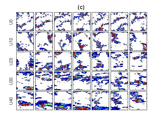
58 50

59 Figure 3.2. Snapshots of hourly surface precipitation (mm hour -1 ) for a period of 7 consecutive hours (each column), picked from the last 7 hours of the simulations. Each row corresponds to a different shear case. From top to bottom: U0, U10, U20, U30, and U40. (a) for low (b) moderate, and (c) high surface fluxes. In the case of moderate surface fluxes (Figure 3.2.b) the unsheared flow s convection is random and distributed uniformly across the domain, but less so than in the case of low surface fluxes, as there are arcs and semi-circular patterns. Under weak shear (case U10) there are organized convective clusters in part of the domain. As the shear increases further, lines of intense precipitation (in brown shading) are trailed by lighter rain (blue shading) which propagate downshear (eastward). The organization in all cases is three-dimensional. For high surface fluxes (Figure 3.2.c), convection is organized in linear forms in the absence of vertical wind shear, loses linear structure with moderate shear (U10), and transform into aggregated states in which intense precipitation only occurs in a small part of the domain. Moncrieff and Liu (2006) simulated three-dimensional propagating shear-perpendicular MCS in unidirectional quasi-constant vertical shear. Mesoscale downdrafts/density currents were important, and synoptic waves played a part in the intermittent occurrence of the MCS episodes. The small domain setup under WTG approximation in this study and lack of synoptic-scale variability likely suppress intermittency and may explain the lack of shear-perpendicular systems as prevalent convective regime in our simulations. Shear-parallel bands were observed in the eastern tropical Atlantic during GARP Tropical Atlantic Experiment (GATE), and were reproduced in simulations of that 51

60 experiment by Dudhia and Moncrieff (1987). Although there are a number of differences between those simulations and ours, there are a number of similarities between their results and those found here, including downgradient convective momentum transport discussed later in section c.3. To further quantify the impact of the shear on precipitation, Figure 3 shows time series of the domain mean daily rain rate for the different shear strengths. Statistical equilibrium is reached in the first few days. The magnitude of the temporal variability is minimized in the unsheared case, and increases with increasing surface fluxes, while it is maximized in the cases U30 and U40 for low surface fluxes (Figure 3.3.a), and in U20 for higher surface fluxes (Figure 3.3.b and c). In many of the simulations the variability is quasiperiodic, with periods on the order of days. We are interested here primarily in the timeaveraged statistics and have not analyzed these oscillations in any detail. 52

61 Figure 3.3. Time series of daily precipitation. (a) low, (b) moderate, and (c) high surface fluxes. Colors indicate the value of the shear (m s -1 ). To define a quantitative measure of convective organization, we first define a blob as a contiguous region of reflectivity greater than 15 dbz in the vertical layer 0-2 km (Holder et al. 2008). Figure 3.4.a shows a normalized probability density function (PDF) of the total (as the sum of all times for which we have data) number density of blobs, and Figure 3.4.b shows the normalized PDF of the total area of blobs in the domain for the 53

62 Figure 3.4. Normalized probability density functions (PDFs) of (a) the total number density of blobs (number every 4x10 4 km 2 ), and (b) the size of blobs in the domain (km 2 ). moderate surface fluxes case. The number of blobs decreases as convection clusters into aggregated structures with stronger shear. The areal coverage of convection increases with stronger shear as the tail of the PDF spreads towards larger areas. The other cases of surface fluxes are qualitatively similar and not shown. 54

63 b. Mean Precipitation, Thermodynamic Budget and Large-Scale Circulation 1) Mean Precipitation A key question we wish to address is the dependence of the mean precipitation in statistical equilibrium as a function of the shear. Figure 3.5 shows the domain and time mean precipitation as a function of shear for three cases of surface fluxes, as a direct model output (in red) and as diagnosed from the energy budget (in blue) as we will discuss in section c.4. The most striking feature is that for low and moderate surface fluxes, the mean precipitation is a non-monotonic function of the shear (Figure 3.5.a and b). For low surface fluxes, small shear brings the precipitation below that in the unsheared case, achieving its minimum at U20. For strong shear (U30 and U40), however, precipitation increases not only relative to the unsheared case but also above the surface fluxes, which indicates moisture import by the large-scale circulation. For moderate surface fluxes, the structure of the non-monotonicity differs from that in the low surface fluxes case. The minimum precipitation now shifts to U10, above which the behavior is monotonic. Again, strong shear is required to bring precipitation above that in the unsheared case. For high surface fluxes, the behavior is monotonic, and small shear suffices to bring precipitation above that in the unsheared case. The difference between the minimum and maximum precipitation in the high surface flux case exceeds that in the lower surface flux cases, which is also (as one would expect) manifested in parameterized large scale vertical velocity W WTG as we will show in Figures 2.8.c and f. There is no obvious relationship, however, between mean precipitation and organization. While small 55

64 Figure 3.5. Time and domain mean model output precipitation (red), derived precipitation (blue), and surface fluxes (black) as a function of the shear. (a) low, (b) moderate, and (c) high surface fluxes. shear can organize convection from a completely random state, the mean of that more organized convection need not be larger than that in the unsheared random state (Figures 2.2.a and b). 56

65 To examine the role of the cold pool on the relationship between mean precipitation and shear, we have also performed a set of similar simulations but with cold pools suppressed by setting evaporation of precipitation to zero at levels below 1000 m. Although, as expected, mean precipitation increases in these simulations relative to those in which precipitation can evaporate at all altitudes, the dependence of mean precipitation on the shear remains the same (not shown). This suggests that the cold pools are unlikely to be a key factor controlling the mean precipitation-shear relationship. 2) Moist Static Energy (MSE) budgets The moist static energy (MSE) budget can be a useful diagnostic for precipitating convection as MSE is approximately conserved in adiabatic processes. It is the sum of thermal, potential and latent heat terms. To define the basic state from which perturbations will be computed, the equilibrium vertical profiles of temperature, water vapor mixing ratio, and MSE for the unsheared case of moderate surface fluxes of 206W m -2 are shown in Figure 3.6 (other unsheared cases for low and high surface fluxes are very similar). Due to the fixed radiative cooling, the tropopause is at ~14 km, and the melting level is at ~4 km. 57

66 Figure 3.6. Vertical profiles of (from top to bottom): temperature, water vapor mixing ratio, and moist static energy (MSE) for the unsheared case of moderate surface fluxes. 58

67 Figure 3.7. Temperature, water vapor mixing ratio, and moist static energy, all expressed as differences from the unsheared case. Top row, low, middle row, moderate, and bottom row: high surface fluxes. Figure 3.7 shows the time and domain mean profiles of temperature, water vapor mixing ratio, and moist static energy, all expressed as perturbations from the same 59

68 quantities in the unsheared experiment. There is a weak sensitivity to the shear in the temperature profile for low surface fluxes, becoming larger as surface fluxes increase. Recall that the temperature is continually being strongly relaxed back towards the target profile. The temperature perturbation is positive in the mid to upper troposphere and negative in the boundary layer in the strong shear case. The moisture profile is more sensitive to the shear than temperature is, but varies little with increasing surface fluxes. Above the boundary layer the strong shear case is moister than the unsheared case by about 0.2 g kg -1 and drier in the boundary layer by about 0.5 g kg -1. The weak shear case is drier than the unsheared case at all levels for all three cases of surface fluxes. This increasing dryness with shear is also apparent in the snapshots of surface rainfall (Figure 3.2). The moist static energy variations with shear are dominated by the moisture term, are very similar for all three cases of surface fluxes, and depend non-monotonically on the shear. The non-monotonicity remains the same for all cases of surface fluxes, unlike the large-scale vertical velocity and mean precipitation. 3) Large-Scale Circulation Figure 3.8 shows the vertical profiles of large-scale vertical velocity W WTG W!"# (a)-(c), and its maximum value with respect to the vertical (d)-(f) for the three cases of surface fluxes. For low surface flux, W WTG is very weak (less than 1 cm s -1 ), and its absolute value varies little with shear. As the surface fluxes increase, W WTG increases, but the effect of the shear is much more significant in the highest surface fluxes case, where W WTG increases by 4 cm s -1 from the unsheared case to the case with the strongest shear. 60

69 Figure 3.8. (a)-(c) vertical profile of the large-scale vertical velocityw!"#. (d)-(f) W!"# W WTG Maximum. (a) and (d) low, (b) and (e) moderate, and (c) and (f) high surface fluxes. 4) Normalized Gross Moist Stability In order to diagnose the mean precipitation from the point of view of the moist static energy budget, we use the diagnostic equation for precipitation as in, e.g., Sobel (2007) or Wang and Sobel (2011); see also Raymond et al. 2009: 61

70 1 P= ( E+ H+< QR > ) < QR > H (3.2) M! Where. =! dp/g is the mass weighted vertical integral from the bottom to the top!! of the domain. P, E, H, and Q! Q R are precipitation, latent heat flux, sensible heat flux, and radiative cooling rate. We have also utilized the large-scale vertical velocity and the moist static energy introduced in the above two subsections to define M = < W WTG h z > < W WTG s > as the normalized gross moist stability, which represents z the export of moist static energy by the large-scale circulation per unit of dry static energy export. Here s is the dry static energy (sum of the thermal and potential energy only, without the latent heat term), and the overbar is the domain mean. The above equation is not predictive because we use the model output to compute the terms; in particular, we do not have a theory for M. Nonetheless, it gives a quantitative, if diagnostic, understanding of the role played by large-scale dynamics in controlling precipitation. We must first verify that our moist static energy budget closes well enough that the precipitation calculated from equation (2.6) agrees well with the model output precipitation. This is the case, as shown in blue in Figure 3.5. As shown in Figure 3.5, the variations of M with respect to shear (themselves shown in Figure 3.9) explain those in the mean precipitation. Since both surface fluxes and radiative cooling are constant in each plot in Figure 3.5, variations in M are the only factor controlling the variations in precipitation computed by equation (6), which is quite close to the actual simulated precipitation. 62

71 Figure 3.9. Normalized gross moist stability M as a function of the shear. (a) low, (b) moderate, and (c) high surface fluxes. 63

72 Maximum M means maximum export of moist static energy by the large-scale circulation per unit of dry static energy export. Since radiative cooling and surface fluxes are prescribed, the moist static energy export is also prescribed, and variations in M must correspond to variations in dry static energy export. Since dry static energy export changes can only be balanced by changes in the rate of condensation (radiative cooling, again, being fixed) and, hence, in the precipitation rate. For the case of low surface fluxes, M exceeds 1 for the cases U10 and U20; this is because of the low level subsidence and upper level ascent in the W WTG profile, with midlevel inflow bringing in relatively low moist static energy air. c. Convective Cloud Properties 1) Cloud Fraction The vertical profile of cloud fraction for the three values of surface fluxes is shown in Figure The cloud is defined as the set of grid points where the mixing ratio of cloud hydrometeors (water and ice) is greater than g kg -1. Generally, there are three peaks: a shallow peak at 1km, a midlevel peak related to detrainment at the melting level at about 4 km, and a peak associated with deep convection at 9-12 km. When the cloud fraction in the deep convective peak becomes large, we interpret it as stratiform cloud. In all three cases, the shear has almost no effect on the shallow convection. For low surface fluxes (Figure 3.10.a) the effect of strong shear is seen mainly in the midlevels, where cloud fraction increases from 30% in the unsheared flow to 60%. A 64

73 modest stratiform layer forms as cloudiness increases from 10% to 30%. Figure Cloud fraction. (a) low, (b) moderate, and (c) high surface fluxes. 65

74 For moderate surface fluxes (Figure 3.10.b) the strong shear, while causing an increase of more than 40% in the midlevel peak over the unsheared case, also leads to 100% cloud cover in the layer 9-12 km. It is also interesting to notice a transition from a single peak in the high clouds at 9 km in the unsheared and weak shear cases to a cloudy layer 5-12 km deep in the strong shear. In Figure 3.10.c near-total deep cloudiness is determined by the strong, persistent convection associated with the high surface fluxes. The shear has no effect on the cloud fraction at upper levels, since it is 100% even with no shear. The effect of shear on mid-level cloudiness is clear, however, as cloud fraction increases over 35% from the unsheared to the strongest shear flow. The cloud cover in the midlevel increases monotonically with shear, but the deep cloudiness does not (Figure 3.10.a and b), behaving instead more like mean precipitation. We discuss this further in section 3.c.3. 2) Convective Mass Flux Figure 3.11 shows the convective mass fluxes in both updrafts and downdrafts. Updrafts are defined here as including all grid points with liquid water and ice content greater than g kg -1 and vertical velocity greater than 1 m s -1, normalized by the total number of grid points. The downdrafts are defined including all grid points with vertical velocity less than -1 m s -1. The updraft mass fluxes are about twice as large as the downdraft mass fluxes. Both have two peaks, in the lower and upper troposphere, both of which strengthen by about a factor of 3 from lowest to highest surface fluxes. Despite different convective organization for different shear profiles, the vertical profiles of the updrafts and downdrafts have similar shapes. For the downdrafts, the 66

75 Figure Convective mass flux of updrafts and downdrafts. (a) low, (b) moderate, (c) high surface fluxes. 67

76 lower tropospheric peak exceeds the upper tropospheric one for all three cases of surface fluxes, and are similar for different shear strengths. The largest difference occurs in the case of highest surface fluxes, in which the downdraft in the lower peak for the smallest shear is stronger than for the strongest shear by about 20%. The effect of the shear on the upper tropospheric peak, however, is more prominent. The strongest shear causes the downdraft mass flux to strengthen by 50%. The updraft mass fluxes in the low surface fluxes case are greater in the lower troposphere than in the upper troposphere, due to the dominant role of the shallow convection, while in the moderate surface fluxes case both peaks are almost comparable, and in the high surface fluxes case the upper peak is larger due to deep clouds. Although with high surface fluxes there is an increase of 25% in the upper tropospheric updraft from the weakest to strongest shear, the effect of the shear on the updraft is smaller than in the downdraft and has negligible impact on the lower tropospheric peak, and, unlike the downdraft, is non-monotonic, similarly to cloud fraction. 3) Momentum Fluxes Another collective effect of the cloud population and its organization on the largescale flow results from vertical fluxes of horizontal momentum, including both convective momentum transport and gravity wave momentum transport (Lane and Moncrieff 2010, Shaw and Lane 2013). We evaluate these momentum fluxes as a function of the shear strength. Figure 3.12 shows the vertical profiles of the time and domain mean zonal momentum fluxes ρu'w' where u and w are the zonal and vertical 68

77 Figure Momentum fluxes. (a) low, (b) moderate, and (c) high surface fluxes. 69

78 velocity perturbations from the horizontal average, respectively, and the overbar is the horizontal mean. The magnitude of the net momentum flux is a monotonic function of the shear. It is negligible for all unsheared cases, as expected, and negative (directed down the gradient of the mean zonal wind) and peaks close to the top of the shear layer for the sheared cases. This negative momentum flux would act (if it were not strongly opposed by the imposed relaxation) to accelerate the mean horizontal wind in the lower troposphere and decelerate it in the upper troposphere and the stratosphere. The amplitude of the momentum transport also increases with surface fluxes. Interestingly, for the highest surface fluxes the momentum flux in the U10 case (Figure 3.12.c), is up gradient in the lower troposphere and peaks at about 4 km, while it is down gradient in the upper troposphere. In the 2-D analytic steering-level model of Moncrieff (1981) the updrafts tilt downshear and precipitation falls into the updrafts weakens the cold pool and causing upgradient momentum transport. With the exception of the lower troposphere in the U10 case for the largest surface fluxes, our momentum fluxes are primarily downgradient throughout the troposphere. This may be due to the fact that none of our simulations show truly long-lived, quasi-2d shear-perpendicular squall lines as in Moncrieff s model, as discussed further below. 70

79 3.4. Response to Different Shear Depths In this section we investigate the effect of varying the depth of the shear layer. We repeat the above calculations but with shear depths of 1500 m, 3000 m, 4500 m, 6000 m, and 9000 m. In each case, the wind speed is held fixed at 20 m s -1 at the top of the layer (Figure 3.1.b). Surface latent and sensible heat fluxes are held fixed at the intermediate values from the previous section, totaling 206W m -2. As of convective organization, Figure 3.13 shows snapshots of hourly surface precipitation for a period of 7 consecutive hours, chosen from the last 7 hours of each simulation. Each row corresponds to a different shear case: 1500, 3000, 4500, 6000, and 9000 m, from top to bottom. Most of these snapshots are a mixture of linear squall lines and supercell-like 3D entities, which have strong rotational components and tend to split into left and right movers (e.g., the 4500 m case in the 3 rd row of Figure 3.13). For shallow shear of depth 1500 m, convection is to some extent organized in lines normal to the shear (as seen in some of the snapshots) Nonetheless, the shear-perpendicular squall lines prevalent in analytical models (e.g., Moncrieff 1992) and 2D numerical simulations (e.g., Liu and Moncrieff 2000) do not become fully established even in the shallow shear case. Mid-level shear ( m) is associated with quasi-linear structure parallel to the shear with intense precipitating cores trailed by lighter precipitation. As the shear depth increases above that approaching the deep shear cases analyzed in the preceding sections - the quasi-linear regime is still less prominent. For deeper shear of 9000 m, convection aggregates in clusters 71

80 Figure As Figure 3 but for different shear depths. From top to bottom: 1500, 3000, 4500, 6000, and 9000 m. Figure 3.14 shows time and domain mean precipitation as a function of the shear depth. The shallowest shear layer, with depth 1500 m, produces the least precipitation, about 30% less than the unsheared case, despite a greater degree of convective organization compared to the unsheared flow (not shown). Doubling the shear layer depth almost doubles the precipitation. The mid-depth shear layers, with tops at m produce the greatest precipitation; in this sense, these intermediate shear layer depths are optimal. Although the convection is in statistical equilibrium, this is in agreement with studies of transient storms of Weisman and Rotunno (2004). While it was not the case 72

81 Figure Time and domain mean model output precipitation (red), derived precipitation (blue), and surface fluxes (black) as a function of the shear layer depth. that the optimal state produces the greatest surface precipitation in their original papers and later work, Bryan et al. (2006) demonstrated that optimal state is indeed associated with the greatest precipitation in several mesoscale models. Bryan et al. (2006) further attributed this discrepancy to numerical artifacts in the model used by Weisman and Rotunno. (2004). Increasing the shear depth above 4500 m reduces the precipitation again, with the values for 6000 m and 9000 m depths being smaller than those for the intermediate depths. We have performed simulations analogous to those in Figure 3.14 but with low and high 73

82 Figure Vertical profile of the large-scale vertical velocityw!"# for different shear depths. surface fluxes (not shown). In these simulations, we find a similar dependence of the mean precipitation on the shear depths. The relationship shown in Figure 3.14 between mean precipitation and shear depths appears to be qualitatively independent of the magnitude of the mean precipitation, at least in the regime studied here. The vertical profiles of the large-scale vertical velocity as a function of the shear layer depth are shown in Figure As we expect, the amplitude differences are largely consistent with those in the mean precipitation. The peak value, for instance, is smallest for the shallow shear case, and largest for the mid-level shear. The cases of 3000 m and 4500 m are almost identical, while there is a small increase in precipitation for 4500 m 74

83 Figure Temperature, water vapor mixing ratio, and moist static energy, all expressed as differences from the unsheared case, for different shear layer depths. 75

84 Figure Convective mass fluxes of updrafts and downdrafts for different shear layer depths. over that at 3000 m. This is due to the more abundant moisture in the lower to mid troposphere for the case of 4500 m, as shown in Figure Dominated by moisture, moist static energy has a maximum for the 4500 m case. Figure 3.17 shows the mass fluxes in updrafts and downdrafts for the different shear depths. Although the maximum mean precipitation occurs for the shear depth of 4500 m, the maximum updraft mass flux occurs at 3000 m shear depth. This demonstrates that convective mass flux need not vary in the same way as the precipitation rate. The response of the downdrafts is much weaker than that of the updrafts. In fact, the 76

85 downdraft mass flux for the shallow shear is almost identical to that for the deeper shear Figure Momentum fluxes for different shear layer depths. layers with depths 6000 m and 9000 m. Finally, Figure 3.18 shows the domain averaged time mean zonal momentum fluxes ρ uw ' ' for different shear depths. Similar to the analytic model of Moncrieff (1992), momentum flux here is down the mean gradient for all shear depths, as in Figure 3.12, and achieves the minimum at the top of the shear layer in each profile. This is likely due to momentum mixing, consistent with shear-parallel lines (Dudhia and Moncrieff 1987). The downward momentum transport is greatest when the shear is shallow: 1500 m and 77

86 3000 m deep, and becomes smaller for deep shear (9000 m); similar to the cases with uniform shear depth (Figure 3.12). This momentum flux dependence on the shear depth differs from the variations in the mean precipitation. As with other measures of organization, momentum flux apparently does not have a direct relationship to precipitation in our simulations Summary and Discussion We have quantified the effect of vertical wind shear on atmospheric convection in a series of 3-D CRM simulations with large-scale dynamics parameterized according to the weak temperature gradient approximation. We varied the shear while holding surface heat fluxes fixed. We repeated the calculations for three different values of surface fluxes. As surface fluxes are increased, the strength of the simulated convection increases, as measured by domain-averaged precipitation. Precipitation increases more rapidly than the surface latent heat flux, because of parameterized large-scale moisture convergence. The three cases thus correspond to weak, moderate and strong convection. The response of mean precipitation to shear in statistical equilibrium for the lower two surface flux cases is non-monotonic in the magnitude of the shear, with a minimum precipitation at an intermediate shear value. The shear value at which the minimum precipitation occurs is somewhat different for low and moderate surface fluxes. Only for strong shear does the precipitation exceed that in the unsheared flow. In the case of the highest surface fluxes used, the response to shear is monotonic and a small amount of shear is enough to cause the precipitation to exceed that of the unsheared flow. 78

87 The dependences of large-scale vertical velocity and the moist static energy on shear are both similar to the dependence of precipitation on shear. The dependence on shear of the normalized gross moist stability, which combines these two quantities in a way relevant to the column-integrated moist static energy budget, is found to explain the variations in mean precipitation with shear well. Despite the relative smallness of the changes in the mean precipitation with shear, shear has a strong effect on convective organization. Weak shear is sufficient to organize convection even under weak surface fluxes when the large-scale vertical motion is negligible. Stronger shear can organize convection into convective clusters and squall line-like structures with lines of intense precipitation trailed by lighter rain. As the surface fluxes and domain-averaged precipitation increase, however, convection is found to be organized even in the absence of vertical wind shear. The wind shear also has a significant effect on cloud cover, which increases with the shear (especially high clouds); convective mass flux (in particular the downdraft mass flux); and momentum fluxes, as more momentum is transported downward when the shear increases. When the total change in velocity over the shear layer is fixed but the layer depth is varied, mid-level shear depths are found to be optimal for producing maximum mean precipitation, maximum large-scale vertical velocity and maximum column moist static energy. Convective organization, for this shear depth, is very similar to that for deeper shear layers, but with more intense lines of precipitation. Confining the shear in a shallow layer dries out the atmospheric column, leaving precipitation at a minimum. 79

88 We have neglected the complications of cloud-radiation feedback by fixing the radiative cooling rate in a simple relaxation scheme. In reality, longwave radiative cooling can be suppressed by the abundant upper tropospheric ice cloud in the deep tropics, which by itself is controlled by the shear. This effect will be investigated in a separate, future study. 80

89 Chapter 4 Response of Atmospheric Convection to Vertical Wind Shear: Cloud Resolving Simulations with Parameterized Large-Scale Circulation. Part II: Effect of Interactive Radiation and Coupling with a Slab Ocean. This Chapter has two sections. In the first, I shed light on how interactive radiation plays a critical role on propagating intraseasonal disturbances in the tropics, MJO specifically, through increases in the normalized gross moist stability. Furthermore, interactive radiation modulates convective heating itself, indicating a strong coupling between the two. The second section deals with instability behavior generated by coupling slab ocean mixed layer and imposing vertical wind shear Introduction Radiative feedbacks have been shown to be an important contributor to the dynamics of tropical disturbances a range of time scales, including tropical cyclogenesis 81

90 (e.g. Bu et al 2014; Hakim et al. 2013) and intraseasonal variability (e.g., Raymond 2001; Bony and Emanuel 2005; Sobel and Maloney 2013), and in observations (e.g. Lin and Mapes 2004; Sobel et al. 2014) as well as idealized numerical modeling studies (e.g., Raymond 2001; Grabowski and Moncrieff 2002; Bony and Emanuel 2005; Wing and Emanuel 2014). By absorbing longwave radiation and re-emitting it to space at lower temperatures, clouds and water vapor warm the troposphere. Locally, regions of deep convection experience a strong reduction in the net radiative cooling compared to adjacent clear-sky regions. At the top of the atmosphere, this longwave warming is often largely (though imperfectly; Lin and Mapes 2004), offset by shortwave anomalies due to the enhanced albedo of deep clouds (e.g, Hartmann et al. 2001), so that the effect of high tropical clouds on the long-term climate is modest. However, the longwave effect is felt immediately in the atmosphere. The compensating shortwave effect is felt largely at the surface; if the surface is ocean, the heat capacity of the ocean mixed layer can delay that response enough that on short time scales, the positive feedback in the atmosphere dominates. By acting as a source of column-integrated moist static energy where that quantity already has a positive anomaly, this longwave radiative feedback can organize tropical convection (Raymond 2000; Sobel and Gildor 2003; Grabowski and Moncrieff 2004; Bretherton et al. 2005; Wing et al. 2014; Emanuel et al. 2014; Tobin et al. 2013). We expect the effectiveness of cloud-radiative feedbacks to be related to the horizontal extent, vertical structure and microphysical properties of the cloud field. These cloud properties, in turn, are influenced by a number of environmental factors. Vertical wind shear is an important such factor, in that we expect it to play a significant role in the 82

91 organization of convective cloud systems on the mesoscale. In this study, we describe studies designed to isolate the influence of vertical shear on the cloud-radiative feedback over oceans in the tropics. In the first part of this study (Anber et al hereafter AWS14), we performed CRM simulations in which we prescribed both surface fluxes and column radiative heating, and introduced a background vertical wind shear of different strengths as a control parameter. We found that under otherwise identical large-scale conditions, the precipitation can change significantly as a result of the wind shear influence, as the shear organizes the convective systems into squall line-like structures. These structures influence the convective heating and large-scale vertical motion profiles, with the relationship between heating and large-scale vertical motion parameterized by the weak temperature gradient (WTG) approximation. The different vertical motion profiles lead to different mean precipitation rates for the same export of moist static energy (with that export fixed by the imposed surface fluxes and radiative cooling), a relationship quantified by the normalized gross moist stability. In this sequel paper we perform similar model integrations, again studying the influence of vertical wind shear on tropical convection, but now with interactive radiative heating. The results are then compared to those obtained from otherwise identical experiments in which the radiative heating is prescribed to have the same profile as in the interactive radiation simulations. Our simulation design is such that we are not studying the most direct aspects of the radiative feedback on convective organization, in which the radiative heating itself 83

92 changes, since we are comparing interactive- and fixed-radiation simulations in which the radiative heating itself is the same, in the horizontal and time mean. The direct radiative feedback can be estimated straightforwardly from observations or global model simulations, as the column-integrated radiative heating anomaly per unit anomaly in column water vapor, precipitation, or other metric of convective activity (e.g., Bretherton and Sobel 2002; Su et al. 2002; Lin and Mapes 2004; Kim et al. ). Rather, we investigate the more indirect effects which result not from the change in the areally averaged radiative heating, but from the effects that interactive radiation may have on cloud structure and dynamics. These then influence the export of moist static energy via changes in the large-scale vertical motion profile. We find that these effects can be quite significant, and we are not aware of any previous documentation of them. To facilitate this study of the vertical shear influence on cloud-radiative interaction, we prescribe surface turbulent heat fluxes. This eliminates surface flux feedbacks which would occur if the lower boundary were taken to be at fixed sea surface temperature (SST). With varying vertical shear, changes in momentum transport to the surface can change surface winds from one simulation to the next, inducing strong surface turbulent flux feedbacks under fixed SST. These feedbacks are not of interest here, so we eliminate them by fixing surface turbulent heat fluxes directly. We have also conducted simulations with a slab ocean model; these increase the size of the parameter space and the range of model behavior enough that we will report on them in a separate study. We also introduce a more complex setting by coupling a mixed layer slab ocean of varying depths to the atmospheric model. In this case, more degrees of freedom are 84

93 allowed by the fully interactive SST and radiation that operate together in sheared and unsheared environments. Our main goal is to investigate the effect of interactive radiation on precipitation. After describing the modeling experiments in section 4.2, we present results from experiments with fixed surface fluxes in section 4.3. In section 4.4, we present results from experiments with an ocean mixed layer. We summarize in section Model and Experimental Design The model used here is the Weather Research and Forecast (WRF) model version 3.3, in three spatial dimensions with the same schemes used in AWS14. For experimental design and implementation of the Weak Temperature Gradient (WTG) approximation (Sobel and Bretherton 2000 and Raymond and Zeng 2005) the reader is referred to the first part of this study (AWS14). All experiments are integrated more than 40 days to achieve statistical equilibrium, and analysis of the output is conducted on the last 20 days, during which the simulations have reached statistical equilibrium. To obtain the reference temperature profile required for WTG, we follow a standard procedure (e.g., Sobel and Bretherton 2000; Raymond and Zeng 2005; Wang and Sobel 2011; Daleu et al. 2015). We first perform a radiative-convective equilibrium (RCE) experiment at a fixed SST of 28 with interactive radiation, reaching equilibrium at about 60 days. Results from this experiment are averaged over the last 10 days after equilibrium to obtain statistically equilibrated temperature and moisture profiles. Figure 1 shows the resulting vertical profiles of (a) potential temperature and (b) moisture. These 85

94 profiles are then used to initialize runs with parameterized large scale circulation, and the temperature profile is used as the target profile against which perturbations are computed in the WTG runs. For numerical experiments with interactive radiation, the NCAR Community Atmosphere Model (CAM 3.0) shortwave and longwave radiation schemes Collins et al. (2004) are adopted. Diurnal and seasonal cycles are removed and the top of the atmosphere incident solar flux is set to 400 W m 2. For WTG runs without vertical wind shear, we prescribe total turbulent surface fluxes of heat and moisture at three different values: low (140 Wm!! ), moderate (180 Wm!! ), and high (220 Wm!! ); these variations are achieved holding the sensible heat flux fixed at 20 Wm!!, while the latent heat flux takes on values of 120, 160, and 200 Wm!!. We constrain the vertical wind shear by relaxing the horizontal mean zonal wind towards a prescribed profile with a time scale of one hour, as AWS14. We vary the shear depth over three layers; shallow (1500 m), midlevel (4500 m), and deep (12000 m), while holding the target wind speed at the top of the shear layer constant at 20 m/s, while keeping it zero at the surface (see Fig.1 of AWS14). Surface fluxes for this set of experiments are held fixed at 180 Wm!!. Clouds and water vapor then evolve freely and strongly influence the radiative heating profile. The time-and domain-averaged radiative heating profiles for this set of experiments is shown in Figure 4.1.a for the unsheared environment with different surface fluxes, and Figure 4.1.b for different shear depths with intermediate surface 86

95 fluxes. For either low surface fluxes or shallow shear there is a cooling throughout the whole atmospheric column that reaches 1 K/day in the upper troposphere. For higher surface fluxes or deeper shear, there is a significant radiative heating in the mid-to upper troposphere, exceeding 5 K/day for high surface fluxes. Above 10 Km there is a sharp drop in the radiative heating profile due to the strong emission of longwave radiation from cloud top, with radiative cooling exceeding 10 K/day for strong surface fluxes or deep shear. To compare the effect of interactive radiation on the cumulus ensemble interacting with the parameterized large scale dynamics, we perform identical experiments for both sheared and unsheared runs except that now we prescribe the radiative cooling profile in Figure 4.1 and keep it fixed and non-interactive with clouds or water vapor at every time step. This way we keep the same time-and domain- averaged radiative cooling in both interactive and non-interactive radiation experiments. As surface fluxes are already fixed, this means both the equilibrated time mean column-integrated moist static surface fluxes and net radiative cooling are identical in pairs of interactiveand fixed-radiation experiments. Any differences in the time mean column moist static energy budgets must be due to the export term, which is controlled by the large-scale vertical velocity profile. For the second part of this study, the reference temperature profile is taken from an RCE experiment with fully interactive SST (and radiation) by coupling a simple slab ocean mixed layer. The mixed layer temperature is predicted using the equation of energy budget: 87

96 dt ρ HC = LH SH + LW + SW dt Z (km) (a) 140 W/m W/m W/m Z (km) (b) 1500 m 4500 m m K/day Figure 4.1. Domain averaged radiative cooling profile as a function of (a) surface fluxes, and (b) shear depths. 88

97 where T is sea surface temperature, ρ, water density (1000 Kg/m 3 ), C, heat capacity of water (4180 J. kg!!. K!! ), H, depth of the mixed layer (1 meter), LH, surface latent heat Precip (mm/day) Precip (mm/day) interactive prescribed bud. interactive bud. prescribed (a) sfc fluxes (W/m 2 ) (b) Shear depth (m) Figure 4.2. Domain averaged surface precipitation as a function of (a) surface fluxes, and (b) vertical wind shear depths, for simulations of interactive (blue), and prescribed (red) radiation, stars denote precipitation from model output, and squares denote precipitation diagnosed from the moist and dry static energy budgets. 89

98 flux, SH, surface sensible heat flux, LW, net longwave radiative flux (positive downward, W/m 2 ), SW, net shortwave radiative flux (positive downward, W/m 2 ). Equilibrium is achieved after approximately 7 years of integration. The long integration is necessary because of strong coupling between the atmosphere and underlying ocean and the heat capacity of the slab ocean (Cronin and Emanuel 2013). In the equilibrium, mixed layer temperature is ~ K, and mean precipitation is 3.5 mm/day. Equilibrated reference temperature profile averaged for the last year for WTG runs Fixed Surface Fluxes Figure 4.2. shows time and domain averaged precipitation, P, as a function of (a) surface fluxes and (b) wind shear, for experiments with interactive radiation (blue) and prescribed radiation (red). In all experiments interactive radiation produces significantly less precipitation than prescribed radiation. The difference monotonically increases with surface fluxes (Fig.4.2.a); about 1mm/d for small surface fluxes, and reaches 3 mm/d and 5 mm/d for the moderate and high surface fluxes, respectively, while remains nearly constant with the shear (Fig.4.2.b). Mid-level shear produces the greatest precipitation in both interactive as well as prescribed radiation, in agreement with the first part of this study and others (e.g. AWS14, Weisman et al. 2004), confirming the robustness of this non-monotonic relation between shear and precipitation. Furthermore, precipitation is diagnosed from the vertically integrated budget of the moist and dry static energy as: 90

99 P = 1 M (L + H + Q R ) Q R H where L,H, < Q! >, and M are the latent heat flux, sensible heat flux, the vertically integrated radiative heating, and the normalized gross moist stability, respectively. The latter is defined as M = W h z W s z where W, s, and h are the large-scale vertical velocity, dry, and moist static energy (MSE) respectively, brackets denote mass weighted vertical integrals, and overbars are domain 15 (a) 140 W/m 2 15 (b) 180 W/m 2 15 (c) 220 W/m Z (km) Z (km) Z (km) cm/s cm/s cm/s 15 (d) 1500 m 15 (e) 4500 m 15 (f) m Z (km) Z (km) Z (km) cm/s cm/s cm/s Figure 4.3. Domain averaged large scale vertical velocity W WTG for different surface fluxes (a)-(c), and different shear depths (d)-(f), for simulation of interactive (continuous) and prescribed noninteractive (dashed) radiative profiles. 91

100 and time mean. The above equation gives a very good agreement with the model output as indicated in Fig.4.2 with squares symbols, which helps interpret changes is P. To understand the behavior of precipitation in the presence of cloud-radiation interaction, we look at the large scale vertical motion W!"#. Figure 4.3 shows the vertical profile of the large scale vertical motion for different surface fluxes ((a)-(c)) and different shear depths ((d)-(f)) for interactive (continuous) and prescribed (dashed) radiative cooling. In all cases, when radiation is interactive the large scale vertical motion exhibits similar vertical structure than when radiation is prescribed, but with a sharper peak at about 10 km and stronger subsidence in the lower levels (except the opposite of a shallow shear case Fig.4.3.d), especially for the high surface fluxes and deep shear cases. A closer look at the peak and subsidence of the large-scale vertical motion is shown in Figure 4.3 as the maximum and minimum W!"#. The peak amplitude of the vertical motion is a monotonically increasing function of the surface fluxes and the shear depth for both interactive and prescribed radiative heatings. However, there are significant differences between the two mean profiles. Cloud-radiation interaction introduces positive anomalies in the peak amplitude of vertical motion through heating anomalies by trapping longwave radiation in the high anvil clouds. Except for the shallow shear depth where the heating anomalies are negative, such heating anomalies increase with increasing surface fluxes ((a) and (c)) or shear depth and reach maximum amplitude for the highest surface fluxes and largest shear depth. 92

101 The most striking feature in the large scale vertical velocity structure, is the significant subsidence in the lower troposphere which indicates strong downdrafts resulting from evaporative cooling. For low and moderate surface fluxes, interactive radiation introduces a small increase in subsidence, and for shallow and midlevel shear the difference in subsidence is small. However, for the high surface fluxes and deep shear cases interactive radiation has a remarkable effect strengthening the subsidence. This is particularly important in the moist static energy budget and tends to reduce the mean precipitation over the prescribed profiles (Fu et al. 1993). 93

102 (a) MAX W WTG cm/s interactive prescribed (b) MIN W WTG cm/s surface fluxes (W/m 2 ) cm/s interactive prescribed (c) MAX W WTG (d) MIM W WTG 0.5 cm/s Shear depth (m) Figure 4.3. Large scale velocity of maximum (a),(c) ascending motion in the upper troposphere, and (b),(d) descending motion in the lower troposphere. (a) and (b) are cases of different surface fluxes, and (c) and (d) for different shear depths. Simulations of interactive and prescribed non-interactive radiation are in blue and red, respectively. 94

103 1.5 1 interactive prescribed (a) M sfc fluxes (W/m 2 ) (b) 1.5 M Shear depth (m) Figure 4.5. Normalized gross moist stability as a function of (a) surface fluxes, and (b) vertical wind shear depths, for simulations of interactive (blue), and prescribed, non-interactive (red) radiation, dashed line shows M=1. The results of interactive radiation on the thermodynamics can be usefully interpreted in terms of the normalized gross moist stability (e.g. Neelin and Held 1987; Sobel 2007) shown in Figure 4.5, and defined above as the export of moist static energy normalized by the export of dry static energy. Increasing surface fluxes or shear depth while holding the radiative heating prescribed, does not have a significant impact on M. 95

104 For interactive radiation, as surface fluxes and shear layer increase, M increases strongly, exceeding 1 for greatest surface fluxes and shear depth. M greater than 1 means that the export of moist static energy exceeds the export of dry static energy as seen in intraseasonal variability (e.g. Wang et al. 2015; Sobel et al. 2014). More importantly, this means any increase in radiative heating or surface fluxes for M > 1 cannot efficiently increase rain since P is inversely proportional to the product of 1/M and these MSE sources. This is expected with midlevel inflow and low-level outflow, as the W WTG profile shows (Figure 4.3.a). Thus, when moisture is transported by W WTG and vertically averaged, it results in some cancellation between the upper and lower levels. The behavior of M leads to two important points: 1) As Schematically shown in Figure 4.6 (see Fig.6 of Kim et al. 2014), a peak in convective activity associated with the onset of Madden Julian Oscillation marks a peak in vertically integrated MSE (h) anomalies over the Indian Ocean. Vertically integrated radiative heating and vertical advection of MSE (V.ADV) are in-and-out of phase with h, respectively, cancelling out each other s effect on h. On one hand, positive anomalies of vertical advection to the east of h are associated with M<1 and cause the eastward propagate (Kim et al. 2014). On the other hand, negative anomalies associated with M>1 are holding back h from propagating eastward. However, as shown in Fig.5.3, the behavior of M>1 is induced by the effect of interactive radiation. Hence, we can get to the conclusion that interactive radiation plays the role of retarding the eastward 96

105 propagation of MJO. That is, if the case of M>1 exists eastward of h (as in prescribed radiation), convective anomalies would have stayed in place not be moving eastward. Figure 4.6. Schematic showing anomalies of vertically integrated MSE h (black), radiative heating < Q R > (blue), and vertical advection of MSE V.ADV (red). Dashed line mark zero anomalies. 2) In the tropics, the dominant balance in the thermodynamic equation is between adiabatic cooling by the large scale vertical motion and diabatic heating consisting of convective and radiative heating. Therefore, the difference in the vertical profile in W WTG between interactive and non-interactive radiation results from different convective heating in both cases since time-and domain-mean radiative profiles are identical. This 97

106 shows that convective and radiative heating are tightly coupled and ignoring interactive radiation might lead to biases in convection. Z (km) (a) 140 W/m W/m W/m Z (km) (b) 1500 m 4500 m m K Figure 4.7. Domain mean profile of temperature anomalies, as departure from RCE profile, as a function of (a) surface fluxes, and (b) vertical shear depths. 98

107 As a final remark in this section, it is interesting to look at the temperature anomalies introduced by interactive radiation. Figure 4.7 shows the mean temperature anomalies from the RCE temperature profile as a function of surface fluxes (a), and shear depths (b). The low surface fluxes and shallow shear cases show heating anomalies throughout the atmosphere. However, as the surface fluxes or shear depth increase, the heating anomalies increase in the upper troposphere, while the cooling anomalies decreases in the lower troposphere. These temperature anomaly profiles indicate a more stable environment as usually observed in Mesoscale Convective Systems (Houze 1989) with large horizontal extent of stratiform anvil clouds that serve as incubating environment for tropical depressions as noted by Raymond and Sessions 2007, and Bister and Emanuel Coupling with a mixed layer Variability in sea surface temperature regulates deep convection over tropical oceans, and influence atmospheric variability on similar timescales. Also, atmospheric variability is expected to co-vary with the mixed layer temperature as observations as well as numerical studies show (e.g. Waliser 1996; Woolnough et al. 2000; Vecchi and Harrison 2002; Gildor and Sobel 2003; Sobel et al. 2008, and 2010). Therefore, the two way interaction is a key feature of the coupled dynamics. In this section we explore the response of a coupled tropical ocean atmosphere variability to vertical wind shear. We present particular cases of sheared flow in which 99

108 the solution exhibits oscillatory behavior. That is deep shear of 30 m/s speed over 12 km depth. Such strong shear has been observed during the active phase of the MJO in the Indian Ocean (e.g., Johnson and Ciesielski 2013, Sobel et al. 2014) when low level westerly reaches 15 m/s and upper level easterly exceeds 20 m/s. Results even stronger shear (or mid level shear with similar strength) exhibit similar behavior and are not shown. 10 Precip (mm/day) cm 1m 10m 50m mixed layer depth Figure 4.8. Domain averaged surface precipitation as a function of the mixed layer depth for unsheared environment. In the unsheared environment, equilibrium mean precipitation is a weak function of the mixed layer depth, as shown in Figure 4.8. Precipitation is almost constant (~6.5 mm/d) for 10 cm, 1 m, and 10 m depth, and decreases to about 3.7 mm/d for 50 m depth mixed layer showing the nonlinear dependence on the mixed layer depth. In all these experiments rain rate time series shows some enhanced randomness, but no regular oscillatory behavior is found (not shown). 100

109 For a sheared flow of 30 m/s over the depth of the troposphere, Figure 9.3 shows domain mean (a) precipitation in mm/day, (b) surface fluxes, (c) net radiation, (d) absorbed shortwave at the surface (incident minus reflected), (e) net energy flux at the surface, (f) SST, and (g) column water vapor. Precipitation has pulse-like oscillations with rainy periods approximately every 10 days, with magnitude exceeding 20 mm/day, followed by dry periods of close to zero in magnitude. Surface fluxes (Fig. 3.9.b) and precipitation (Fig. 3.9.a) are nearly in phase with each other, and rainfall maxima coincide with the maxima in surface fluxes. On the other Figure 4.9. Time series of domain averaged (a) precipitation in mm/d, (b) surface fluxes (latent + sensible), (c) net radiative cooling, (d) absorbed shortwave fluxes at the surface (incident minus reflected), (e) Net energy flux at the surface all in Wm!2, (f) SST in K, (g) column water vapor in millimeter. Case of mixed layer depth of 1 m, and shear of strength 30 m/s over the depth of 12 km. 101

110 hand, column net radiation (Fig. 3.9.d) increases at about the same time as precipitation during the onset of a rainy period, but the radiation anomaly lasts much longer even after the system transitions into a dry period. This overcast state associated with the radiation anomaly is maintained for ~5 days. Such cloudy overcast states are fundamentally different from the cloud-free dry instability of the multi-equilibria discussed in previous studies (e.g., Bretherton et al. 2005, Emanuel et al. 2014, Wing et al 2014). Inspection of the large scale vertical motion time series in Figure 4.10 shows a transition from a single to a second baroclinic mode. The later operates to maintain the dry state and indicates 15 W WTG (cm/s) Z (km) days 4 Figure Time series of the large scale vertical velocity W WTG for the case of mixed layer 1m deep, and shear of strength 30 m/s over the depth of 12 km. advection of the stratiform cloudiness ahead of the disturbance due to the strong upper level winds imposed by the vertical wind shear in this case. As discussed earlier, this thick anvil of stratiform clouds is a result of cloud-radiation interaction that produces a 102

111 second baroclinic mode in the large scale vertical velocity as seen in observations (Wang et al. 2015). Time series of the mixed layer temperature show oscillation between 296 K and 301 K. But these oscillations are highly non-sinusoidal: the warm states are very brief (~ 1day), while the cold states, corresponding to the sustained radiation anomalies in the dry states, is maintained for 3-4 days. Column water vapor (Fig. 3.9.g) varies over a relatively small range from mm. The mechanism for instability and oscillations may be that the imposed appropriate strength of the vertical wind shear induces horizontal vorticity near the surface as well as cold pool that enhance surface enthalpy fluxes. The latter lead to stronger deep convection and rainfall. Stratiform in the upper level, resulting from cloudradiation interaction, blocks the surface from receiving shortwave (Fig. 3.9.d), exhausting the supply of energy to the surface and reducing SST. Lower SST under the controlled atmospheric temperature via WTG leads to large scale descent, and suppressed convection. As the mixed layer temperature gradually recovers due to increasing shortwave at the ocean surface, eventually reaching a critical value, deep convection is activated. The Time scale of the oscillations depends on the mixed layer depth. This is shown in Figure 4.11, which is similar Fig. 3.8 but with a mixed layer depth of 10 m and imposed wind shear of speed of 15 m/s over a depth of 12 km. The period of the oscillations is approximately every 50 days, and the increase of surface fluxes and SST during the suppressed phase is gradual rather than sharp as in the 1 m mixed layer depth 103

112 case. In all cases, stronger wind shear does not affect the oscillation s frequency or the time for surface recovery. Also, instabilities in the later case occur for weaker shear than in the case of shallower mixed layer. The mixed layer temperature shows highly nonlinear oscillations. Its recovery after cooling is characterized by 2 quasi-linear stages: (1) the overcast stage, similar to that identified in the 1 meter mixed layer case, lasting ~ 10 days during which cloud and radiation anomalies are gradually dissipated, and (2) the second stage last 20 days when Figure As Fig.3.8, but for mixed layer depth of 10 m, and shear strength of 15 m/s over the depth of 12 km. 104

113 precipitation is only 1-2 mm/day, column net radiation cooling is nearly constant (~-120 W/m2), surface fluxes are sustained at 150 W/m2, and the net surface energy flux remains close to zero. The second stage is absent in the 1 meter mixed layer case. Unlike the 1 m mixed layer case, column water vapor varies over a large range in the 10 m case, from ~25 mm in the dry period to ~47 mm in the wet periods. Time scale of column water vapor recovery is more than 20 days and during the majority of the period of recovery rain is small and net radiative cooling is nearly constant. Inspection of the large scale vertical velocity profile indicates descent in the upper troposphere and no ascent in the lower troposphere. The latter feature is responsible for the build-up of water vapor in that stage. It is remarkable that instabilities here are similar to those in Gildor and Sobel 2003 and Maloney and Sobel 2004 despite that they did not consider wind shear at all, whereas here instabilities are generated spontaneously in response to the imposed strong wind shear; which resembles that associated with the MJO during the active phase. Note that the oscillatory behavior appears only if the three ingredients coexist; coupling of a mixed layer slab ocean of a large heat capacity, proper shear strength, and interactive radiation. We have done experiments in which only two of the three factors exist and no oscillatory behavior was found. We also have done experiments in which the shear relaxation timescale was altered from 1 hour to 1 day, the oscillations period was modulated from ~ 10 days (in the case of 1m mixed layer depth) to 3 days. This is because of the longer persistence of the anvil stratiform by stronger imposition of vertical shear. Finally, the thermodynamic relaxation timescale is increased to 5 days to 105

114 asymptotically approach the RCE state; the system does not exhibit oscillations. This clearly accentuates the crucial role of the coupling of large scale circulation in intraseasonal disturbances Summary In this study we have presented results of the effect of cloud-radiation interaction in an idealized framework of a 3D cloud resolving model with parameterized large scale circulation. We have experimented with this effect in different model settings including fixed surface fluxes of heat and moisture of low, moderate, and high magnitudes, with different imposed vertical wind shear strengths, and interactive SST by coupling the atmospheric model to a slab ocean mixed layer of different depths. When surface heat fluxes are prescribed, interactive radiation has a significant impact on ensembles of cumulus clouds interacting with the large scale circulation, if either high surface fluxes are large and/or the shear layer is deep, by generating an envelope of high anvil clouds that extend over a wide horizontal area. The stratiform clouds then trap longwave radiation in the mid to upper levels and cools the lower atmosphere through generation strong downdrafts. Such cloud system is manifested as a second baroclinic structure of the large scale vertical velocity in a way such that there is a large ascending motion in the mid-to upper levels and a descending motion in the lower levels (and hence evaporative cooling) resulting in a large normalized gross moist stability as seen in observational studies of intraseasonal variability (e.g. Wang et al. 2015). 106

115 It is important to stress that this structure is a result of a radiative profile interacting with clouds and water vapor, that is when the radiative profile is held fixed with the same vertical shape to that produced in simulations with interactive radiation, large scale vertical velocity mode was quite different. As a result, gross moist stability and precipitation differ greatly from those obtained with fixed radiation. Gross moist stability, now, exceeds 1, and mean surface precipitation decreases because of the enhanced evaporation of falling precipitation by strong downdrafts. When coupling a mixed layer slab ocean of varying depths, under certain conditions he system may exhibit instability behavior of wet periods followed by dry ones that last for longer times. In addition to interactive radiative profile, the conditions are vertical wind shear of certain strength and a mixed layer of appropriate depth. If any of the three conditions is absent the system attains an equilibrium, non-oscillatory solution. For example, mean precipitation in model settings with a shallow mixed layer of depth 10 cm has a equilibrium mean precipitation of about 6.5 mm/day that is almost invariant under the shear. Also, unsheared environment with deeper mixed layer does not support oscillatory solution. Our results here differ somewhat from those proposed by Sobel and Gildor 2003 and Raymond In the former wind-evaporation feedback is shown to play a significant role in enhancing surface enthalpy fluxes, while in the latter surface fluxes are enhanced through vorticity induced by the convergence from a pre-existing rain, due to instability of the environment to large-scale vertical motion due to cloud-radiation interaction. While we do not have equatorial beta-plane dynamics, the fact that we need 107

116 strong shear to active these oscillations conforms the critical roles of cloud-radiation feedback. 108

117 Chapter 5 Modeling the Diurnal Cycle in the Amazon in the context of the Weak Temperature Gradient In this chapter, I introduce a framework in the context of previous chapters where the hydrological cycle in the Amazon basin is properly modeled. The atmospheric model is coupled to Noah land surface model, and initialized with the observed state of the Amazon basin. The only input to the model (along with solar insolation) is the atmospheric sounding in the wet and dry seasons. The simulations provide a stunning matching with the observed diurnal of precipitation, surface fluxes, and radiative fluxes and help foster our understanding of the land-atmosphere interaction Introduction Tropical forests, and the Amazon in particular, are the biggest terrestrial CO 2 sinks on the planet, accounting for about 30% of the total net primary productivity in terrestrial ecosystems. Hence, the climate of the Amazon is of particular importance for the fate of global CO 2 concentration in the atmosphere (Achard et al. 2004). Besides the difficulty of estimating carbon pools (e.g. Cai et al. 2014; Hoffman et al. 2014; Achard et al. 2004), our incapacity to correctly predict CO 2 fluxes in the continental tropics largely 109

118 results from inaccurate prediction of tropical climate (Achard et al. 2004; Hoffman et al. 2014; Todd-Brown et al. 2013; Cox et al.2013). More frequent and more intense droughts in particular are expected to affect the health of the Amazon and its capacity to act as a major carbon sink (Gatti et al. 2015; Lee et al. 2013; Reichstein et al. 2013). The land surface is not isolated though but interacts with the local weather and climate through a series of land-atmosphere feedback loops, which couples the energy, carbon and water cycles through stomata regulation and boundary layer mediation (Arellano et al. 2012). Current General Circulation Models (GCMs) fail to correctly represent some of the key features of the Amazon climate. In particular, they i) underestimate the precipitation in the region (Pascale et al. 2014; Martins et al. 2014), ii) do not reproduce the seasonality of either precipitation (Pascale et al. 2014; Martins et al. 2014) or surface fluxes such as evapotranspiration (Gonçalves et al. 2013), and iii) produce errors in the diurnal cycle and intensity of precipitation with a tendency to rain too little and too early in the day (Dai 2006; Bechtold et al. 2014). In the more humid Western part of the basin, surface incoming radiation, evapotranspiration, and photosynthesis all tend to peak in the dry season (Da Rocha 2009; Fisher et al. 2009; Restrepo-Coupe et al. 2013) whereas GCMs simulate peaks of those fluxes in the wet season. Those issues might be related to the representation of convection and vegetation water stress in GCMs. We here show that we can represent the Amazonian climate using a strategy opposite to GCMs in which we resolve convection and parameterize the large-scale circulation. The simulations lack many of the biases observed in GCMs and correctly predict the variation of the surface heat fluxes and precipitation in the dry and wet season of the Amazon. Besides top of the atmosphere insolation, the simulations require the 110

119 horizontal mean temperature profile as an input. We demonstrate that this profile, whose seasonal cycle itself is a product of the coupled land-atmosphere dynamics, mediates the seasonality of the Amazonian climate by modulating the vertical structure of the largescale circulation in such a way that thermal energy is less effectively ventilated in the rainy season Methods Model configuration: We use the Weather Research and Forecast (WRF) model version 3.3, in three spatial dimensions, with doubly periodic lateral boundary conditions. The experiments are conducted with Coriolis parameter f = 0. The horizontal domain size is km 2 with a grid spacing of 2 km. There are 50 vertical levels in the domain height extending to 22 km, with 10 levels in the lowest 1 km. Gravity waves propagating vertically are absorbed in the top 5 km to prevent unphysical wave reflection off the top boundary by using the implicit damping vertical velocity scheme (Klemp et al. 2008). The 2- Dimensional Smagorinsky first order turbulent closure scheme is used to parameterize the horizontal transports by sub-grid eddies. The Yonsei University (YSU) first order closure scheme is used to parameterize non-local boundary layer turbulence and vertical subgrid-scale eddy diffusion (Hong and Pan 1996). The surface fluxes of moisture and heat are parameterized following Monin-Obukhov similarity theory. Microphysics scheme is the Purdue-Lin bulk scheme (Chen and Sun 2002) that has six species: water vapor, cloud water, cloud ice, rain, snow, and graupel. Radiative fluxes are determined 111

120 interactively using the NCAR Community Atmosphere Model (CAM 3.0) scheme for shortwave and longwave radiation. Both surface and radiative fluxes are fully interactive (Collins et al. 2004). The atmospheric model is coupled to the Noah land surface model (LSM) (EK 2003) that has four soil layer of located at 10, 30, 60, and 100 cm depth. The LSM provides four quantities to the atmospheric model: sensible heat flux, latent heat flux, upward longwave radiation, and upward shortwave radiation off the ground. The LSM prognostic land states are: surface skin temperature, volumetric total (liquid and frozen) soil moisture at each layer, soil temperature at each layer, canopy water content. All the model integrations last for 30 days. We have performed a sensitivity test on the initial conditions and they had no influence on the results. The reference, target temperature profile is time-independent in each season and does not include diurnal variations. Diurnal cycle is driven by diurnal cycle of radiation at the top of the atmosphere. Mean diurnal solar insolation in the dry season was held fixed at 415 W m -2 and in the wet season at 430 W m -2, reflecting values at Manacapuru Surface observations: We used eddy-covariance data from the K34 station located in Estação Experimental de Silvicultura Tropical 02º 37' S, 60º 09' W, located around 60km from Manaus. We have used data from 2000 to 2006 available at ORNL.gov (Saleska et al We used quality controlled eddy covariance data, based on outliers comparison, wind speed (acceptable variation is two 112

121 standard deviation units form the linear regression), and unresponsive sensor checks. Eddy covariance measurements typically cannot correctly measure in the presence of dew, thus foggy conditions are under-sampled, which should reduce the actual overall latent heat flux compared to the one observed Results: Temperature Sounding Seasonality We use the Weather Research and Forecasting (WRF) model at 2km horizontal resolution. This resolution has been shown to be sufficient to resolve convection (explicit convection) and to correctly represent the sign and magnitude of the land-atmosphere interaction feedback (Hohenegger et al. 2009) contrary to GCMs, which tend to exhibit soil moisture-precipitation feedbacks of opposite sign to that observed. We parameterize the large-scale domain average vertical motion as a function of internally resolved convection using the weak temperature gradient (WTG) approximation (Methods). The WTG approach has been used in many previous studies of tropical atmospheric dynamics to represent the feedback between locally resolved convection and larger-scale circulation (Anber et al. 2014; Wang et al. 2013; Sobel and Bretherton 2003; Sobel et al. 2001). Under WTG, we diagnose the large-scale vertical motion in the entire modeled horizontal domain as that which induces a vertical advective potential temperature tendency which relaxes the model s domain-averaged potential temperature to that of the observed mean seasonal atmospheric sounding. The same large-scale vertical motion is then also used for vertical advection of moisture. 113

122 25 dry wet (a) 25 (b) θ wet θ dry Z (km) K K Figure 5.1. (a) Monthly mean observed atmospheric potential temperature profile in the wet (February) and dry season (September) observed in 2014 at Manacapuru, near Manaus, Brazil (3 12' 46.70" S, 60 35' 53.0W) using radiosounding and used as reference profiles for the weak temperature method. (b) Atmospheric potential temperature difference between the wet and dry season. The target temperature profile of the WTG method, representative of the wetter part of the Amazon, is taken from the 2014 Atmospheric Radiation Measurement (ARM) mobile facility located at Manacapuru, near Manaus, Brazil (3 12' 46.70" S, 60 35' 53.0" W). The profiles are averaged over the month of February for the wet season, and September for the dry season, as shown in Figure 5.1.a. At the surface (where WTG is not directly applied, see methods) the dry profile is warmer by about 5K reflecting higher surface heat fluxes (Figure 5.1.b). In the mid-troposphere the wet profile is warmer by more than 114

123 Figure 5.2. Monthly mean tropical potential temperature at 7 pressure levels from near surface to lower stratosphere, averaged during the period from 1979 to 2014 using the ERA interim global reanalysis dataset. Left column, mean potential temperature at February; middle column, September; right column: difference between Februray and September. Over Amazon, wet season is generaly cooler than the dry near the surface and the tropopause, but warmer in the free troposphere, consistent with observation (Figure 5.1). 115

124 1K. In the stratosphere, the wet profile is colder by more than 5K due to seasonal migration of tropopause. All these differences are consequences of the seasonal march itself; the warmer troposphere and cooler lower stratosphere are typical differences between states of stronger and weaker deep convection (Holloway and Neelin 2007). Here the ultimate cause is presumably the stronger insolation in the wet season; it is in part itself an outcome of land-atmosphere interactions, as the tropospheric temperature difference between the two seasons in the adjacent regions has opposite sign (Figure 5.2). Since we assume this seasonal difference in temperature profiles, our simulations do not predict the seasonal changes purely as a function of external boundary conditions and forcings. Rather, we predict part of the solution including precipitation, clouds, and surface fluxes given another, the free atmospheric temperature. This allows us to understand the mediation of convection and land-atmosphere interaction by the atmospheric temperature, similar to what has been done in studies of tropical cyclones and the Madden-Julian oscillation (Raymond and Sessions 2007). 116

125 25 20 wet dry Z (km) W WTG (cm/s) Figure 5.3. WRF modeled domain-average large scale vertical verlocity for the wet and dry seasons averaged over the simulation period Diurnal Cycle and Seasonality of the Large Scale Variables In the wet season, the modeled large-scale vertical velocity is ascending throughout the whole troposphere (Figure 5.3). In the dry season, there is descending motion above the surface until about 2 km, ascent until about 5 km, another shallow layer of weak descent, and ascending motion again above about 7 km. The reduction of the vertical motion profile in response to the imposed free-tropospheric warming and lower tropospheric cooling causes the export of moist static energy by the large-scale 117

126 circulation, or the normalized gross moist stability (NGMS), to decrease significantly from the dry to the wet season. This allows precipitation to increase in the wet season relative to the dry, despite the absence of an increase in surface fluxes or radiative heating. The precipitation increase, in turn, moistens the land surface, an important factor leading to the differences in cloud between the wet and dry seasons. In the dry season, convection starts in the morning (10 local time) manifest first in a sharp increase in midlevel cloud at that time coverage (Figure 5.4.b and Figure 5.5.b), and then a more gradual transition to deep convection in the afternoon (Figure 5.4.a Figure 5.5.b). Midlevel cloud cover dissipates overnight into the early morning. The overall cloud cover is relatively small during daytime, and higher in the afternoon and evening, as observed, but opposite to what GCMs predict as mentioned above. The smaller cloud cover during daytime drives the surface fluxes, and in particular evapotranspiration and photosynthesis, by allowing more solar radiation to reach the surface (Figure 5.5). In the wet season, the diurnal cycle of cloud cover exhibits a different behavior. Above the surface, a distinct layer of fog is maintained by surface radiative cooling and 118

127 1 (a) High Cloud Cover 0.5 fraction (100%) (b) Mid Cloud Cover (c) Low Cloud Cover/Mist wet dry Hours Figure 5.4. Diurnal cycle of fractional cloud cover for (a) high (9-16 km), mid-level (3-5 km), and (c) mist ( m) clouds in the WRF simulations. 119

128 Figure 5.5. Composite of the WRF simulated 2-Day cycle of fractional cloud cover for (a) the wet and (b) dry season. 120

129 and reduces net surface shortwave radiation and evapotranspiration (Figure 5.6.b). The latent heat flux (Figure 5.6.a) and surface temperature (not shown) are less in the wet Latent heat flux (W m -2 ) obs. wet WRF wet 800 a) obs. dry b) WRF dry 700 Net shortwave at surface (W m -2 ) Hours Hours Figure 5.6. Diurnal cycle of (a) latent heat flux, and (b) net shortwave at the surface, for WRF modeled (thick) and climatology of observed (thin) fluxes. Shading reflects standard deviation of the observed flux throughout the month. Observed fluxes are taken from the climatology of eddycovariance fluxes observed at K34 station in the Reserva Biológica do Cuieiras. We note that surface observations have difficulty observing in the presence of dew (eddy-covariance measurements typical cannot correctly record measurements) so that the observations typically omit foggy situation, with an overrepresentation of relative clear days compared to foggy days. season than in the dry season, because of the lower surface shortwave radiation induced by the fog layer, which compensates for the higher water availability in the soil and 121

130 related lower Bowen ratio (from diurnal averaged of 0.4 in the dry season to 0.32 in the wet season based on eddy-covariance data). We note that surface observations have difficulty observing in the presence of dew (eddy-covariance measurements cannot correctly record measurements) so that most foggy days are not captured by surface 100 dry wet (b) Cloud Radiative Forcing 50 0 W/m SWCRF NETCRF LWCRF Figure 5.7. (a - left) Diurnal cycle of modeled (think line) and observed (thin line) precipitation from CPC MORPH along with standard deviation of the observations (shaded area). (b - right) Cloud shortwave (SWCRF), longwave (LWCRF), and net (NETCRF) radiative feedback for the wet and dry seasons as simualted by WRF with the weak temperature gradient method. observations so that clear days with higher latent heat flux are overrepresented in the observations In agreement with observations (here CPC Morphing Technique (CMORPH) (Joyce et al. 2004) data averaged over 10 years ( ) for the month of February and September for the wet and dry seasons, respectively), our simulated precipitation 122

131 maxima occur in the early to late afternoon in both seasons, with greater amplitude in the wet season (Figure 5.7.a). Convective inhibition in the dry season suppresses precipitation in the early morning. In both seasons, rapid transitions from minima in the morning local hours to maxima in the afternoon are associated with transitions from shallow to deep convection (Figure 5.4.a). Most GMCs do not accurately capture the observed diurnal phases cloud cover, radiation, precipitation (Rochetin et al. 2014), or evapotranspiration. Large-scale 25 dry wet (a) 25 (b) θ wet θ dry Z (km) K K Figure 5.8. Same as Figure 5.1 but for the 1999 radiosoundings observed in Santarem, Brazil. Sounding taken from the Large-Scale Atmosphere-Biosphere Experiment in Amazonia (LBA). 123

132 ascending motion in the wet season over land is associated with a fog layer above the surface, while in the descending motion in the dry season the subsidence is associated with a drying of the surface and boundary layer. Both are distinct from cloud regimes found over tropical or subtropical oceans, which feature stratocumulus or trade cumulus clouds in conditions of large-scale descent, but almost never fog. The diurnal maxima in surface turbulent fluxes and the transition from shallow to deep convection occur later in the day in the wet season than the dry due to the presence of the foggy layer that insulates the surface and traps shortwave solar radiation in the wet Precip (mm hour 1 ) (b) Precipitation W/m (b) Cloud Radiative Forcing dry wet Hours 150 SWCRF NETCRF LWCRF Figure 5.9. (a) Diurnal course of the WRF simulated precipitation for Rondiona (red dry season, blue wet season), (b) Cloud shortwave (SWCRF), longwave (LWCRF), and net (NETCRF) radiative feedback for the wet and dry seasons as simulated by WRF in the dry and wet season using the insolation in Rondonia in February (wet season) and September (dry season) and the atmospheric profiles observed as part of the LBA campaign (Figure 5.9). 124

133 season (Figure 5.4.c). Although the downward solar insolation at the top of the atmosphere in the wet season exceeds that in the dry season by about 15 Wm -2, the net shortwave radiation at the surface is greater in the dry season (Figure 5.6.b). This results from a strong negative cloud albedo feedback in the wet season and greater reflection of shortwave radiation to space. The fog layer is an important contributor to this albedo. We further quantify the cloud-albedo feedback by computing cloud radiative forcing (CRF), as the clear sky minus all-sky upwelling flux at the top of the atmosphere (Figure 5.7.b). Higher clouds in the dry season have relatively similar longwave component as that induced in the wet season. However, shortwave CRF in the wet season is much higher (two third of net CRF) than in the dry season because of the reflected shortwave, especially, from the foggy layer. Because the shortwave CRF dominates in the wet season, and longwave CRF in the dry season, the net CRF is negative in the wet season 125

134 1 (a) High Cloud Cover 0.5 fraction (100%) (b) Mid Cloud Cover (c) Low Cloud Cover/Mist wet dry Hours Figure Diurnal course of the WRF simulated cloud cover in the dry and wet season using the insolation in Rondonia in February (wet season) and September (dry season) and the atmospheric profiles observed as part of the LBA campaign (Figure 5.8) and positive in the dry. We find that this CRF is critical for determining the surface fluxes and surface temperatures in both seasons. Higher top of the atmosphere insolation does not impact our conclusions. We performed similar runs over Rondonia (10.7 S, 62.7 W), where the difference in top of the atmosphere solar insolation is greater (see Figure 5.8 to 4.12). No significant difference is found in terms of the typical pattern diurnal and seasonal patterns of precipitation (Figure 5.10.a), cloud albedo feedback (Figure 5.9.b), cloud cover (Figure 5.10) and surface heat fluxes (Figure 5.11). Again, the cloud albedo adjusts to control the top of the 126

135 a) 60% pasture -40% savanna b) savanna c) pasture Figure Surface fluxes over Rondonia observed with the eddy covariance method over a Savanna site at Reserva Jaru (RJA Savanna forest) and Fazenda Nossa Senhora (FNS pasture) and comparison with WRF outputs. Bold line represents WRF output, thin line represents the eddycovariance monthly-mean diurnal cycle and shaded area represents the standard deviation of the measurements. a) Composite of surface fluxes assuming 60% crop and 40% Savanna, b) Savanna site, and c) pasture site. For the WRF simulations monthly-mean atmospheric profiles are assumed to be the same as the one observed in Santarem, assuming weak temperature gradient. atmosphere radiation so that the surface shortwave value is higher in the dry season, leading to higher evapotranspiration flux (Figure 5.11). This is a very distinct behavior from convection over oceans. Over oceans, significant seasonal variations in top of the atmosphere radiation occur, and cloud albedo is not so tightly coupled to atmospheric convection because, unlike land, the ocean can both substantially store and transport heat. 127