Periodic (Uniform) Sampling ELEC364 & ELEC442

Transcription

1 M.A. Amer Concordia University Electrical and Computer Engineering Content and Figures are from: Periodic (Uniform) Sampling ELEC364 & ELEC442 Introduction to sampling Introduction to filter Ideal sampling: Representation of a CT Signal by Its Samples Interpolation: Reconstruction of a Signal from Its Samples Aliasing: The Effect of under-sampling Examples Discrete-Time Processing of Continuous-Time Signals Real sampling: A/D and D/A Conversion (ELEC442) Sampling of Discrete-Time Signals (ELEC442) Quantization (ELEC442) Summary A. Oppenheim, A.S. Willsky and S.H. Nawab, Signals and Systems (S&S), 2nd Edition, Prentice-Hall, 1997 Oppenheim, Shafer, Discrete-Time Signal Processing (DTSP), 3e, Dr. Güner Arslan, 351M Digital Signal Processing, 1 Dr. Zheng-Hua Tan, Digital Signal Processing III, 2009,

2 Course at a glance Discrete-time signals and systems Fourier transform and Z-transform DFT/FFT Sampling and reconstruction System Function analysis: magnitude, phase, & group delay Advanced topics Filter structures & design 2

3 The Sampling Theorem A continuous-time signal xc(t), whose spectral content is limited to frequencies smaller than N (i.e., it is band-limited to s N ) can be perfectly recovered from its sampled version x[n], if the sampling rate is larger than twice the bandwidth (i.e., if s 2 N ) X c j -N N 3

4 Introduction Sampling is an operation that transforms a CT signal xc(t) into a DT signal x[n] x[n] gives the values of x(t) read at intervals of T seconds x[n]=xc(nt) Sampling: With x[n] we can take advantage of the advanced discrete time systems technologies to process them How do we perform sampling? Taking snap shots of x(t) every T second x(nt), n=,-1,0,1, 4

5 Introduction Most common sampling is periodic x n x nt n c T: the sampling period in second F s = 1/T: the sampling frequency in Hz The reciprocal of the sampling period s=2fs rad/sec: Sampling frequency in radian-per-second n This is the ideal case not the practical but close enough In practice it is implement with an analog-to-digital converters 5

6 Introduction Sampling is, in general, not reversible: Given a sampled signal one could fit infinite continuous signals through the samples x 1 (t), x 2 (t), x 3 (t) have the same samples 6 Fundamental issue in DSP: if we loose information (the values of x(t) between the sampling points) during processing we cannot recover it

7 Introduction Key Questions for Sampling: How do we determine T? Look at the frequency range of the signal Can we (perfectly) reconstruct the original CT signal x(t) from its samples x[n]? Nyquist sampling theorem 7

8 8 Introduction

9 Fourier symbols Variable Period Continuous Frequency DT x[n] n N k Discrete Frequency k 2k / N CT x(t) t T k k 2k / T DT-FS: Discrete in time; Periodic in time; Discrete in Frequency; Periodic in Frequency DT-FT: Discrete in time; Aperiodic in time; Continuous in Frequency; Periodic in Frequency CT-FS: Continuous in time; Periodic in time; Discrete in Frequency; Aperiodic in Frequency CT-FT: Continuous in time; Aperiodic in time; Continuous in Frequency; Aperiodic in Frequency 9

10 Fourier symbols Continuous-time analog signal x(t) C Sampling in time Sampling period = T s Discrete-time analog sequence x [n] D Laplace Transform X(s) C s j x(t) e st dt Continuous-time Fourier Transform X ( j) X(F) C x(t) e - j t dt z-transform X(z) j C z re n = x [n] z -n Discrete-Time Fourier Transform n = - X (e j x [n] e ) - jn C Discrete Fourier Transform X(k) N 1 n = 0 x [n] e k integer 2 n k - j N D 10 s j 2F z e j f frequency of DTsignals frequency of CT signals / T; T Scaling of DT freq. by T Sampling in frequency N = Length of x[n]

11 Outline Introduction to sampling Introduction to filters Representation of a CT Signal by Its Samples: Sampling The Effect of Under-sampling: Aliasing o Reconstruction of a Signal from Its Samples: Interpolation o Discrete-Time Processing of Continuous-Time Signals o A/D and D/A Conversion o Sampling of Discrete-Time Signals o Quantization o Summary 11

12 Filters: Why frequency representation? Sinusoidal signals have a distinct (unique) frequency f0 An arbitrary signal x(n) does not have a unique frequency x(n) can be decomposed into many sinusoidal signals with different frequencies, each with different magnitude and phase 1 j jn x[ n] X ( e ) e d 2 2 Fourier transform: given a value of ω, the FT gives back a complex number It is magnitude and phase (translation in time) of the sinusoidal component at that frequency j jn X ( e ) x[ n] e n X ( e j ) 12 We know: the function e^jω is periodic with N=2π

13 Filters: Why frequency representation? 13 Clearly shows the frequency composition a signal Can change the magnitude of any frequency component arbitrarily by a filtering operation A filter blocks some frequency content from a signal Can shift the central frequency by modulation A core technique for communication, which uses modulation to multiplex many signals into a single composite signal, to be carried over the same physical medium Processing of signals (e.g. speech and music) Speech recognition; motion estimation;

14 Filters 14 Filters separate what is desired from what is not desired A filter blocks some frequency content from a signal It may change the shape of the signal A filter can be seen as a transfer function H(f) Y(f) = H(f)X(f) or y[n]=h[n]*x[n] An ideal filter passes all signal power in its passband without distortion completely blocks signal power outside its passband Distortion means that the signal shape is changed after the filtering A distortion-less filter has an impulse response of the form h[n]= A δ(n-m) H( f ) = A filter can multiply by a constant or shift in time without distortion

15 Low Pass Filtering (Remove high freq, make signal smoother) 15

16 High Pass Filtering (remove low freq, detect edges) 16

17 Ideal Filters: frequency domain Lowpass: smoothing, noise removal Highpass: edge/transition detection Bandpass: Retain only a certain frequency range 17 Bandstop: most frequencies unaltered, attenuates those in a specific range to very low levels

18 Ideal Filters: time domain sinc functions 18

19 Ideal Filters All the impulse responses of ideal filters are sinc functions, or related functions, which are infinite in extent Two-sided impulse responses, i.e., all ideal filter impulse responses begin before time, t = 0 This makes ideal filters non-causal Ideal filters cannot be physically realized, but closely approximated 19

20 20 Real filters

21 Example: Noise filter Noise is present in most signals Noise is high frequency content If the noise band is much wider than the signal band a large improvement in signal fidelity is possible 21

22 Outline Introduction Introduction to filters Sampling: Representation of a CT Signal by Its Samples o Reconstruction of a Signal from Its Samples: Interpolation o The Effect of Under-sampling: Aliasing o Discrete-Time Processing of Continuous-Time Signals o A/D and D/A Conversion o Sampling of Discrete-Time Signals o Quantization o Summary 22

23 Sampling methods Impulse train: an ideal system that samples x(t) at the given instant n Zero-order hold: A non-ideal system that samples x(t) at a given instant and holds that value until the next instant, at which a sample should be taken 23 x(t) Zero-order hold x 0( t )

24 Impulse-Train Sampling o Use a periodic impulse train multiplied by the continuous-time signal x(t) x s ( t) x( t) s( t) (7.1) sampling function n sampling period s ( t) ( t nt ) (7.2) s 2 /T 24 sampling frequency or rate

25 Impulse-Train Sampling n x ( t) x[ nt] ( t nt) s (7.3) x(t) s(t) xs(t) x(t) 1 T s(t) 0 t 0 t T xs(t) x(0) x(t) 25 0 t Fig. 7.2

26 Illustration x ( t ) s ( t ) x s ( t ) x ( t ) 0 t s ( t ) 1 3 T 2 T T 0 T 2 T 3 T t x s ( t ) x ( T ) x ( 0 ) 26 0 t

27 Impulse-Train Sampling Mathematically convenient to represent in two stages Multiply with s(t)= Impulse train modulator tnt Conversion of impulse train to a sequence nt n s(t) x c (t) x Convert impulse train to discrete-time sequence x[n]=x c (nt) x c (t) s(t) x[n] -3T-2T -T 0 T 2T 3T 4T t n 27 In time domain: we scale the x-axis: divide t by T to get n the nth sample is associated with the impulse at t=nt

28 28 Impulse-Train Sampling n c n c c s n nt t nt x nt t t x t s t x t x nt t t s ) ( ) ( ) ( ) ( ) ( ) ( ) ( ) ( ) ( d t x t x c c ) ( ) ( ) ( n nt x n x c ), ( ] [

29 Frequency analysis of Sampling o Modulate (multiply) continuous-time signal with pulse train: x t x ts t x t t nt s(t) t nt s o Take the FT of x s (t) and s(t) X c 1 2 n c n sj Xcj Sj Sj ks 2 T k othe FT of xs(t) X s 1 T j X j k k c s FT of pulse train is again a pulse train othe sampling frequency s = 2Fs 29

30 30 Frequency analysis of Sampling k s c k s k j X T j X k T j S )) ( ( 1 ) ( ) ( 2 ) ( s N s N N s 2 or

31 Frequency analysis of Sampling Convolution with pulse creates replicas at pulse location: j X j k The impulse train modulator k - Creates images of the FT of the input signal - Images are periodic with sampling frequency - If s < N sampling maybe irreversible due to aliasing of replicas X s 1 T c s X c j - N N X s X s j j 3 s - 2 s s - N N s 2 s 3 s s >2 N s <2 N 31 3 s - 2 s s - N N s 2 s 3 s

32 The Sampling Theorem How to recover xc(t) EXACTLY from its samples? X s X s j j 3 s 3 s - 2 s - 2 s s s Low pass filter - N N s 2 s 3 s - N N s 2 s 3 s s >2 N s <2 N Let x c (t) be a band-limited signal: X c ( j) 0 for N x c (t) is uniquely determined by its samples x[n]= x c (nt) if 32 2 s 2F s 2 T N

33 The Sampling Theorem N The maximum frequency of x c (t) : the Nyquist Frequency 2 N The minimum sampling rate that must be exceeded : the Nyquist Rate 2 T s 2fs 2 N T The Sampling Period [ -, ] The Nyquist Interval 33 c s / 2 / T The cutoff frequency

34 Sampling: Applications Audio sampling: Human hearing: 20 20,000 Hz range Sampling rate is at 44.1 khz (CD), 48 khz (professional audio), or 96kHz The sampling rate is a consequence of the Nyquist theorem Speech sampling: The energy of human speech: 5Hz - 4 khz range Sampling rate: 8 khz (Used by nearly all telephony systems) Video sampling: Standard-definition television (SDTV): 720x480 pixels (US) or 704x576 pixels (UE) High-definition television (HDTV): 1440x1080 Sampling-rate conversion: Given a digital signal, change its sampling rate Necessary for image display when original image size differs from the display size Necessary for converting speech/audio/image/video from one format to another Sometimes we reduce sample rate to reduce the data rate Down-sampling: reduce the sampling rate Up-Sampling: increase the sampling rate 34

35 Practically estimate Fs from x(t) Find the shortest ripple in x(t) In the shortest ripple, there should be at least two samples The inverse of its length Tmin is approximately the maximum frequency Fmax of x(t) Need at least two samples in this interval (ripple), in order not to miss the rise and fall pattern Note: Sometimes the highest frequency components of a signal are simply noise, or do not contain useful information 35

36 Outline Introduction Introduction to filters Representation of a CT Signal by Its Samples: Sampling o Interpolation: Reconstruction of a Signal from Its Samples o The Effect of Under-sampling: Aliasing o Discrete-Time Processing of Continuous-Time Signals o A/D and D/A Conversion o Sampling of Discrete-Time Signals o Quantization o Summary 36

37 Reconstruction Methods Reconstruction is interpolation: Connecting samples x[n] using interpolation kernels Ideal: Band-limited (ideal) Interpolation Practical interpolation: Zero-Order Hold: e.g. scanned images First-Order Hold: Linear interpolation: commonly used in plotting 37

38 Band-limited Interpolation X r ( j) H r ( j) X ( e jt ) 38

39 Band-limited Interpolation n s ( t) ( t nt ) x[n] (t) xs H r ( j) x r ( t) x s ( t) h( t) n x( nt) h r ( t nt) hr( t) ct sin( t c c t) sin( t / T) t / T sinc function 39

40 Normalized Sinc Properties sin t / T h r t t / T t/t integer T0 40

41 Ideal Reconstruction Filter Ideal LPF with cut of frequency of c =/T or F c =2/T Normalized Sinc Function sin t / T h r t t / T 41

42 Band-limited Interpolation If there is no overlap between shifted spectra, a LPF can recover x(t) from x s (t) 1 X ( j) 1 T Xs( j) s 2 M M 0 M s M 0 M s 1 X r ( j) Hr( j) T ) M c ( s M 42 M 0 M c 0 c

43 Band-limited Interpolation Given the samples x[n] T xs(t) x(0) x(t) We can reconstruct x(t) by generating a periodic impulse train with amplitudes that are successive sample values This impulse train is then processed through an ideal lowpass filter with gain T and cutoff frequency greater than N and less than The resulting output signal x(t) will exactly be equal x(t) 0 s N t 43

44 Band-limited Interpolation Requirement for perfect reconstruction: Sampling Theorem is satisfied 1. Band-limited signal x(t) 2. Enough sampling frequency Exact recovery of x(t) by an Ideal Lowpass Filter (LPF) 44

45 Band-limited Interpolation n x ( t) x ( t) h( t) x( nt) hr( t nt) r s 45

46 x r t n x n sin t t nt / T nt / T 46

47 sinc (ideal) Reconstruction x r t n x n sin t t nt / T nt / T sin t / T h r t t / T sinc function is 1 at t=0 sinc function is 0 at t=nt X r jt j X e H j r 47

48 Reconstruction: overview sin( t / T) h r ( t) t / T Cutoff frequncy : c s / 2 / T 48

49 Reconstruction: overview CT signal Modulated impulse train x r ( t) n sin( ( t nt) / T) x[ n] ( t nt) / T 49

50 Outline Introduction Introduction to filters Representation of a CT Signal by Its Samples: Sampling o Reconstruction of a Signal from Its Samples: Interpolation o The Effect of Under-sampling: Aliasing o Discrete-Time Processing of Continuous-Time Signals o A/D and D/A Conversion o Sampling of Discrete-Time Signals o Quantization o Summary 50

51 The Effect of Undersampling: Aliasing When s 2 N undersampling X c j - N N X s j s >2 N X s j 3 s - 2 s s - N N s 2 s 3 s s <2 N 3 s - 2 s s - N N s 2 s 3 s o Aliasing: overlapping of replicas of Xs in frequency domain 51

52 The Effect of Undersampling: Aliasing n s ( t) ( t nt ) H j xs (t) H j 2 s X r s 2 X ( j) ( j) 2 s s 2 52

53 The Effect of Undersampling: Aliasing Aliasing is the presence of unwanted components in the reconstructed signal These components were not present when the original signal was sampled some of the frequencies in the original signal may be lost in the reconstructed signal Aliasing occurs because signal frequencies can overlap if the sampling frequency is too low Frequencies "fold" around half the sampling frequency Sometimes this frequency is often referred to as the folding frequency 53

54 The Effect of Undersampling: Aliasing Sometimes the highest frequency components of a signal are simply noise, or do not contain useful information To prevent aliasing of these frequencies, filter out these components before sampling the signal using ANTI- Aliasing filter: a low-pass filter BEFORE SAMPLING that filters out high frequency components and lets lower frequency components through 54

55 The Effect of Undersampling: Aliasing An example: X j X ( j) x( t) cos ( 0t) X p X s 0 ( j j) s 6 0 xr ( t) cos( 0t) x( t) s s 2 s ( 0) s 55

56 The Effect of Undersampling: Aliasing s 60 4 xr ( t) cos( s 0) t x( t) Aliasing X s ( j) s 0 s 0 ( s 0) 2 s 56

57 The Effect of Undersampling: Aliasing 0 s s 57

58 The Effect of Undersampling: Aliasing s s 58

59 Demo: Aliasing 1. Run applet under Sampling/Sampling.html 2. Aliasing and Folding Demo: Samplemania from John Hopkins University 59

60 Outline Introduction Introduction to filters Representation of a CT Signal by Its Samples: Sampling o Reconstruction of a Signal from Its Samples: Interpolation o The Effect of Under-sampling: Aliasing o Examples o Discrete-Time Processing of Continuous-Time Signals o A/D and D/A Conversion o Sampling of Discrete-Time Signals o Quantization o Summary 60

61 1) T 2) x x c c ( t) x[ n] x ( t) Example 1: Sampling of sinusoidal Signals cos(4000t ) 1/ 6000 c Given : x Find x[n] & X ( e ( nt) X Note : ( at) ( t) / a c s c ( t) cos(4000t ) & T j 2 / T cos(4000nt) ) / 6000 cos((2 / 3) n) ( j) ( 4000 ) ( 4000 ) no aliasing cos( n) 0 X s X ( e ( j) j ) 1 T X s k X c ( j) ( j( k / T X s s )) ( j / T) with normalized frequency T 61

62 Example 1: Sampling of sinusoidal Signals 62 Since ( at) ( t)/ a ( / T) T ( ) How about x c ( t) cos(16000t )

63 Example 2:Sampling system For the following system x c n (t) (t nt) xs (t) Conversion to a sequence x[ n] x ( nt) c find the FT of the output signal x[n] if Suppose s 2 M X c ( j) 1, M 1, M 0, 0 M 0 M M 63

64 64 Example 2:Sampling system with Periodic 0, 0 ), (1 1 0 ), (1 1 ) ( )) 2 ( ( 1 ) ( ) ( 2 )), ( ( 1 ) ( M M M M M jw k c s jw k s s c s T T e X T k j X T T j X e X T k j X T j X

65 Example 2:Sampling system The Fourier transform of x[n] is 1/T -2 -wm wm -wm 0 wm 2 -wm 2 2 +wm 65

66 Example 3: audio sampling A signal at frequency 50Hz is sampled with F s =80 Hz. 1- What frequency will be recovered? 2- Repeat when it is sampled at 120Hz. Part 1: investigation x( t) j2 50t Data collection: With F0 = 50Hz and sampling with F s =80 Hz, the signal is undersampled (the sampling theorem is not statisfied) The Nyquist interval is [-40Hz, 40Hz] The samples do not only represent the frequency F = 50Hz but all frequencies F± k*f s =50±m80, k=0, 1, 2..., i.e. the frequencies F 0 =50, 50±80, 50±160, 50±240...= 50,130,-30,210,-110,290,-190 Analysis: r Only the frequency -30Hz lies within the Nyquist interval Then the recovered signal will be -30Hz (30Hz and phase reversal) This signal is the alias of the original signal at 50Hz Notice that 30Hz is just the difference 80Hz 50Hz e j 2 0 F t e x ( t) e j2 ( 30) t 66 "Source: "

67 Example 3: audio sampling Part 2: Data collection: Now, the sampling frequency is 120Hz, the sampling theorem is statisfied Analysis: Then the original frequency of 50Hz will be recovered But none of other frequencies x r ( t) e j2 (50) t F 0 =50±k*120=50, 170, 70, 290, lie in the Nyquist interval [-60Hz, 60Hz], except the original frequency of 50Hz as already known. 67

68 Example 4: audio sampling A system uses the sampling frequency Fs=20 khz to process audio signal that is frequency-limited at 10 khz, but the antialiasing filter still allows frequencies up to 30 khz pass through even at small amplitudes. What signal will we get back from the samples? For sampling rate Fs=20 khz, the Nyquist interval is [-10kHz, 10kHz] the audio frequency 0 10 khz will be recovered as is The audio frequency from khz will be aliased into the frequency range khz The audio frequency from khz will be aliased into the frequency range 0 10 khz The resulting audio will be distorted due to the superposition of the 3 frequency bands caused by the too high Fc of the anti-aliasing filter compared to Fs 68

69 Example 5: Prob 7.39 S&S Problem 7.39 A signal xp( t) is obtained through impulse train sampling of a sinusoidal signal xt ( ) whose frequence is equal to half the sampling frequence s. ( ) = cos( s x t t ) and xp( t) x( nt ) ( t nt ), 2 n 2 where T s 69

70 Example 5: Prob 7.39 S&S (a) Find g( t) such that x( t) =cos( )cos( s t)+ g( t) 2 Using Trigonometric identities, cos( s )=cos( s t t)cos( ) -sin( s t)sin( ) g( t) -sin( s t)sin( ) (1) 2 70

71 Example 5: Prob 7.39 S&S (b) Show that g( nt) = 0, for n=0, 1, 2,... 2 By replacing s with, and t by nt in the equation (1), we get T 2 g( nt) = -sin( nt)sin( )= -sin( n )sin( ), the right hand side of the 2T equation is equal to zero for n=0, 1, 2,... 71

72 Example 5: Prob 7.39 S&S (c) Using the results of the previous two parts, show that if xp( t) is applied as the input to an ideal lowpass filter with cutoff frequence s, the resulting output is 2 y( t) =cos( )cos( s t). 2 72

73 Example 5 Prob 7.39 S&S From parts (a) and (b), we get xp( t) x( nt ) ( t nt ) n ( ) cos( s t nt nt )cos( )+ g( NT ) n 2 ( t nt )cos( s nt )cos( ). n 2 When the system is passed through a lowpass filter, we are performing a band-limited interpolation, the result is the signal y( t)=cos( s t)cos( ). 2 73

74 Example 6: Prob 7.1 S&S Consider Sinusoidal signal x( t) = cos( s t ) 2 Suppose that this signal is sampled, using impulse sampling, at exactly twice the frequency of the sinusoid, i.e., at sampling frequency ω S 74 As shown in Problem 7.39, if this impulse-sampled signal is applied as the input to an ideal lowpass filter with cut frequency ω S /2., the resulting output is: x ( )=cos( s r t t)cos( ) 2

75 Example 6: Prob 7.1 S&S As a consequence, we see that perfect reconstruction of x(t) occurs only in the case in which the phase Φ is zero (or an integer multiple of 2π. Otherwise, the signal x r (t) does not equal x(t). As an extreme example, consider the case in which Φ = - π/2, so that x( t)=sin( s t) 2 75

76 Example 6 : Prob 7.1 S&S The values of the signal at integer multiples of the sampling period 2π / ω S are zero. Consequently. sampling at this rate produces a signal that is identically zero, and when this zero input is applied to the ideal lowpass filter, the resulting output x r (t) is also identically zero. 76 Fig. 7.17

77 Example 7 Consider the following sinusoidal signal with the fundamental frequency F = 4kHz: g(t) = 5cos(2πFt) = 5cos(8000πt). The sinusoidal signal is sampled at a sampling rate Fs = 6000 samples/second and reconstructed with an ideas low-pass filter (LPF) with the following transfer function: H1(jW) = 1/6000 : W <= 6000π 0 : otherwise i) a) Determine the reconstructed signal y(t). Give details of derivations of Gs(jW). b) Is the reconstruction perfect? If yes, justify and if no, suggest how can it be achieved. Give details. 77 from Continuous and Discrete Time Signals and Systems ; Mandal & Asif

78 78

79 79

80 80

81 81

82 82

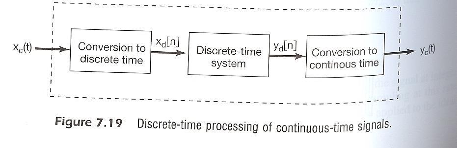
83 Outline 83 Introduction Introduction to filters Representation of a CT Signal by Its Samples: Sampling Reconstruction of a Signal from Its Samples: Interpolation The Effect of Under-sampling: Aliasing Examples o Discrete-Time Processing of Continuous-Time Signals o DT processing: Effective CT Frequency Response o DT from CT: Impulse invariance o CT processing: Effective DT Frequency Response o A/D and D/A Conversion o Sampling of Discrete-Time Signals o Quantization o Summary

84 84 DT Processing; CT Processing otherwise 0 ; T e H j H j eff otherwise 0 ; T j H e H c j

85 DT Processing of CT Signals Reason for this: We can take advantage of the vast variety of general- or special-purpose discrete time signal processing devices (t) x c C/D Conversion xd[ n] xc ( nt) y [ n] y ( nt) d c D/C DT-S Conversion y c (t) x d T [ n] x ( nt) c y d T [ n] y ( nt) c 85

86 DT Processing of CT Signals 86 Overall system is equivalent to a CT system: Input and output are CT The CT system depends on Discrete-time system Sampling rate What is the equivalent (effective) frequency response of the overall system? 1. Find the relation between x c (t) and x[n] 2. Next between y[n] and x[n] 3. Finally between y r (t) and y[n] H eff j H e 0 j ; T otherwise

87 C/D Conversion Fig

88 88 C/D Conversion Illustration in the Frequency Domain

89 C/D Conversion Illustration in the Frequency Domain CT x t x t st x t t nt x nt t nt s c n c n c X s 1 T j X j k k c s n x c ( nt) e j nt Periodic with period 2 s T 89

90 C/D Conversion Illustration in the Frequency Domain DT j n j n Xd e j e xd n x nt e ( ) [ ] ( ) c n n Periodic with period N=2Π = CT frequency T = DT frequency ( ) 90

91 D/C Conversion y d [n] y c (t) Reverse of the process of C/D conversion 91

92 C/D & D/C conversion Effective Frequency Response 92 So what is the frequency response of the overall system First step is the relation between x c (t) and x[n] Next between y[n] and x[n] Finally between y r (t) and y[n] H eff j H e 0 j ; T otherwise

93 93 Effective Frequency Response Input CT to DT Assume a DT LTI system Output DT to CT Output frequency response Effective Frequency Response k c j T k 2 T j X T 1 X e nt x n x c k c j j j j T k T j X e H T e X e H e Y 2 1 n r / T nt t / T nt t sin y n t y otherwise 0 / T TY e j Y T j r otherwise 0 / T j X H e j Y c T j r otherwise 0 / T H e j H T j eff j X j H j Y c eff r

94 Example 4.3 (DTSP): Ideal low-pass filter implemented as a DT system CT input signal Sampled CT input signal Apply DT LPF 94

95 Example 4.3: Ideal low-pass filter implemented as a DT system Signal after DT LPF is applied Application of reconstruction filter Output CT signal after reconstruction 95

96 Freq. response of Differentiator 96

97 Freq. response of integrator 97

98 Example 4.4: Digital Differentiator Construction of Band-limited Digital Differentiator Desired: Hc( j) j c c Set s 2 c T 2 s c M c 98

99 99 Example 4.4: Digital Differentiator

100 100 Example: Problem 7.29 S&S

101 Outline 101 Introduction Introduction to filters Representation of a CT Signal by Its Samples: Sampling Reconstruction of a Signal from Its Samples: Interpolation The Effect of Under-sampling: Aliasing o Discrete-Time Processing of Continuous-Time Signals o DT processing: Effective CT Frequency Response o DT from CT: Impulse invariance o CT processing: Effective DT Frequency Response o A/D and D/A Conversion o Sampling of Discrete-Time Signals o Quantization o Summary

102 Impulse Invariance Impulse Invariance: The sampling of the CT impulse response h(t) to produce the DT impulse response h[n] If h(t) is appropriately band-limited j H( e ), the frequency response of the DT system will be defined as H( j) the CT system's frequency response with linearly-scaled frequency i.e., If the CT filter has poles at s = sk, these poles are translated to poles at ; T is sampling period if the CT filter is causal and stable, then the DT filter will be causal and stable as well 102

103 Impulse Invariance Given a CT system H c (j) how to choose DT system response H(e j ) so that effective response of DT system H eff (j)=h c (j) Answer: H j e H j /T c Condition: H c j 0 / T Given these conditions, the DT impulse response can be written in terms of CT impulse response as hn Th nt c Resulting system is the impulse-invariant version of the CT system 103

104 Example: Impulse Invariance Ideal low-pass DT filter by impulse invariance H c j 1 0 else c The impulse response of CT system is h c t sin t c t Obtain DT impulse response via impulse invariance h n Th nt sin c T nt The frequency response of the DT system is c nt sin n n c 104 H c e j 1 0 c c

105 Outline o o o o o Introduction Introduction to filters Representation of a CT Signal by Its Samples: Sampling Reconstruction of a Signal from Its Samples: Interpolation The Effect of Under-sampling: Aliasing Discrete-Time Processing of Continuous-Time Signals o DT processing: Effective CT Frequency Response o DT from CT: Impulse invariance o CT processing: Effective DT Frequency Response A/D and D/A Conversion Sampling of Discrete-Time Signals Quantization Summary 105

106 CT processing of DT signals H e j H c j 0 ; T otherwise 106

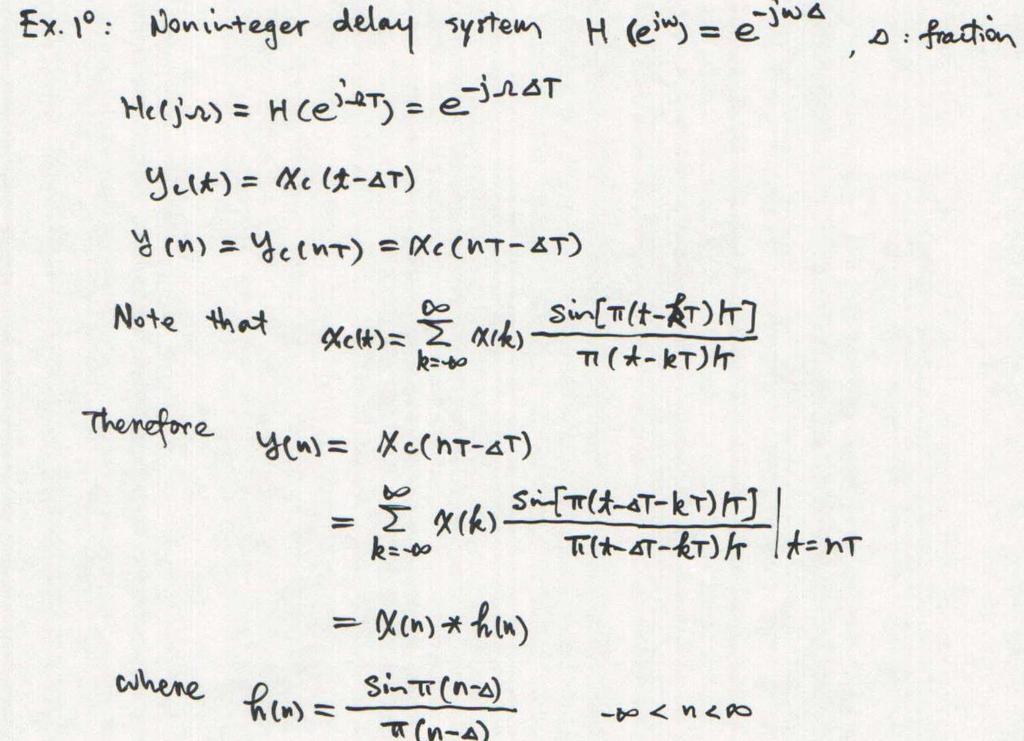
107 Discrete-Time System for Arbitrary Delay y[ n] x[ n H e j H ( z) e z j ; real or integer For integer delay values: This DT system is meaningful: the samples y(n) are equal to the delayed samples of x(n) For real delay values: y(n) would lie somewhere between the known samples of x(n) The unknown y(n) would then have to be obtained by way of interpolation from the known x(n) y[ n] N integer; x[ n k x n sinc( n k); real; T 1sampling period 107 Conclusion: producing a fractional delay requires reconstruction of the discrete-time signal and shifted resampling of the resulting continuous-time (T=1 to simplify notation)

108 108

109 Discrete-Time Moving Average System y[ n] H (e 1 M 1 j ) M k = 0 1 M 1 1 M 1 x [n - k] M k = 0 e - jk sin( ( M 1) / sin( ) 2) e - jm / h[ n] 1, M 1 0, M n 0 otherwise

110 For even M, this moving average will cause a noninteger delay to the input 110

111 Summary o o DT processing: Effective CT Frequency Response DT from CT: Impulse invariance H o Sampling of hc(t) eff j h H e 0 j n Th nt c ; T otherwise o CT processing: Effective DT Frequency Response H e j H c j 0 ; T otherwise 111

112 Outline Introduction Introduction to filters Representation of a CT Signal by Its Samples: Sampling Reconstruction of a Signal from Its Samples: Interpolation The Effect of Under-sampling: Aliasing o Examples o Discrete-Time Processing of Continuous-Time Signals o A/D and D/A Conversion: o o o o Practical sampling & reconstruction Sampling of Discrete-Time Signals Quantization Summary 112

113 A/D and D/A Conversion Ideal impulse sampling Practical rectangular sampling A non-ideal system samples x(t) at a given instant and holds that value until the next instant, at which a sample should be taken 113 x(t) Zero-order hold x 0( t )

114 A/D and D/A Conversion Up to this point we assumed ideal D/C and C/D conversion In practice, CT signals are not perfectly band-limited D/C and C/D converters can only be approximated with D/A and A/D converters A more realistic model for digital signal processing H e j H eff j 114 In the following we discuss each block of this figure

115 1) AntiAliasing filter AAF Desirable 1. to minimize sampling rate: Minimizes amount of data to process 2. to reduce noise: no point of sampling high frequencies that are not of interest (e.g., noise) A low-pass anti-aliasing filter would improve both aspects An ideal anti-aliasing filter AAF The effective response via DT LPF is In practice an ideal AAF is not possible; hence H aa j H eff 1 c / T 0 c j H e 0 H eff jt jt j H jh e aa c c 115 Haa() is a sharp-cutoff analog filters which are expensive

116 Simplifying AAF : Oversampled A/D Conversion 1. have a simple (gradual cutoff) analog anti-aliasing filter 2. use higher than required sampling rate s 2M N T 1 M N 3. implement sharp DT anti-aliasing filter c M 4. downsample to desired sampling rate ' 2 s 2M N/M N 116

117 Oversampled A/D Conversion: simplifying AAF x ( at) X j/ a M Digital Signal Processing

118 2) A/D Conversion Two steps: sampling in time t and quantization of the amplitude x Sampling x[n] = x(nt) Quantization: map amplitude values into a set of discrete values x [n] = Q(x[n]) Quantization error: e[n] = x[n]-x [n] 118

119 2) A/D Conversion Ideal C/D converters convert CT signals into infinite-precision DT signals In practice we implement C/D converters as the cascade of The sample-and-hold device holds current/voltage constant The A/D converter converts current/voltage into finite-precisions number The ideal sample-and-hold device has the output 119 x t xnh t 0 0 nt n h 0 H t 0 ( 1, 0, j) 0 e t else T / 2) jt / 2 2sin( T

120 A/D Conversion : Ideal Sample and Hold x t xnh t 0 0 nt n Time-domain: 120

121 A/D Conversion: Sampling with Zero-Order Hold o Zero-order hold: impulse-train sampling followed by an LTI system with a rectangular impulse response s(t) xs (t) xs (t) x ( t) ( t)* ( t) 0 s 0 x h 121

122 Example: Prob 7.24 S&S Sampling with a square signal 122

123 Outline o o o o o o o o o Introduction Filters for sampling Representation of a CT Signal by Its Samples: Sampling The Effect of Under-sampling: Aliasing Sampling with Zero-Order Hold Reconstruction of a Signal from Its Samples: Interpolation Examples Discrete-Time Processing of Continuous-Time Signals Quantization Sampling of Discrete-Time Signals A/D and D/A Conversion o A/D conversion o D/A conversion Quantization Summary 123

124 3) D/A conversion: Reconstruction Methods Reconstruction: connecting samples x[n] using interpolation kernels a) Zero-Order Hold: D/A Conversion e.g. scanned images b) First-Order Hold: D/A Conversion Linear interpolation: commonly used in plotting x zoh t t x foh 124

125 125 Ideal, zero-order hold, and first-order hold reconstruction

126 D/A Conversion: Zero-Order Hold: Perfect reconstruction requires filtering with ideal LPF The ideal reconstruction filter jt r j X e H r j jt e :DTFTof The time domain reconstructed signal is x r X X X t r H r sampled signal j:ft of reconstructed signal j n T / T 0 / T In practice we cannot implement an ideal reconstruction filter x n sin t t nt / T nt / T 126

127 D/A Conversion: Reconstruction with Zero- Order Hold Zero-order hold T ( j) H r Ideal interpolating filter s s 2 0 s 2 s 127

128 D/A Conversion The practical D/A converter: Digital to analog converter + Analog LPF It takes a binary code and converts it into CT output x ˆ DA m B 0 0 n n t X xˆ n h t nt xnh t nt Using the additive noise model for quantization The signal component in frequency domain can be written as Note: x[n]=xa(nt) jt jt 1 X0j Xe H 0j X e X a j k T k To recover the desired signal component we need a compensated reconstruction filter of the form to get xa(t) back ~ Hr j Hr j H j 128 t x t e t xnh t nt enh t nt xda n n 0 s

129 D/A Conversion: Reconstruction with Zero-Order Hold o Cascade of a zero-order hold with a reconstruction filter x(t) s(t) p(t) xs (t) x p (t) 1 0 T t H( j) h 0( t ) ( ) x 0 t h r (t) ( j) H r xr(t) r(t) 129 H H 0 r 2sin( T jt / 2 ( j) e jt / 2 e H ( j) ( j) 2sin( T / 2) / 2)

130 4) Compensated Reconstruction Filter ~ H The frequency response of zero-order hold is r j H H r 0 j j H 2 sin T / 2 jt / 2 0 j e Therefore the compensated reconstruction filter should be ~ H r j sin T / 2 T / 2 0 e jt / 2 / T / T 130

131 D/A Conversion: Reconstruction with Zero- Order Hold Reconstruction filter H r ( j) ( j) H r s 2 s 2 s 2 s 2 Magnitude and phase for the reconstruction filter for a zero-order hold 131

132 First-Order Hold: Linear interpolation Impulse-train sampling followed by convolution with a triangular impulse response n s ( t) ( t nt ) xs(t) x (t) [n] xs ( j ) H r 132

133 First-Order Hold: Linear interpolation s(t) x[n] xs(t) xs(t) 133

134 First-order versus zero-order hold First-order hold filter: the signal is reconstructed as a piecewise linear approximation to the original signal xc(t) h(t) is a triangle Zero-order hold filter converts a DT signal to a CT signal by holding each sample value for one sample interval h(t) is a square 134

135 Comparison of frequency responses of ideal lowpass, zeroorder hold, and first-order hold reconstruction filters zero-order since the CT signal is a zeroth order polynomial between the sampling points first-order since the CT signal is a first order polynomial between the sampling points 135

136 Sampling and Interpolation of Images 136 Fig & Fig 7.14

137 Outline Introduction Introduction to filters Representation of a CT Signal by Its Samples: Sampling Reconstruction of a Signal from Its Samples: Interpolation The Effect of Under-sampling: Aliasing o Discrete-Time Processing of Continuous-Time Signals o A/D and D/A Conversion o Sampling of Discrete-Time Signals: o Up-Sampling (more samples) o Down-sampling (less samples) o o 137 Quantization Summary

138 Up & Down Sampling: Applications 138 Sampling-rate conversion: Given a digital signal, change its sampling rate Necessary for image display when original image size differs from the display size Necessary for converting speech, audio, image, video from one format to another Sometimes we reduce sample rate to reduce the data rate Down-sampling: reduce the sampling rate Up-Sampling: increase the sampling rate Audio CD Film DVD TV Signal Underwater signal Upsampling

139 Recall: Time-Scaling of signals x(at) x(t) x(2t) Ex: Upsampling Compression a>1 x(t/2) Linearly stretching a<1 Ex: Downsampling 139

140 Down-Sampling of DT Signals Impulse-Train Sampling x[n] xp[n] 140 x p [ ] p n [ n kn] k x[ n], [ n] 0, x [ n] x[ n] p[ n] p k N sampling period if n=an integer multiple of N otherwise x[ kn] [ n kn ]

141 Down-Sampling of DT Signals Time domain illustration by a factor of 2 x[n] n p[n] n xp[n] n 141 Fig. 7.31

142 X j 2 P ( e ) ( ks ) N X p ( e j Down-Sampling of DT Signals Frequency domain analysis 1 2 j j j( ) p ( e ) P( e ) X ( e ) 2 ) 1 N k N 1 k0 X ( e d j( k ) s ) 2 2 Aliasing 1 X ( e M 0 M 2 N 1 N P( e j X p( e M 0 M 1 N j ) ) s j ) s s ( M ) 2 2 s 2 M 2 s 2 M 142 Fig s 0 2

143 Down-Sampling of DT Signals Exact Recovery Using Ideal Lowpass Filter: 143 Fig 7.33

144 Down-Sampling of DT Signals DT Decimation & Interpolation DT Sampling Decimation 144 Fig. 7.34

145 Down-Sampling of DT Signals Frequency domain illustration of the relationship between DT Sampling and decimation j j/ N Xb( e ) X p( e ) j Xe ( ) Xb ( e j ) X P ( e j ) 145 Fig. 7.35

146 Up-Sampling of DT Signals Higher Equivalent Sampling Rate 146 Fig. 7.37

147 Up-Sampling of DT Signals Spectra for upsampling by a factor of 2 Fig

148 Example: Ex. 7.5 S&S Down-sampling + up-sampling

149 Example: Ex. 7.5 S&S Down-sampling + up-sampling Fig. 7.38

150 Sampling of Discrete-Time Signals: Changing Sampling Rate (Integer Factor) A CT signal can be represented by its samples as n x nt Some applications require us to change the sampling rate Or to obtain a new DT representation of the same CT signal of the form x' The problem is to get x [n] given x[n] x n x nt' where T T' c c Changing the time axis One way of accomplishing this is to Reconstruct the CT signal from x[n] Re-sample the CT signal using new rate to get x [n] This requires analog processing which is often undesired 150

151 Sampling of Discrete-Time Signals Decreasing the Sampling Rate by Integer Factor: Down-Sampling/Decimation We reduce the sampling rate of a sequence by sampling it x d n xnm x nmt This is accomplished with a sampling rate compressor c There will be no aliasing if ' s 2 T' 2 MT 2 N ' s MT N 151 Note that we may obtain x d n by reconstructing the signal and re-sampling it with T =MT

152 Sampling of Discrete-Time Signals Frequency domain analysis of Down Sampling Recall the DTFT of x[n]=x c (nt) The DTFT of the down-sampled signal can similarly written as With r=i+km, And finally k c j T k T j X T e X 2 1 r c r c j d MT r MT j X MT T r T j X T e X 2 1 ' 2 ' ' M i r c j d MT i T k MT j X T M e X M i M i M j j d e X M e X M copies of X(e^jw), frequency-scaled by M and shifted by multiple of 2

153 Frequency domain analysis of Down sampling: No aliasing frequency-scaled by M Normalized freq : T ' TM 153

154 154 Down-sampling Down-sampling 1) expands each 2π-periodic repetition of X(e^jw) by a factor of M along the ω axis new period is then M2π 2) reduces the gain by a factor of M If x[n] is not bandlimited to π/m, aliasing may result from spectral overlap ) ( j j j d e X e X e X

155 Frequency domain analysis of Down sampling: No aliasing Downsampling stretches the DTFT by a factor of M along with the ω axis frequency-scaled by M shifted by multiple of 2 + reduces the gain by M 155 If x[m] is not band limited to π/m aliasing Source:

156 156 Downsampling without filtering (causes aliasing) and with filter

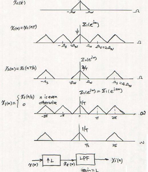
157 Sampling of Discrete-Time Signals Increasing the Sampling Rate by Integer Factor: Up-sampling/Interpolation Increase the sampling rate of a sequence by interpolating it Sampling rate expander x n xn / L x nt L i c / We obtain x i [n] that is identical to what we would get by reconstructing the signal and re-sampling it with T =T/L 157 Up sampling consists of two steps: Expanding & Interpolating x e n x n / L 0 n 0, L, 2L,... else k x k n kl

158 158

159 Sampling of Discrete-Time Signals: Expanding The DTFT of x e [n] can be written as X e j jn jlk jl e x k n kl e x k e X e n k k The output of the expander is frequency-scaled 159

160 Interpolating sampled DT signals The DTFT of the desired interpolated signals is The extrapolator output is given as To get interpolated signal we apply the following ideal LPF 160

161 Upsampling: insertion of L 1 zeros between every sample of the input signal Upsampling compresses the DTFT by a factor of L along with the ω axis 161

162 Interpolator in Time Domain x i [n] in a low-pass filtered version of x[n] The low-pass filter impulse response is sin n / L h n i n / L Hence the interpolated signal is written as Note that h h i i 0 n 1 x i n k 0 n L, 2L,... x k sin n kl / L n kl / L 162 the filter output can be written as x i n xn / L x nt / L x nt' for n 0, L, 2L,... c c

163 Non-ideal LPF: Linear interpolation 163

164 Sampling of Discrete-Time Signals: Changing the Sampling Rate by Non-Integer Factor: combine decimation and interpolation Since both interpolation and anti-aliasing filters are low-pass filters, the filter with the smallest bandwidth is more restrictive and can therefore be used in place of both filters 164

165 Sampling of Discrete-Time Signals: Changing the Sampling Rate by Non-Integer Factor If M>L: net increase of sampling period (or decrease in sampling frequency) net operation is downsampling π / M is the dominant cutoff frequency & the low-pass filter should have cutoff at π / M If M<L and T respects Nyquist theorem π / L is the dominant cutoff frequency no need to further limit the bandwidth of the signal below Nyquist frequency 165 Interpolation and downsampling are not reversible, due to loss of data

166 166 Changing the rate by 2/3

167 Outline Introduction Filters for sampling Representation of a CT Signal by Its Samples: Sampling The Effect of Under-sampling: Aliasing o Reconstruction of a Signal from Its Samples: Interpolation o Discrete-Time Processing of Continuous-Time Signals o A/D and D/A Conversion o Sampling of Discrete-Time Signals o Quantization o Summary 167

168 Quantization C/D converter can be modeled as Quantizer transforms input into a finite set of numbers Most of the time uniform quantizers are used Quantization is the process of approximating ("mapping") a continuous set of values by a relatively small ("finite") set of discrete symbols or integer values For example, rounding a real number in the interval [0,100] to an integer (a continuous set or a very large set of possible discrete values) (to discrete values or to values which can still take on continuous range) Quantization can be described as a mapping that represents a finite continuous interval I = [a,b] of the range of a continuous valued signal, with a single number c, which is also on that interval xˆ n Q x n 168

169 Quantization xˆ n The step-size Q depends on Q x n the dynamic range of the signal amplitude and perceptual sensitivity The signal range D (or also Xm) & step-size Q determine the bitrate R bits/sample 2^B=D/Q Q=Xm/2^B For speech: B = 8 bits; For music: B =16 bits One can trade off T (or fs) and Q (or B): lower B -> higher fs; higher B -> lower fs 169

170 Uniform Quantizer Applicable when the signal is in a finite range (fmin, fmax) The entire data range is divided into L equal intervals of length Q Q=(fmax-fmin)/L Q quantization interval or quantization step-size Interval i is mapped to the middle value of this interval We store/send only the index of quantized value Index of quantized value Qi(f) = f-fmin/q Quantized value Q(f) = Qi(f)*Q +Q/2+fmin 170 Source:

171 Uniform Quantizer: Example 171 Source:

172 Quantization: applications Telephony system: 8-bit quantization Values of the analog sound are rounded to the closest of 256 distinct voltage values represented by an 8-bit binary number This causes quantization noise into the signal, but the result is still more than adequate to represent human speech Music: CDs use 16-bit quantization: allowing 65,536 distinct voltage levels 172 Image processing: lossy compression achieved by quantization or compressing a range of values to a single quantum value For example, reducing the number of colors required to represent a digital image Ex: DCT data quantization in JPEG

173 173 Audio Quantization

174 Effect of Quantization Step-size: quantization noise/error 174 Source:

175 Quantization Error n xˆ n xn Quantization error: difference between the original and quantized value If quantization step is, the quantization error will satisfy / 2 / 2 e n if the input does not clip we may use the following simplified model e 175 ( Xm / 2) x[ n] ( Xm / 2)

176 Quantization Error e n xˆ n xn In most cases we can assume that e[n] is uniformly distributed random variable Is uncorrelated with the signal x[n] e[n] is Gaussian white noise The variance of e[n] is then 2 2 e 12 The signal-to-noise ratio SNR of e[n] for B+1 bits SNR 6.02 B log 10 x SNR is proportional to the bitrate B X m 176

177 Derivation of e[n]: Assume x[n] is bipolar, i.e., varying in [-A A] 177

178 Measuring Quantizer Performance Performance measure: how close the quantized signal (e.g., sound) to the original signal to the human ears - Perceptual Quality No objective measure correlates very well with the perceptual quality Frequently used objective measure: mean square error (MSE) between original and quantized samples or signal to noise ratio 178

179 Problems with uniform quantization Only optimal for uniformly distributed signal Real audio signals (speech and music) are more concentrated near zeros Human ear is more sensitive to quantization errors at small values Solution: Using non-uniform quantization quantization interval is smaller near zero 179

180 Quantizer & coder 180 Xm signal range

181 Quantizer & coder Two s Complement Numbers 181 Representation for signed numbers in computers B B Integer two s-complement a 2 a12 0 Fractional two s-complement a 2 a 2 Example B+1=3 bit two s-complement numbers ab 2 1 B ab 2 -a a a a a a Binary Symbol Numerical Value Binary Symbol Numerical Value / / / / / / /4

182 182 Example

183 Outline Introduction Filters for sampling Representation of a CT Signal by Its Samples: Sampling The Effect of Under-sampling: Aliasing o Sampling with Zero-Order Hold o Reconstruction of a Signal from Its Samples: Interpolation o Examples o Discrete-Time Processing of Continuous-Time Signals o Sampling of Discrete-Time Signals o A/D and D/A Conversion o Summary 183

184 Summary The information carried by a signal can be defined either in terms of its Time Domain pattern or its Frequency Domain spectrum The amount of information in a continuous analog signal x(t) can be specified by a finite number of values: samples x[n] The Sampling Theorem states that we can collect all the information in a signal by sampling at a rate 2xωm, where ωm is the signal bandwidth of x(t) We can, therefore, reconstruct the actual shape of the original continuous signal at any instant in between the sampled instants This reconstruction is not a guess but a true reconstruction 184

185 Summary The FT of a DT signal is a function of the continuous variable ω, and it is periodic with period 2π Given a value of ω, the FT gives back a complex number that can be interpreted as magnitude and phase (translation in time) of the sinusoidal component at that frequency ω Sampling is a multiplication with a periodic impulse train FT of sampled signal: original FT + shifted versions at multiples of ωs Sampling the CT signal x(t) with interval T, we get the DT signal x[n]=x[nt] which is a function of the discrete variable n Sampling a CT signal with sampling rate fs produces a DT signal whose FT is the periodic replication of the original signal, and the replication period is Ts The Fourier variable ω for functions of discrete variable is converted into the frequency variable f (in Hertz) by means of f=ω/(2πt) 185

186 Summary A-to-D converters convert CT signals into sequences with discrete sample values Operates with the use of sampling and quantization D-to-A converters convert sequences with discrete sample values into continuous-time signals Analyzed as conversion to impulse train followed by reconstruction filtering Zero-order hold is a simple but low performance filter Upsampling and downsampling allow for changes in the effective sample rate of sequences Allows matching of sample rates of A-to-D, D-to-A, and digital processor Analysis: downsampler/upsampler similar to A-to-D/D-to-A When performing a frequency-domain analysis of systems with up/downsamplers, it is strongly recommended to carry out the analysis in the z-domain until the last step Working directly in the ω domain can easily lead to errors 186

187 Summary: to know.. How the sampling is derived using the FT.. Lowpass filters for reconstruction.. The sampled signal spectrum contains the original spectrum and its replicas (aliases) at kws, k=+/- 1,2,. We need a prefilter when sampling a signal To avoid aliasing The filter should be a lowpass filter with cutoff frequency at fs /2 Sample-and-hold and linear interpolation Why the ideal interpolation filter is a lowpass filter with cutoff frequency at fs/2 The ideal interpolation kernel is the sinc function. Why to apply a pre-filter before sampling. 187