Fourier PCA. Navin Goyal (MSR India), Santosh Vempala (Georgia Tech) and Ying Xiao (Georgia Tech)

Transcription

1 Fourier PCA Navin Goyal (MSR India), Santosh Vempala (Georgia Tech) and Ying Xiao (Georgia Tech)

2 Introduction 1. Describe a learning problem. 2. Develop an efficient tensor decomposition.

3 Independent component analysis See independent samples x = As: s R m is a random vector with independent coordinates. Variables s i are not Gaussian. A R n m is a fixed matrix of full row rank. Each column A i R m has unit norm. Goal is to compute A.

4 ICA: start with independent random vector s

5 ICA: independent samples

6 ICA: but under the map A

7 ICA: goal is to recover A from samples only.

8 Applications Matrix A gives n linear measurements of m random variables. General dimensionality reduction tool in statistics and machine learning [HTF01]. Gained traction in deep belief networks [LKNN12]. Blind source separation and deconvolution in signal processing [HKO01]. More practically: finance [KO96], biology [VSJHO00] and MRI [KOHFY10].

9 Status Jutten and Herault 1991 formalised this problem. Studied in our community first by [FJK96]. Provably good algorithms: [AGMS12] and [AGHKT12]. Many algorithms proposed in signals processing literature [HKO01].

10 Standard approaches PCA Define a contrast function where optima are A j. Second moment E ( (u T x) 2) is usual PCA. Only succeeds when all the eigenvalues of the covariance matrix are different. Any distribution can be put into isotropic position.

11 Standard approaches fourth moments Define a contrast function where optima are A j. Fourth moment E ( (u T x) 4). Tensor decomposition: T = m λ j A j A j A j A j j=1 In case A j are orthonormal, they are the local optima of: T (v, v, v, v) = T ijkl v i v j v k v l where v = 1. i,j,k,l

12 Standard assumptions for x = As All algorithms require: 1. A is full rank n n: as many measurements as underlying variables. 2. Each s i differs from a Gaussian in the fourth moment: E (s i ) = 0, E ( si 2 ) ( ) = 1, E s 4 i 3 Note: this precludes the underdetermined case when A R n m is fat.

13 Our results We require neither standard assumptions. Underdetermined: A R n m is a fat matrix where n << m. Any moment: E (s r i ) E (zr ) where z N(0, 1). Theorem (Informal) Let x = As be an underdetermined ( )] m ) ICA model. Let d 2N be such that σ m ([vec > 0. Suppose for each s i, one A d/2 i i=1 of its first k cumulants satisfies cum ki (s i ). Then one can recover the columns of A up to ɛ accuracy in polynomial time.

14 Underdetermined ICA: start with distribution over Rm

15 Underdetermined ICA: independent samples s

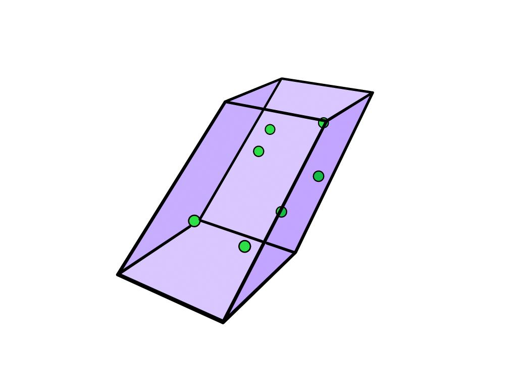
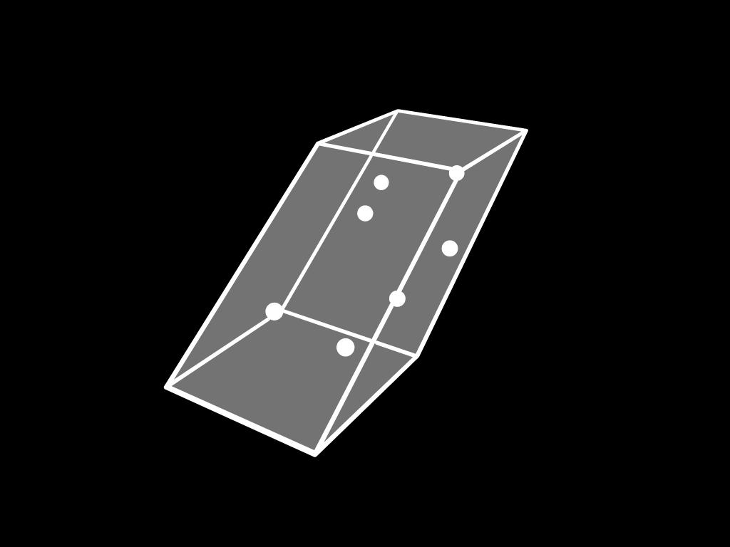
16 Underdetermined ICA: A first rotates/scales

17 Underdetermined ICA: then A projects down to Rn

18 Fully determined ICA nice algorithm 1. (Fourier weights) Pick a random vector u from N(0, σ 2 I n ). For every x, compute its Fourier weight w(x) = e iut x x S eiut x. 2. (Reweighted Covariance) Compute the covariance matrix of the points x reweighted by w(x) µ u = 1 S x S w(x)x and Σ u = 1 S 3. Compute the eigenvectors V of Σ u. w(x)(x µ u )(x µ u ) T. x S

19 Why does this work? 1. Fourier differentiation/multiplication relationship: (f )ˆ(u) = (2πiu)ˆf (u) 2. Actually we consider the log of the fourier transform: ( ( )) ( ) D 2 log E exp(iu T x) = Adiag g j (A T j u) where g j (t) is the second derivative of log(e (exp(its j ))). A T

20 Technical overview Fundamental analytic tools: Second characteristic function ψ(u) = log(e ( exp(iu T x) ). Estimate order d derivative tensor field D d ψ from samples. Evaluate D d ψ at two randomly chosen u, v R n to give two tensors T u and T v. Perform a tensor decomposition on T u and T v to obtain A.

21 First derivative Easy case A = I n : Thus: ψ u 1 = = ψ(u) = log(e ( ) ( ) exp(iu T x) = log(e exp(iu T s) 1 ( ) E (exp(iu T s)) E s 1 exp(iu T s) 1 n j=1 E (exp(iu js j )) E (s 1 exp(iu 1 s 1 )) = E (s 1 exp(iu 1 s 1 )) E (exp(iu 1 s 1 )) n E (exp(iu j s j )) j=2

22 Second derivative Easy case A = I n : 1. Differentiating via quotient rule: 2 ψ u Differentiating a constant: = E ( s 2 1 exp(iu 1s 1 ) ) E (s i exp(iu 1 s 1 )) 2 E (exp(iu 1 s 1 )) 2 2 ψ u 1 u 2 = 0

23 General derivatives Key point: taking one derivative isolates each variable u i. Second derivative is a diagonal matrix. Subsequent derivatives are diagonal tensors: only the (i,..., i) term is nonzero. NB: Higher derivatives are represented by n n tensors. There is one such tensor per point in R n.

24 Basis change: second derivative When A I n, we have to work much harder: ( ) D 2 ψ u = Adiag g j (A T j u) where g j : R C is given by: A T g j (v) = 2 v 2 log (E (exp(ivs j)))

25 Basis change: general derivative When A I n, we have to work much harder: D d ψ u = m g(a T j u)(a j A j ) j=1 where g j : R C is given by: g j (v) = d v d log (E (exp(ivs j))) Evaluating the derivative at different points u give us tensors with shared decompositions!

26 Single tensor decomposition is NP hard Forget the derivatives now. Take λ j C and A j R n : T = m λ j A j A j, j=1 When we can recover the vectors A j? When is this computationally tractable?

27 Known results When d = 2, usual eigenvalue decomposition. M = n λ j A j A j j=1 When d 3 and A j are linearly independent, a tensor power iteration suffices [AGHKT12]. T = m λ j A j A j, j=1 This necessarily implies m n. For unique recovery, require all the eigenvalues to be different.

28 Generalising the problem What about two equations instead of one? T µ = m µ j A j A j T λ = j=1 m λ j A j A j j=1 Our technique will flatten the tensors: M µ = [ ( vec A d/2 j )] [ ( diag (µ j ) vec A d/2 j )] T

29 Algorithm Input: two tensors T µ and T λ flattened to M µ and M λ : 1. Compute W the right singular vectors of M µ. 2. Form matrix M = (W T M µ W )(W T M λ W ) Eigenvector decomposition M = PDP For each column P i, let v i C n be the best rank 1 approximation to P i packed back into a tensor. 5. For each v i, output re ( e iθ v i ) / re ( e iθ v i ) where θ = argmax θ [0,2π] ( re ( e iθ v i ) ).

30 Theorem Theorem (Tensor decomposition) Let T µ, T λ R n n be order d tensors such that d 2N and: ( where vec µ i λ i T µ = A d/2 j m j=1 µ j A d j T λ = m j=1 λ j A d j ) are linearly independent, µ i /λ i 0 and µ j λ j > 0 for all i, j. Then, the vectors Aj can be estimated to any desired accuracy in polynomial time.

31 Analysis Let s pretend M µ and M λ are full rank: [ ( M µ M 1 λ = vec = A d/2 j ( [ ( vec [ ( vec A d/2 j )] [ ( diag (µ j ) vec A d/2 j )] A d/2 j )] T )] T ) 1 diag (λ j ) 1 [ vec ( [ ( diag (µ j /λ j ) vec A d/2 j )] 1 The eigenvectors are flattened tensors of the form A d/2 j. A d/2 j )] 1

32 Diagonalisability for non-normal matrices When can we write A = PDP 1? Require all eigenvectors to be independent (P invertible). Minimal polynomial of A has non-degenerate roots.

33 Diagonalisability for non-normal matrices When can we write A = PDP 1? Require all eigenvectors to be independent (P invertible). Minimal polynomial of A has non-degenerate roots. Sufficient condition: all roots are non-degenerate.

34 Perturbed spectra for non-normal matrices More complicated than normal matrices: Normal: λ i (A + E) λ i (A) E. not-normal: Either Bauer-Fike Theorem λ i (A + E) λ j (A) E for some j, or we must assume A + E is already diagonalizable. Neither of these suffice.

35 Generalised Weyl inequality Lemma Let A C n n be a diagonalizable matrix such that A = Pdiag (λ i ) P 1. Let E C n n be a matrix such that λ i (A) λ j (A) 3κ(P) E for all i j. Then there exists a permutation π : [n] [n] such that λi (A + E) λ π(i) (A) κ(p) E. Proof. Via a homotopy argument (like strong Gershgorin theorem).

36 Robust analysis Proof sketch: 1. Apply Generalized Weyl to bound eigenvalues hence diagonalisable. 2. Apply Ipsen-Eisenstat theorem (generalised Davis-Kahan sin(θ) theorem). ( 3. This implies that output eigenvectors are close to vec 4. Apply tensor power iteration to extract approximate A j. A d/2 j 5. Show that the best real projection of approximate A j is close to true. )

37 Underdetermined ICA Algorithm x = As where A is a fat matrix. 1. Pick two independent random vectors u, v N(0, σ 2 I n ). 2. Form the d th derivative tensors at u and v, T u and T v. 3. Run tensor decomposition on the pair (T u, T v ).

38 Estimating from samples [D 4 ψ u ] i1,i 2,i 3,i 4 = 1 [ ( ) φ(u) 4 E (ix i1 )(ix i2 )(ix i3 )(ix i4 ) exp(iu T x) φ(u) 3 ( ) ( ) E (ix i2 )(ix i3 )(ix i4 ) exp(iu T x) E (ix i1 ) exp(iu T x) φ(u) 2 ( ) ( ) E (ix i2 )(ix i3 ) exp(iu T x) E (ix i1 )(ix i4 ) exp(iu T x) φ(u) 2 ( ) ( ) E (ix i2 )(ix i4 ) exp(iu T x) E (ix i1 )(ix i3 ) exp(iu T x) φ(u) 2 + At most 2 d 1 (d 1)! terms. Each one is easy to estimate empirically!

39 Theorem Theorem Fix n, m N such that n m. Let x R n be given by an underdetermined ( )] ICA m model ) x = As. Let d N such that and σ m ([vec > 0. Suppose that for each s i, one of its A d/2 i i=1 cumulants ( d < k i k satisfies cum ki (s i ) and E s i k) M. Then one can recover the columns of A up to ɛ accuracy in time and sample complexity ([ ( )]) ) k poly (n d+k, m k2, M k, 1/ k, 1/σ m vec, 1/ɛ. A d/2 i

40 Analysis Recall our matrices were: [ ( )] M u = vec where: A d/2 i ( ) [ ( diag g j (A T j u) vec g j (v) = d v d log (E (exp(ivs j))) A d/2 i Need to show that g j (A T j u)/g j (A T j v) are well-spaced. )] T

41 Truncation Taylor series of second characteristic: k i g i (u) = cum l (s i ) (iu)l d (l d)! + R (iu) k i d+1 t (k i d + 1)!. l=d Finite degree polynomials are anti-concentrated. Tail error is small because of existence of higher moments (in fact one suffices).

42 Tail error g j is the d th derivative of log(e ( exp(iu T s) ) ). For characteristic function φ (d) (u) ( E x d). Count the number of terms after iterating quotient rule d times.

43 Polynomial anti-concentration Lemma Let p(x) be a degree d monic polynomial over R. Let x N(0, σ 2 ), then for any t R we have Pr ( p(x) t ɛ) 4dɛ1/d σ 2π

44 Polynomial anti-concentration Proof. 1. For a fixed interval, a scaled Chebyshev polynomial has smallest l norm (order 1/2 d when interval is [ 1, 1]). 2. Since p is degree d, there are at most d 1 changes of sign, hence only d 1 intervals where p(x) is close to any t. 3. Applying the first fact, each interval is of length at most ɛ 1/d, each has Gaussian measure 1/σ 2π.

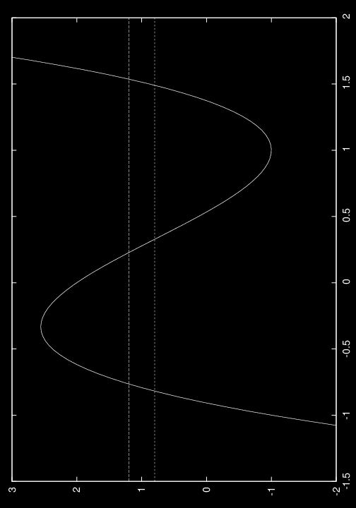
45 Polynomial anti-concentration

46 Eigenvalue spacings ( g Want to bound Pr i (A T i u) g i (A T i v) g j (A T j u) g j (A T j v) Condition on a value of A T j u = s. Then: ). ɛ g i (A T i u) g i (A T i v) s g j (A T j v) = p i (A T i u) g i (A T i v) + ɛ i g i (A T i v) s g j (A T j v) p i (A T i u) g i (A T i v) s g j (A T j v) ɛ i g i (A T i v). Once we ve conditioned on A T j u we can pretend A T i u is also a Gaussian (of highly reduced variance).

47 Eigenvalue spacings A T i u = A i, A j A T j u + r T u where r is orthogonal to A i Variance of remaining ( randomness )]) is r 2 σ m ([vec. A d/2 i We conclude by union bounding with the event that denominators are not too large, and then over all pairs i, j.

48 Extensions Can remove Gaussian noise when x = As + η and η N(µ, Σ). Gaussian mixtures (when x n i=1 w in(µ i, Σ i )), in the spherical covariance setting. (Gaussian noise applies here too.)

49 Open problems What is the relationship between our method and kernel PCA? Independent subspaces. Gaussian mixtures: underdetermined and generalized covariance case.

50 Fin Questions?