B5.6 Nonlinear Systems

Transcription

1 B5.6 Nonlinear Systems 1. Linear systems Alain Goriely 2018 Mathematical Institute, University of Oxford

2 Table of contents 1. Linear systems 1.1 Differential Equations 1.2 Linear flows 1.3 Linear maps 1

3 What you (should) know from previous courses. Phase plane analysis for two-dimensional continuous systems ẋ = f (x, y) (1) ẏ = g(x, y) (2) Poincaré-Bendixson theorem (fixed points, periodic orbits, homo/heteroclinic orbits) Basic linear algebra (eigenvalues, diagonalisation,...) 2

4 1. Linear systems

5 1. Linear systems 1.1 Differential Equations

6 The problem Consider the linear, autonomous, first-order system of differential equations: {ẋ dx dt = Ax x(0) = x 0 (3) where A M n (R). NB: M n (R) is the set of n n matrices with coefficients in R. Questions: Find the solution Describe the behaviour of the solution close to the fixed point x = 0. 3

7 The matrix exponential Definition 1.1 Let A M n (R), t R, then the matrix exponential is e ta = k=0 t k A k. (4) k! This series is absolutely, uniformly convergent for all t < T. Theorem 1.2 The initial value problem (IVP) has the unique solution {ẋ dx dt = Ax x(t 0 ) = x 0 (5) x(t) = e (t t0)a x(t 0 ). (6) 4

8 The matrix exponential Property: If A = BCB 1, then e ta = Be tc B 1. In particular, if A is semi-simple (i.e. A can be diagonalised), then there exists B such that A = BCB 1, where C = diag(λ 1,..., λ n ), (7) therefore e ta = Bdiag(e λ1t,..., e λnt )B 1 (8) 5

9 2D Example If A M 2 (R), the system is {ẋ1 = a 11 x 1 + a 12 x 2 ẋ 2 = a 21 x 1 + a 22 x 2 (9) where a ij R. Let A = (a ij ) and B GL(2, R). (NB: GL(n, R) is the group of n n invertible matrices with real coefficients) Then y = Bx transforms the system ẋ = Ax into ẏ = Cy, where C = BAB 1. (10) Depending on the eigenvalues λ 1, λ 2 Spec(A) (the spectrum of A), we can choose B such that C has one of the following forms 6

10 2D Example 7

11 2D Example 1 λ 1, λ 2 R 1.1 SADDLE: λ 1λ 2 < 0 8

12 2D Example 1 λ 1, λ 2 R 1.2 NODE: λ 1λ 2 > 0 with A semi-simple (i.e. with 2 different eigenvectors). 9

13 2D Example 1 λ 1, λ 2 R 1.3 DEGENERATE NODE: λ 1 = λ 2 = λ with A not semi-simple (i.e. there exists, up to a multiplicative constant, 1! eigenvector). 10

14 2D Example 2 λ 1, λ 2 C, λ 1 = a + ib (a, b real). 2.1 CENTRE: a = 0 11

15 2D Example 2 λ 1, λ 2 C, λ 1 = a + ib (a, b real). 2.2 FOCUS: a 0 12

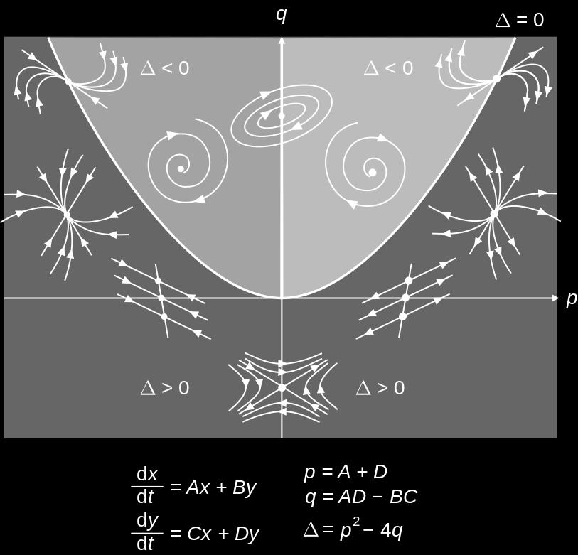
16 2D Example 13

17 1. Linear systems 1.2 Linear flows

18 Linear flows Consider ẋ = Ax, x(t 0 ) = x 0. x R, A M n (R), n 1. The general solution is x(t) = e ta x 0. Geometrically, e ta is a map, the linear flow: Properties: ϕ t = e ta : R n R n (11) x(t) = ϕ t (x 0 ) (12) ϕ 0 = 1 (the identity map) ϕ t+s (x) = ϕ t (ϕ s (x)) = ϕ s (ϕ t (x)), x R n 14

19 Hyperbolic flows Consider the set of eigenvalues of A: Spec(A) = {λ 1,..., λ n } (13) Definition 1.3 If A is such that Re(λ) 0, λ Spec(A), then the linear flow e ta is hyperbolic. By extension, the system ẋ = Ax is a hyperbolic system. NB: Since the real part of all the eigenvalues are all different from zero, hyperbolic flows are controlled by exponential contraction or expansion close to the fixed point. 15

20 Invariant sets Consider the set of eigenvalues of A: Spec(A) = {λ 1,..., λ n } (14) Definition 1.4 Let E R n. Then E is an invariant set of ϕ if ϕ t (E) E t R. Example: Let v be an eigenvector of A with eigenvalue λ, then E = Span(v) is an invariant set. Proof: 16

21 Linear subspaces We build different invariant sets based on the real part of the spectrum. First, consider the case where A is semi-simple and Spec(A) = {λ 1,..., λ n }. We write the eigenvalues and eigenvectors of A as { λj = a j + ib j, j = 1,..., n We have Aw j = λ j w j,. w j = u j + iv j, j = 1,..., n (15) Definition 1.5 The stable, center, unstable linear subspaces are defined, respectively, as E s = Span(u j, v j j s.t. a j < 0) E c = Span(u j, v j j s.t. a j = 0) E u = Span(u j, v j j s.t. a j > 0) (stable linear subspace) (centre linear subspace) (unstable linear subspace) 17

22 Linear subspaces Define n s = dim(e s ) n c = dim(e c ) n u = dim(e u ) then n = n s + n c + n u. By construction E s, E c, and E n are invariant sets In the case where the unstable and centre subspaces are empty, we have: PROPERTY: If all the eigenvalues have negative real part, then x 0 R n, the origin is stable. That is, we have lim t eta x 0 = 0 (16) and x 0 0 lim t eta x 0 = (17) NB: This property remains true x 0 E s. 18

23 Linear subspaces If A is not semi-simple, then we take w j to be the generalized eigenvectors (See Perko, p.33). For a degenerate eigenvalue λ with multiplicity m, the generalized eigenvectors of A given by m linearly independent solutions of (A λ1) k w = 0, k = 1,..., m. (18) These generalized eigenvectors form a basis of the eigenspace of eigenvalue λ. 19

24 Linear subspaces Example 1: Let A = (19) 20

25 Linear subspaces Example 2: Let A = (20) 21

26 Linear subspaces Example 3: Let A = [ ] (21) 22

27 1. Linear systems 1.3 Linear maps

28 Linear maps Another type of dynamical system is characterised by discrete iterations. In the linear case: x n+1 = Bx n, B M n (R), n Z +, x 0 R n. (22) If 0 Spec(B), then B can be inverted and orbits are unique. 23

29 Linear maps The stability of fixed points is also given by the spectral properties of B. Let { λj = a j + ib j, λ j Spec(B) w j = u j + iv j, u j, v j R n (23) Then, we define, the stable, unstable, centre linear subspaces as E s = Span(u j, v j j s.t. λ j < 1) E c = Span(u j, v j j s.t. λ j = 1) E u = Span(u j, v j j s.t. λ j > 1) (stable linear subspace) (centre linear subspace) (unstable linear subspace) 24

30 Linear maps The stable linear subspace defines contraction mappings: Let x 0 E s then α < 1, c > 0 such that x n cα n x 0 (24) NB: There is a natural correspondence between linear flows and linear maps. Every linear flow defines a linear map. Consider a linear flow with matrix A. Fix t and define B = e ta, then ϕ t (x n ) : x n Bx n. (25) However, the converse is not true (can you give a counter-example?). 25

31 Extra reading material These notes only cover the material given in lectures. For students who want more details, proofs and examples, I recommend the following books: [S ] Strogatz, Nonlinear Dynamics and Chaos with Applications to Physics, Biology, Chemistry and Engineering (Westview Press, 2000). [D ] Drazin, Nonlinear Systems (Cambridge University Press, Cambridge, 1992). [P ] Perko, Differential Equations and Dynamical Systems (Second edition, Springer, 1996). Below, I link the subjects seen in class to the different books. I find that Perko has the best examples. 1. Linear Systems 1.1 Fundamental theorems. [P16], Examples in the plane [P20,S145] 1.2 Stability theory [P39] 26