Fast direct solvers for elliptic PDEs

Transcription

1 Fast direct solvers for elliptic PDEs Gunnar Martinsson The University of Colorado at Boulder Students: Adrianna Gillman (now at Dartmouth) Nathan Halko Sijia Hao Patrick Young (now at GeoEye Inc.) Collaborators: Eric Michielssen (Michigan) Eduardo Corona (NYU) Vladimir Rokhlin (Yale) Mark Tygert (NYU) Denis Zorin (NYU)

2 The talk will describe fast direct techniques for solving the linear systems arising from the discretization of linear boundary value problems (BVPs) of the form (BVP) { A u(x) = g(x), x Ω, B u(x) = f(x), x Γ, where Ω is a domain in R 2 or R 3 with boundary Γ, and where A is an elliptic differential operator. Examples include: The equations of linear elasticity. Stokes equation. Helmholtz equation (at least at low and intermediate frequencies). Time-harmonic Maxwell (at least at low and intermediate frequencies). Example: Poisson equation with Dirichlet boundary data: { u(x) = g(x), x Ω, u(x) = f(x), x Γ.

3 Discretization of linear Boundary Value Problems Conversion of the BVP to a Boundary Integral Equation (BIE). Direct discretization of the differential operator via Finite Elements, Finite Differences,... N N discrete linear system. Very large, sparse, ill-conditioned. Fast solvers: iterative (multigrid), O(N), direct (nested dissection), O(N 3/2 ). Discretization of (BIE) using Nyström, collocation, BEM,.... N N discrete linear system. Moderate size, dense, (often) well-conditioned. Iterative solver accelerated by fast matrix-vector multiplier, O(N).

4 Discretization of linear Boundary Value Problems Conversion of the BVP to a Boundary Integral Equation (BIE). Direct discretization of the differential operator via Finite Elements, Finite Differences,... N N discrete linear system. Very large, sparse, ill-conditioned. Fast solvers: iterative (multigrid), O(N), direct (nested dissection), O(N 3/2 ). O(N) direct solvers. Discretization of (BIE) using Nyström, collocation, BEM,.... N N discrete linear system. Moderate size, dense, (often) well-conditioned. Iterative solver accelerated by fast matrix-vector multiplier, O(N). O(N) direct solvers.

5 What does a direct solver mean in this context? Basically, it is a solver that is not iterative... Given a computational tolerance ε, and a linear system (2) A u = b, (where the system matrix A is often defined implicitly), a direct solver constructs an operator T such that A 1 T ε. Then an approximate solution to (2) is obtained by simply evaluating u approx = T b. The matrix T is typically constructed in a compressed format that allows the matrix-vector product T b to be evaluated rapidly. Variation: Find factors B and C such that A B C ε, and linear solves involving the matrices B and C are fast. (LU-decomposition, Cholesky, etc.)

6 Iterative versus direct solvers Two classes of methods for solving an N N linear algebraic system A u = b. Iterative methods: Examples: GMRES, conjugate gradients, Gauss-Seidel, etc. Construct a sequence of vectors u 1, u 2, u 3,... that (hopefully!) converge to the exact solution. Many iterative methods access A only via its action on vectors. Often require problem specific preconditioners. High performance when they work well. O(N) solvers. Direct methods: Examples: Gaussian elimination, LU factorizations, matrix inversion, etc. Always give an answer. Deterministic. Robust. No convergence analysis. Great for multiple right hand sides. Have often been considered too slow for high performance computing. (Directly access elements or blocks of A.) (Exact except for rounding errors.)

7 Advantages of direct solvers over iterative solvers: 1. Applications that require a very large number of solves: Molecular dynamics. Scattering problems. Optimal design. (Local updates to the system matrix are cheap.) A couple of orders of magnitude speed-up is often possible. 2. Problems that are relatively ill-conditioned: Scattering problems near resonant frequencies. Ill-conditioning due to geometry (elongated domains, percolation, etc). Ill-conditioning due to lazy handling of corners, cusps, etc. Finite element and finite difference discretizations. Scattering problems intractable to existing methods can (sometimes) be solved. 3. Direct solvers can be adapted to construct spectral decompositions: Analysis of vibrating structures. Acoustics. Buckling of mechanical structures. Wave guides, bandgap materials, etc.

8 Advantages of direct solvers over iterative solvers, continued: Perhaps most important: Engineering considerations. Direct methods tend to be more robust than iterative ones. This makes them more suitable for black-box implementations. Commercial software developers appear to avoid implementing iterative solvers whenever possible. (Sometimes for good reasons.) The effort to develop direct solvers aims to help in the development of general purpose software packages solving the basic linear boundary value problems of mathematical physics.

9 How do you construct direct solvers with less than O(N 3 ) complexity? For sparse matrices, algorithms such as nested dissection achieve O(N 1.5 ) or O(N 2 ) complexity by reordering the matrix. More recently, methods that exploit data-sparsity have achieved linear or close to linear complexity in a broad variety of environments. In this talk, the data-sparse matrices under consideration have off-diagonal blocks that can to high accuracy (say ten of fifteen digits) be approximated by low-rank matrices.

10 Fast direct solvers for elliptic PDEs based on data-sparsity: (Apologies to co-workers: A. Gillman, L. Greengard, D. Gueyffier, V. Rokhlin, M. Tygert, P. Young,... ) 11 Data-sparse matrix algebra / wavelets: Beylkin, Coifman, Rokhlin, et al 13 Fast inversion of 1D operators: V. Rokhlin and P. Starr 16 scattering problems: E. Michielssen, A. Boag and W.C. Chew, 1 factorization of non-standard forms: G. Beylkin, J. Dunn, D. Gines, 1 H-matrix methods: W. Hackbusch, B. Khoromskijet, S. Sauter,..., 2 Cross approximation, matrix skeletons: etc., E. Tyrtyshnikov 22 O(N 3/2 ) inversion of Lippmann-Schwinger equations: Y. Chen, 22 Hierarchically Semi-Separable matrices: M. Gu, S. Chandrasekharan. 22 (1?) H 2 -matrix methods: S. Börm, W. Hackbusch, B. Khoromskijet, S. Sauter. 24 Inversion of FMM structure : S. Chandrasekharan, T. Pals. 24 Proofs of compressibility: M. Bebendorf, S. Börm, W. Hackbusch, Accelerated nested diss. via H-mats: L. Grasedyck, R. Kriemann, S. LeBorne [2] S. Chandrasekharan, M. Gu, X.S. Li, J. Xia. [21], P. Schmitz and L. Ying. 21 construction of A 1 via randomized sampling: L. Lin, J. Lu, L. Ying.

11 Current status problems with non-oscillatory kernels (Laplace, elasticity, Stokes, etc). Problems on 1D domains: Integral equations on the line: Done. O(N) with very small constants. Boundary Integral Equations in R 2 : Done. O(N) with small constants. BIEs on axisymmetric surfaces in R 3 : Done. O(N) with small constants. Problems on 2D domains: FEM matrices for elliptic PDEs in the plane: O(N) algorithms exist. Work remains. Volume Int. Eq. in the plane (e.g. low frequency Lippman-Schwinger): O(N (log N) p ) algorithms exist. O(N) and high accuracy methods are under development. Boundary Integral Equations in R 3 : O(N (log N) p ) algorithms exist. O(N) and high accuracy methods are under development. Problems on 3D domains: FEM matrices for elliptic PDEs: Very active area! (Grasedyck & LeBorne; Michielssen; Xia; Ying;... ) Volume Int. Eq.: Can be done, but requires a lot of memory.

12 Current status problems with oscillatory kernels (Helmholtz, time-harmonic Maxwell, etc.). Direct solvers are extremely desirable in this environment! Problems on 1D domains: Integral equations on the line: Done O(N) with small constants. Boundary Integral Equations in R 2 :??? ( Elongated surfaces in R 2 and R 3 : Done O(N log N).) Problems on 2D domains: FEM matrices for Helmholtz equation in the plane:??? (O(N 1.5 ) inversion is possible.) Volume Int. Eq. in the plane (e.g. high frequency Lippman-Schwinger):??? Boundary Integral Equations in R 3 :??? Problems on 3D domains:???? (O(N 2 ) inversion sometimes possible memory requirement is a concern.) Recent work by B. Engquist and L. Ying very efficient pre-conditioners based on structured matrix calculations. Semi-direct.

13 How do these algorithms actually work? Let us consider the simplest case: fast inversion of an equation on a 1D domain. Things are still very technical... quite involved notation... What follows is a brief description of a method from an extreme birds-eye view. We start by describing some key properties of the matrices under consideration.

14 For concreteness, consider a 1 1 matrix A approximating the operator [S Γ u](x) = u(x) + log x y u(y) ds(y). The matrix A is characterized by: Irregular behavior near the diagonal. Smooth entries away from the diagonal. Γ The contour Γ. The matrix A.

15 Plot of a ij vs i and j (without the diagonal entries) The 5 th row of A (without the diagonal entries)

16 Plot of a ij vs i and j (without the diagonal entries) The 5 th row of A (without the diagonal entries)

17 Key observation: Off-diagonal blocks of A have low rank. Consider two patches Γ 1 and Γ 2 and the corresponding block of A: Γ 2 Γ 2 Γ 1 A 12 Γ 1 The contour Γ The matrix A The block A 12 is a discretization of the integral operator [S Γ1 Γ 2 u](x) = u(x) + log x y u(y) ds(y), x Γ 1. Γ 2

18 Singular values of A 12 (now for a 2 2 matrix A): log 1 (σ j ) j

19 What we see is an artifact of the smoothing effect of coercive elliptic differential equations; it can be interpreted as a loss of information. This effect has many well known physical consequences: The intractability of solving the heat equation backwards. The St Venant principle in mechanics. The inaccuracy of imaging at sub-wavelength scales. Such phenomena should be viewed in contrast to high-frequency scattering problems extreme accuracy of optics etc.

20 Now that we know that off-diagonal blocks of A have low rank, all we need to do is to tessellate the matrix into as few such blocks are possible. A standard tessellation is: The numbers shown are ranks to precision ε = 1 1 (N tot = ). Blocks with red and blue dots are stored as dense matrices. Note how all blocks are well-separated from the diagonal. This is characteristic of both the Fast Multipole Method, and H-matrix methods. (Our tessellation is slightly non-standard since it s based on a tree on parameter space rather than physical space.)

21 Storing the matrix: O(N log N) is simple. (H-matrix, Barnes-Hut) O(N) is not that hard. (H 2 -matrix, FMM) Matrix-vector multiply: O(N log N) is simple. (H-matrix, Barnes-Hut) O(N) is not that hard. (H 2 -matrix, FMM) Matrix inversion: A bit more complicated.

22 1 13 A 11 A Storing the matrix: O(N log N) is simple. (H-matrix, Barnes-Hut) O(N) is not that hard. (H 2 -matrix, FMM) A 1 21 A Matrix-vector multiply: O(N log N) is simple. (H-matrix, Barnes-Hut) O(N) is not that hard. (H 2 -matrix, FMM) Matrix inversion: A bit more complicated. With A = A 11 A 12 A 21 A 22. we have A 1 = B 1 11 B 1 11 A 12 A 1 22 A 1 22 A 21 B 1 11 A A 1 22 A 21 B 1 11 A 12 A 1 22, where B 11 = A 11 A 12 A 1 22 A 21.

23 1 13 A 11 A Storing the matrix: O(N log N) is simple. (H-matrix, Barnes-Hut) O(N) is not that hard. (H 2 -matrix, FMM) A 1 21 A Matrix-vector multiply: O(N log N) is simple. (H-matrix, Barnes-Hut) O(N) is not that hard. (H 2 -matrix, FMM) Matrix inversion: A bit more complicated. With A = A 11 A 12 A 21 A 22. we have A 1 = B 1 11 B 1 11 A 12 A 1 22 A 1 22 A 21 B 1 11 A A 1 22 A 21 B 1 11 A 12 A 1 22, where B 11 = A 11 A 12 A 1 22 A 21. Recurse for O(N(log N) 2 ) (?) complexity.

24 We are in luck! The 1D case has a remarkable property: Even off-diagonal blocks that touch the diagonal have low rank

25 We are in luck! The 1D case has a remarkable property: Even off-diagonal blocks that touch the diagonal have low rank Matrix inversion: Simple! With A = A 11 A 12 A 21 A 22. we have A 1 = B 1 11 B 1 11 A 12 A 1 22 A 1 22 A 21 B 1 11 A A 1 22 A 21 B 1 11 A 12 A 1 22, where B 11 = A 11 A 12 A 1 22 A 21.

26 We are in luck! The 1D case has a remarkable property: Even off-diagonal blocks that touch the diagonal have low rank Matrix inversion: Simple! With A = A 11 A 12 A 21 A 22. we have A 1 = B 1 11 B 1 11 A 12 A 1 22 A 1 22 A 21 B 1 11 A A 1 22 A 21 B 1 11 A 12 A 1 22, where B 11 = A 11 A 12 A 1 22 A 21.

27 The trick of including blocks touching the diagonal has the advantages that it leads to much simpler algorithms, and less communication. It has the slight disadvantage that the ranks increase somewhat. It has a profound disadvantage in that standard (analytic) expansions of the kernel functions do not work. This problem has only been overcome in the last few years.

28 Direct solvers based on Hierarchically Semi-Separable matrices Consider a linear system A q = f, where A is a block-separable matrix consisting of p p blocks of size n n: D 11 A 12 A 13 A 14 A 21 D 22 A 23 A 24 A =. (Shown for p = 4.) A 31 A 32 D 33 A 34 A 41 A 42 A 43 D 44 Core assumption: Each off-diagonal block A ij admits the factorization A ij = U i à ij V j n n n k k k k n where the rank k is significantly smaller than the block size n. (Say k n/2.) The critical part of the assumption is that all off-diagonal blocks in the i th row use the same basis matrices U i for their column spaces (and analogously all blocks in the j th column use the same basis matrices V j for their row spaces).

29 We get A = D 11 U 1 Ã 12 V 2 U 1 Ã 13 V 3 U 1 Ã 14 V 4 U 2 Ã 21 V 1 D 22 U 2 Ã 23 V 3 U 2 Ã 24 V 4 U 3 Ã 31 V 1 U 3 Ã 32 V 2 D 33 U 3 Ã 34 V 4 U 4 Ã 41 V 1 U 4 Ã 42 V 2 U 4 Ã 43 V 3 D 44. Then A admits the factorization: U 1 Ã 12 Ã 13 Ã 14 V 1 D 1 U 2 Ã 21 Ã 23 Ã 24 V 2 D 2 A = + U 3 Ã 31 Ã 32 Ã 34 V 3 D 3 U 4 Ã 41 Ã 42 Ã 43 V 4 D 4 }{{}}{{}}{{}}{{} =U =V =D or =Ã A = U Ã V + D, p n p n p n p k p k p k p k p n p n p n

30 Lemma: [Variation of Woodbury] If an N N matrix A admits the factorization A = U Ã V + D, p n p n p n p k p k p k p k p n p n p n then A 1 = E (Ã + ˆD) 1 F + G, p n p n p n p k p k p k p k p n p n p n where (provided all intermediate matrices are invertible) ˆD = ( V D 1 U ) 1, E = D 1 U ˆD, F = ( ˆD V D 1 ), G = D 1 D 1 U ˆD V D 1. Note: All matrices set in blue are block diagonal.

31 The Woodbury formula replaces the task of inverting a p n p n matrix by the task of inverting a p k p k matrix. The cost is reduced from (p n) 3 to (p k) 3. We do not yet have a fast scheme... (Recall: A has p p blocks, each of size n n and of rank k.)

32 We must recurse! Using a telescoping factorization of A (a hierarchically block-separable representation): A = U (3)( U (2)( U (1) B () (V (1) ) + B (1)) (V (2) ) + B (2)) (V (3) ) + D (3), we have a formula A 1 = E (3)( E (2)( E (1) ˆD() (F (1) ) + ˆD (1) ) (F (2) ) + ˆD (2) ) (V (3) ) + ˆD (3). Block structure of factorization: U (3) U (2) U (1) B () (V (1) ) B (1) (V (2) ) B (2) (V (3) ) D (3) All matrices are now block diagonal except ˆD (), which is small.

33 Formal definition of an HSS matrix Suppose T is a binary tree on the index vector I = [1, 2, 3,..., N]. For a node τ in the tree, let I τ denote the corresponding index vector. Level 1 I 1 = [1, 2,..., 4] Level I 2 = [1, 2,..., 2], I 3 = [21, 22,..., 4] Level I 4 = [1, 2,..., 1], I 5 = [11, 12,..., 2],... Level I = [1, 2,..., 5], I = [51, 52,..., 1],... Numbering of nodes in a fully populated binary tree with L = 3 levels. The root is the original index vector I = I 1 = [1, 2,..., 4].

34 Formal definition of an HSS matrix Suppose T is a binary tree. For a node τ in the tree, let I τ denote the corresponding index vector. For leaves σ and τ, set A σ,τ = A(I σ, I τ ) and suppose that all off-diagonal blocks satisfy A σ,τ = U σ Ã σ,τ V τ σ τ n n n k k k k n For non-leaves σ and τ, let {σ 1, σ 2 } denote the children of σ, and let {τ 1, τ 2 } denote the children of τ. Set A σ,τ = Ãσ 1,τ 1 Ã σ1,τ 2 Ã σ2,τ 1 Ã σ2,τ 2 Then suppose that the off-diagonal blocks satisfy A σ,τ = U σ Ã σ,τ V τ σ τ 2k 2k 2k k k k k 2k

35 Name: Size: Function: For each leaf D τ n n The diagonal block A(I τ, I τ ). node τ: U τ n k Basis for the columns in the blocks in row τ. V τ n k Basis for the rows in the blocks in column τ. For each parent B τ 2k 2k Interactions between the children of τ. node τ: U τ 2k k Basis for the columns in the (reduced) blocks in row τ. V τ 2k k Basis for the rows in the (reduced) blocks in column τ. An HSS matrix A associated with a tree T is fully specified if the factors listed above are provided.

36 What is the role of the basis matrices U τ and V τ? Recall our toy example: A = D 11 U 1 Ã 12 V 2 U 1 Ã 13 V 3 U 1 Ã 14 V 4 U 2 Ã 21 V 1 D 22 U 2 Ã 23 V 3 U 2 Ã 24 V 4 U 3 Ã 31 V 1 U 3 Ã 32 V 2 D 33 U 3 Ã 34 V 4. U 4 Ã 41 V 1 U 4 Ã 42 V 2 U 4 Ã 43 V 3 D 44 We see that the columns of U 1 must span the column space of the matrix A(I 1, I c 1) where I 1 is the index vector for the first block and I c 1 = I\I 1. A(I 1, I c 1 ) The matrix A

37 What is the role of the basis matrices U τ and V τ? Recall our toy example: A = D 11 U 1 Ã 12 V 2 U 1 Ã 13 V 3 U 1 Ã 14 V 4 U 2 Ã 21 V 1 D 22 U 2 Ã 23 V 3 U 2 Ã 24 V 4 U 3 Ã 31 V 1 U 3 Ã 32 V 2 D 33 U 3 Ã 34 V 4. U 4 Ã 41 V 1 U 4 Ã 42 V 2 U 4 Ã 43 V 3 D 44 We see that the columns of U 2 must span the column space of the matrix A(I 2, I c 2) where I 2 is the index vector for the first block and I c 2 = I\I 2. A(I 2, I c 2 ) The matrix A

38 Let us consider a specific example. Suppose that A is a discretization of the single layer operator [S Γ u](x) = u(x) + log x y u(y) ds(y). Γ Γ 2 A(I 2, I c 2 ) The contour Γ. The matrix A.

39 Singular values of A(I 2, I c 2 ) σj(a(i2, I c 2 )) To precision 1 1, the matrix A(I 2, I2 c ) has rank 36. j

40 Remark: In an HSS representation, the ranks are typically higher than in an H-matrix representation. Specifically, the block A(I 2, I2 c ) would typically be considered inadmissible. Instead, in an H-matrix representation, you would compress blocks such as A(I 2, I 4 ): Γ 2 A(I 2, I 4 ) Γ 4 The contour Γ. The matrix A.

41 Singular values of A(I 2, I c 2 ) and A(I 2, I 4 ): σj(a(i2, I4)) σj(a(i2, I c 2 )) j To precision 1 1, the matrix A(I 2, I2 c ) has rank 36. To precision 1 1, the matrix A(I 2, I 4 ) has rank 12.

42 Plot of A(I 2, I c 2 ) A(i,j) i j

43 Plot of A(I 2, I c 2 ) x A(i,j) i j (Note: the z-axis has been rescaled)

44 Plot of A(I 2, I 4 ) x A(i,j) i j

45 Choice of basis matrices (our approach is non-standard): Recall: The HSS structure relies on factorizations such as (for k < n) A σ,τ = U σ Ã σ,τ V τ n n n k k k k n For HSS matrix algebra to be numerically stable, it is critical that the basis matrices U τ and V τ be well-conditioned. The gold-standard is to have U τ and V τ be orthonormal (i.e. σ j (U τ ) = σ j (V τ ) = 1 for j = 1, 2,..., k), and this is commonly enforced. We have decided to instead use interpolatory decompositions in which: 1. U τ and V τ each contain the k k identity matrix as a submatrix. 2. U τ and V τ are reasonably well-conditioned. 3. Ã σ,τ is a submatrix of A for all σ, τ. Our choice leads to some loss of accuracy, but vastly simplifies the task of computing compressed representations in the context of integral equations. (For instance, if the original A represents a Nyström discretization, then the HSS representation on each level is also a Nyström discretization, only with modified diagonal blocks, and on coarser discretizations.)

46 Numerical examples All numerical examples were run on standard office desktops (most of them on an older 3.2 GHz Pentium IV with 2GB of RAM). Most of the programs are written in Matlab (some in Fortran ). Recall that the reported CPU times have two components: (1) Pre-computation (inversion, LU-factorization, constructing a Schur complement) (2) Time for a single solve once pre-computation is completed

47 1D numerical examples speed of HSS matvec (at accuracy 1 1 ) Logarithmic kernel: u m = N ( n=1 log xm x n ) q n with x n drawn at random from [, 1]. n m Orthog poly: u m = N n=1 Sinc kernel: u m = N n=1 p k+1 (x m )p k (x n ) p k (x m )p k+1 (x n ) x m x n q n with {x n } N n=1 Gaussian nodes. sin((x m x n )πn/5) x m x n q n with (x n ) N n=1 equispaced in [ 1, 1]. 1 3 DIRECT: log problem DIRECT: orthog poly 1 2 DIRECT: sinc DIRECT: precomputed HSS: log problem HSS: orthog poly 1 1 HSS: sinc FFTPACK FFTW Note: Close to FFT speed! Break-even point with dense < 1!

48 1D numerical examples BIEs in R 2 We invert a matrix approximating the operator [A u](x) = 1 2 u(x) 1 D(x, y) u(y) ds(y), x Γ, 2 π where D is the double layer kernel associated with Laplace s equation, Γ D(x, y) = 1 2π and where Γ is either one of the countours: n(y) (x y) x y 2, Smooth star Star with corners Snake (local refinements at corners) (# oscillations N) Examples from A direct solver with O(N) complexity for integral equations on one-dimensional domains, A. Gillman, P. Young, P.G. Martinsson, 211, Frontiers of Mathematics in China.

49 1D numerical examples BIEs in R 2 Compression 1 2 Smooth star Star with corners Snake Smooth star (Helmholtz) 1 1 Inversion 1 2 Smooth star Star with corners Snake Smooth star (Helmholtz) Time in seconds N The graphs give the times required for: Computing the HSS representation of the coefficient matrix. Inverting the HSS matrix. Within each graph, the four lines correspond to the four examples considered: Smooth star Star with corners Snake Smooth star (Helmholtz)

50 1D numerical examples BIEs in R 2 Transform inverse 1 2 Smooth star Star with corners Snake Smooth star (Helmholtz) Matrix vector multiply 1 1 Smooth star Star with corners Snake data4 1 1 Time in seconds N The graphs give the times required for: Transforming the computed inverse to standard HSS format. Applying the inverse to a vector (i.e. solving a system). Within each graph, the four lines correspond to the four examples considered: Smooth star Star with corners Snake Smooth star (Helmholtz)

51 1D numerical examples BIEs in R 2 Approximation errors 1 6 Smooth star Star with corners Snake 1 5 Forwards error in inverse 1 4 Smooth star Star with corners Snake 1 A Aapprox 1 I A 1 approxa N The graphs give the error in the approximation, and the forwards error in the inverse. Within each graph, the four lines correspond to the four examples considered: Smooth star Star with corners Snake

52 1D numerical examples BIEs in R 2 Approximation errors 1 6 Smooth star Star with corners Snake Norm of inverse 1 4 Smooth star Star with corners Snake A Aapprox 1 A 1 approx N The graphs give the error in the approximation, and the norm of the inverse. Within each graph, the four lines correspond to the four examples considered: Smooth star Star with corners Snake

53 1D numerical examples BIEs in R 2 Example: An interior Helmholtz Dirichlet problem The diameter of the contour is about 2.5. An interior Helmholtz problem with Dirichlet boundary data was solved using N = 6 4 discretization points, with a prescribed accuracy of 1 1. For k = , the smallest singular value of the boundary integral operator was σ min = Time for constructing the inverse:. seconds. Error in the inverse: 1 5.

54 1D numerical examples BIEs in R Plot of σ min versus k for an interior Helmholtz problem on the smooth pentagram. The values shown were computed using a matrix of size N = 64. Each point in the graph required about 6s of CPU time.

55 1D numerical examples BIEs on rotationally symmetric surfaces γ Generating curve Let Γ be a surface of rotation generated by a curve γ, and consider a BIE associated with Laplace s equation: 1 (3) 2 σ(x) + n(y) (x y) 4π x y 3 σ(y) da(y) = f(x). x Γ Γ To (3), we apply the Fourier transform in the azimuthal angle (executed computationally via the FFT) and get 1 2 σ n(x) + k n (x, y) σ n (y) dl(y) = f n (x), x γ, n Z. γ Then discretize the sequence of equations on γ using the direct solvers described (with special quadratures, etc). Surface Γ We discretized the surface using 4 Fourier modes, and points on γ for a total problem size of N = 32. For typical loads, the relative error was less than 1 1 and the CPU times were T invert = 2min T solve =.3sec.

56 1D numerical examples BIEs on rotationally symmetric surfaces Work in progress (with Sijia Hao): Extension to multibody acoustic scattering: Individual scattering matrices are constructed via a relatively expensive pre-computation. Inter-body interactions are handled via the wideband FMM and an iterative solver.

57 1D numerical examples BIEs on rotationally symmetric surfaces Work in progress (with Sijia Hao): Extension to multibody acoustic scattering: Individual scattering matrices are constructed via a relatively expensive pre-computation. Inter-body interactions are handled via the wideband FMM and an iterative solver.

58 Extension to problems on 2D domain As a model problem we consider a single layer potential on a deformed torus: [Aσ](x) = σ(x) + log x y σ(y) da(y), y Γ, where Γ is the domain Γ The domain in physical space This is not rotationally symmetric.

59 Performance of direct solver for the torus domain Time in seconds Compression Inversion Trans. Inv. Matvec e 6 N e 5 N 3/ Observe that for a BIE with N = 25 6, the inverse can be applied in. seconds. The asymptotic complexity is: N Inversion step: Application of the inverse: O(N 1.5 ) (with small scaling constant) O(N)

60 1 2 A A approx I A 1 approxa Errors for the same problem as the previous slide. N

61 A (useful) curious fact: The inversion procedure computationally constructs a Nyström discretization of the domain at each of the levels.

62 The domain in physical space

63 The domain in physical space level The reduced matrix represents a Nyström discretization supported on the panels shown.

64 The domain in physical space level The reduced matrix represents a Nyström discretization supported on the panels shown.

65 The domain in physical space level The reduced matrix represents a Nyström discretization supported on the panels shown.

66 The domain in physical space level The reduced matrix represents a Nyström discretization supported on the panels shown.

67 The domain in physical space level The reduced matrix represents a Nyström discretization supported on the panels shown.

68 The domain in physical space level The reduced matrix represents a Nyström discretization supported on the panels shown.

69 The domain in parameter space The reduced matrix represents a Nyström discretization supported on the panels shown.

70 The domain in parameter space level The reduced matrix represents a Nyström discretization supported on the panels shown.

71 The domain in parameter space level The reduced matrix represents a Nyström discretization supported on the panels shown.

72 The domain in parameter space level The reduced matrix represents a Nyström discretization supported on the panels shown.

73 The domain in parameter space level The reduced matrix represents a Nyström discretization supported on the panels shown.

74 The domain in parameter space level The reduced matrix represents a Nyström discretization supported on the panels shown.

75 The domain in parameter space level The reduced matrix represents a Nyström discretization supported on the panels shown.

76 The code for the torus domain was based on a binary tree that partitioned the domain in parameter space. This leads to high efficiency when it works, but is not very generic. For a more robust code, we instead construct a binary tree in physical space: For regular surfaces, the resulting oct-tree is sparsely populated, and interactions rank max out at O(N 1/2 ). The complexity therefore remains: Inversion step: Application of the inverse: O(N 1.5 ) (with small scaling constant) O(N)

77 Such a code has been implemented and tested on model problems such as molecular surfaces and aircraft fuselages.

78 Example: Triangulated aircraft Computation carried out by Denis Gueyffier at Courant. Laplace s equation. 2 triangles. Standard office desktop. Cost of very primitive inversion scheme (low accuracy, etc.): 15 min Cost of applying the inverse:.2 sec From Fast direct solvers for integral equations in complex three-dimensional domains, by Greengard, Gueyffier, Martinsson, Rokhlin, Acta Numerica 2.

79 Observation: Local updates to the geometry are very cheap. Adding a (not so very aerodynamic) flap corresponds to a rank-15 update and can be done in a fraction of a second. Note: While our codes are very primitive at this point, there exist extensive H/H 2 -matrix based libraries with better asymptotic estimates for inversion.

80 Comments on fast direct solvers for BIEs in R 3 The cost of applying a computed inverse is excellent a fraction of a second even for problems with 1 5 or so degrees of freedom. Storage requirements are acceptable O(N) with a modest constant of scaling. The cost of the inversion/factorization is O(N 1.5 ) and is not entirely satisfactory. Can it be reduced to O(N) or O(N log N)? Recall that the problem is that the interaction of a block with m discretization points scales as O(m.5 ) as m grows. It is inversion/factorization/matrix-matrix multiplications of dense matrices of size O(m.5 ) O(m.5 ) that bring us down. (In the 1D case, these matrices were of size O(log m) O(log m).) Cure: It turns out these dense matrices are themselves HSS matrices! Codes exploiting this fact to construct linear complexity direct solvers for surface BIEs are currently being developed.

81 The recursion on dimension method described is very similar to nested dissection methods for inverting/factoring sparse matrices arising from the finite element or finite difference discretization of an elliptic PDE. To illustrate, consider a square regular grid for the five-point stencil on a rectangular domain with N = 2n n grid points. Ω 1 Ω 2 The coefficient matrix can be split as before A = A 11 A 12 A 21 A 22 The ranks of A 12 and A 21 are n = O(N.5 ). Moreover, A 12 and A 21 consist mostly of zeros in this case!

82 The recursion on dimension method described is very similar to nested dissection methods for inverting/factoring sparse matrices arising from the finite element or finite difference discretization of an elliptic PDE. To illustrate, consider a square regular grid for the five-point stencil on a rectangular domain with N = 2n n grid points. Ω 2 Ω 1 Ω 3 The coefficient matrix is tessellated as A = A 11 A 12 A 21 A 22 A 23 A 32 A 33 Now A 12, A t 21, A t 23, and A 32 have n = O(N.5 ) columns. Having rank O(N.5 ) is good, but being of size O(N.5 ) is better!

83 Ω 2 Ω 1 Ω 3 The coefficient matrix is tessellated as A = A 11 A 12 A 21 A 22 A 23 A 32 A 33 To execute nested dissection, the recursive step consists of 3 tasks: Compute the factorization L 11 U 11 = A 11. Compute the factorization L 33 U 33 = A 33. Compute the factorization L 22 U 22 = A 22 A 21 A 1 11 A 12 A 23 A 1 33 A 32. }{{} This is an HSS matrix!

84 Ω 2 Ω 1 Ω 3 The coefficient matrix is tessellated as A = A 11 A 12 A 12 A 22 A 23 A 32 A 33 To execute nested dissection, the recursive step consists of 3 tasks: Compute the factorization L 11 U 11 = A 11. Compute the factorization L 33 U 33 = A 33. Compute the factorization L 22 U 22 = A 22 A 21 A 1 11 A 12 A 23 A 1 33 A 32. }{{} This is an HSS matrix!

85 Example: Inversion of a Finite Element Matrix (with A. Gillman) A grid conduction problem A is a five-point stencil very large, sparse. Each link has conductivity drawn from a uniform random distribution on [1, 2]. Solution strategy: Perform nested dissection on the grid. Use HSS algebra to accelerate all computations involving dense matrices larger than a certain threshold. Total complexity is O(N) (as compared to O(N 1.5 ) for classical nested dissection).

86 T solve N T solve T apply M e 3 e 4 (sec) (sec) (MB) e e Time required to compute all Schur complements ( set-up time ) T apply Time required to apply a Dirichlet-to-Neumann op. (of size 4 N 4 N) M e 3 e 4 Memory required to store the solution operator The l 2 -error in the vector à 1 nn r where r is a unit vector of random direction. The l 2 -error in the first column of à 1 nn.

87 Related work: Solvers of this type have attracted much attention recently, including: H-LU factorization of coefficient matrices by L. Grasedyck, S. LeBorne, S.Börm, et al. (26) Multifrontal methods accelerated by HSS-matrix algebra: J. Xia, S. Chandrasekaran, S. Li. (2) Currently large effort at Purdue in this direction. (J. Xia, M. V. de Hoop, et al). Massive computations on seismic wave propagation. L. Ying & P. Schmitz general meshes in 2D, Cartesian meshes in 3D, etc. (21).

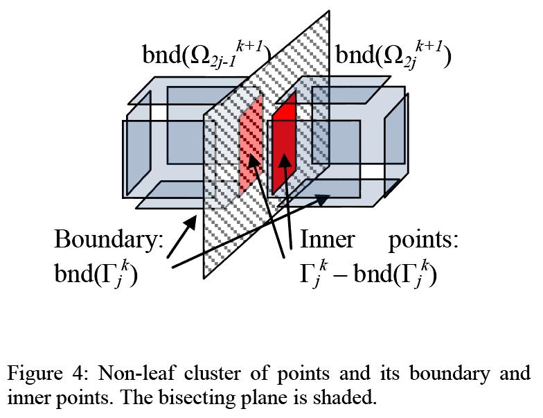
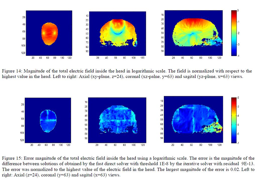
88 Accelerated nested dissection on grids in R 3 We have implemented the accelerated nested dissection method to solve the electrostatics problems arising in transcranial magnetic stimulation (TMS). This environment is characterized by: There is time to preprocess a given geometry. Given a load, the solution should be found instantaneously. Joint work with Frantisek Cajko, Luis Gomez, Eric Michielssen, and, Luis Hernandez-Garcia of U. Michigan.

89

90 Numerical results: Single CPU desktop. Local accuracy was 1. Our benchmark was the Pardiso package in Intel s MKL. N Storage (MB) Factorization (sec) Solution (sec) Pardiso FDS Pardiso FDS Pardiso FDS 32 3 = = = = = Note: Direct solvers require substantially more memory than, e.g., multigrid. Note: The gain over Pardiso is modest for small problem sizes, but: FDS has better asymptotic scaling as N grows. FDS is better suited for large-scale parallelization. FDS will be extremely fast for pure boundary value problems (this is speculation... ) The FDS methods are still fairly immature; improvements are to be expected.

91

92 There may be short-cuts to finding the inverses... Recent work indicates that randomized sampling could be used to very rapidly find a data-sparse representation of a matrix (in H / H 2 / HSS /... format). The idea is to extract information by applying the operator to be compressed to a sequence of random vectors. In the present context, applying the inverse of course corresponds simply to a linear solve. Fast construction of hierarchical matrix representation from matrix-vector multiplication, L. Lin, J. Lu, L. Ying., J. of Computational Physics, 23(1), 211. P.G. Martinsson, A fast randomized algorithm for computing a Hierarchically Semi-Separable representation of a matrix. SIAM J. on Matrix Analysis and Appl., 32(4), pp , 211. For more on randomized sampling in numerical linear algebra, see: N. Halko, P.G. Martinsson, J. Tropp, Finding structure with randomness: Probabilistic algorithms for constructing approximate matrix decompositions. SIAM Review, 53(2), 211. pp

93 Question: When are the boundary operators compressible in HSS form? Electrostatics on a network of resistors. The object computed is the lattice Neumannto-Dirichlet boundary operator. It maps a vector of fluxes on the blue nodes to a vector of potentials on the blue nodes. Question: How compressible is the N2D operator? Case A: Constant conductivities standard 4/-1/-1/-1/-1 five-point stencil. Case B: Random conductivities drawn uniformly from the interval [1, 2]. Case C: Periodic oscillations high aspect ratio. Case D: Random cuts 5% of the bars were cut, the others have unit conductivity. Case E: Large cracks.

94 Case C periodic oscillations: x 2 x x x Conductivities Typical solution field

95 Case E large cracks: Sink Source x x Geometry Permissible solution field

96 Memory requirements in floats per degree of freedom: All operators were compressed to a relative accuracy of 1 1. N side N side N side N side N side = 1 = 2 = 4 = = 16 General matrix Case A (constant conductivities) Case B (periodic conductivities) Case C (random conductivities) Case D (random cuts) Case E (cracks) Key observations: The amount of memory required is essentially problem independent. Almost perfect linear scaling.

97 A conduction problem on a perforated domain Geometry Potential The Neumann-to-Dirichlet operator for the exterior boundary was computed. The boundary was split into 44 panels, with 26 Gaussian quadrature nodes on each one. This gives a relative accuracy of 1 1 for evaluating fields at points very close to the boundary (up to.5% of the side-length removed). Storing the N2D operator (in a data-sparse format) requires 12 floats per degree of freedom.

98 A conduction problem on a perforated domain close to percolation Geometry Potential The Neumann-to-Dirichlet operator for the exterior boundary was computed. The boundary was split into 44 panels, with 26 Gaussian quadrature nodes on each one. This gives a relative accuracy of 1 1 for evaluating fields at points very close to the boundary (up to.5% of the side-length removed). Storing the N2D operator (in a data-sparse format) requires 11 floats per degree of freedom.

99 Question: When are the boundary operators compressible in HSS form? Apparent answer: Almost always for non-oscillatory problems. (?) Dense matrices that arise in numerical algorithms for elliptic PDEs are surprisingly well suited to the HSS-representation. The format is robust to: Irregular grids. PDEs with non-smooth variable coefficients. Inversion, LU-factorization, matrix-matrix-multiplies, etc. For oscillatory problems, the ranks grow as the wave-length of the problem is shrunk relative to the size of the geometry, which eventually renders the direct solvers prohibitively expensive. However, the methodology remains efficient for surprisingly small wave-lengths. Some supporting theory and intuitive arguments exist, but the observed performance still exceeds what one would expect, both in terms of the range of applicability and what the actual ranks should be. (At least what I would expect!)

100 Assertions: Fast direct solvers excel for problems on 1D domains. (They should become the default.) Integral operators on the line. Boundary Integral Equations in R 2. Boundary Integral Equations on rotationally symmetric surfaces in R 3. Existing fast direct solvers for finite element matrices associated with elliptic PDEs in R 2 work very well. In R 3, they can be game-changing in specialized environments. Predictions: For BIEs associated with non-oscillatory problems on surfaces in R 3, the complexity will be reduced from O(N(log N) p ) to O(N), with a modest scaling constant. Randomized methods will prove enormously helpful. They have already demonstrated their worth in large scale linear algebra. Direct solvers for scattering problems will find users, even if expensive. O(N 1.5 ) or O(N 2 ) flop counts may be OK, provided parallelization is possible. Direct solvers will provide a fantastic tool for numerical homogenization. Open questions: How efficient can direct solvers be for volume problems in 3D? Are O(N) direct solvers for highly oscillatory problems possible?