Section 7.2 Euler s Method

Transcription

1 Section 7.2 Euler s Method Key terms Scalar first order IVP (one step method) Euler s Method Derivation Error analysis Computational procedure Difference equation Slope field or Direction field Error

2 Euler's method is the simplest of the one-step methods for approximating the solution to the initial value problem. An outline of the general procedure follows. A scalar, first-order initial value problem is given as We want to determine a numerical approximation to y(t) at discrete points in the interval [a, b]. The true solution of the IVP is denoted y(t) and we adopt the notational convention that w i represents the approximation to y i = y(t i ). (Note that y i is a short hand notation for the value of the true solution at t i.) For simplicity, the approximate solution will be sought at equally spaced points; that is, for some positive integer N, we will define the step size h = (b a)/n and t i will be given by t i = a + ih, (I = 0, 1, 2,, N). For a number of techniques we develop the step size will be constant; i.e. equispaced points.

3 Derivation of Euler s Method The derivation is another application of Taylor series. Assume that the true solution y(t) of the IVP has two continuous derivatives. Expanding this true solution in a Taylor series about the point t = t i produces where ξ is guaranteed to lie between t and t i. Evaluating the above Taylor expansion at t = t i+1 and substituting for y i ꞌ from the right-hand side of the differential equation, we obtain the next estimate Euler's method arises by dropping the error term and replacing y i (exact solution) by w i (approximate solution):

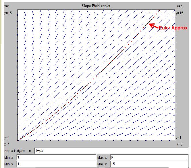
4 Example: Approximate IVP For this problem, f(t, x) is given by f(t, x) = 1 + x/t, so that the Euler's method difference equation takes the form Let's use a step size of h = 0.5, which will require ten steps to advance from t = 1 to t = 6. With t 0 = 1 and w 0 = 1, we calculate Advancing the value of the independent variable from t 0 to t 1 = t 0 + h = 1.5, we then calculate ETC. The exact solution is x(t) = t(1 + ln t). Thus we shall compare the Euler approximation and the exact solution.

5 Error Inspect the scales for the graphs. Approximate (solid) + True Soln (dotted) ABS. ERROR

6

7 Observe the slow but steady growth in the global error as t increases. Since each step introduces new error into the computed approximate solution, we might expect this type of behavior in every problem; however, the actual accumulation of global error is very problem dependent.

8 Essentially, the error introduced by each step of the time marching process moves us from one solution of the differential equation onto a different solution. (At each step we encounter a new IVP; a perturbed IVP.) If, nearby solutions separate from one another as t increases, we can expect to see a steady increase in the global error. Note that a change of initial conditions had those solution curves move away from the solution curve for the original IVP. On the other hand, if nearby solutions move closer together as t increases, we could expect to observe a steady decline in the global error. The next example demonstrates this situation.

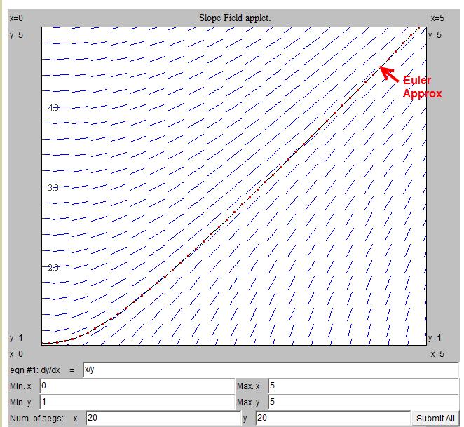
9 Another Example: IVP Here the Euler's method difference equation takes the form The exact solution is Here nearby solutions move closer together as t increases, so we observe a steady decline in the global error.

10 Approximate (solid) + True Soln (dotted) ABS. ERROR

11

12 In this case changes in the initial conditions have the nearby solutions move closer together as t increases. So we could expect to observe a steady decline in the global error.

13 Next we need to determine the rate of convergence of Euler s method as the stepsize h decreases; h 0. Let's perform a numerical experiment. We expect that the accuracy of the approximate solution generated by Euler's method will improve if we decrease the step size h, but how much improvement will we obtain? Is the global error O(h)? Is it O(h 2 )? Is it O(h 3 )? The idea is that for each of our two examples we investigate the approximation at the end of solution interval for decreasing step sizes h. We halve the stepsize and look at how the error changes. Approx at t = 6. Note each time the step size is cut by a factor of 2, the absolute error shrinks by roughly the same factor. This suggests that the global error associated with Euler's method is O(h).

14 Approx at t = 5 Once again, each time the step size is cut by a factor of 2, the absolute error shrinks by roughly the same factor. So we conjecture that the rate of convergence of Euler s method is O(h).

15 Analysis of Euler s Method Euler s method is the simplest one-step method for approximating the solution of an IVP. Even so analyzing the error in Euler s method is not easy. We will outline the results. We start with the local truncation error which is

16 Basically this says, that if we choose h small enough we may get reasonable results. But we still need to see how the global error behaves. Here is where things get mathematically messy. We need the following condition: it is a vertical growth condition within a set D in the domain. Definition: A function f(t, y) satisfies a Lipschitz Condition in y on a set D in R 2 if there exists a constant L > 0 such that f(t, y 1) f(t, y 2 ) L y1 y2 For all ordered pairs (t, y 1 ) and (t, y 2 ) in set D. The constant L is called the Lipschitz Constant. A given function may satisfy a Lipschitz condition on one set, but not on another. Also, value of L may depend on the set D.

17 The next theorem deals with the accumulated error since w i depends on the previous approximations, w i-1, w i-2,, w 1. (We state this without a proof which requires some results involving sequences.) Note y i w i is the accumulated error in approximation w i at t = t i, assuming all the arithmetic was done exactly.

18

19 Global error at t = t i.

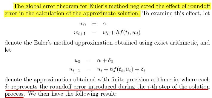
20 When the effect of roundoff is included the global error is composed of two competing forces. Finally if f(t,y) satisfies a Lipschitz condition in y, then it can be shown that Euler s method is stable with respect to perturbations of the initial conditions.

21 The truncation error in Euler's method can be reduced by using a smaller step size h; the reduction in error being linear with h. As the value of h is reduced, the number of steps to be used increases, thereby, increasing the round-off error. Thus, the round-off error increases as the truncation error decreases, as shown qualitatively in the figure. Although this figure shows that there is an optimum step size to minimize the total error, usually its value is not known. Hence, in practice, for a given differential equation, a series of solutions, each with a smaller step size, can be generated until two successive step sizes give essentially the same solution. At that stage, the solution can be assumed to have converged to the exact solution. However, it is to be noted that, due to the presence of round-off error, the numerical solution will always be different from the exact solution. In the absence of round-off errors, if a numerical solution approaches the exact solution as the step size (h) approaches zero, the numerical method is said to be convergent.