NOTES FOR 18.04, Spring 2017

Transcription

1 NOTES FOR 8.04, Spring course introduction 0. Brief course description Jeremy Orloff omplex analysis is a beautiful, tightly integrated subject. It revolves around complex analytic functions. These are functions that have a complex derivative. Unlike calculus using real variables, the mere existence of a complex derivative has strong implications for the properties of the function. There are a small number of far-reaching theorems that we ll explore in the first part of the class. Along the way, we ll touch on some mathematical and engineering applications of these theorems. The last third of the class will be devoted to a deeper look at applications. The main theorems are auchy s Theorem, auchy s integral formula, and the existence of Taylor and Laurent series. Among the applications will be harmonic functions, two dimensional fluid flow, easy methods for computing (seemingly) hard integrals, Laplace transforms, and Fourier transforms with applications to engineering and physics. 0.2 Topics needed from prerequisite math classes We will review these topics as we need them: Limits Power series Vector fields Line integrals Green s theorem 0.3 Level of mathematical rigor We will make careful arguments to justify our results. Though, in many places we will allow ourselves to skip some technical details if they get in the way of understanding the main point, but we will note what was left out. omplex algebra and the complex plane We will start with a review of the basic algebra and geometry of complex numbers. Most likely you have encountered this previously in 8.03 or elsewhere.

2 OMPLEX ALGEBRA AND THE OMPLEX PLANE 2. Motivation The equation x 2 = has no real solutions, yet we know that this equation arises naturally and we want to use its roots. So we make up a new symbol for the roots and call it a complex number. Definition. The symbols ±i will stand for the solutions to the equation x 2 =. We will call these new numbers complex numbers. We will also write = ±i Notes:. i is also called an imaginary number. This is a historical term. These are perfectly valid numbers that don t happen to lie on the real number line. 2. Our motivation for using complex numbers is not the same as the historical motivation. Historically, mathematicians were willing to say x 2 = had no solutions. The issue that pushed them to accept complex numbers had to do with the formula for the roots of cubics. ubics always have at least one real root, and when square roots of negative numbers appeared in this formula, even for the real roots, mathematicians were forced to take a closer look at these (seemingly) exotic objects. We re going to look at the algebra, geometry and, most important for us, the exponentiation of complex numbers. Before starting a systematic exposition of complex numbers, we ll work a simple example. Example.. Solve the equation z 2 + z + = 0. answer: We can apply the quadratic formula to get z = ± 4 2 = ± 3 2 = ± 3 2. = ± 3 i. 2 Think: Do you know how to solve quadratic equations by completing the square? This is how the quadratic formula is derived and is well worth knowing!.. Fundamental theorem of algebra One of the reasons for using complex numbers is because allowing complex roots means every polynomial has exactly the expected number of roots. This is the fundamental theorem of algebra: Fundamental theorem of algebra. A polynomial of degree n has exactly n complex roots (repeated roots are counted with multiplicity). In a few weeks, we will be able to prove this theorem as a remarkably simple consequence of one of our main theorems..2 Terminology and basic arithemetic Definitions.

3 OMPLEX ALGEBRA AND THE OMPLEX PLANE 3 omplex numbers are defined as the set of all numbers where x and y are real numbers. z = x + yi, We denote the set of all complex numbers by. (On the blackboard we will usually write this font is called blackboard bold.) We call x the real part of z. This is denoted by x = Re(z). We call y the imaginary part of z. This is denoted by y = Im(z). Note well: The imaginary part of z is a real number. It DOES NOT include the i. Note. Engineers typically use j instead of i. We ll follow mathematical custom in The basic arithmetic operations follow the standard rules. All you have to remember is that i 2 =. We will go through these quickly using some simple examples. It almost goes without saying that in 8.04 it is essential that you become fluent with these manipulations. Addition: (3 + 4i) + (7 + i) = 0 + 5i Subtraction: (3 + 4i) (7 + i) = 4 7i Multiplication: (3 + 4i)(7 + i) = i + 33i + 44i 2 = i. Here we have used the fact that 44i 2 = 44. Before talking about division and absolute value we introduce a new operation called conjugation. It will prove useful to have a name and symbol for this, since we will use it frequently. omplex conjugation is denoted with a bar and defined by x + iy = x iy. If z = x + iy then its conjugate is z = x iy and we read this as z-bar = x iy. Example i = 3 5i. The following is a very useful property of conjugation. We will use it in the next example to help with division. Useful property of conjugation: If z = x + iy then zz = (x + iy)(x iy) = x 2 + y 2 (is real). Example.3. (Division.) Write 3 + 4i in the standard form x + iy. + 2i answer: We use the useful property of conjugation to clear the denominator: 3 + 4i + 2i = 3 + 4i + 2i 2i 2i = = 2i i. In the next section we will discuss the geometry of complex numbers, which give some insight into the meaning of the magnitude of a complex number. For now we just give the definition.

4 OMPLEX ALGEBRA AND THE OMPLEX PLANE 4 Definition. The magnitude of the complex number x + iy is defined as z = x 2 + y 2. The magnitude is also called the absolute value, norm or modulus. Example.4. The norm of 3 + 5i = = 34. Note this really well. The norm is the sum of x 2 and y 2 it does not include the i! Therefore it is always positive..3 The complex plane and the geometry of complex numbers Because it takes two numbers x and y to describe the complex number z = x + iy we can visualize complex numbers as points in the xy-plane. When we do this we call it the complex plane. Since x is the real part of z we call the x-axis the real axis. Likewise, the y-axis is the imaginary axis. Imaginary axis θ r x z = x + iy = (x, y) y Real axis Imaginary axis r θ θ r z = x + iy = (x, y) Real axis z = x iy = (x, y).4 Polar coordinates In the figures above we have marked the length r and polar angle θ of the vector from the origin to the point z = x + iy. These are the same polar coordinates you saw in 8.02 and There are a number of synonyms for both r and θ r = z = magnitude = length = norm = absolute value = modulus θ = arg(z) = argument of z = polar angle of z As in 8.02 you should be able to visualize polar coordinates by thinking about the distance r from the origin and the angle θ with the x-axis. Example.5. In this example we make a table of z, r and θ for some complex numbers. Notice that θ is not uniquely defined since we can always add a multiple of 2π to θ and still be at the same point in the plane. z = a + bi r θ 0, 2π, 4π,... Argument = 0, means z is along the x-axis i π/2, π/2 + 2π... Argument = π/2, means z is along the y-axis + i 2 π/4, π/4 + 2π... Argument = π/4, means z is along the ray at 45 to the x-axis

5 OMPLEX ALGEBRA AND THE OMPLEX PLANE 5 Imaginary axis i + i Real axis When we want to be clear which value of θ is meant, we will specify a branch of arg. For example, 0 θ < 2π or π < θ π. This will be discussed in much more detail in the coming weeks. Keeping careful track of the branches of arg will turn out to be one of the key requirements of complex analysis..5 Euler s Formula Euler s (pronounced oilers ) formula connects complex exponentials, polar coordinates, and sines and cosines. It turns messy trig identities into tidy rules for exponentials. We will use it a lot. The formula is the following: e iθ = cos(θ) + i sin(θ). () There are many ways to approach Euler s formula. Our approach is to simply take Equation as the definition of complex exponentials. This is legal, but does not show that it s a good definition. To do that we need to show the e iθ obeys all the rules we expect of an exponential. To do that we go systematically through the properties of exponentials and check that they hold for complex exponentials..5. e iθ behaves like a true exponential. e it differentiates as expected: deit dt = ie it. Proof. This follows directly from the definition: de it dt = d dt (cos(t) + i sin(t)) = sin(t) + i cos(t) = i(cos(t) + i sin(t)) = ieit. QED 2. e i 0 =. Proof. e i 0 = cos(0) + i sin(0) =. QED 3. The usual rules of exponents hold: e ia e ib = e i(a+b). Proof. This relies on the cosine and sine addition formulas. e ia e ib = cos(a) + i sin(b) (cos(a) + i sin(b)) = cos(a) cos(b) sin(a) sin(b)) + i (cos(a) sin(b) + sin(a) cos(b)) = cos(a + b) + i sin(a + b) = e i(a+b).

6 OMPLEX ALGEBRA AND THE OMPLEX PLANE 6 4. The definition of e iθ is consistent with the power series for e x. Proof. To see this we have to recall the power series for e x, cos(x) and sin(x). They are e x = + x + x 2 /2! + x 3 /3! + x 4 /4! +... cos(x) = x 2 /2! + x 4 /4 x 6 /6! +... sin(x) = x x 3 /3! + x 5 /5! +... Now we can write the power series for e iθ and then split it into the power series for sine and cosine: e iθ (iθ) n = n! 0 = ( ) k θ2k (2k)! + i ( ) k θ 2k+ (2k + )! 0 = cos(θ) + i sin(θ). So the Euler formula definition is consistent with the usual power series for e z. -4 should convince you that e iθ behaves like an exponential ompex exponentials and polar form Now let s turn to the relation between polar coordinates and complex exponentials. Suppose z = x + iy has polar coordinates r and θ. That is, we have x = r cos(θ) and y = r sin(θ). Thus, we get the important relationship z = x + iy = r cos(θ) + ir sin(θ) = r(cos(θ) + i sin(θ)) = re iθ. This is so important you shouldn t proceed without understanding. without the intermediate equation. We also record it z = x + iy = re iθ. (2) Because r and θ are the polar coordinates of (x, y) we call z = re iθ the polar form of z. Magnitude, argument, conjugate, multiplication and division are easy in polar form. Magnitude. e iθ =. Proof. e iθ = cos(θ) + i sin(θ) = cos 2 (θ) + sin 2 (θ) =. In words, this says that e iθ is always on the unit circle this is useful to remember! Likewise, if z = re iθ then z = r. You can calculate this, but it should be clear from the definitions: z is the distance from z to the origin, which is exactly the same definition as for r. Argument. If z = re iθ then arg(z) = θ. Proof. This is again the definition: the argument is the polar angle θ. onjugate. (re iθ ) = re iθ. Proof. (re iθ ) = (r(cos(θ) + i sin(θ))) = r(cos(θ) i sin(θ)) = re iθ.

7 OMPLEX ALGEBRA AND THE OMPLEX PLANE 7 In words: complex conjugation changes the sign of the argument. Multiplication. If z = r e iθ and z 2 = r 2 e iθ 2 then z z 2 = r r 2 e i(θ +θ 2 ). This is what mathematicians call trivial to see, just write the multiplication down. In words, the formula says the for z z 2 the magnitudes multiply and the arguments add. Division. Again it s trivial that r e iθ r 2 e iθ 2 = r r e i(θ θ 2 ). Example.6. Multiplication by 2i. Here s a simple but important example. By looking at the graph we see that the number 2i has magnitude 2 and argument π/2. So in polar coordinates it equals 2e iπ/2. This means that multiplication by 2i multiplies lengths by 2 and adds π/2 to arguments, i.e. rotates by 90. The effect is shown in the figures below Im Im 2i Im 2i = 2e iπ/2 π/2 Re Re Re 2i = 2, arg(2i) = π/2 Multiplication by 2i rotates by π/2 and scales by 2 Example.7. Raising to a power. ompute (i) ( + i) 6 ; (ii) ( ) 3 +i 3 2 answer: (i) + i has magnitude = 2 and arg = π/4, so + i = 2e iπ/4. Raising to a power is now easy: (ii) + i 3 2 = e iπ/3, so ( + i) 6 = ( 2e iπ/4 ) 6 = 8e 6iπ/4 = 8e 3iπ/2 = 8i. ( + i ) 3 3 = ( e iπ/3 ) 3 = e iπ = 2 Example.8. omplexification or complex replacement. In this example we illustrate the technique of complex replacement to simplify a trigonometric integral. This technique will come in handy when we need to compute certain integrals. Problem. ompute I = e x cos(2x) dx. answer: We have Euler s formula e 2ix = cos(2x) + i sin(2x), so cos(2x) = Re(e 2ix ). The complex replacement trick is to replace cos(2x) by e 2ix. We get (justification below) I c = e x cos 2x + ie x sin 2x dx, I = Re(I c ). omputing I c is straightforward: I c = e x e i2x dx = e x(+2i) dx = ex(+2i) + 2i.

8 OMPLEX ALGEBRA AND THE OMPLEX PLANE 8 Using rectangular coordinates. Here we will do the computation in rectangular coordinates. In applictations, for example throughout 8.03, polar form is preferred because it is easier and gives the answer in a more useable form. I c = ex(+2i) + 2i 2i 2i = ex (cos(2x) + i sin(2x))( 2i) 5 = 5 ex (cos(2x) + 2 sin(2x) + i( 2 cos(2x) + sin(2x))) So, I = Re(I c ) = 5 ex (cos(2x) + 2 sin(2x)). Justification of complex replacement. The trick comes by cleverly adding a new integral to I as follows. Let J = e x sin(2x) dx. Then we let I c = I + ij = e x (cos(2x) + i sin(2x)) dx = e x e 2ix dx. learly, by construction, Re(I c ) = I as claimed above. Alternative using polar coordinates to simplify the expression for I c : Write + 2i = re iφ, where r = 5 and φ = arg( + 2i) = tan (2) in the first quadrant. Then: I c = ex(+2i) 5e iφ Thus, I = Re(I c ) = ex 5 cos(2x φ). = ex 5 e i(2x φ) = ex 5 (cos(2x φ) + i sin(2x φ))..5.3 Nth roots We are going to need to be able to find the nth roots of complex numbers. The trick is to recall that a complex number has more than one argument, that is we can always add a multiple of 2π. For example, Example.9. Find all 5 fifth roots of 2. 2 = 2e 0i = 2e 2πi = 2e 4πi... = 2e 2nπi answer: In polar form: ( 2e 2nπi) /5 = 2 /5 e 2nπi/5. So the fifth roots of 2 are 2 /5 = 2 /5 e 2nπi/5, where n = 0,, 2,... The notation is a little strange, because the 2 /5 on the left side of the equation means the complex roots and the 2 /5 on the right hand side is a magnitude, so it is the positive real root. Looking at the left hand side we see that for n = 5 we have 2 /5 e 2πi which is exactly the same as the root when n = 0, i.e. 2 /5 e 0i. Likewise n = 6 gives exactly the same root as n =. So, we have 5 different roots corresponding to n = 0,, 2, 3, 4. 2 /5 = 2 /5, 2 /5 e 2πi/5, 2 /5 e 4πi/5, 2 /5 e 6πi/5, 2 /5 e 8πi/5.

9 OMPLEX ALGEBRA AND THE OMPLEX PLANE 9 Similarly we can say that in general z = re iθ has N different Nth roots: z /N = r /N e iθ/n+i 2π(n/N) for 0,, 2,... N. Example.0. Find the 4 fourth roots of. answer: = e i 2πn, so /4 = e i 2π(n/4). So the 4 different fourth roots are, e i π/2, e i π, e i 3π/2, e i 2π. When the angles are ones we know about, e.g. 30, 60, 90, 45, etc., we should simplify the complex exponentials. In this case, the roots are, i,, i. Example.. Find the 3 cube roots of -. answer: = e i π+i 2πn. So, ( ) /3 = e i π/3+i 2π(n/3) and the 3 cube roots are e iπ/3, e iπ, e i5π/3. Since π/3 radians is 60 we can simpify: e iπ/3 = cos(π/3) + i sin(π/3) = i ( ) /3 =, ± 2. Example.2. Find the 5 fifth roots of + i. answer: + i = 2e i(π/4+2nπ), for n = 0,, 2,.... So, the 5 fifth roots are ( + i) /5 = 2 /0 e iπ/20, 2 /0 e i9π/20, 2 /0 e i7π/20, 2 /0 e i25π/20, 2 /0 e i33π/20. Using a calculator we could write these numerically as a + bi, but there is no easy simplification. Example.3. We should check that our technique works as expected for a simple problem. Find the 2 square roots of 4. answer: 4 = 4e i 2πn. So, 4 /2 = 2e i πn. So the 2 square roots are = 2e 0, 2e iπ = ±2 as expected!.5.4 The geometry of nth roots Looking at the examples above we see that roots are always spaced evenly around a circle centered at the origin. For example, the fifth roots of + i are spaced at increments of 2π/5 radians around the circle of radius 2 /5. Note also that the roots of real numbers always come in conjugate pairs. y y 2 + i i x x ube roots of - 2 i 3 2 Fifth roots of + i.6 Inverse Euler Formula Euler s formula gives a complex exponential in terms of sines and cosines. We can turn this around to get the inverse Euler formulas.

10 OMPLEX ALGEBRA AND THE OMPLEX PLANE 0 Euler s formula says: By adding and subtracting we get: e it = cos(t) + i sin(t) and e it = cos(t) i sin(t). cos(t) = eit + e it 2 and sin(t) = eit e it. 2i Please take note of these formulas we will use them frequently!.7 Representing complex multiplication as matrix multiplication onsider the product w = (a + bi)(x + iy) = (ax by) + i(bx + ay) We can think of points in the complex plane z = x + iy as two-dimensional vectors in R 2, e.g. [ ] [ ] x ax by z = x + iy, w = (ax by) + i(bx + ay) y bx + ay It s easy to see that as vectors we have [ ] [ ] [ ] ax by a b x = bx + ay b a y [ That is, ] in this sense, multiplication by a + ib is the same as multiplication by the matrix a b. We will not make a lot of use of this fact, but later it will help us remember b a certain formulas and facts. [ ] 0 Example.4. Multiplication by i is represented by the matrix. 0.8 de Moivre s formula de Moivre s formula: For positive integers n: (cos(θ) + i sin(θ)) n = cos(nθ) + i sin(nθ) Proof. This is a simple consequence of Euler s formula: (cos(θ) + i sin(θ)) n = (e iθ ) n = e inθ = cos(nθ) + i sin(nθ) QED The reason this simple fact has a name is that historically de Moivre stated it before Euler s formula was known. Without Euler s formula there is not such a simple proof.

11 OMPLEX ALGEBRA AND THE OMPLEX PLANE.9 The exponential function We have Euler s formula: e iθ = cos(θ) + i sin(θ). We can extend this to the complex exponential function e z. Definition. For z = x + iy the complex exponential function is defined as e z = e x+iy = e x e iy = e x (cos(y) + i sin(y)). In this definition e x is the usual exponential function for a real variable x. It is easy to see that all the usual rules of exponents hold:. e 0 = 2. e z +z 2 = e z e z 2 3. (e z ) n = e nz for positive integers z. 4. (e z ) = e z 5. e z 0 It will turn out that the property dez dz = ez also holds, but we can t prove this yet because we haven t defined what we mean by the complex derivative d dz. Here are some more simple, but extremely important properties of e z. You should become fluent in their use and know how to prove them. 6. e iθ = Proof. e iθ = cos(θ) + i sin(θ) = cos 2 (θ) + sin 2 (θ) =. 7. e x+iy = e x (as usual z = x + iy and x, y are real). Proof. You should be able to supply this. If not: ask a teacher or TA. 8. The path e it for 0 < t < wraps counterclockwise around the unit circle. It does so infinitely many times. This is illustrated in the following picture. z = e it e πi/2 = e 5πi/2 3e πi/4 = e πi/4 e πi/4 = e 9πi/4 0 π 4 π 2 3π 4 π 5π 4 3π 2 7π 4 2π 9π 4 5π 2 π 4 3π 3π 4 7π 2 5π 4 4π t e πi = e 3πi e 0 = e 2πi = e 4πi 5e πi/4 = e 3πi/4 7e πi/4 = e 5πi/4 The map t e it wraps around the unit circle. e 3πi/2 = e 7πi/2

12 OMPLEX ALGEBRA AND THE OMPLEX PLANE 2.0 omplex functions as mappings A complex function w = f(z) is hard to graph because it takes 4 dimensions: 2 for z and 2 for w. So, to visualize them we will think of complex functions as mappings. That is we will think of w = f(z) as taking a number in the complex z-plane and mapping (sending) it to a number in the complex w-plane. We will use the following terms and symbols to discuss mappings. A function w = f(z) will also be called a mapping of z to w. Alternatively we will write z w or z f(z). This is read as z maps to w. We will say that w is the image of z under the mapping or more simply w is the image of z. If we have a set of points in the z-plane we will talk of the image of that set under the mapping. For example, under the mapping z iz the image of the imaginary z-axis is the real w-axis. Im(z) z w = iz Im(w) i Re(z) Re(w) The image of the imaginary axis under z iz. Now we ll illustrate visualizing mappings with some examples: Example.5. The mapping w = z 2. We visualize this by putting the z-plane on the left and the w-plane on the right. We then draw various curves and regions in the z-plane and the corresponding image under z 2 in the w-plane. In the first figure we show that rays from the origin are mapped by z 2 to rays from the origin. We see that. The ray L 2 at π/4 radians is mapped to the ray f(l 2 ) at π/2 radians. 2. The rays L 2 and L 6 are both mapped to the same ray. This is true for each pair of diametrically opposed rays. 3. A ray at angle θ is mapped to the ray at angle 2θ.

13 OMPLEX ALGEBRA AND THE OMPLEX PLANE 3 Im(z) z w = z 2 L4 L3 L2 f(l2) & f(l6) L5 L Re(z) f(l3) & f(l7) f(l) & f(l5) L6 L7 L8 f(l4) & f(l8) f(z) = z 2 maps rays from the origin to rays from the origin. The next figure gives another view of the mapping. Here we see vertical stripes in the first quadrant are mapped to parabolic stripes that live in the first and second quadrants. Im(w) z w = z Im(z) Re(z) Re(w) z 2 = (x 2 y 2 ) + i2xy maps vertical lines to left facing parabolas. The next figure is similar to the previous one, except in this figure we look at vertical stripes in both the first and second quadrants. We see that they map to parabolic stripes that live in all four quadrants.

14 OMPLEX ALGEBRA AND THE OMPLEX PLANE 4 Im(w) z w = z Im(z) Re(z) Re(w) f(z) = z 2 maps the first two quadrants to the entire plane. The next figure shows the mapping of stripes in the first and fourth quadrants. The image map is identical to the previous figure. This is because the fourth quadrant is minus the second quadrant, but z 2 = ( z) 2. Im(w) z w = z Im(z) Re(z) Re(w) Vertical stripes in quadrant 4 are mapped identically to vertical stripes in quadrant 2.

15 OMPLEX ALGEBRA AND THE OMPLEX PLANE 5 z w = z 2 Im(z) Im(w) Re(z) Re(w) Simplified view of the first quadrant being mapped to the first two quadrants. z w = z 2 Im(z) Im(z) Re(z) Re(z) Simplified view of the first two quadrants being mapped to the entire plane. Example.6. The mapping w = e z. Here we present a series of plots showing how the exponential function maps z to w. Im(z) Im(w) 2πi + 2πi z w = e z e e 2 Re(w) πi/2 + πi/2 0 2 Re(z) Notice that vertical lines are mapped to circles and horizontal lines to rays from the origin. The next four figures all show essentially the same thing: the exponential function maps horizontal stripes to circular sectors. Any horizontal stripe of width 2π gets mapped to the entire plane minus the origin, Because the plane minus the origin comes up frequently we give it a name: Definition. The punctured plane is the complex plane minus the origin. In symbols we can write it as {0} or /{0}.

16 OMPLEX ALGEBRA AND THE OMPLEX PLANE 6 Im(z) 2πi z w = e z Im(w) πi πi/2 e e 2 Re(w) 0 2 Re(z) πi The horizontal 0 y < 2π is mapped to the punctured plane Im(z) 2πi z w = e z Im(w) πi πi/2 e e 2 Re(w) 0 2 Re(z) πi The horizontal π < y π is mapped to the punctured plane Im(z) 2πi z w = e z Im(w) πi Re(w) 0 Re(z) Simplified view showing e z maps the horizontal stripe 0 y < 2π to the punctured plane.

17 OMPLEX ALGEBRA AND THE OMPLEX PLANE 7 z w = e z Im(w) Im(z) πi 0 Re(z) Re(w) πi Simplified view showing e z maps the horizontal stripe π < y π to the punctured plane.. log(z) and arg(z).. Many-to-one functions The function f(z) = z 2 maps ±z to the same value, e.g. f(2) = f( 2) = 4. We say that f(z) is a 2-to- function. That is, it maps 2 different points to each value. (Technically, it only maps one point to 0, but we will gloss over that for now.) Here are some other examples of many-to-one functions. Example.7. w = z 3 is a 3-to- function. For example, 3 different z values get mapped to w = : ( 3 + ) 3 ( 3 i ) 3 3 i = = = 2 2 Example.8. The function w = e z maps infinitely many points to each value. For example e 0 = e 2πi = e 4πi =... e 2nπi =... = e iπ/2 = e iπ/2+2πi = e iπ/2+4πi =... e iπ/2+2nπi =... = i In general, e z+2nπi has the same value for every integer n...2 Branches of arg(z) Important note. You should master this section. Branches of arg(z) are the key that really underlies all our other examples. Fortunately it is reasonably straightforward. The key point is that the argument is only defined up to multiples of 2πi so every z produces infinitely many values for arg(z). Because of this we will say that arg(z) is a multiple-valued function. Note. You might complain that by definition a function must take just one value. And you would be right. But we will call functions like arg(z) or z (which has 2 possible values) multiple-valued. What that means in practice is that whenever we use such a function

18 OMPLEX ALGEBRA AND THE OMPLEX PLANE 8 will have to be careful to specify which of the possible values we mean. This is known as specifying a branch of the function. Definition. By a branch of the argument function we mean any interval of length 2π. By specifying a branch we are saying that we will take the single value of arg(z) that lies in the branch. Let s look at several different branches to understand how they work: (i) If we specify the branch as 0 arg(z) < 2π then we have the following arguments. arg() = 0; arg(i) = π/2; arg( ) = π; arg( i) = 3π/2 This branch and these points are shown graphically in Figure (i) below. arg = π/2 arg = 3π/4 arg = π/4 arg = π arg π arg = 0 arg 2π arg = 5π/4 arg = 7π/4 arg = 3π/2 Figure (i): The branch 0 arg(z) < 2π of arg(z). Notice that if we start at z = on the positive real axis we have arg(z) = 0. Then arg(z) increases as we move counterclockwise around the circle. The argument is continuous until we get back to the positive real axis. There it jumps from almost 2π back to 0. There is no getting around (no pun intended) this discontinuity. We will call the line where the discontinuity happens the branch cut for this branch of arg(z). It is shown as a thick orange line in the figure. For future reference you should note that near the negative real axis arg(z) is continuous and the arguments of nearby points are close to each other. (ii) If we specify the branch as π < arg(z) π then we have the following arguments: arg() = 0; arg(i) = π/2; arg( ) = π; arg( i) = π/2 This branch and these points are shown graphically in Figure (ii) below.

19 OMPLEX ALGEBRA AND THE OMPLEX PLANE 9 arg = π/2 arg = 3π/4 arg = π/4 arg = π arg π arg = 0 arg 0 arg = 3π/4 arg = π/4 arg = π/2 Figure (ii): The branch π < arg(z) π of arg(z). ompare this figure with Figure (i). The values of arg(z) are the same in the upper half plane, but in the lower half plane they differ by 2π. For this branch the branch cut is along the negative real axis. As we cross the branch cut the value of arg(z) jumps from π to something close to π. (iii) Figure (iii) shows the branch of arg(z) with π/4 arg(z) < 9π/4. arg = π/2 arg = 3π/4 arg = π/4 arg 9π/4 arg = π arg π arg = 2π arg 2π arg = 5π/4 arg = 7π/4 arg = 3π/2 Figure (iii): The branch π/4 arg(z) < 9π/4 of arg(z). Notice that on this branch arg(z) is continuous at both the positive and negative real axes. The jump of 2π occurs along the ray at angle π/4. (iv) Obviously, there are many many possible branches. For example, 42 < arg(z) π. (v) We won t make use of this in 8.04, but, in fact, the branch cut doesn t have to be a

20 OMPLEX ALGEBRA AND THE OMPLEX PLANE 20 straight line. Any curve that goes from the origin to infinity will do. The argument will be continuous except for a jump by 2π when z crosses the branch cut..2 The principal branch of arg(z) Branch (ii) in the previous section is singled out and given a name: Definition. The branch π < arg(z) π is called the principal branch of arg(z). We will use the notation Arg(z) (capital A) to indicate that we are using the principal branch. (Of course, in cases where we don t want there to be any doubt we will say explicitly that we are using the principal branch.).3 log(z) Our goal in this section is to define the log function. We want log(z) to be the inverse of e z. That is, we want e log(z) = z. We will see that log(z) is multiple-valued, so when we use it we will have to specify a branch. We start by looking at the simplest example which illustrates that log(z) is multiple-valued. Example.9. Find log(). answer: We know that e 0 =, so log() = 0 is one answer. We also know that e 2πi =, so log() = 2πi is another possible answer. In fact, we can choose any multiple of 2πi: log() = 2nπi, where n is any integer This example leads us to consider the polar form for z as we try to define log(z). If z = re iθ then one possible value for log(z) is log(z) = log(re iθ ) = log(r) + iθ, here log(r) is the usual logarithm of a real positive number. For completeness we show explicitly that with this definition e log(z) = z: e log(z) = e log(r)+iθ = e log(r) e iθ = re iθ = z QED. Since r = z and θ = arg(z) we have arrived at our definition. Definition. The function log(z) is defined as log(z) = log( z ) + i arg(z), where log( z ) is the usual natural logarithm of a positive real number. Notes.. Since arg(z) has infinitely many possible values, so does log(z). 2. log(0) is not defined. (Both because arg(0) is not defined and log( 0 ) is not defined.) 3. hoosing a branch for arg(z) makes log(z) single valued. The usual terminology is to say we have chosen a branch of the log function. Example.20. ompute all the values of log(i). Specify which one comes from the principal branch.

21 OMPLEX ALGEBRA AND THE OMPLEX PLANE 2 answer: We have that i = and arg(i) = π/2 + 2nπ, so log(i) = log() + π 2 i + 2nπi = π i + 2nπi, where n is any integer. 2 The principal branch of arg(z) is between π and π, so Arg(i) = π/2. The value of log(i) from the principal branch is iπ/2. Example.2. ompute all the values of log( 3 i). Specify which one comes from the principal branch. answer: Let z = 3 i. Then z = 2 and in the principal branch Arg(z) = 2π/3. So all the values of log(z) are log(z) = log(2) 2π 3 i + 2nπi. The value from the principal branch is log(z) = log(2) 2πi/3..4 Figures showing w = log(z) as a mapping The figures below show different aspects of the mapping given by log(z). In the first figure we see that a point z is mapped to (infinitely) many values of w. In this case we show log() (blue dots), log(4) (red dots), log(i) (blue cross), log(4i) (red cross). The values in the principal branch are inside the shaded region in the w-plane. Note that the values of log(z) for a given z are place at intervals of 2πi in the w-plane. Im(z) 4 z w = log(z) 4π Im(w) 2 2π 2 4 Re(z) 4 2 π 2 4 Re(w) π 2π z = e w w 4π Mapping log(z): log(), log(4), log(i), log(4i) The second figure illustrates that the principal branch of log maps the punctured plane to the horizontal strip π < Im(w) π.

22 OMPLEX ALGEBRA AND THE OMPLEX PLANE 22 Im(z) z w = log(z) 4π Im(w) 2π π Re(z) Re(w) π 2π z = e w w 4π Mapping log(z): the principal branch and the punctured plane The third figure shows how circles centered on 0 are mapped to vertical lines, and rays from the origin are mapped to horizontal lines. If we restrict ourselves to the principal branch the circles are mapped to vertical line segments and rays to a single horizontal line in the principal (shaded) region of the w-plane. Im(z) 4 z w = log(z) 4π Im(w) 2 2π π 2 4 Re(z) Re(w) π 2π z = e w w 4π Mapping log(z): mapping circles and rays.5 omplex powers We can use the log function to define complex powers. Definition. Let z and a be complex numbers then the power z a is defined as z a = e a log(z). This is generally multiple-valued, so to specify a single value requires choosing a branch of log(z). Example.22. ompute all the values of 2i. Give the value associated to the principal branch of log(z). answer: log(2i) = log(2e iπ 2 ) = log(2) + i π 2 + i2nπ. So, ) ( ) 2i = (2i) /2 log(2i) log(2) = e( = e iπ 4 +inπ = 2e ( iπ +inπ) 4.

23 2 ANALYTI FUNTIONS 23 (As usual n is an integer.) As we saw earlier, this only gives two distinct values. The principal branch has Arg(2i) = π/2, so 2i = 2e ( iπ 4 ) = 2 ( + i) 2 = + i. The other distinct value is when n = and gives minus the value just above. Example.23. ube roots: To be added later you should try adding it yourself! Example.24. ompute all the values of i. What is the value from the principal branch? answer: This is similar to the problems above. log() = 2nπi, so i = e i log() = e i2nπi = e 2nπ, where n is an integer. The principal branch has log() = 0 so i =. 2 Analytic functions 2. Introduction The main goal of this topic is to define and give some of the important properties of complex analytic functions. A function f(z) is analytic if it has a complex derivative f (z). In general, the rules for computing derivatives will be familiar to you from single variable calculus. However, a much richer set of conclusions can be drawn about a complex analytic function than is generally true about real differentiable functions. Since the derivative is defined as a limit and we will want to define our functions on open regions, the first few sections will give definitions of these concepts which will suffice for For anyone who is interested, we put a more formal discussion of limits in an appendix at the end of this topic s notes. 2.2 Open disks, open deleted disks, open regions Definition. The open disk of radius r around z 0 is the set of points z with z z 0 < r, i.e. all points within distance r of z 0. The open deleted disk of radius r around z 0 is the set of points z with 0 < z z 0 < r. That is, we remove the center z 0 from the open disk. r z 0 r z 0 Left: an open disk around z 0 ; right: a deleted open disk around z 0 A deleted disk is also called a punctured disk.

24 2 ANALYTI FUNTIONS 24 Definition. An open region in the complex plane is a set A with the property that every point in A can be be surrounded by an open disk that lies entirely in A. We will often drop the word open and simply call A a region. In the figure below, the set A on the left is an open region because for every point in A we can draw a little circle around the point that is completely in A. The set B is not an open region because it contains its boundary, so we can t draw a circle around the point z that is completely inside B. Left: an open region A; right: B is not an open region 2.3 Limits and continuous functions Definition. If f(z) is defined on a deleted disk around z 0 then we say lim z z 0 f(z) = w 0 if f(z) goes to w 0 no matter what direction z approaches z 0. The figure below shows several sequences of points that approach z 0. If lim z z0 f(z) = w 0 then f(z) must go to w 0 along each of these sequences. Sequences going to z 0 are mapped to sequences going to w 0. Example 2.. Many functions have obvious limits. For example: lim z 2 = 4 and lim(z 2 + z 2 z 2 2)/(z 3 + ) = 6/9. Here is an example where the limit doesn t exist because different sequences give different limits. Example 2.2. (No limit) Show that z lim z 0 z = lim x + iy z 0 x iy

25 2 ANALYTI FUNTIONS 25 does not exist. answer: On the real axis we have z z = x =, so the limit as z 0 along the real axis is. x On the imaginary axis we have z z = axis is -. iy iy =, so the limit as z 0 along the imaginary Since the two limits do not agree the limit as z 0 does not exist! 2.3. Properties of limits We have the usual properties of limits. Suppose then lim f(z) = w and z z 0 lim z z0 g(z) = w 2 lim z z0 f(z) + g(z) = w + w 2. lim z z0 f(z)g(z) = w w 2. If w 2 0 then lim z z0 f(z)/g(z) = w /w 2 If h(z) is continuous and defined on a neighborhood of w then lim z z0 h(f(z)) = h(w ) (Note: we will give the official definition of continuity in the next section.) We won t give a proof of these properties. As a challenge, you can try to supply it using the formal definition of limits given in the appendix. We can restate the definition of limit in terms of functions of (x, y), Write f(z) = f(x + iy) = u(x, y) + iv(x, y). Then lim z z 0 f(z) = w 0 iff where P = (x, y), P 0 = (x 0, y 0 ), w 0 = u 0 + iv 0. { lim P P0 u(x, y) = u 0 lim P P0 v(x, y) = v 0, Notes.. The term iff stands for if and only if which is another way of saying is equivalent to ontinuous functions A function is continuous if it doesn t have any sudden jumps. This is the gist of the following definition. Definition. If the function f(z) is defined on an open disk around z 0 and lim z z0 f(z) = f(z 0 ) then we say f is continuous at z 0. If f is defined on an open region A then the phrase f is continuous on A means that f is continuous at every point in A.

26 2 ANALYTI FUNTIONS 26 As usual, we can rephrase this in terms of functions of (x, y): Fact. f(z) = u(x, y) + iv(x, y) is continuous iff u(x, y) and v(x, y) are continuous as functions of two variables. Example 2.3. (Some continuous functions) (i) A polynomial P (z) = a 0 + a z + a 2 z a n z n is continuous on the entire plane. Reason: it is clear that each power (x + iy) k is continuous as a function of (x, y). (ii) The exponential function is continuous on the entire plane. Reason: e z = e x+iy = e x cos(y) + ie x sin(y). So the both the real and imaginary parts are clearly continuous as a function of (x, y). (iii) The function Arg(z) is continuous on the plane minus the non-positive real axis. Reason: this is clear and is the reason we defined branch cuts for arg. We have to remove the negative real axis because Arg(z) jumps by 2π when you cross it. We also have to remove z = 0 because Arg(z) is not even defined at 0. (iv) The principal branch of the function log(z) is continuous on the plane minus the nonpositive real axis. Reason: the principal branch of log has log(z) = log(r) + i Arg(z). So the continuity of log(z) follows from the continuity of Arg(z) Properties of continuous functions Since continuity is defined in terms of limits, we have the following properties of continuous functions. Suppose f(z) and g(z) are continuous on a region A. Then f(z) + g(z) is continuous on A. f(z)g(z) is continuous on A. f(z)/g(z) is continuous on A except at points where g(z) = 0. If h is continuous on f(a) then h(f(z)) is continuous on A. Using these properties we can claim continuity for each of the following functions: e z2 cos(z) = (e iz + e iz )/2 If P (z) and Q(z) are polynomials then P (z)/q(z) is continuous except at roots of Q(z). 2.4 The point at infinity By definition the extended complex plane = { }. That is, we have one point at infinity to be thought of in a limiting sense described as follows. A sequence of points {z n } goes to infinity if z n goes to infinity. This point at infinity is approached in any direction we go. All of the sequences shown in the figure below are growing, so they all go to the (same) point at infinity.

27 2 ANALYTI FUNTIONS 27 Various sequences all going to infinity. If we draw a large circle around 0 in the plane, then we call the region outside this circle a neighborhood of infinity. Im(z) R Re(z) The shaded region outside the circle of radius R is a neighborhood of infinity Limits involving infinity The key idea is / = 0. By this we mean We then have the following facts: lim z z = 0 lim z z0 f(z) = lim z f(z) = w 0 lim /f(z) = 0 z z0 lim z 0 f(/z) = w 0 lim f(z) = lim z z 0 f(/z) = 0 Example 2.4. lim z ez is not defined because it has different values if we go to infinity in different directions, e.g. we have e z = e x e iy and lim x ex e iy = 0 lim x + ex e iy = lim y + ex e iy is not defined, i.e. x is constant, so e x e iy loops in a circle indefinitely.)

28 2 ANALYTI FUNTIONS 28 Example 2.5. Show lim z zn = (for n a positive integer). answer: We need to show that z n gets large as z gets large. This is obvious because if z = R is large then z n = R n is even larger Stereographic projection from the Riemann sphere This is a lovely section and we suggest you read it. However it will be a while before we use it in One way to visualize the point at is by using a (unit) Riemann sphere and the associated stereographic projection. The figure below shows a sphere whose equator is the unit circle in the complex plane. Stereographic projection from the sphere to the plane. Stereographic projection from the sphere to the plane is accomplished by drawing the secant line from the north pole N through a point on the sphere and seeing where it intersects the plane. This gives a - correspondence between a point on the sphere P and a point in the complex plane z. It is easy to see show that the formula for stereographic projection is P = (a, b, c) z = a c + i b c. The point N = (0, 0, ) is special, the secant lines from N through P become tangent lines to the sphere at N which never intersect the plane. We consider N the point at infinity. In the figure above, the region outside the large circle through the point z is a neighborhood of infinity. It corresponds to the small circular cap around N on the sphere. That is, the small cap around N is a neighborhood of the point at infinity on the sphere! The figure below shows another common version of stereographic projection. In this figure the sphere sits with its south pole at the origin. We still project using secant lines from the north pole.

29 2 ANALYTI FUNTIONS Derivatives The definition of the complex derivative of a complex function is similar to that of a real derivative of a real function: For a function f(z) the derivative f at z 0 is defined as f (z 0 ) = lim z z0 f(z) f(z 0 ) z z 0 Provided, of course, that the limit exists. If the limit exists we say f is analytic at z 0 or f is differentiable at z 0. Remember! The limit has to exist and be the same no matter how you approach z 0. If f is analytic at all the points in an open region A then we say f is analytic on A. As usual with derivatives there are several alternative notations. For example, if w = f(z) we can write f (z) = dw dz = lim f(z) f(z 0 ) w = lim z z 0 z z 0 z 0 z Example 2.6. Find the derivative of f(z) = z 2. answer: We compute using the definition of the derivative as a limit. (z + z) 2 z 2 lim z 0 z z 2 + 2z z + ( z) 2 z 2 = lim z 0 z Example 2.7. Show f(z) = z is not differentiable at any point z. = 2z. answer: Again we look at the limit definition for f (z 0 ). In this case we will see that the limit changes as we approach z 0 from different directions. Let z = x + iy and z 0 = x 0 + iy 0. Then the limit we want is z z 0 (x x 0 ) i(y y 0 ) lim = lim z z 0 z z 0 z z0 (x x 0 ) + i(y y 0 ) If we approach z 0 along the horizontal line through z 0, i.e. z = x + iy 0 and x x 0 the limit becomes x x 0 lim =. x x 0 x x 0 Likewise, if we approach z 0 along the vertical line through z 0 the limit becomes i(y y 0 ) lim y y 0 i(y y 0 ) =. Since these limits are different, the derivative does not exist. hallenge. Use polar coordinates to show the limit in the previous example can be any value with modulus depending on the angle at which z approaches z Derivative rules It wouldn t be much fun to compute every derivative using limits. Fortunately, we have the same differentiation formulas as for real-valued functions. That is, assuming f and g are differentiable we have:

30 2 ANALYTI FUNTIONS 30 Sum rule: Product rule: Quotient rule: hain rule: d dz (f(z) + g(z)) = f + g d dz (f(z)g(z)) = f g + fg d dz (f(z)/g(z)) = f g fg g 2 d dz g(f(z)) = g (f(z))f (z) To give you the flavor of these arguments we ll prove the product rule. d f(z)g(z) f(z 0 )g(z 0 ) (f(z)g(z)) = lim dz z z 0 z z 0 (f(z) f(z 0 ))g(z) + f(z 0 )(g(z) g(z 0 )) = lim z z0 z z 0 f(z) f(z 0 ) = lim g(z) + f(z 0 ) (g(z) g(z 0)) z z0 z z 0 z z 0 = f (z 0 )g(z 0 ) + f(z 0 )g (z 0 ) Here is an important fact that you would have guessed. We will prove it in the next section. Theorem. If f(z) is defined and differentiable on an open disk and f (z) = 0 on the disk then f(z) is constant. 2.6 auchy-riemann equations The auchy-riemann equations are our first consequence of the fact that the limit defining f(z) must be the same no matter which direction you approach z from. They will be one of the most important tools in our toolbox Partial derivatives as limits Before getting to the auchy-riemann equations we remind you about partial derivatives. If u(x, y) is a function of two variables then the partial derivatives of u are defined as u (x, y) = lim x x 0 i.e. the derivative of u holding y constant. u (x, y) = lim y y 0 i.e. the derivative of u holding x constant. u(x + x, y) u(x, y), x u(x, y + y) u(x, y), y

31 2 ANALYTI FUNTIONS The auchy-riemann equations The following shows how to derive the auchy-riemann equations. The full statement of these equations is stated at the end as a theorem. Let s suppose that f(z) is differentiable in some region A and f(z) = f(x + iy) = u(x, y) + iv(x, y). We ll compute f (z) by approaching z first from the horizontal direction and then from the vertical direction. We ll use the formula where z = x + i y. f (z) = lim z 0 Horizontal direction: y = 0, z = x f f(z + z) f(z) (z) = lim z 0 z = lim x 0 = lim x 0 = lim x 0 = u x f(z + z) f(z), z f(x + x + iy) f(x + iy) x (u(x + x, y) + iv(x + x, y)) (u(x, y) + iv(x, y)) x u(x + x, y) u(x, y) v(x + x, y) v(x, y) + i x x v (x, y) + i (x, y) x Vertical direction: x = 0, z = i y (We ll do this one a little faster.) f f(z + z) f(z) (z) = lim z 0 z (u(x, y + y) + iv(x, y + y)) (u(x, y) + iv(x, y)) i y v(x, y + y) v(x, y) + i i y = lim y 0 u(x, y + y) u(x, y) = lim y 0 i y = i = v y u y v (x, y) + (x, y) y (x, y) i u(x, y) y We have found two different representations of f (z) in terms of the partials of u and v. We put them together and state our big theorem. Theorem 2.8. (auchy-riemann equations) If f(z) = u(x, y) + iv(x, y) is differentiable then f (z) = u x + i v x = v y i u y In particular, u x = v y and u y = v x.

32 2 ANALYTI FUNTIONS 32 This last set of partial differential equations is what is usually meant by the auchy-riemann equations. Here is the short form of the auchy-riemann equations: u x = v y u y = v x It turns out that the converse is true and will be very useful to us. Theorem. onsider the function f(z) = u(x, y)+iv(x, y) defined on a region A. If u and v satisfy the auchy-riemann equations and have continuous partials then f(z) is diffentiable on A. The proof of this would require a careful consideration of all the limits involved Using the auchy-riemann equations The auchy-riemann equations provide us with a direct way of checking that a function is differentiable and computing its derivative. Example 2.9. Show e z is differentiable and compute its derivative is e z. answer: We write e z = e x+iy = e x cos(y) + ie x sin(y). So omputing partial derivatives we have u(x, y) = e x cos(y) and v(x, y) = e x sin(y). u x = e x cos(y), u y = e x sin(y) v x = e x sin(y), v y = e x cos(y) We see that u x = v y and u y = v x, so the auchy-riemann equations are satisfied. Thus, e z is differentiable and d dz ez = u x + iv x = e x cos(y) + ie x sin(y) = e z. Example 2.0. Show that f(z) = z is not differentiable. answer: f(x + iy) = x iy, so u(x, y) = x, v(x, y) = y. Taking partial derivatives u x =, u y = 0, v x = 0, v y = Since u x v y the auchy-riemann equations are not satisfied and therefore f is not differentiable. Theorem. If f(z) is differentiable on a disk and f (z) = 0 on the disk then f(z) is constant. Proof. Since f is differentiable and f (z) 0, the auchy-riemann equations show that u x (x, y) = u y (x, y) = v x (x, y) = v y (x, y) = 0 We know from multivariable calculus that a function of (x, y) with both partials identically zero is constant. Thus u and v are constant, and therefore so is f.

33 2 ANALYTI FUNTIONS f (z) as a 2 2 matrix Recall that we could represent a complex number a + ib as a 2 2 matrix [ ] a b a + ib. (3) b a Now if we write f(z) in terms of (x, y) we have f(z) = f(x + iy) = u(x, y) + iv(x, y) f(x, y) = (u(x, y), v(x, y)) [ ] ux u Recall that the Jacobian of f(x, y) is y. Finally, we have f (z) = u x + iv x, so we can represent f (z) as v x v y [ ux v x v x u x ]. Using the auchy-riemann equations we can replace v x by u y and u x by v y which gives us the representation [ ] f ux u (z) y, i.e. f (z) is just the Jacobian of f(x, y). For me, it is easier to remember the Jacobian than the auchy-riemann equations. Since f (z) is a complex number I can use the matrix representation in Equation 3 to remember the auchy-riemann equations! v x v y 2.7 Gallery of functions In this section we ll look at many of the functions you know and love as functions of z. For each one we ll have to do three things.. Define how to compute it. 2. Specify a domain where it is analytic. 3. Specify a branch and a branch cut (if needed) giving its range. 4. ompute its derivative. Most often, we can compute the derivatives of a function using the algebraic rules like the quotient rule. If necessary we can use the auchy-riemann equations or, as a last resort, even the definition of the derivative as a limit. Before we start on the gallery we define the term entire function. Definition. A function that is analytic at every point in the complex plane is called an entire function. We will see that e z, z n, sin(z) are all entire functions List of functions, derivatives and properties The following is a concise list of a number of functions and their derivatives. None of the derivatives will surprise you. We also give important properties for some of the functions. The proofs for each follow below.

34 2 ANALYTI FUNTIONS 34. f(z) = e z = e x cos(y) + ie x sin(y). Domain = all of (f is entire). f (z) = e z. 2. f(z) c (constant) Domain = all of (f is entire). f (z) = f(z) = z n (n an integer 0) Domain = all of (f is entire). f (z) = nz n. 4. P (z) (polynomial) A polynomial has the form P (z) = a n z n + a n z n a 0. Domain = all of (P (z) is entire). P (z) = na n z n + (n )a n z n a 2 z + a. 5. f(z) = /z Domain = {0} (the punctured plane). f (z) = /z f(z) = P (z)/q(z) (rational function). When P and Q are polynomials P (z)/q(z) is called a rational function. We ll assume that they have no common factors, then Domain = {roots of Q} f (z) = P Q P Q Q sin(z), cos(z) Definition. cos(z) = eiz + e iz, sin(z) = eiz e iz 2 2i (By Euler s formula we know this is consistent with cos(x) and sin(x) when z = x is real.) Domain: these functions are entire. d cos(z) = sin(z), dz Other key properties of cos and sin: d sin(z) dz = cos(z) - cos 2 (z) + sin 2 (z) = - e z = cos(z) + i sin(z) - Periodic in x with period 2π, e.g. sin(x + 2π + iy) = sin(x + iy). - They are not bounded! - In the form f(z) = u(x, y) + iv(x, y) we have cos(z) = cosh(y) cos(x) + i sinh(y) sin(x) sin(z) = cosh(y) sin(x) + i sinh(y) cos(x)

35 2 ANALYTI FUNTIONS 35 - They are not - functions so we will have to choose a branch (i.e. a range for the image) in order to define inverses. The figure below shows a domain where sin(z) is -. The domain consists of the vertical strip z = x + iy with π/2 < x < π/2 together with the two rays on boundary where y 0. The figure indicates how the regions making up the domain in the z-plane are mapped to the quadrants in the w-plane. A domain where z w = sin(z) is one-to-one - The zeros of sin(z) are z = nπ for n any integer. The zeros of cos(z) are z = π/2 + nπ for n any integer. (I.e., they have only real zeros that you learned about in your trig. class.) 8. Other trig functions cot(z), sec(z) etc. Definition. The same as for the real versions of these function, e.g. cot(z) = cos(z)/ sin(z), sec(z) = / cos(z). Domain: The entire plane minus the zeros of the denominator. Derivative: ompute using the quotient rule, e.g. d tan(z) dz = d dz (No surprises there!) ( ) sin(z) cos(z) = cos(z) cos(z) sin(z)( sin(z)) cos 2 (z) 9. sinh(z), cosh(z) (hyperbolic sine and cosine) Definition. cosh(z) = ez + e z, sin(z) = ez e z 2 2 Domain: these functions are entire. = cos 2 (z) = sec2 z d cosh(z) = sinh(z), dz Other key properties of cosh and sinh: d sinh(z) dz = cosh(z) - cosh 2 (z) sinh 2 (z) = - For real x, cosh(x) is real and positive, sinh(x) is real.

36 2 ANALYTI FUNTIONS 36 - cosh(iz) = cos(z), sinh(z) = i sin(iz). 0. log(z) (See Topic.) Definition. log(z) = log( z ) + i arg(z), where a branch of arg(z) is specified. Domain: minus a branch cut from 0 to. d dz log(z) = z. z a (any complex a) (See Topic.) Definition. z a = e a log(z), where a branch of log(z) is specified. Domain: Generally the domain is minus a branch cut of log. If a is an integer 0 then z a is entire. If a is a negative integer then z a is defined and analytic on = {0}. dz a dz = aza Proofs Here we prove at least some of the facts stated in the list just above.. f(z) = e z. This was done in Example 2.9 using the auchy-riemann equations. 2. f(z) c (constant). This case is trivial. 3. f(z) = z n (n an integer 0): show f (z) = nz n It s probably easiest to use the definition of derivative directly. Before doing that we note the factorization Now z n z n 0 = (z z 0 )(z n + z n 2 z 0 + z n 3 z z 2 z n zz n z n 0 ) f f(z) f(z 0 ) z n z0 n (z 0 ) = lim = lim z z0 z z 0 z z0 z z 0 = lim (z n + z n 2 z 0 + z n 3 z 2 z z z 2 z0 n 3 + zz0 n 2 + z0 n ) = nz n 0 QED. Since we showed directly that the derivative exists for all z, the function is must be entire. 4. P (z) (polynomial). Since a polynomial is a sum of monomials, the formula for the derivative follows from the derivative rule for sums and the case f(z) = z n. Likewise the fact the P (z) is entire. 5. f(z) = /z. This follows from the quotient rule. 6. f(z) = P (z)/q(z). This also follows from the quotient rule. 7. sin(z), cos(z). All the facts about sin(z) and cos(z) follow from their definition in terms of exponentials.

37 2 ANALYTI FUNTIONS Other trig functions cot(z), sec(z) etc. Since these are all defined in terms of cos and sin, all the facts about these functions follow from the derivative rules. 9. sinh(z), cosh(z). All the facts about sinh(z) and cosh(z) follow from their definition in terms of exponentials. 0. log(z). The derivative of log(z) can be found by differentiating the relation e log(z) = z using the chain rule. Let w = log(z), so e w = z and Using w = log(z) we get So, d dz ew = dz dz =. dw dz =. de w dw So, e w dw dz = dw dz = e w d log(z) dz = z. QED. z a (any complex a). The derivative for this follows from the formula z a = e a log(z) dza dz = ea log(z) a z = aza z 2.8 Branch cuts and function composition = aza We often compose functions, i.e. f(g(z)). In general in this case we have the chain rule to compute the derivative. However we need to specify the domain for z where the function is analytic. And when branches and branch cuts are involved we need to take care. Example 2.. Let f(z) = e z2. Since e z and z 2 are both entire functions, so is f(z) = e z2. The chain rule gives us f (z) = e z2 (2z). Example 2.2. Let f(z) = e z and g(z) = /z. f(z) is entire and g(z) is analytic everywhere but 0. So f(g(z)) is analytic except at 0 and df(g(z)) dz = f (g(z))g (z) = e /z z 2. Example 2.3. Let h(z) = /(e z ). learly h is entire except where the denominator is 0. The denominator is 0 when e z = 0. That is, when z = 2πni for any integer n. Thus, h(z) is analytic on the set {2πni, where n is any integer}

38 2 ANALYTI FUNTIONS 38 The quotient rule gives h (z) = e z /(e z ) 2. A little more formally: h(z) = f(g(z)). where f(w) = /w and w = g(z) = e z. We know that g(z) is entire and f(w) is analytic everywhere except w = 0. Therefore, f(g(z)) is analytic everywhere except where g(z) = 0. Example 2.4. It can happen that the derivative has a larger domain where it is analytic than the original function. The main example is f(z) = log(z). This is analytic on minus a branch cut. However d dz log(z) = is analytic on {0}. The converse can t happen. z Example 2.5. Define a region where z is analytic. answer: hoosing the principal branch of argument, we have w is analytic on {x 0, y = 0}, (see figure below.). So z is analytic except where w = z is on the branch cut, i.e. where w = z is real and 0. It s easy to see that w = z is real and 0 z is real and. So z is analytic on the region (see figure below) {x, y = 0} Note. A different branch choice for z would lead to a different region where z is analytic. The figure below shows the domains with branch cuts for this example. Im(w) Im(z) Re(w) Re(z) Left: domain for w, right: domain for z Example 2.6. Define a region where f(z) = + e z is analytic. answer: Again, let s take w to be analytic on the region {x 0, y = 0} So, f(z) is analytic except where + e z is real and 0. That is, except where e z is real and. Now, e z = e x e iy is real only when y is a multiple of π. It is negative only when y is an odd mutltiple of π. It has magnitude greater than only when x > 0. Therefore f(z) is analytic on the region {x 0, y = odd multiple of π}

39 2 ANALYTI FUNTIONS 39 The figure below shows the domains with branch cuts for this example. Im(w) Im(z) 3πi Re(w) πi πi Re(z) 3πi Left: domain for w, right: domain for e z Appendix Limits The intuitive idea behind limits is relatively simple. Still, in the 9th century mathematicians were troubled by the lack of rigor, so they set about putting limits and analysis on a firm footing with careful definitions and proofs. In this appendix we give you the formal definition and connect it to the intuitive idea. In 8.04 we will not need this level of formality. Still, it s nice to know the foundations are solid, and some students may find this interesting Limits of sequences Intuitively, we say a sequence of complex numbers z, z 2,... converges to a if for large n, z n is really close to a. To be a little more precise, if we put a small circle of radius ɛ around a then eventually the sequence should stay inside the circle. Let s refer to this as the sequence being captured by the circle. This has to be true for any circle no matter how small, though it may take longer for the sequence to be captured by a smaller circle. This is illustrated in the figure below. The sequence is strung along the curve shown heading towards a. The bigger circle of radius ɛ 2 captures the sequence by the time n = 47, the smaller circle doesn t capture it till n = 59. Note that z 25 is inside the larger circle, but since later points are outside the circle we don t say the sequence is captured at n = 25

40 2 ANALYTI FUNTIONS 40 A sequence of points converging to a Definition. The sequence z, z 2, z 3,... converges to the value a if for every ɛ > 0 there is a number N ɛ such that z n a < ɛ for all n > N ɛ. We write this as lim z n = a. n Again, the definition just says that eventually the sequence is within ɛ of a, no matter how small you choose ɛ. Example 2.7. Show that the sequence z n = (/n + i) 2 has limit -. answer: This is clear because /n 0. For practice, let s phrase it in terms of epsilons: given ɛ > 0 we have to choose N ɛ such that z n ( ) < ɛ for all n > N ɛ One strategy is to look at z n + and see what N ɛ should be. We have ( ) 2 z n ( ) = n + i + = n 2 + 2i n < n n So all we have to do is pick N ɛ large enough that N 2 ɛ + 2 N ɛ < ɛ Since this can clearly be done we have proved that z n i. This was clearly more work than we want to do for every limit. Fortunately, most of the time we can apply general rules to determine a limit without resorting to epsilons! Notes.. In 8.04 we will be able to spot the limit of most concrete examples of sequences. The formal definition is needed when dealing abstractly with sequences. 2. To mathematicians ɛ is one of the go-to symbols for a small number. The prominent and rather eccentric mathematician Paul Erdos used to refer to children as epsilons, as in How are the epsilons doing? 3. The term captured by the circle is not in common usage, but it does capture what is happening.

41 3 LINE INTEGRALS AND AUHY S THEOREM Limits of functions Sometimes we need limits of the form lim z z0 f(z) = a. Again, the intuitive meaning is clear: as z gets close to z 0 we should see f(z) get close to a. Here is the technical definition Definition. Suppose f(z) is defined on a punctured disk 0 < z z 0 < r around z 0. We say lim z z0 f(z) = a if for every ɛ > 0 there is a δ such that f(z) a < ɛ whenever 0 < z z 0 < δ This says exactly that as z gets closer (within δ) to z 0 we have f(z) is close (within ɛ) to a. Since ɛ can be made as small as we want, f(z) must go to a. Notes.. Using the punctured disk (also called a deleted neighborhood) means that f(z) does not have to be defined at z 0 and, if it is then f(z 0 ) does not necessarily equal a. If f(z 0 ) = a then we say the f is continuous at z Ask any mathematician to complete the phrase For every ɛ and the odds are that they will respond there is a δ onnection between limits of sequences and limits of functions Here s an equivalent way to define limits of functions: the limit lim z z0 f(z) = a if for every sequence of points {z n } with limit z 0 the sequence {f(z n )} has limit a. 3 Line integrals and auchy s theorem 3. Introduction The basic theme here is that complex line integrals will mirror much of what we ve seen for multivariable calculus line integrals. But, just like working with e iθ is easier than working with sine and cosine, complex line integrals are easier to work with than their multivariable analogs. At the same time they will give deep insight into the workings of these integrals. 3.2 Ingredients The complex plane: z = x + iy The complex differential dz = dx + idy A curve in the complex plane: γ(t) = x(t) + iy(t), defined for a t b. A complex function: f(z) = u(x, y) + iv(x, y)

42 3 LINE INTEGRALS AND AUHY S THEOREM omplex line integrals Note. Line integrals are also called path or contour integrals. Given the ingredients we define the complex line integral f(z) dz by γ f(z) dz = b a γ f(γ(t))γ (t) dt. (4) You should note that this notation looks just like integrals of a real variable. We don t need the vectors and dot products of line integrals in R 2. Also, make sure you understand that the product f(γ(t))γ (t) is just a product of complex numbers. An alternative notation uses dz = dx + idy to write f(z) dz = (u + iv)(dx + idy) (5) γ γ Let s check that Equations 4 and 5 are the same. Equation 5 is really a multivariable calculus expression, so thinking of γ(t) as (x(t), y(t)) it becomes b f(z) dz = (u(x(t), y(t)) + iv(x(t), y(t))(x (t) + iy (t))dt γ a But, u(x(t), y(t)) + iv(x(t), y(t)) = f(γ(t)) and x (t) + iy (t) = γ (t) so the right hand side of this equation is b a f(γ(t))γ (t) dt. That is, it is exactly the same as the expression in Equation 4. Example 3.. ompute z 2 dz along the straight line from 0 to + i. γ answer: We parametrize the curve as γ(t) = t( + i) with 0 t. So γ (t) = + i. The line integral is z 2 dz = t 2 ( + i) 2 2i( + i) ( + i) dt =. 0 3 Example 3.2. ompute z dz along the straight line from 0 to + i. γ answer: We can use the same parametrization as in the previous example. So, zdz = t( i)( + i) dt =. Example 3.3. ompute γ γ 0 z 2 dz along the unit circle. answer: We parametrize the unit circle by γ(θ) = e iθ, where 0 θ 2π. γ (θ) = ie iθ. So, the integral becomes 2π 2π z 2 dz = e 2iθ ie iθ dθ = ie 3iθ dθ = ei3θ 2π 3 = 0. γ We have

43 3 LINE INTEGRALS AND AUHY S THEOREM Fundamental theorem for complex line integrals This is exactly analogous to the fundamental theorem of calculus. Theorem. (Fundamental theorem of complex line integrals) If f(z) is a complex analytic function and γ is a curve from z 0 to z then f (z) dz = f(z ) f(z 0 ). Proof. This is an application of the chain rule. We have γ So γ f (z) dz = b a df(γ(t)) dt f (γ(t)) γ (t) dt = = f (γ(t)) γ (t). b a df(γ(t)) dt dt = f(γ(t)) b a = f(z ) f(z 0 ). Another way to state the fundamental theorem is: if f has an antiderivative F, i.e. F = f then f(z) dz = F (z ) F (z 0 ). Example 3.4. Redo γ γ z 2 dz, with γ the straight line from 0 to + i. answer: We can check by inspection that z 2 has an antiderivative F (z) = z 3 /3. Therefore the fundamental theorem implies Example 3.5. Redo γ γ z 2 dz = z3 3 +i 0 = ( + i)3 3 z 2 dz, with γ the unit circle. = 2i( + i). 3 answer: Again, since z 2 had antiderivative z 3 /3 we can evaluate the integral by plugging the endpoints of γ into the z 3 /3. Since the endpoints are the same the resulting difference will be 0! 3.5 auchy-riemann all the way down We ve defined an anlytic function as one having a complex derivative. The following theorem shows that if f is analytic then so is f. Thus, there are derivatives all the way down! Theorem. If f(z) is analytic then so is f (z). Proof. To show this we have to prove that f (z) satisfies the auchy-riemann equations. If f = u + iv we know u x = v y ; u y = v x ; f = u x + iv x.

44 3 LINE INTEGRALS AND AUHY S THEOREM 44 Let s write f = U +iv, so U = u x = v y and V = v x = u y. We want to show that U x = V y and U y = V x. We do them one at a time. U x = V y : U x = v yx and V y = v xy. Since v xy = v yx, we have U x = V y. U y = V x : U y = u xy and V x = u yx. So, U y = V x. QED. Technical point. We ve assumed as many partials as we need. So far we can t guarantee that all the partials exist. Soon we will have a theorem which says that an analytic function has derivatives of all order. We ll just assume that for now. In any case, in most examples this will be obvious. 3.6 Path independence We say the integral f(z) dz is path independent if it has the same value for any two paths γ with the same endpoints. More precisely, if f(z) is defined on a region A then γ f(z) dz is path independent in D, if it has the same value for any two paths in D with the same endpoints. Theorem. If f(z) has an antiderivative then the path integral f(z) dz is path independent. Proof. This is the same argument as in Example 3.5. Since f(z) has an antiderivative of f(z), the fundamental theorem tells us that the integral only depends on the endpoint of γ, i.e. γ f(z) dz = F (z ) F (z 0 ) where z 0 and z are the beginning and end point of γ. An alternative way to express path independence uses closed paths. Theorem 3.6. The following two things are equivalent. () The integral f(z) dz is path independent. (2) The integral γ γ f(z) dz around any closed path is 0. Proof. This is essentially identical to the equivalent multivariable proof. We have to show two things: (i) Path independence implies the line integral around any closed path is 0. (ii) If the line integral around all closed paths is 0 then we have path independence. To see (i), assume path independence and consider the closed path shown in figure (i) below. Since the starting point z 0 is the same as the endpoint z the line integral f(z) dz must have the same value as the line integral over the curve consisting of the single point z 0. Since that is clearly 0 we must have the integral over is 0. To see (ii), assume f(z) dz = 0 for any closed curve. onsider the two curves and γ

45 3 LINE INTEGRALS AND AUHY S THEOREM 45 2 shown in figure (ii). Both start at z 0 and end at z. By the assumption that integrals over closed paths are 0 we have f(z) dz = 0. So, 2 f(z) dz = f(z) dz. 2 That is, any two paths from z 0 to z have the same line integral. This shows that the line integrals are path independent. y z 0 = z y z 2 z 0 x x Figure (i) Figure (ii) 3.7 Examples Example 3.7. Why can t we compute answer: Because z doesn t have an antiderivative. Example 3.8. ompute /z dz over several contours (i) The line from to + i. (ii) The circle of radius around z = 3. (iii) The unit circle. γ γ z dz using the fundamental theorem. answer: For parts (i) and (ii) there is no problem using the antiderivative log(z) because these curves are contained in a simply connected region that doesn t contain origin. (i) answer: log( + i) log() = log( 2) + iπ/4. (ii) answer: 0 (since the beginning and end points are the same). (iii) answer: We parametrize the unit circle by γ(θ) = e iθ with 0 θ 2π. We compute γ (θ) = ie iθ. So the integral becomes 2π γ z dz = 2π 0 e iθ ieiθ dt = i dt = 2πi. 0 Notice that we could use log(z) if we were careful to let it the argument increase by 2π as it went around the origin once. Example 3.9. ompute dz around unit circle in two ways. γ z2 (i) Using the fundamental theorem (ii) Directly from the definition.

46 3 LINE INTEGRALS AND AUHY S THEOREM 46 answer: 0. (You should supply the details for this.) 3.8 auchy s theorem auchy s theorem is analogous to Green s theorem for curl free vector fields. Theorem. (auchy s theorem) Suppose A is a simply connected region, f(z) is analytic on A and is a simple closed curve in A. Then the following three things hold: (i) f(z) dz = 0 (i ) We can drop the requirement that is simple in part (i). (ii) Integrals of f on paths within A are path independent. That is, two paths with same endpoints integrate to the same value. (iii) f has an antiderivative in A. Proof. We will prove (i) using Green s theorem, We could give a proof that didn t rely on Green s, but it would be quite similar in flavor to the proof of Green s theorem. Let R be the region inside the curve. And write f = u + iv. Now we write out the integral as follows f(z) dz = (u + iv) (dx + idy) = (u dx v dy) + i(v dx + u dy). Let s apply Green s theorem to the real and imaginary pieces separately. piece. u dx v dy = v x u y dx dy = 0. We get 0 because the auchy-riemann equations say u y = v x, so v x u y = 0. Likewise for the imaginary piece: v dx + u dy = R R u x v y dx dy = 0. We get 0 because the auchy-riemann equations say u x = v y, so u x v y = 0. First the real To see part (i ) you should draw a few curves that intersect themselves and convince yourself that they can be broken into a sum of simple closed curves. Thus, (i ) follows from (i). Note: In order to truly prove part (i ) we would need a more technically precise definition of simply connected so we could say that all closed curves within A can be continuously deformed to each other. Part (ii) follows from (i) and Theorem 3.6 To see (iii), pick a base point z 0 A and let F (z) = z z 0 f(w) dw. Here the integral is over any path in A connecting z 0 to z. By part (ii), F (z) is well defined. If we can show that F (z) = f(z) then we ll be done. Doing this amounts to managing the notation to apply the fundamental theorem of calculus and the auchy-riemann equations.

47 3 LINE INTEGRALS AND AUHY S THEOREM 47 Let s write f(z) = u(x, y) + iv(x, y) and F (z) = U(x, y) + iv (x, y). Then we can write f x = u x + iv x, etc. We can formulate the auchy-riemann equations for F (z) as F (z) = F x = F i y, i.e. F (z) = U x + iv x = i (U y + iv y ) = V y iu y. (6) For reference we note that using the path γ(t) = x(t) + iy(t), with γ(0) = z 0 and γ(b) = z we have z z F (z) = f(z) dz = (u(x, y)+iv(x, y))(dx+idy) = (u(x(t), y(t))+iv(x(t), y(t))(x (t)+iy (t)) dt. z 0 z 0 0 (7) Our goal now is to prove that the auchy-riemann equations given in Equation 7 hold for F (z). The figure below shows an arbitrary path from z 0 to z, which can be used to compute F (z). To compute the partials of F we ll need the straight lines that continue to z + h or z + ih. b z 0 A z + ih y z x z + h Paths for proof of auchy s theorem First we ll look at F. So, fix z = x + iy. Looking at the paths in the figure above we have x F (z + h) F (z) = f(w) dw f(w) dw = f(w) dw. + x x The curve x is parametrized by γ(t) = x + t + iy, with 0 t h. So, F x = lim F (z + h) F (z) = lim x f(w) dw h 0 h h 0 h = lim h 0 h 0 u(x + t, y) + iv(x + t, y) dt = u(x, y) + iv(x, y) = f(z). (8) h (The second to last equality uses the fundamental theorem of calculus.) Similarly, we get F i y = lim F (z + ih) F (z) h 0 ih = lim h 0 = lim h 0 y f(w) dw ih h 0 u(x, y + t) + iv(x, y + t) dt = u(x, y) + iv(x, y) = f(z). (9) h

48 3 LINE INTEGRALS AND AUHY S THEOREM 48 Together Equations 8 and 9 show f(z) = F x = F i y By Equation 6 we have shown that F is analytic and F = f. QED 3.9 Extensions of auchy s theorem auchy s theorem requires that the function f(z) be analytic on a simply connected region. In cases where it is not, we can extend it in a useful way. Suppose R is the region between the two simple closed curves and 2. Theorem. (Extended auchy s theorem) If f(z) is analytic on R then f(z) dz = f(z) dz 2 Proof. The proof is based on the following figure. We cut both and 2 and connect them by two copies of 3, one in each direction. (In the figure we have drawn the two copies of 3 as separate curves, in reality they are the same curve traversed in opposite directions.) With 3 acting as a cut, the region enclosed by is simply connected, so auchy s theorem applies. We get f(z) dz = 0 Breaking the integral up we have f(z) dz + f(z) dz 3 f(z) dz 2 f(z) dz = 0. 3 This clearly implies f(z) dz = f(z) dz as claimed. 2 Example 3.0. Let f(z) = /z. f(z) is clearly defined and analytic on the punctured plane.

49 3 LINE INTEGRALS AND AUHY S THEOREM 49 y x Question: oriented) in the plane? Punctured plane: {0} What values can f(z) dz take for a simple closed curve (positively answer: We have two cases (i) not around 0 (ii) 2 around 0 y 2 R x In case (i) auchy s theorem applies directly because the interior does not contain the problem point at the origin. Thus, f(z) dz = 0. For case (ii) we will show that f(z) dz = 2πi. 2 y R 3 2 x Figure for part (ii) Let 3 be a small circle of radius a centered at 0 and entirely inside 2. By the extended auchy theorem we have f(z) dz = f(z) dz. 2 3 Thus, fdr = fdr. 2 3

50 4 AUHY S INTEGRAL FORMULA 50 Using the usual parametrization of a circle we can easily compute that the line integral is 3 f(z) dz = 2π 0 i dt = 2πi. QED. Answer to the question: The only possible values are 0 and 2πi. We can extend this answer in the following way: If is not simple, then the possible values of f(z) dz are 2πni, of times goes (counterclockwise) around the origin 0. where n is the number Definition. n is called the winding number of around 0. (n also equals the number of times crosses the positive x-axis, counting + for crossing from below and for crossing from above.) y x A curve with winding number 2 around the origin. Example 3.. A further extension: using the same trick of cutting the region by curves to make it simply connected we can show that if f is analytic in the region R shown below then f(z) dz = R auchy s integral formula 4. Introduction auchy s theorem is a big theorem which we will use almost daily from here on out. Right away it will reveal a number of interesting and useful properties of analytic functions. More will follow as the course progresses.

51 4 AUHY S INTEGRAL FORMULA 5 If you learn just one theorem this week it should be auchy s integral formula! We start with a statement of the theorem for functions and some examples. Then we give the generalization to all of its derivatives. After some more examples we will prove the theorems. After that we will see some remarkable consequences that follow fairly directly from the theorem. 4.2 auchy s integral for functions Theorem 4.. (auchy s integral formula) Suppose is a simple closed curve and the function f(z) is analytic on a region containing and its interior. We assume is oriented counterclockwise. Then for any z 0 inside : f(z 0 ) = 2πi f(z) z z 0 dz (0) Im(z) A z 0 Re(z) auchy s integral formula: simple closed curve, f(z) analytic on and inside. This is remarkable: it says that knowing the values of f on the boundary curve means we know everything about f inside!! This is probably unlike anything you ve encountered with functions of real variables. Aside. With a slight change of notation (z becomes w and z 0 becomes z) we often write the formula as f(z) = f(w) dw () 2πi w z Aside 2. We re not being entirely fair to functions of real variables. We will see that for f = u + iv the parts u and v have many similar remarkable properties. u and v are called conjugate harmonic functions Examples Example 4.2. ompute c e z2 dz, where is the curve shown. z 2

52 4 AUHY S INTEGRAL FORMULA 52 Im(z) 2 Re(z) answer: Let f(z) = e z2. f(z) is entire. Since is a simple closed curve (counterclockwise) and z = 2 is inside, auchy s integral formula says the the integral is 2πif(2) = 2πie 4. Example 4.3. Do the same integral as the previous example with the curve shown. Im(z) 2 Re(z) answer: Since f(z) = e z2 /(z 2) is analytic on and inside, auchy s theorem says the integral is 0. Example 4.4. Do the same integral as the previous examples with the curve shown. Im(z) 2 Re(z) answer: This one is trickier. Let f(z) = e z2. The curve goes around 2 twice in the clockwise direction. Here s the answer, detailed reasoning will follow: the value of the integral is 4πif(2) = 4πie 4. Reasoning: loops around z = 2 twice, so we break into + 2 as shown. is the outer loop and 2 is the inner loop. Im(z) 2 2 Re(z)

53 4 AUHY S INTEGRAL FORMULA 53 These are both simple closed curves, so we can apply the auchy integral formula to each separately. (The negative signs are because they go clockwise around z = 2.) f(z) z 2 dz = f(z) z 2 dz auchy s integral formula for derivatives f(z) dz = 2πif(2) 2πif(2) = 4πif(2). z 2 QED auchy s integral formula is worth repeating several times. So, now we give it for all derivatives f (n) (z) of f. This will include the formula for functions as a special case. Theorem 4.5. auchy s integral formula for derivatives. If f(z) and satisfy the same hypotheses as for auchy s integral formula then, for all z inside we have f (n) (z) = n! f(w) dw, n = 0,, 2,... (2) 2πi (w z) n+ where, is a simple closed curve, oriented counterclockwise, z is inside and f(w) is analytic on and inside Examples Example 4.6. Evaluate I = e 2z dz where : z =. z4 answer: With auchy s formula for derivatives this is easy. Let f(z) = e 2z. Then, f(z) I = z 4 dz = 2πi 3! f (0) = 8 3 πi. Example 4.7. Now Let be the contour shown below and evaluate the same integral as in the previous example. Im Re answer: Again this is easy: the integral is the same as the previous example, i.e. I = 8 3 πi.

54 4 AUHY S INTEGRAL FORMULA Another approach to some standard integrals Suppose is a simple closed curve around 0. We have seen that dz = 2πi. z The auchy integral formula gives the same result. That is, let f(z) =, then the formula says 2πi f(z) dz = f(0) =. z 0 Likewise auchy s formula for derivatives shows (z) n dz = f(z) z n+ dz = f (n) (0) = 0, for integers n > More examples Example 4.8. ompute cos(z) z(z 2 dz over the contour shown. + 8) Im(z) 2i Im(z) 2i answer: Let f(z) = cos(z)/(z 2 + 8). f(z) is analytic on and inside the curve. That is, the roots of z are outside the curve. So, we rewrite the integral as cos(z)/(z 2 + 8) z Example 4.9. ompute dz = f(z) z dz = 2πif(0) = 2πi 8 = πi 4. (z 2 dz over the contour shown. + 4) 2 Im(z) 2i i Re(z) i 2i

55 4 AUHY S INTEGRAL FORMULA 55 answer: We factor the denominator as (z 2 + 4) 2 = (z 2i) 2. Let f(z) = /(z + (z + 2i) 2 2i) 2. learly f(z) is analytic inside. So, by auchy s formula for derivatives: [ ] (z 2 + 4) 2 dz = f(z) (z 2i) 2 = 2πif 2 (2i) = 2πi (z + 2i) 3 = 4πi 64i = π 6 Example 4.0. ompute z=2i z z 2 dz over the curve shown below. + 4 Im(z) 2i i Re(z) i 2i answer: The integrand has singularities at ±2i and the curve encloses them both. The solution to the previous solution won t work because we can t find an appropriate f(z) that is analytic on the whole interior of. Our solution is to split the curve into two pieces. Notice that 3 is traversed both forward and backward. Im(z) 2i i 3 3 Re(z) 2 i 2 2i Split the original curve into 2 pieces that each surround just one singularity. z We have z = z (z 2i)(z + 2i). We let f (z) = z/(z + 2i) and f 2 (z) = z/(z 2i). So, z z = f (z) z 2i = f 2(z) z + 2i.

56 4 AUHY S INTEGRAL FORMULA 56 The integral, can be written out as z z dz = z z dz = + 3 f (z) z 2i dz f 2 (z) z + 2i dz Since f is analytic inside the simple closed curve + 3 and f 2 is analytic inside the simple closed curve 2 3, auchy s formula applies to both integrals. The total integral equals 2πi(f (2i) + f 2 ( 2i)) = 2πi(/2 + /2) = 2πi. Remarks.. We could also have done this problem using partial fractions. z (z 2i)(z + 2i) = A z 2i + B z + 2i. It will turn out that A = f (2i) and B = f 2 ( 2i). It is easy to apply the auchy integral formula to both terms. 2. In an upcoming topic we will formulat the residue theorem. This will encompass the integrals in Examples and allow us to compute them with less effort. Example 4.. ompute the real integral I = (x 2 + ) 2 dx answer: The trick is to integrate f(z) = /(z 2 +) 2 over the closed contour + R shown, and then show that the contribution of R to this integral vanishes as R goes to. Im(z) R i R R R Re(z) The only singularity of f(z) = (z + i) 2 inside the contour is at z = i. Let g(z) = (z i) 2 /(z + i) 2. Since g is analytic on and inside the contour, auchy s formula gives g(z) f(z) dz = + R (z i) 2 dz = 2πig (i) = 2πi 2 (2i) 3 = π 2. + R We parametrize by γ(x) = x, with R x R. So R f(z) dz = R (x 2 + ) 2 dx. This goes to the I as R. We parametrize R by γ(θ) = Re iθ, with 0 θ π. So π f(z) dz = R 0 (R 2 e 2iθ + ) 2 ireiθ dθ/

57 4 AUHY S INTEGRAL FORMULA 57 By the triangle inequality*, if R > π f(z) dz π R (R 2 e 2iθ + ) 2 ireiθ dθ R 0 (R 2 ) 2 dθ = πr (R 2 ) 2 learly this goes to 0 as R goes to infinity. 0 Thus, the integral over the contour + R goes to I as R gets large. But this integral always has the same value π/2. We have shown that I = π/2. As a sanity check, we note that our answer is real and positive as it needs to be. *To expand on this statement: The triangle inequality says a + b a + b. Using new notation we can write this as c = (c + d) d c + d + d. Rearranging terms we have c + d c d This is what we used above: R 2 e 2iθ + R 2 e 2iθ = R 2 Thus 4.4 Proof of auchy s integral formula 4.4. Some useful theorems R 2 e 2iθ + R 2 Before proving the theorem we ll need two theorems that will be useful in their own right. Theorem 4.2. (Triangle inequality) For any function f(z) and any curve γ, we have f(z) dz f(z) dz. Here dz = γ (t) dt and dz = γ (t) dt. γ Proof. The name comes from the fact that if a, b, c are the three sides of a triangle then c a + b. That is, the sum of the lengths of two sides is greater than the length of the third side. Im(z) γ c b z + z 2 z 2 a z Im(z) The triangle inequality. This translates to magnitudes of complex numbers as shown in the right hand part of the figure (think of complex addition as vector addition). That is, z + z 2 z + z 2 In this form, the triangle inequality says the magnitude of a sum is less than the sum of the magnitudes. The lemma says that the magnitude of the integral is less than the integral of the magnitudes. Since an integral is essentially a sum (okay, a limit of sums) the triangle inequality for sums translates immediately to the version given in the theorem.

58 4 AUHY S INTEGRAL FORMULA 58 orollary. If f(z) < M on then f(z) dz M (length of ). Proof. Let γ(t), with a t b, be a parametrization of. Using the triangle inequality f(z) dz f(z) dz = b a f(γ(t)) γ (t) dt b a M γ (t) dt = M length of. Here we have used that γ (t) dt = (x ) 2 + (y ) 2 dt = ds, the arclength element. Theorem 4.3. (A second extension of auchy s theorem) Suppose that A is a simply connected region containing the point z 0. Suppose g is a function which is. Analytic on A {z 0 } 2. ontinuous on A. (In particular, g does not blow up at z 0.) Then, g(z) dz = 0 for all closed curves in A. Proof. The extended version of auchy s theorem in the topic 3 notes tells us that g(z) dz = g(z) dz, where r is a circle of radius r around z 0. r Im(z) A z 0 r Re(z) Since g(z) is continuous we know that g(z) is bounded inside r. Say, g(z) < M. The corollary to the triangle inequality says that g(z) dz M (length of r) = M 2πr. r Since r can be as small as we want, this implies that g(z) dz = 0. QED r Note. Using this, we can show that g(z) is, in fact, analytic at z 0. The proof will be the same as in our proof of auchy s theorem that g(z) has an antiderivative Proof of auchy s integral formula We reiterate auchy s integral formula from Equation 0: f(z 0 ) = 2πi f(z) z z 0 dz

59 4 AUHY S INTEGRAL FORMULA 59 Im(z) A z 0 Re(z) Proof. (of auchy s integral formula) We use a trick that is useful enough to be worth remembering. Let g(z) = f(z) f(z 0). z z 0 Since f(z) is analytic on A, we know that g(z) is analytic on A {z 0 }. Since the derivative of f exists at z 0, we know that lim g(z) = f (z 0 ). z z 0 That is, if we define g(z 0 ) = f (z 0 ) then g is continuous at z 0. From the extension of auchy s theorem just above, we have f(z) f(z 0 ) g(z) dz = 0, i.e. dz = 0. z z 0 Thus f(z) dz = z z 0 f(z 0 ) dz = f(z 0 ) z z 0 z z 0 dz = 2πif(z 0 ). (The last equality follows from our, by now, well known integral of /(z z 0 ) on a loop around z 0.) 4.5 Proof of auchy s integral formula for derivatives Recall that auchy s integral formula in Equation 2 says f (n) (z) = n! f(w) dw, n = 0,, 2,... 2πi (w z) n+ First we ll offer a quick proof which captures the reason behind the formula, and then a formal proof. Quick proof. We have an integral representation for f(z), z A, we use that to find an integral representation for f (z), z A. f (z) = d [ ] f(w) dz 2πi w z dw = ( ) d f(w) dw = f(w) 2πi dz w z 2πi (w z) 2 dw (Note, since z A and w, we know that w z 0) Thus, f (z) = f(w) 2πi (w z) 2 dw

60 4 AUHY S INTEGRAL FORMULA 60 Now, by iterating this process, i.e. by mathematical induction, we can show the formula for higher order derivatives. Formal proof. We do this by taking the limit of lim of both terms. z 0 f(z + z) = 2πi f(z) = 2πi f(z + z) f(z), using the integral representation z f(w) w z z dw f(w) w z dw Now, using a little algebraic manipulation we get f(z + z) f(z) f(w) = z 2πi z w z z f(w) w z dw f(w) z = 2πi z (w z z)(w z) dw = f(w) 2πi (w z) 2 z(w z) dw Letting z go to 0, we get auchy s formula for f (z). f (z) = 2πi f(w) (w z) 2 dw There is no problem taking the limit under the integral sign because everything is continuous and the denominator is never Amazing consequence of auchy s integral formula Theorem. Suppose f(z) is analytic on a region A. Then, f has derivatives of all order. Proof. This follows from auchy s integral formula for derivatives. That is, we have a formula for all the derivatives, so in particular the derivatives all exist. A little more precisely: for any point z in A we can put a small disk around z 0 that is entirely contained in A. Let be the boundary of the disk, then auchy s formula gives a formula for all the derivatives f (n) (z 0 ) in terms of integrals over. In particular, those derivatives exist. Remark. If you look at the proof of auchy s formula for derivatives you ll see that f having derivatives of all orders boils down to /(w z) having derivatives of all orders for w on a curve not containing z. Important remark. We have at times assumed that for f = u + iv analytic, u and v have continuous higher order partial derivatives. This theorem confirms that fact. In particular, u xy = u yx, etc.

61 4 AUHY S INTEGRAL FORMULA More consequences 4.7. auchy s inequality Let R be the circle z z 0 = R. Assume that f(z) is analytic on R and its interior, i.e. on the disk z z 0 R. Finally let M R = max f(z) over z on R. Using auchy s integral formula for derivatives (Equation 2) we have f (n) (z 0 ) n! 2π R Therefore, we have: Theorem 4.4. (auchy s inequality) f(w) n! dw w z 0 n+ 2π M R R n+ dw = n! R 2π M R 2πR Rn+ f (n) (z 0 ) n!m R, n =, 2, 3,... (3) Rn Liouville s theorem Theorem 4.5. (Liouville s theorem) Assume f(z) is entire and suppose it is bounded in the complex plane, namely f(z) < M for all z then f(z) is constant. Proof. For any circle of radius R around z 0 the auchy inequality says f (z 0 ) M R. But, R can be as large as we like so we conclude that f (z 0 ) = 0 for every z 0. Since the derivative is 0, the function itself is constant. In short: If f is entire and bounded then f is constant. Note. P (z) = a n z n a 0, sin(z), e z are all entire but not bounded. Now, practically for free, we get the fundamental theorem of algebra. orollary. (Fundamental theorem of algebra) Any polynomial P of degree n, i.e. has at least exactly n roots. Proof. There are two parts to the proof. P (z) = a 0 + a z a n z n, a n 0, Hard part: Show that P has at least one root. This is done by contradiction, together with Liouville s theorem. Suppose P (z) does not have a zero. Then. f(z) = /P (z) is entire. This is obvious because (by assumption) P (z) has no zeros. 2. f(z) is bounded. This follows because /P (z) goes to 0 as z goes to.

62 4 AUHY S INTEGRAL FORMULA 62 Im(z) /P (z) small out here. R R Im(z) M = max of /P (z) in here. (It is clear that /P (z) goes to 0 as z goes to infinity, i.e. /P (z) is small outside a large circle. So /P (z) is bounded by M.) So, by Liouville s theorem f(z) is constant. Thus P (z) is constant, which is absurd and wrong! This contradicts the hypothesis of No zeros, so P must have a zero. Easy part. P has exactly n zeros. Let z 0 be one zero. We can factor P (z) = (z z 0 )Q(z). Q(z) has degree n. If n > 0, then we can apply the result to Q(z). We can continue this process until the degree of Q is Maximum modulus principle Briefly, the maximum modulus principle states that if f is analytic and not constant in a domain A then f(z) has no relative maximum in A and the absolute maximum of f occurs on the boundary of A. In order to get this technically correct we need to state it carefully with the proper assumptions. Theorem 4.6. (maximum modulus principle) Suppose f(z) is analytic in a connected region A and z 0 is a point in A.. If f has a relative maximum at z 0 then f(z) is constant in a neighborhood of z If A is bounded and connected, and f is continuous on A and its boundary, then either f is constant or the absolute maximum of f occurs only on the boundary of A. In order to prove the maximum modulus principle we will first prove the mean value property. This will give you a good feel for the maximum modulus principle. It is also important and interesting in its own right. Theorem 4.7. (Mean value property) Suppose f(z) is analytic on the closed disk of radius r centered at z 0, i.e. the set z z 0 r. Then, f(z 0 ) = 2π f(z 0 + re iθ ) dθ (4) 2π 0

63 4 AUHY S INTEGRAL FORMULA 63 Proof. This is just auchy s integral formula on the disk D r = z z 0 r. Im(z) r r z 0 Re(z) Since the disk is closed the region of analyticity must go beyond the circle. We can parametrize r, the boundary of D r, as By auchy s formula we have f(z 0 ) = 2πi r This proves the property. γ(t) = z 0 + re iθ, with 0 θ 2π, so γ (θ) = ire iθ. f(z) dz = 2π f(z 0 + re iθ ) z z 0 2πi 0 re iθ ire iθ dθ = 2π f(z 0 + re iθ ) dθ 2π 0 In words, the mean value property says f(z 0 ) is the arithmetic mean of the values on the circle. Proof of the maximum modulus principle. The argument for Theorem 4.6 part () is a little fussy. To make it we ll need to state the triangle inequality a little more carefully. For vectors the careful statement is v + w v + w with equality only if v and w point in the same direction. This should be clear if you draw a picture. The equivalent statement for complex numbers is z + z 2 z + z 2 with equality only if z and z 2 lie along the same ray from the origin, i.e. arg(z ) = arg(z 2 ). Finally for integrals the statement is f(z) dz f(z) dz with equality only if, for all z on the curve, f(z) all lie along the same ray from the origin. Now, to see part () we use the mean value property and the triangle inequality. Since z 0 is a relative maximum of f, for every small enough circle : z z 0 = r around z 0 we have f(z) f(z 0 ) for z on. Therefore, by the mean value property and the

64 4 AUHY S INTEGRAL FORMULA 64 triangle inequality f(z 0 ) = 2π 2π 2π 2π 0 2π 0 2π 0 = f(z 0 ) f(z 0 + re iθ ) dθ f(z 0 + re iθ ) dθ (mean value property) (triangle inequality) f(z 0 ) dθ ( f(z 0 + re iθ ) f(z 0 ) ) Since the beginning and end of the above are both f(z 0 ) all the inequalities in the chain must be equalities. The first inequality can only be an equality if for all θ, f(z 0 + re iθ ) lie on the same ray from the origin. The second inequality can only be an equality if all f(z 0 + re iθ ) = f(z 0 ). So we have all f(z 0 + re iθ ) have the same magnitude and lie along the same ray. This implies they are all the same. Finally, if f(z) is constant along the circle and f(z 0 ) is the average of f(z) over the circle then f(z) = f(z 0 ), i.e. f is constant on a small disk around z 0. QED. Proof of part (2): The assumptions that A is bounded and f is continuous on A and its boundary serve to guarantee that f has an absolute maximum (on A combined with its boundary). Part () guarantees that the absolute maximum can not lie in the interior of the region A unless f is constant. (This requires a bit more argument. Do you see why?) If the absolute maximum is not in the interior it must be on the boundary. Example 4.8. Find the maximum modulus of e z on the unit square with 0 x, y. answer: e x+iy = e x, so the maximum is when x =, 0 y is arbitrary. This is indeed on the boundary of the unit square Example 4.9. Find the maximum modulus for sin(z) on the square [0, 2π] [0, 2π]. answer: We use the formula sin(z) = sin x cosh y + i cos x sinh y. So sin(z) 2 = sin 2 x cosh 2 y+cos 2 x sinh 2 y = sin 2 x cosh 2 y+( sin 2 x) sinh 2 y = sin 2 x+sinh 2 y. Find the maximum over x of sin 2 (x) is at x = π/2 and x = 3π/2. The maximum of sinh 2 y is at y = 2π. So maximum modulus is + sinh 2 (2π) = cosh 2 (2π) = cosh(2π). This occurs at the points z = x + iy = π/2 + 2πi and z = 3π/2 + 2πi. Both these points are on the boundary of the region. Example Suppose f(z) is entire. Show that if lim f(z) = 0 then f(z) 0. z answer: This is a standard use of the maximum modulus principle. The strategy is to show that the maximum of f(z) is not on the boundary (of the appropriately chosen region), so f(z) must be constant. Fix z 0. For R > z let M R be the maximum of f(z) on the circle z = R. The maximum modulus theorem says that f(z 0 ) < M R. Since f(z) goes to 0, as R goes to infinity, we must have M R also goes to 0. This means f(z 0 ) = 0. Since this is true for any z 0, we have f(z) 0. Example 4.2. Here is an example of why you need A to be bounded in the maximum

65 5 INTRODUTION TO HARMONI FUNTIONS 65 modulus theorem. Let A be the upper half-plane Im(z) > 0. So the boundary of A is the real axis. Let f(z) = e iz. f(x) = e ix = for x along the real axis. Since f(2i) = e 2 >, we see f cannot take its maximum along the boundary of A. Of course, it can t take its maximum in the interior of A either. What happens here is that f(z) doesn t have a maximum modulus. Indeed f(z) goes to infinity along the positive imaginary axis. 5 Introduction to harmonic functions 5. Introduction We will accept as a given that harmonic functions appear regularly and play a fundamental role in math, physics and engineering. In this topic we ll learn the definition, some key properties and their tight connection to complex analysis. The key connection to 8.04 is that both the real and imaginary parts of analytic functions are harmonic. We will see that this is a simple consequence of the auchy-riemann equations. In the next topic we will look at some applications to hydrodynamics. 5.2 Harmonic functions We start by defining harmonic functions and looking at some of their properties. Definition 5.. A function u(x, y) is called harmonic if it is twice continuously differentiable and it satisfies the following partial differential equation: 2 u = u xx + u yy = 0. (5) Equation 5 is called Laplace s equation. So a function is harmonic if it satisfies Laplace s equation. The operator 2 is called the Laplacian and 2 u is called the Laplacian of u. 5.3 Del notation Here s a quick reminder on the use of the notation. For a function u and a vector field F = (u, v) ( ) = x, y gradu = u = (u x, u y ) curlf = F = v x u y (in two dimensions we take curl to be scalar valued). divf = F = u x + v y div gradu = u = 2 u = u xx + u yy. Also: curl gradu = u = 0, and div curlf = F = 0.

66 5 INTRODUTION TO HARMONI FUNTIONS Analytic functions have harmonic pieces The connection between analytic and harmonic functions is very strong. In many respects it mirrors the connection between e z and sine and cosine. Let z = x + iy and write f(z) = u(x, y) + iv(x, y). Theorem 5.2. If f(z) = u(x, y) + iv(x, y) is analytic on a region A then both u and v are harmonic functions on A. Proof. This is a simple consequence of the auchy-riemann equations. Since u x = v y we have u xx = v yx. Likewise, u y = v x implies u yy = v xy. Since v xy = v yx we have u xx + v yy = v yx v xy = 0. Therefore u is harmonic. We can handle v similarly. Note. Since we know an analytic function is infinitely differentiable we know u and v have the required two continuous partial derivatives. This also insures that the mixed partials agree, i.e. v xy = v yx. To complete the tight connection between analytic and harmonic functions we show that any harmonic function is the real part of an analytic function. Theorem 5.3. If u(x, y) is harmonic on a simply connected region A then u is the real part of an analytic function f(z) = u(x, y) + iv(x, y). Proof. This is similar to our proof that an analytic function has an antiderivative. First we come up with a canditate for f(z) and then show it has the properties we need. Here are the details broken down into steps -4.. Find a candidate, call it g(z), for f (z): If we had an analytic f with f = u + iv, then auchy-riemann says that f = u x iu y. So, let s define g = u x iu y. This is our candidate for f. 2. Show that g(z) is analytic. Write g = φ + iψ, where φ = u x and ψ = u y. hecking the auchy-riemann equations we have [ ] [ ] φx φ y uxx u = xy ψ x ψ y u yx u yy Since u is harmonic we know u xx = u yy, so φ x = ψ y. It is clear that φ y = ψ x. Thus g satisfies the auchy-riemann equations, so it is analytic. 3. Let f be an antiderivative of g. Since A is simply connected our statement of auchy s theorem guarantees that g(z) has an antiderivative in A. We ll need to fuss a little to get the constant of integration exactly right. So, pick a base point z 0 in A. Define the antiderivative of g(z) by f(z) = z z 0 g(z) dz + u(x 0, y 0 ). (Again, by auchy s theorem this integral can be along any path in A from z 0 to z.) 4. Show that the real part of f is u. Let s write f = U + iv. So, f = U x iu y. By construction f = g = u x iu y. This means the first partials of U and u are the same, so U and u differ by at most a constant. However, also by construction, f(z 0 ) = u(x 0, y 0 ) = U(x 0, y 0 ) + iv (x 0, y 0 ), So, U(x 0, y 0 ) = u(x 0, y 0 )

67 5 INTRODUTION TO HARMONI FUNTIONS 67 (and V (x 0, y 0 ) = 0). Since they agree at one point we must have U = u, i.e. the real part of f is u as we wanted to prove. Important corollary. u is infinitely differentiable. Proof. By definition we only require a harmonic function u to have continuous second partials. Since the analytic f is infinitely differentiable, we have shown that so is u! Harmonic conjugates This leads to the following definition: Definition. If u and v are the real and imaginary parts of an analytic function, then we say u and v are harmonic conjugates. Note. If f(z) = u + iv is analytic then so is if(z) = v + iu. So, u and v are harmonic conjugates and so are u and v. 5.4 A second proof that u and v are harmonic This fact is important enough that we will give a second proof using auchy s integral formula. One benefit of this proof is that it reminds us that auchy s integral formula can transfer a general question on analytic functions to a question about the function /z. We start with an easy to derive fact. Fact. The real and imaginary parts of f(z) = /z are harmonic away from the origin. The same is true for the function g(z) = f(z a) = /(z a). Proof. z = x x 2 + y 2 i y x 2. It is a simple matter to apply the Laplacian and see + y2 that you get 0. We ll leave the algebra to you! The statement about g(z) follows in either exactly the same way, or by noting that the Laplacian is translation invariant. Second proof that f analytic implies u and v are harmonic. We are proving that if f = u + iv is analytic then u and v are harmonic. So, suppose f is analytic at the point z 0. This means there is a disk of some radius, say r, around z 0 where f is analytic. auchy s formula says f(z) = 2πi r f(w) w z dz, where r is the circle w z 0 = r and z is in the disk z z 0 < r. Now, since the real and imaginary parts of /(w z) are harmonic (as a function of z.) The same must be true of the integral, which is limit of linear combinations of such functions. Since the circle is finite and f is continuous, interchanging the order of integration and differentiation is not a problem. We ll go through the details in the appendix. 5.5 Maximum principle, mean value property These are similar to the corresponding properties of analytic functions. Indeed, we deduce them from those corresponding properties.

68 5 INTRODUTION TO HARMONI FUNTIONS 68 Theorem. (Mean value property) If u is a harmonic function then u satisfies the mean value property. That is, suppose u is harmonic on and inside a circle of radius r centered at z 0 = x 0 + iy 0 then u(x 0, y 0 ) = 2π u(z 0 + re iθ ) dθ 2π 0 Proof. Let f = u + iv be an analytic function with u as its real part. The mean value property for f says u(x 0, y 0 )+iv(x 0, y 0 ) = f(z 0 ) = 2π f(z 0 +re iθ ) dθ = 2π u(z 0 +re iθ )+iv(z 0 +re iθ ) dθ 2π 0 2π 0 Looking at the real parts of this equation proves the theorem. Theorem. (Maximum principle) Suppose u(x, y) is harmonic on a region A. (i) If u has a relative maximum or minimum at z 0 then u is constant on a disk centered at z 0. (ii) If A is bounded and connected and u is continuous on the boundary of A then the absolute maximum and absolute minimum of u occur on the boundary. Proof. The proof for maxima is identical to the one for the maximum modulus principle. The proof for minima comes by looking at the maxima of u. Note. for analytic functions we only talked about maxima because we had to use the modulus in order to have real values. Since f = f we couldn t use the trick of turning minima into maxima by using a minus sign. 5.6 Orthogonality of curves An important property of harmonic conjugates u and v is that their level curves are orthogonal. We start by showing their gradients are orthogonal. Lemma 5.4. Let z = x + iy and suppose that f(z) = u(x, y) + iv(x, y) is analytic. Then the dot product of their gradients is 0, i.e. u v = 0. Proof. The proof is an easy application of the auchy-riemann equations. u v = (u x, u y ) (v x, v y ) = u x v x + u y v y = v y v x v x v y = 0 In the last step we used the auchy-riemann equations to substitute v y for u x and v x for u y. The lemma holds whether or not the gradients are 0. To guarantee that the level curves are smooth the next theorem requires that f (z) 0. Theorem. Let z = x+iy and suppose that f(z) = u(x, y)+iv(x, y) is analytic. If f (z) 0 then the level curve of u through (x, y) is orthogonal to the level curve v through (x, y). Proof. The technical requirement that f (z) 0 is needed to be sure that the level curves are smooth. We need smoothness so that it even makes sense to ask if the curves are

69 5 INTRODUTION TO HARMONI FUNTIONS 69 orthogonal. We ll discuss this below. Assuming the curves are smooth the proof of the theorem is trivial: We know from 8.02 that the gradient u is orthogonal to the level curves of u and the same is true for v and the level curves of v. Since, by lemma 5.4, the gradients are orthogonal this implies the curves are orthogonal. Finally, we show that f (z) 0 means the curves are smooth. First note that f (z) = u x (x, y) iu y (x, y) = v y (x, y) + iv x (x, y). Now, since f (z) 0 we know that u = (u x, u y ) 0. Likewise, v 0. Thus, the gradients are not zero and the level curves must be smooth. Example 5.5. The figures below show level curves of u and v for a number of functions. In all cases, the level curves of u are in orange and those of v are in blue. For each case we show the level curves separately and then overlayed on each other.

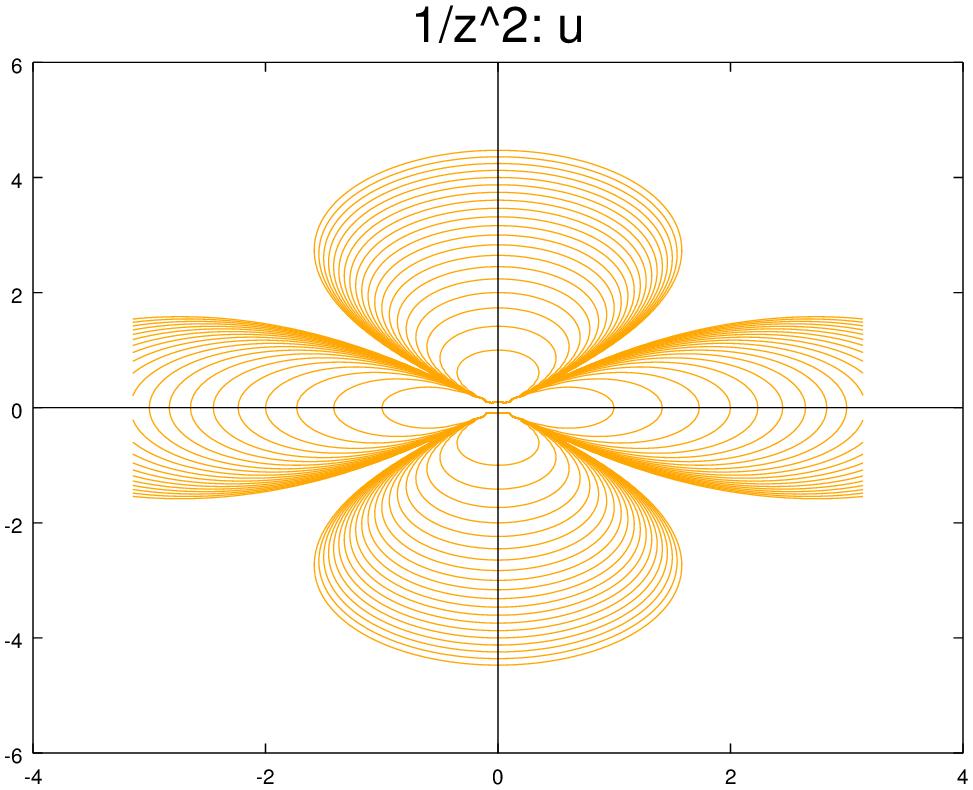
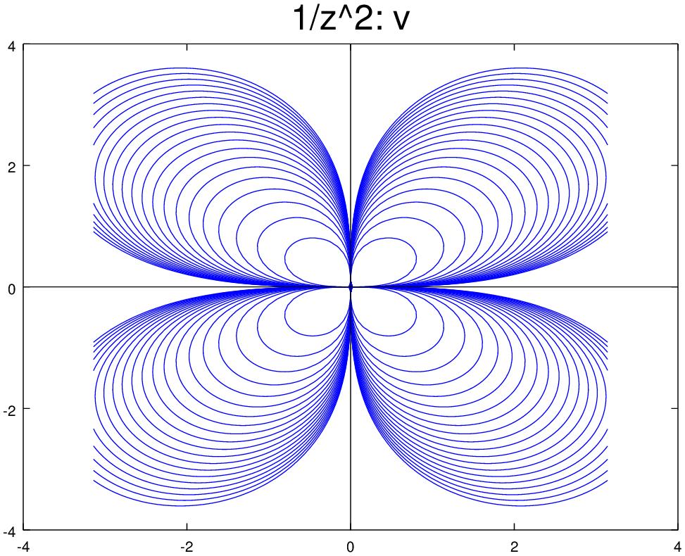
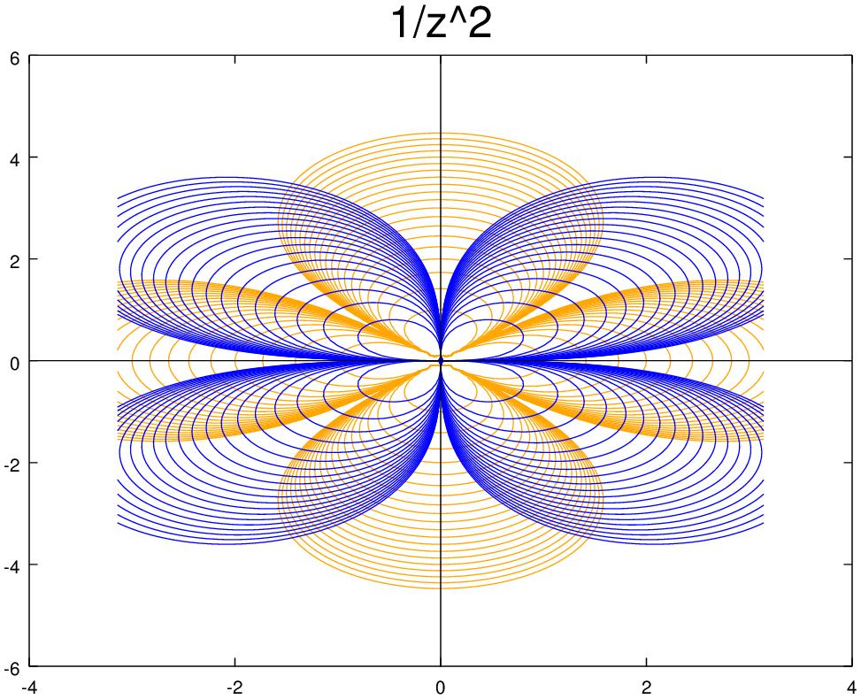
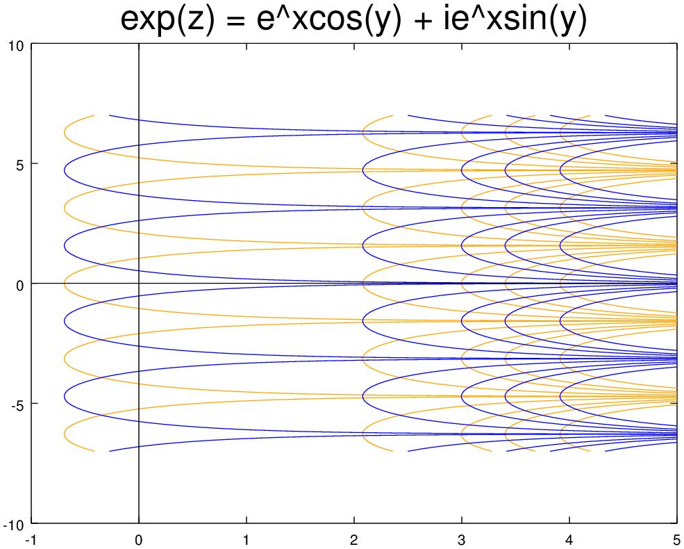
70 5 INTRODUTION TO HARMONI FUNTIONS 70

71 5 INTRODUTION TO HARMONI FUNTIONS 7 Example 5.6. Let s work out the gradients in a few simple examples. (i) Let f(z) = z 2 = (x 2 y 2 ) + i2xy. So u = (2x, 2y) and v = (2y, 2x). It s trivial to check that u v = 0, so they are orthogonal. (ii) Let f(z) = z = x r 2 i y. So, it s easy to compute r2 ( y 2 x 2 u = r 4, 2xy ) r 4 and v = ( 2xy r 4, y2 x 2 ) r 4. Again it s trivial to check that u v = 0, so they are orthogonal. Example 5.7. (Degenerate points: f (z) = 0.) onsider f(z) = z 2. From the previous example we have u(x, y) = x 2 y 2, v(x, y) = 2xy, u = (2x, 2y), v = (2y, 2x). At z = 0, the gradients are both 0 so the theorem on orthogonality doesn t apply Let s look at the level curves through the origin. The level curve (really the level set ) for u = x 2 y 2 = 0 is the pair of lines y = ±x. At the origin this is not a smooth curve. Look at the figures for z 2 above. It does appear that away from the origin the level curves of u intersect the lines where v = 0 at right angles. The same is true for the level curves of v and the lines where u = 0. You can see the degeneracy forming at the origin: as the level curves head towards 0 they get pointier and more right angled. So the level curve u = 0 is more properly thought of as four right angles. The level curve of u = 0, not knowing which leg of v = 0 to intersect orthogonally takes the average and comes into the origin at 45.

72 6 TWO DIMENSIONAL HYDRODYNAMIS AND OMPLEX POTENTIALS Appendix 5.7. Interchanging limits In our proof that the parts of an analytic function are harmonic based on auchy s theorem we needed the following. For z = x + iy write w z = u(x, y, w) + iv(x, y, w) We know that on the circle r : w z = r, u and v have derivatives of all orders in x and y. (And w, but we only care that it s continuous for w on r. Then, if f(w) is continuous on r we have x r f(w) w z dw = x f(w)u(x, y, w)+if(w)v(x, y, w) dw = f(w)u x (x, y, w)+if(w)v x (x, y, w) dw. r r That is, we can interchange the order of integration over w and taking partials in x and y. Proof. To be completed The basic idea is to see that since f(w) is bounded on r we have ( ) u(x, y0, w) u(x 0, y 0, w) lim f(w) u x (x 0, y 0 ) dw = 0. x x 0 r x x 0 6 Two dimensional hydrodynamics and complex potentials 6. Introduction Laplace s equation and harmonic functions show up in many physical models. As we have just seen, harmonic functions in two dimensions are closely linked with complex analytic functions. In this section we will exploit this connection to look at two dimensional hydrodynamics, i.e. fluid flow. Since static electric fields and steady state temperature distributions are also harmonic, the ideas and pictures we use can be repurposed to cover these topics as well. 6.2 Velocity fields Suppose we have water flowing in a region A of the plane. Then at every point (x, y) in A the water has a velocity. In general, this velocity will change with time. We ll let F stand for the velocity vector field and we can write F(x, y, t) = (u(x, y, t), v(x, y, t)). The arguments (x, y, t) indicate that the velocity depends on these three variables. general, we will shorten the name to velocity field. A beautiful and mesmerizing example of a velocity field is at html. This shows the current velocity of the wind at all points in the continental U.S. In

73 6 TWO DIMENSIONAL HYDRODYNAMIS AND OMPLEX POTENTIALS Stationary flows If the velocity field is unchanging in time we call the flow a stationary flow. In this case, we can drop t as an argument and write: F(x, y) = (u(x, y), v(x, y)) Here are a few examples. These pictures show the streamlines from similar figures in topic 5. We ve added arrows to indicate the direction of flow. Example 6.. Uniform flow. F = (, 0). Example 6.2. Eddy (vortex) F = (y/r 2, x/r 2 ) Example 6.3. Source F = (x/r 2, y/r 2 ) 6.4 Physical assumptions, mathematical consequences 6.4. Summary: mathematical consequence of physical assumptions This is a wordy section, so we ll start by listing the mathematical properties that will follow from our assumptions about the velocity field F = u + iv.

74 6 TWO DIMENSIONAL HYDRODYNAMIS AND OMPLEX POTENTIALS 74 (A) F = F(x, y) is a function of x,y, but not time t. (B) divf = 0 (divergence free). () curlf = 0 (curl free) Physical assumptions We will make some standard physical assumptions. These don t apply to all flows, but they do apply to a good number of them and they are a good starting point for understanding fluid flow more generally. More important to 8.04, these are the flows that are readily susceptible to complex analysis. Here are the assumptions about the flow, we ll discuss them further below: (A) Stationary. (B) Incompressible. () Irrotational (B) Incompressibile. We will assume that the fluid is incompressible. This means that the density of the fluid is constant across the domain. Mathematically this says that the velocity field F must be divergence free, i.e. for F = (u, v): divf F = u x + v y = 0. To understand this, recall that the divergence measures the infinitesimal flux of the field. If the flux is not zero at a point (x 0, y 0 ) then near that point the field looks like Left: Divergent field: divf > 0, right: onvergent field: divf < 0 If the field is diverging or converging then the density must be changing! That is, the flow is not incompressible. As a fluid flow the left hand picture represents a source and the right represents a sink. In electrostatics where F expresses the electric field, the left hand picture is the field of a positive charge density and the right is that of a negative charge density. If you prefer a non-infinitesimal explanation, we can recall Green s theorem in flux form. It says that for a simple closed curve and a field F = (u, v), differentiable on and inside, the flux of F through satisfies Flux of F across = F n ds = divf dx dy, where R is the region inside. Now, suppose that divf(x 0, y 0 ) > 0, then divf(x, y) > 0 for all (x, y) close to (x 0, y 0 ). So, choose a small curve around (x 0, y 0 ) such that divf > 0 on and inside. By Green s theorem Flux of F through = divf dx dy > 0. R R

75 6 TWO DIMENSIONAL HYDRODYNAMIS AND OMPLEX POTENTIALS 75 learly, if there is a net flux out of the region the density is decreasing and the flow is not incompressible. The same argument would hold if divf(x 0, y 0 ) < 0. We conclude that incompressible is equivalent to divergence free. () Irrotational. We will assume that the fluid is irrotational. This means that the there are no infinitesimal vortices in A. Mathematically this says that the velocity field F must be curl free, i.e. for F = (u, v): curlf F = v x u y = 0. To understand this, recall that the curl measures the infinitesimal rotation of the field. Physically this means that a small paddle placed in the flow will not spin as it moves with the flow Examples Example 6.4. The eddy is irrotational! The eddy from Example 6.2 is irrotational. The vortex at the origin is not in A = {0} and you can easily check that curlf = 0 everywhere in A. This is not physically impossible: if you placed a small paddle wheel in the flow it would travel around the origin without spinning! Example 6.5. Shearing flows are rotational. Here s an example of a vector field that has rotation, though not necessarily swirling. Im(z) Re(z) Shearing flow: box turns because current is faster at the top. The field F = (ay, 0) is horizontal, but curlf = a 0. Because the top moves faster than the bottom it will rotate a square parcel of fluid. The minus sign tells you the parcel will rotate clockwise! This is called a shearing flow. The water at one level will be sheared away from the level above it Summary F(x, y) = (u(x, y), v(x, y)). (A) Stationary: F depends on x, y, but not t. (B) Incompressible: divergence free, divf = u x + v y = 0, i.e. u x = v y. () Irrotational: curl free, curlf = v x u y = 0, i.e. u y = v x. For future reference we put these equalities in a numbered equation: u x = v y and u y = v x (6) These look almost like the auchy-riemann equations (with sign differences)!

76 6 TWO DIMENSIONAL HYDRODYNAMIS AND OMPLEX POTENTIALS omplex potentials There are different ways to do this. We ll start by seeing that every complex analytic function leads to an irrotational, incompressible flow. Then we ll go backwards and see that all such flows lead to an analytic function. We will learn to call the analytic function the complex potential of the flow. Annoyingly, we are going to have to switch notation. Because u and v are already taken by the vector field F, we will call our complex function Φ = φ + iψ Analytic functions give us incompressible, irrotational flows Let Φ(z) be an analytic function on a region A. For z = x + iy we write From this we can define a vector field Φ(z) = φ(x, y) + iψ(x, y). F = φ = (φ x, φ y ) = (u, v), here we mean that u and v are defined by φ x and φ y. From our work on analytic and harmonic functions we can make a list of properties of these functions.. φ and ψ are both harmonic. 2. The level curves of φ and ψ are orthogonal. 3. Φ = φ x iφ y. 4. F is divergence and curl free (proof just below). Thus the analytic function Φ has given us an incompressible, irrotational vector field F. It is standard terminology to call φ a potential function for the vector field F. We will also call Φ a complex potential function for F. The function ψ will be called the stream function of F (the name will be explained soon). The function Φ will be called the complex velocity. Proof. (F is curl and divergence free.) This is an easy consequence of the definition. curlf = v x u y = φ yx φ xy = 0 divf = u x + v y = φ xx + φ yy = 0 (since φ is harmonic). We ll postpone examples until after deriving the complex potential from the flow Incompressible, irrotational flows always have a complex potential functions For technical reasons we need to add the assumption that A is simply connected. This is not usually a problem because we often work locally in a disk around a point (x 0, y 0 ).

77 6 TWO DIMENSIONAL HYDRODYNAMIS AND OMPLEX POTENTIALS 77 Theorem. Assume F = (u, v) is an incompressible, irrotational field on a simply connected region A. Then there is an analytic function Φ which is a complex potential function for F. Proof. We have done all the heavy lifting for this in previous topics. The key is to use the property Φ = u iv to guess Φ. Working carefully we define g(z) = u iv Step. Show that g is analytic. Keeping the signs straight, the auchy Riemann equations are u x = ( v) y and u y = ( v) x = v x. But, these are exactly the equations in Equation 6. Thus g(z) is analytic. Step 2. Since A is simply connected, auchy s theorem says that g(z) has an antiderivative on A. We call the antiderivative Φ(z) Step 3. Show that Φ(z) is a complex potential function for F. This means we have to show that if we write Φ = φ + iψ, then F = φ. To do this we just unwind the definitions. Φ = φ x iφ y (standard formula for Φ ) Φ = g = u iv (definition of Φ and g) omparing these equations we get φ x = u, φ y = v. But this says precisely that φ = F. QED ( x Example 6.6. Source fields. The vector field F = a r 2, y ) r 2 models a source pushing out water or the 2D electric field of a positive charge at the origin. If you prefer a 3D model, it is the field of an infinite wire along with uniform charge density along the z-axis Show that F is curl and divergence free and find its complex potential. We could compute directly that this is curl and divergence free away from 0. An easier method is to look for a complex potential Φ. If we can find one then this will show F is curl and divergence free and find φ and ψ all at once. If there is no such Φ then we ll know that F is not both curl and divergence free. One standard method is to use the formula for Φ : Φ = u iv = This is analytic and we have Φ(z) = log(z). (x iy) r 2 = z (z z) = z.

78 6 TWO DIMENSIONAL HYDRODYNAMIS AND OMPLEX POTENTIALS Stream functions In everything we did above poor old ψ just tagged along as the harmonic conjugate of the potential function φ. Let s turn our attention to it and see why it s called the stream function. Theorem. Suppose that Φ = φ + iψ is the complex potential for a velocity field F. Then the fluid flows along the level curves of ψ, That is, the F is everywhere tangent to the level curves of ψ. The level curves of ψ are called streamlines and ψ is called the stream function. Proof. Again we have already done most of the heavy lifting to prove this. Since F is the velocity of the flow at each point, the flow is always tangent to F. You also need to remember that φ is perpendicular to the level curves of φ. So we have:. The flow is parallel to F. 2. F = φ, so the flow is orthogonal to the level curves of φ. 3. Since φ and ψ are harmonic conjugates, the level curves of ψ are orthogonal to the level curves of φ. ombining 2 and 3 we see that the flow must be along the level curves of ψ Examples We ll illustrate the streamlines in a series of examples that start be defining the complex potential for a vector field. Example 6.7. Uniform flow Let Φ(z) = z. Find F and draw a plot of the streamlines. Indicate the direction of the flow. answer: Φ = x + iy. So φ = x and F = φ = (, 0), which says the flow has uniform velocity and points to the right. We also have ψ = y, so the streamlines are the horizontal lines y = constant. Uniform flow to the right. Note that another way to see that the flow is to the right is to check the direction that the potential φ increases. The topic 5 notes show pictures of this complex potential which show both the streamlines and the equipotential lines. Example 6.8. Linear source Let Φ(z) = log(z). Find F and draw a plot of the streamlines. Indicate the direction of the flow. answer: Φ = log(r) + iθ. So φ = log(r) and F = φ = (x/r 2, y/r 2 ), which says the flow is radial and decreases in speed as it gets farther from the origin. The field is not defined at

79 6 TWO DIMENSIONAL HYDRODYNAMIS AND OMPLEX POTENTIALS 79 z = 0. We also have ψ = θ, so the streamlines are rays from the origin. Linear source: radial flow from the origin Stagnation points A stagnation point is one where the velocity field is 0. Stagnation points. If Φ is the complex potential for a field F then the stagnation points F = 0 are exactly the points z where Φ (z) = 0. Proof. This is clear since F = (φ x, φ y ) and Φ = φ x iφ y. Example 6.9. Stagnation points. Draw the streamlines and identify the stagnation points for the potential Φ(z) = z 2. answer: (We drew the level curves for this in topic 5.) We have Φ = (x 2 y 2 )+i2xy. So the streamlines are the hyperbolas: 2xy = constant. Since φ = x 2 y 2 increases as x increases and decreases as y increases, the arrows, which point in the direction of increasing φ, are as shown on the figure below. Stagnation flow: stagnation point at z = 0. The stagnation points are the zeros of Φ (z) = 2z, i.e. the only stagnation point is at the z = 0. Note. The stagnation points are what we called the critical points of a vector field in More pretty pictures Example 6.0. Linear vortex. Analyze the flow with complex potential function Φ(z) = i log(z). answer: Multiplying by i switches the real and imaginary parts of log(z) (with a sign change). We have Φ = θ + i log(r). The stream lines are the curves log(r) = constant, i.e.

80 6 TWO DIMENSIONAL HYDRODYNAMIS AND OMPLEX POTENTIALS 80 circles with center at z = 0. The flow is clockwise because the potential φ = θ increases in the clockwise direction. Linear vortex. This flow is called a linear vortex. We can find F using Φ. Φ = i z = y r 2 + x r 2 = φ x iφ y. So F = (φ x, φ y ) = ( y/r 2, x/r 2 ) by now this should be a familiar vector field. There are no stagnation points, but there is a singularity at the origin. Example 6.. Double source. Analyze the flow for with complex potential function Φ(z) = log(z ) + log(z + ). answer: This is a flow with linear sources at ±. We used Octave to plot the level curves of ψ = Im(Φ). We can analyze this flow further as follows. Two sources.. Near each source the flow looks like a linear source. 2. On the y-axis the flow is along the axis. That is, the y-axis is a streamline. It s worth seeing three different ways of arriving at this conclusion. Reason : By symmetry of vector fields associated with each linear source, the x components cancel and the combined field points along the y-axis. Reason 2: We can write Φ(z) = log(z ) + log(z + ) = log((z )(z + )) = log(z 2 ). So Φ (z) = 2z/(z 2 ). On the imaginary axis Φ (iy) = 2iy/( y 2 ). Thus, F = (0, 2y/(y 2 + )) which is along the axis. Reason 3: On the imaginary axis Φ(iy) = log( y 2 ). Since this has constant imaginary part, the axis is a streamline.

81 7 TAYLOR AND LAURENT SERIES 8 Because of the branch cut for log(z) we should probably be a little more careful here. First note that the vector field F comes from Φ = 2z/(z 2 ), which doesn t have a branch cut. So we shouldn t really have a problem. Now, as z approaches the y-axis from one side or the other, the argument of log(z 2 ) approaches either π or π. That is, as such limits, the imaginary part is constant. So the streamline on the y-axis is the limit case of streamlines near the axis. Since Φ (z) = 0 when z = 0, the origin is a stagnation point. This is where the fields from the two sources exactly cancel each other. Example 6.2. A source in uniform flow. onsider the flow with complex potential Φ(z) = z + Q 2π log(z). This is a combination of uniform flow to the right and a source at the origin. The figure below was drawn using Octave. It shows that the flow looks like a source near the origin. Farther away from the origin the flow stops being radial and is pushed to the right by the uniform flow. A source in uniform flow. Since the components of Φ and F are the same except for signs, we can understand the flow by considering Φ (z) = + Q 2πz. Near z = 0 the singularity of /z is most important and Φ Q/(2πz). So, the vector field looks a linear source. Far away from the origin the /z term is small and Φ (z), so the field looks like uniform flow. Setting Φ (z) = 0 we find one stagnation point z = Q/(2π). It is the point on the x-axis where the flow from the source exactly balances that from the uniform flow. For bigger values of Q the source pushes fluid farther out before being overwhelmed by the uniform flow. That is why Q is called the source strength. 7 Taylor and Laurent series 7. Introduction We originally defined an analytic function as one where the derivative, defined as a limit of ratios, existed. We went on to prove auchy s theorem and auchy s integral formula.

82 7 TAYLOR AND LAURENT SERIES 82 These revealed some deep properties of analytic functions, e.g. the existence of derivatives of all orders. Our goal in this topic is to express analytic functions as infinite power series. This will lead us to Taylor series. When a complex function has an isolated singularity at a point we will replace Taylor series by Laurent series. Not surprisingly we will derive these series from auchy s integral formula. Although we come to power series representations after exploring other properties of analytic functions, they will be one of our main tools in understanding and computing with analytic functions. 7.2 Geometric series Having a detailed understanding of geometric series will enable us to use auchy s integral formula to understand power series representations of analytic functions. We start with the definition: Definition. A finite geometric series has one of the following (all equivalent) forms. S n = a( + r + r 2 + r r n ) = a + ar + ar 2 + ar ar n n n = ar j = a j=0 j=0 r j The number r is called the ratio of the geometric series because it is the ratio of consecutive terms of the series. Theorem. The sum of a finite geometric series is given by S n = a( + r + r 2 + r r n ) = a( rn+ ). (7) r Proof. This is a standard trick that you ve probably seen before. S n = a+ ar + ar ar n rs n = ar + ar ar n +ar n+ When we subtract these two equations most terms cancel and we get S n rs n = a ar n+ Some simple algebra now gives us the formula in Equation 7. Definition. An infinite geometric series has the same form as the finite geometric series except there is no last term: S = a + ar + ar = a r j. Note. We will usually simply say geometric series instead of infinite geometric series. j=0

83 7 TAYLOR AND LAURENT SERIES 83 Theorem. If r < then the infinite geometric series converges to S = a r j = j=0 a r (8) If r then the series does not converge. Proof. This is an easy consequence of the formula for the sum of a finite geometric series. Simply let n in Equation 7. Note. We have assumed a familiarity with convergence of infinite series. We will go over this in more detail in the appendix to this topic onnection to auchy s integral formula auchy s integral formula says f(z) = f(w) dw. Inside the integral we have the 2πi w z expression /(w z) which looks a lot like the sum of a geometric series. We will make frequent use of the following manipulations of this expression. w z = w z/w = ( + (z/w) + (z/w) ) (9) w The geometric series in this equation has ratio z/w. Therefore, the series converges, i.e. the formula is valid, whenever z/w <, or equivalently when z < w. w z = z w/z = ( + (w/z) + (w/z) ) (20) z The series converges, i.e. the formula is valid, whenever w/z <, or equivalently when z > w. 7.3 onvergence of power series When we include powers of the variable z in the series we will call it a power series. In this section we ll state the main theorem we need about the convergence of power series. Technical details will be pushed to the appendix for the interested reader. Theorem 7.. onsider the power series f(z) = a n (z z 0 ) n. There is a number R 0 such that:. If R > 0 then the series converges absolutely to an analytic function for z z 0 < R. 2. The series diverges for z z 0 > R R is called the radius of convergence. The disk z z 0 < R is called the disk of convergence. n=0 3. The derivative is given by term-by-term differentiation f (z) = na n (z z 0 ) n n=0

84 7 TAYLOR AND LAURENT SERIES 84 The series for f also has radius of convergence R. 4. If γ is a bounded curve inside the disk of convergence then the integral is given by term-by-term integration f(z) dz = a n (z z 0 ) n Notes. γ n=0 The theorem doesn t say what happens when z z 0 = R. If R = the function f(z) is entire. If R = 0 the series only converges at the point z = z 0. In this case, the series does not represent an analytic function on any disk around z 0. Often (not always) we can find R using the ratio test. The proof of this theorem is in the appendix. γ 7.3. Ratio test and root test Here are two standard tests from calculus on the convergence of infinite series Ratio test. onsider the series 0 c n. If L = lim n c n+ /c n exists, then:. If L < then the series converges absolutely. 2. If L > then the series diverges. 3. If L = then the test gives no information. Note. In words, L is the limit of the absolute ratios of consecutive terms. Again the proof will be in the appendix. (It boils down to comparison with a geometric series.) Example 7.2. onsider the geometric series + z + z 2 + z The limit of the absolute ratios of consecutive terms is z n+ L = lim n z n = z Thus, the ratio test agrees that the geometric series converges when z <. We know this converges to /( z). Note, the disk of convergence ends exactly at the singularity z =. z n Example 7.3. onsider the series f(z) =. The limit from the ratio test is n! n=0 z n+ /(n + )! L = lim n z n = lim z /n! n + = 0. Since L < this series converges for every z. Thus, by Theorem 7., the radius of convergence for this series is. That is, f(z) is entire. Of course we know that f(z) = e z. Root test. onsider the series 0 c n. If L = lim n c n /n exists, then:

85 7 TAYLOR AND LAURENT SERIES 85. If L < then the series converges absolutely. 2. If L > then the series diverges. 3. If L = then the test gives no information. Note. In words, L is the limit of the nth roots of the (absolute value) of the terms. The geometric series is so fundamental that we should check the root test on it. Example 7.4. onsider the geometric series + z + z 2 + z The limit of the nth roots of the terms is L = lim n zn /n = lim z = z Happily, the root test agrees that the geometric series converges when z <. 7.4 Taylor series The previous section showed that a power series converges to an analytic function inside its disk of convergence. Taylor s theorem completes the story by giving the converse: around each point of analyticity an analytic function equals a convergent power series. Theorem 7.5. (Taylor s theorem) Suppose f(z) is an analytic function in a region A. Let z 0 A. Then, f(z) = a n (z z 0 ) n, n=0 where the series converges on any disk z z 0 < r contained in A. Furthermore, we have formulas for the coefficients We call the series the power series representing f around z 0. a n = f (n) (z 0 ) (2) n! = f(z) dz (22) 2πi (z z 0 ) n+ γ The proof will be given below. First we look at some consequences of Taylor s theorem. orollary. The power series representing an analytic function around a point z 0 is unique. That is, the coefficients are uniquely determined by the function f(z). Proof. Taylor s theorem gives a formula for the coefficients Order of a zero Theorem. Suppose f(z) is analytic on the disk z z 0 < r and f is not identically 0. Then there is an integer k 0 such that a k 0 and f has Taylor series around z 0 given by f(z) = (z z 0 ) k (a k + a k+ (z z 0 ) +...) = (z z 0 ) k n=k a n (z z 0 ) n k. (23)

86 7 TAYLOR AND LAURENT SERIES 86 Proof. Since f(z) is not identically 0, not all the Taylor coefficients are zero. So, we take k to be the index of the first nonzero coefficient. Theorem 7.6. Zeros are isolated. If f(z) is analytic and not identically zero then the zeros of f are isolated. By isolated we mean that we can draw a small disk around any zeros that doesn t contain any other zeros. Isolated zero at z 0 : f(z 0 ) = 0, f(z) 0 elsewhere in the disk. Proof. Suppose f(z 0 ) = 0. Write f as in Equation 23. There are two factors: (z z 0 ) k and g(z) = a k + a k+ (z z 0 ) learly (z z 0 ) k 0 if z z 0. We have g(z 0 ) = a k 0, so g(z) is not 0 on a some small neighborhood of z 0. We conclude that on this neighborhood the product is only zero when z = z 0, i.e. z 0 is an isolated 0. Definition. The integer k in Theorem 7.6 is called the order of the zero of f at z 0. Note, if f(z 0 ) 0 then z 0 is a zero of order Taylor series examples The uniqueness of Taylor series along with the fact that they converge on any disk around z 0 where the function is analytic allows us to use lots of computational tricks to find the series and be sure that it converges. Example 7.7. Use the formula for the coefficients in terms of derivatives to give the Taylor series of f(z) = e z around z = 0. answer: Since f (z) = e z, we have f (n) (0) = e 0 =. So, e z = + z + z2 2! + z3 3! +... = z n n! Example 7.8. Expand f(z) = z 8 e 3z in a Taylor series around z = 0. answer: Let w = 3z. So, Thus, f(z) = n=0 3 n n! zn+8. e 3z = e w = n=0 w n n! = k=0 n=0 3 n n! zn Example 7.9. Find the Taylor series of sin(z) around z = 0 (Sometimes the Taylor series around 0 is called the Maclaurin series.)

87 7 TAYLOR AND LAURENT SERIES 87 answer: We give two methods for doing this. Method. f (n) (0) = dn sin(z) dz n = { ( ) m for n = 2m + = odd, m = 0,, 2,... 0 for n even Method 2. Using sin(z) = eiz e iz. 2i [ sin(z) = ] (iz) n ( iz) n = 2i n! n! 2i n=0 n=0 [( ( ) n )] in z n (We need absolute convergence to add series like this.) onclusion: sin(z) = ( ) n z2n+, which converges for z <. (2n + )! n=0 Example 7.0. Expand the rational function f(z) = + 2z2 z 3 around z = 0. + z5 answer: Note that f has a singularity at 0, so we can t expect a convergent Taylor series expansion. We ll aim for the next best thing using the following shortcut. f(z) = 2( + z 2 ) z 3 + z 2 = [ z 3 2 ] + z 2. Using the geometric series we have Putting it all together n=0 n=0 + z 2 = ( z 2 ) = ( z 2 ) n = z 2 + z 4 z f(z) = z 3 ( 2 + z 2 z ) = ( z 3 + ) z n! ( ) n z 2n+ Note. The first terms are called the singular part, i.e. those with negative powers of z. The summation is called the regular or analytic part. Since the geometric series for /( + z 2 ) converges for z <, the entire series is valid in 0 < z < Example 7.. Find the Taylor series for f(z) = convergence. ez z n=0 around z = 0. Give the radius of answer: We start by writing the Taylor series for each of the factors and then multiply them out. ) f(z) = ( + z + z2 2! + z3 ( 3! z + z 2 + z ) = + ( + )z + ( + + 2! ) ( z ! + ) z ! The biggest disk around z = 0 where f is analytic is z <. Therefore, by Taylor s theorem, the radius of convergence is R =.

88 7 TAYLOR AND LAURENT SERIES 88 f(z) analytic on z <, has a singularity at z =. Example 7.2. Find the Taylor series for f(z) = around z = 5. Give the radius of z convergence. answer: We have to manipulate this into standard geometric series form. ( ( ) ( ) z 5 z 5 2 ( ) z 5 3 f(z) = 4( + (z 5)/4) = ) Since f(z) has a singularity at z = the radius of convergence is R = 4. We can also see this by considering the geometric series. The geometric series ratio is (z 5)/4. So the series converges when z 5 /4 <, i.e. when z 5 < 4, i.e. R = 4. Disk of convergence stops at the singularity at z =. Example 7.3. Find the Taylor series for f(z) = log( + z) around z = 0. Give the radius of convergence. answer: We know that f is analytic for z < and not analytic at z =. So, the radius of convergence is R =. To find the series representation we take the derivative and use the geometric series. f (z) = + z = z + z2 z 3 + z 4... Integrating term by term (allowed by Theorem 7.) we have f(z) = a 0 + z z2 2 + z3 3 z = ( ) n zn n Here a 0 is the constant of integration. We find it by evalating at z = 0. f(0) = a 0 = log() = 0. n=

89 7 TAYLOR AND LAURENT SERIES 89 Disk of convergence for log( + z) around z = 0. Example 7.4. an the series a n (z 2) n converge at z = 0 and diverge at z = 3. answer: No! We have z 0 = 2. We know the series diverges everywhere outside its radius of convergence. So, if the series converges at z = 0, then the radius of convergence is at least 2. Since 3 z 0 < 2 we would also have that z = 3 is inside the disk of convergence Proof of Taylor s theorem For convenience we restate Taylor s Theorem 7.5. Taylor s theorem. (Taylor series) Suppose f(z) is an analytic function in a region A. Let z 0 A. Then, f(z) = a n (z z 0 ) n, n=0 where the series converges on any disk z z 0 < r contained in A. Furthermore, we have formulas for the coefficients a n = f (n) (z 0 ) (24) n! = f(z) dz (25) 2πi (z z 0 ) n+ γ Proof. In order to handle convergence issues we fix 0 < r < r 2 < r. We let γ be the circle w z 0 = r 2 (traversed counterclockise). Disk of convergence extends to the boundary of A r < r 2 < r, but r and r 2 can be arbitrarily close to r. Take z inside the disk z z 0 < r. We want to express f(z) as a power series around z 0. To do this we start with the auchy integral formula and then use the geometric series. As preparation we note that for w on γ and z z 0 < r we have z z 0 < r < r 2 = w z 0, so z z 0 / w z 0 <. Therefore, w z = w z 0 (z z 0 )/(w z 0 ) = w z 0 ( ) z n z0 = n=0 w z 0 n=0 (z z 0 ) n (w z 0 ) n+

90 7 TAYLOR AND LAURENT SERIES 90 Using this and the auchy formula gives f(z) = f(w) 2πi γ w z dw = f(w) 2πi γ (w z n=0 0 ) n+ (z z 0) n dw ( ) f(w) = dw (z z 2πi (w z 0 ) n+ 0 ) n = n=0 n=0 γ f (n) (z 0 ) n! (z z 0 ) n The last equality follows from auchy s formula for derivatives. Taken together the last two equalities give Taylor s formula. QED 7.6 Singularities Definition. A function f(z) is singular at a point z 0 if it is not analytic at z 0 Definition. For a function f(z), the singularity z 0 is an isolated singularity if f is analytic on the deleted disk 0 < z z 0 < r for some r > 0. Example 7.5. f(z) = z + z 3 (z 2 has isolated singularities at z = 0, ±i. + ) Example 7.6. f(z) = e /z has an isolated singularity at z = 0. Example 7.7. f(z) = log(z) has a singularity at z = 0, but it is not isolated because a branch cut, starting at z = 0, is needed to have a region where f is analytic. Example 7.8. f(z) = has singularities at z = 0 and z = /n for n = ±, ±2,... sin(π/z) The singularities at ±/n are isolated, but the one at z = 0 is not isolated. Every neighborhood of 0 contains zeros at /n for large n. 7.7 Laurent series Theorem 7.9. (Laurent series). Suppose that f(z) is analytic on the annulus A : r < z z 0 < r 2. Then f(z) can be expressed as a series f(z) = b n (z z n= 0 ) n + n=0 a n (z z 0 ) n.

91 7 TAYLOR AND LAURENT SERIES 9 The coefficients have the formulus a n = 2πi b n = 2πi γ γ f(w) dw (w z 0 ) n+ f(w)(w z 0 ) n dw, where γ is any circle w z 0 = r inside the annulus, i.e. r < r < r 2. Furthermore The series The series a n (z z 0 ) n converges to an analytic function for z z 0 < r 2. n=0 n= b n (z z 0 ) n converges to an analytic function for z z 0 > r. Together, the series both converge on the annulus A where f is analytic. The proof is given below. First we define a few terms. Definition. The entire series is called the Laurent series for f around z 0. The series a n (z z 0 ) n is called the analytic or regular part of the Laurent series. The series n=0 n= b n is called the singular or principal part of the Laurent series. (z z 0 ) n Note. Since f(z) is not defined at z 0 we don t have any formulas for the coefficients using derivatives. Proof (Laurent series). hoose a point z in A. Now set circles and 3 close enough to the boundary that z is inside as shown. Since this curve and its interior are contained in A, auchy s integral formula says f(z) = 2πi f(w) w z dw The contour used for proving the formulas for Laurent series. The integrals over 2 cancel, so we have f(z) = 2πi 3 f(w) w z dw.

92 7 TAYLOR AND LAURENT SERIES 92 Next, we divide this into two pieces and use our trick of converting to a geometric series. The calculuations are just like the proof of Taylor s theorem. On we have z z 0 / w z 0 <, so 2πi f(w) w z dw = 2πi = 2πi = = n=0 f(w) w z 0 n=0 ( 2πi ( (z z 0 )/(w z 0 )) dw f(w) (w z 0 ) n+ (z z 0) n dw a n (z z 0 ) n. n=0 f(w) dw (w z 0 ) n+ ) (z z 0 ) n Here a n is defined by the integral formula given in the statement of the theorem. Examining the above argument we see that the only requirement on z is that z z 0 < r 2. So, this series converges for all such z. Similarly on 3 we have w z 0 / z z 0 <, so f(w) 2πi 3 w z dw = f(w) 2πi 3 z z 0 = 2πi 3 n=0 = ( 2πi n=0 = n= ( (w z 0 )/(z z 0 )) dw f(w) (z z 0 ) n+ (w z 0) n dw b n (z z 0 ) n. f(w) (w z 0 ) n dw ) (z z 0 ) n In the last equality we changed the indexing to match the indexing in the statement of the theorem. Here b n is defined by the integral formula given in the statement of the theorem. Examining the above argument we see that the only requirement on z is that z z 0 > r. So, this series converges for all such z. ombining these two formulas we have f(z) = 2πi 3 f(w) w z dw = b n (z z n= 0 ) n + n=0 a n (z z 0 ) n The last thing to note is that the integrals defining a n and b n do not depend on the exact radius of the circle of integration. Any circle inside A will produce the same values. We have proved all the statements in the theorem on Laurent series. QED 7.7. Examples of Laurent series In general, the integral formulas are not a practical way of computing the Laurent coefficients. Instead we use various algebraic tricks. Even better, as we shall see, is the fact

93 7 TAYLOR AND LAURENT SERIES 93 that often we don t really need all the coefficients and we will develop more techniques to compute those that we do need. Example Find the Laurent series for f(z) = z + around z 0 = 0. Give the region z where it is valid. answer: f(z) = +. This is a Laurent series, valid on the infinite region 0 < z <. z Example 7.2. Find the Laurent series for f(z) = z z 2 + around z 0 = i. Give the region where your answer is valid. Identify the singular (principal) part. answer: Using partial fractions we have f(z) = 2 z i + 2 z + i. Since is analytic z + i at z = i it has a Taylor series expansion. We find it using geometric series. z + i = 2i + (z i)/(2i) = ( z i ) n 2i 2i So the Laurent series is f(z) = 2 z i + 4i n=0 n=0 ( z i ) n 2i The singular (principal) part is given by the first term. 0 < z i < 2. The region of convergence is Note. We could have looked at f(z) on the region 2 < z i <. This would have produced a different Laurent series. We discuss this further in an upcoming example. Example ompute the Laurent series for f(z) = z + z 3 (z 2 on the region A : 0 < + ) z < centered at z = 0. answer: This function has isolated singularities at z = 0, ±i. Therefore it is analytic on the region A. f(z) has singularities at z = 0, ±i. At z = 0 we have f(z) = z 3 ( + z)( z2 + z 4 z ). Multiplying this out we get f(z) = z 3 + z 2 z + z + z2 z The following example shows that the Laurent series depends on the region under consideration. Example Find the Laurent series around z = 0 for f(z) = in each of the z(z ) following regions:

94 7 TAYLOR AND LAURENT SERIES 94 (i) the region A : 0 < z < (ii) the region A 2 : < z <. answer: (i) f(z) = z z = z ( + z + z2 +...) = z z z2... (ii) Since the usual geometric series for /( z) does not converge on A 2 we need a different form. f(z) = z z( /z) = ( z 2 + z + z ) Since /z < on A 2 our use of the geometric series is justified. One lesson from this example is that the Laurent series depends on the region as well as the formula for the function. 7.8 Digression to differential equations Here is a standard use of series for solving differential equations. Example Find a power series solution to the equation f (x) = f(x) + 2, f(0) = 0. answer: We look for a solution of the f(x) = a n x n. Using the initial conndition we find f(0) = 0 = a 0. Substituting the series into the differential equation we get f (x) = a + 2a 2 x + 3a 3 x = f(x) + 2 = a a x + a 2 x Equating coefficients and using a 0 = 0 we have a = a = 2 2a 2 = a, so a 2 = a /2 = 3a 3 = a 2, so a 3 = /3 4a 4 = a 3, so a 4 = /(3 4) In general (n + )a n+ = a n, so a n+ = a n (n + ) = (3 4 5 (n + ). n=0 You can check using the ratio test that this function is entire. 7.9 Poles Poles are about isolated singularities. So, we suppose f(z) is analytic on 0 < z z 0 < r and has Laurent series f(z) = b n (z z n= 0 ) n + n=0 a n (z z 0 ) n. Definition of poles. If only a finite number of the coefficients b n are nonzero we say z 0 is a finite pole of f. In this case, if b k 0 and b n = 0 for all n > k then we say z 0 is a pole of order k. If z 0 is a pole of order we say it is a simple pole of f.

95 7 TAYLOR AND LAURENT SERIES 95 If an infinite number of the b n are nonzero we say that z 0 is an essential singularity or a pole of infinite order of f. If all the b k are 0, then z 0 is called a removable singularity. That is, if we define f(z 0 ) = a 0 then f is analytic on the disk z z 0 < r. The terminology can be a bit confusing. So, imagine that I tell you that f is defined and analytic on the punctured disk 0 < z z 0 < r. Then, a priori we assume f has a singularity at z 0. But, if after computing the Laurent series we see there is no singular part we can extend the definition of f to the full disk, thereby removing the singularity. We can explain the term essential singularity as follows. If f(z) has a pole of order k at z 0 then (z z 0 ) k f(z) is analytic (has a removable singularity) at z 0. So, f(z) itself is not much harder to work with than an analytic function. On the other hand, if z 0 is an essential singularity then no algebraic trick will change f(z) into an analytic function at z Examples of poles We ll go back through many of the examples from the previous sections. Example The rational function f(z) = + 2z2 z 3 expanded to + z5 ( f(z) = z 3 + ) ( ) n z 2n+. z Thus, z = 0 is a pole of order 3. Example f(z) = z + z Example f(z) = is a simple pole. n=0 = +. Thus, z = 0 is a pole of order, i.e. a simple pole. z z z 2 + = 2 Example For the function f(z) = z(z ). (i) On the region A : 0 < z < f(z) = z + g(z), where g(z) is analytic at z = i. So, z = i z i z = z ( + z + z2 +...) = z z z2... So, for f(z) defined on this region, z = 0 is a simple pole (ii) On the region A 2 : < z < the point z = 0 is not an isolated singularity, so it makes no sense to talk about it as a pole. In general, when working with poles we will want the function to be analytic on an arbitrarily small curve, around the pole. In this example that would not be possible since the curve must always be outside the circle of radius. Example e /z = + z + z 2 2! + z So, z = 0 is an essential singularity. 3! Example log(z) has a singularity at z = 0. Since the singularity is not isolated, it can t be classified as either a pole or an essential singularity.

96 7 TAYLOR AND LAURENT SERIES Residues In preparation for discussing the residue theorem in the next topic we give the definition and a few examples here. Note well, residues have to do with isolated singularites. Definition 7.3. onsider the function f(z) with an isolated singularity at z 0, i.e. defined on 0 < z z 0 < r and with Laurent series f(z) = b n (z z n= 0 ) n + n=0 The residue of f at z 0 is b. This is denoted a n (z z 0 ) n. Res(f, z 0 ) or Res z=z 0 f = b. What is the importance of the residue? If γ is a small, simple closed curve that goes counterclockwise around b then f(z) = 2πib. γ γ is small enough to be inside z z 0 < r, and surround z 0. This is easy to see by integrating the Laurent series term by term. The only nonzero integral comes from the term b /z. Example f(z) = e /2z = + 2z has an isolated singularity at 0. From 2(2z) 2 the Laurent series we see that Res(f, 0) = / Appendix: convergence This section needs to be completed. It will give some of the careful technical definitions and arguments regarding convergence and manipulation of series. In particular it will define the notion of uniform convergence. The short description is that all of our manipulations of power series are justified on any closed bounded region. Almost, everything we did can be restricted to a closed disk or annulus, and so was valid.

97 8 RESIDUE THEOREM 97 8 Residue Theorem 8. Poles and zeros We remind you of the following terminology. Suppose f(z) is analytic at z 0 and f(z) = a n (z z 0 ) n + a n+ z n+ +..., with a n 0. Then we say f has a zero of order n at z 0. If n = we say z 0 is a simple zero. Suppose f has an isolated singularity at z 0 and Laurent series f(z) = b n (z z 0 ) n + b n (z z 0 ) n b z + a 0 + a (z z 0 ) +... which converges on 0 < z z 0 < R and with b n 0. Then we say f has a pole of order n at z 0. If n = we say z 0 is a simple pole. There are several examples in the topic 7 notes. Here is one more z + Example 8.. f(z) = z 3 (z 2 has isolated singularities at z = 0, ±i and a zero at + ) z =. We will show that z = 0 is a pole of order 3, z = ±i are poles of order and z = is a zero of order. The style of argument is the same in each case. At z = 0: f(z) = z+. all the second factor g(z). Since g(z) is analytic at z = 0 and z 3 z 2 + g(0) =, it has a Taylor series g(z) = z + z 2 + = + a z + a 2 z Therefore f(z) = z 3 + a z 2 + a This shows z = 0 is a pole of order 3. z At z = i: f(z) = z i z+. all the second factor g(z). Since g(z) is analytic at z = i, z 3 (z+i) it has a Taylor series g(z) = z + z 3 (z + i) = a 0 + a (z i) + a 2 (z i) where a 0 = g(i) 0. Therefore f(z) = a 0 z i + a + a 2 (z i) This shows z = i is a pole of order. The arguments for z = i and z = are similar. 8.2 Words: Holomorphic and meromorphic Definition. A function that is analytic on a region A is called holomorphic on A. A function that is analytic on A except for a set of poles of finite order is called meromorphic on A. z + z 2 + z 3 Example 8.2. Let f(z) =. This is meromorphic on with (z 2)(z 3)(z 4)(z 5) (simple) poles at z = 2, 3, 4, 5.

98 8 RESIDUE THEOREM Behavior of functions near zeros and poles The basic idea is that near a zero of order n, a function behaves like (z z 0 ) n and near a pole of order n, a function behaves like /(z z 0 ) n. The following make this a little more precise. Behavior near a zero. If f has a zero of order n at z 0 then near z 0, f(z) a n (z z 0 ) n, for some constant a n. Proof. By definition f has a Taylor series around z 0 of the form ( f(z) = a n (z z 0 ) n +a n+ (z z 0 ) n = a n (z z 0 ) n + a n+ (z z 0 ) + a ) n+2 (z z 0 ) a n a n Since the second factor equals at z 0, the claim follows. Behavior near a finite pole. b n (z z 0 ) n, for some constant b n. If f has a pole of order n at z 0 then near z 0, f(z) Proof. This is nearly identical to the previous argument. By definition f has a Laurent series around z 0 of the form b n f(z) = (z z 0 ) n + b n (z z 0 ) n b + a z z 0 ( b n = (z z 0 ) n + b n (z z 0 ) + b ) n 2 (z z 0 ) b n b n Since the second factor equals at z 0, the claim follows Picard s theorem and essential singularities Near an essential singularity we have Picard s theorem. We won t prove or make use of this theorem in Still, we feel it is pretty enough to warrant showing to you. Picard s theorem. If f(z) has an essential singularity at z 0 then in every neighborhood of z 0, f(z) takes on all possible values infinitely many times, with the possible exception of one value. Example 8.3. It is easy to see that in any neighborhood of z = 0 the function w = e /z takes every value except w = Quotients of functions We have the following statement about quotients of functions. statements if one or both functions has a pole instead of a zero. We could make similar Theorem. Suppose f has a zero of order m at z 0 and g has a zero of order n at z 0. Let h(z) = f(z)/g(z). Then If n > m then h(z) has a pole of order n m at z 0. If n < m then h(z) has a zero of order m n at z 0.

99 8 RESIDUE THEOREM 99 If n = m then h(z) is analytic and nonzero at z 0. We can paraphrase this as h(z) has pole of order n m at z 0. If n m is negative then the pole is actually a zero. Proof. You should be able to supply the proof. It is nearly identical to the proofs above: express f and g as Taylor series and take the quotient. Example 8.4. Let h(z) = sin(z) z 2. We know sin(z) has a zero of order at z = 0 and z 2 has a zero of order 2. So, h(z) has a pole of order at z = 0. Of course, we can see this easily using Taylor series h(z) = ( ) z 2 z z3 3! Residues In this section we ll explore calculating residues. We ve seen enough already to know that this will be useful. We will see that even more clearly when we look at the residue theorem in the next section. We introduced residues in the previous topic. We repeat the definition here for completeness. Definition. onsider the function f(z) with an isolated singularity at z 0, i.e. defined on the region 0 < z z 0 < r and with Laurent series (on that region) f(z) = b n (z z n= 0 ) n + n=0 The residue of f at z 0 is b. This is denoted a n (z z 0 ) n. Res(f, z 0 ) = b or Res z=z 0 f = b. What is the importance of the residue? If γ is a small, simple closed curve that goes counterclockwise around b then f(z) = 2πib. γ γ small enough to be inside z z 0 < r, surround z 0 and contain no other singularity of f.

100 8 RESIDUE THEOREM 00 This is easy to see by integrating the Laurent series term by term. The only nonzero integral comes from the term b /z. Example 8.5. f(z) = e /2z = + 2z has an isolated singularity at 0. From 2(2z) 2 the Laurent series we see that Res(f, 0) = /2. Example Let f(z) = z z z Res(f, 0) = z. f has a pole of order 3 at z = 0 and 2. Suppose f(z) = 2 + g(z), where g is analytic at z = 0. Then, f has a simple pole at 0 z and Res(f, 0) = Let f(z) = cos(z) = z 2 /2! Then f is analytic at z = 0 and Res(f, 0) = Let f(z) = sin(z) z = z ) (z z3 3! +... = z2 3! +... So, f has a removable singularity at z = 0 and Res(f, 0) = 0. Example 8.7. Using partial fractions. Let f(z) = z z 2. Find the poles and residues of + f. answer: Using partial fractions we write f(z) = z (z i)(z + i) = 2 z i + 2 z + i. The poles are at z = ±i. We compute the residues at each pole: At z = i: f(z) = 2 + something analytic at i. Therefore the pole is simple and z i Res(f, i) = /2. At z = i: f(z) = 2 + something analytic at i. Therefore the pole is simple and z + i Res(f, i) = /2. Example 8.8. Mild warning! Let f(z) = then we have the following Laurent z( z) expansions for f around z = 0. On 0 < z < : f(z) = z z = z ( + z + z2 +...). Thereofore the pole at z = 0 is simple and Res(f, 0) =. On < z < : f(z) = z 2 /z = ( z 2 + z + z ) Even though this is a valid Laurent expansion you must not use it to compute the residue at 0. This is because the definition of residue requires that we use the Laurent series on the region 0 < z z 0 < r. Example 8.9. Let f(z) = log( + z). This has a singularity at z =, but it is not isolated, so not a pole and therefore there is no residue at z =.

101 8 RESIDUE THEOREM Residues at simple poles Simple poles occur frequently enough that we ll study computing their residues in some detail. Here are a number of ways to spot a simple pole and compute its residue. The justification for all of them goes back to Laurent series. Suppose f(z) has an isolated singularity at z = z 0. Then we have the following properties. Property. If the Laurent series for f(z) has the form b z z 0 + a 0 + a (z z 0 ) +... then f has a simple pole at z 0 and Res(f, z 0 ) = b. Property 2 If g(z) = (z z 0 )f(z) is analytic at z 0 then z 0 is either a simple pole or a removable singularity. In either case Res(f, z 0 ) = g(z 0 ). (In the removable singularity case the residue is 0.) Proof. Directly from the Laurent series for f around z 0. Property 3. If f has a simple pole at z 0 then lim z z 0 (z z 0 )f(z) = Res(f, z 0 ) This says that the limit exists and equals the residue. onversely, if the limit exists then either the pole is simple, or f is analytic at z 0. In both cases the limit equals the residue. Proof. Directly from the Laurent series for f around z 0. Property 4. If f has a simple pole at z 0 and g(z) is analytic at z 0 then Res(fg, z 0 ) = g(z 0 ) Res(f, z 0 ). If g(z 0 ) 0 then Res(f/g, z 0 ) = g(z 0 ) Res(f, z 0). Proof. Since z 0 is a simple pole, Since g is analytic, f(z) = b z z 0 + a 0 + a (z z 0 ) g(z) = c 0 + c (z z 0 ) +..., where c 0 = g(z 0 ). Multiplying these series together it is clear that Res(fg, z 0 ) = c 0 b = g(z 0 ) Res(f, z 0 ). QED The statement about quotients f/g follows from the for products because /g is analytic at z 0. Property 5. If g(z) has a simple zero at z 0 then /g(z) has a simple pole at z 0 and Res(/g, z 0 ) = /g (z 0 ). Proof. The algebra for this is similar to what we ve done several times above. The Taylor expansion for g is g(z) = a (z z 0 ) + a 2 (z z 0 ) , where a = g (z 0 ).

102 8 RESIDUE THEOREM 02 So ( ) g(z) = a (z z 0 ) + a 2 a (z z 0 ) +... The second factor on the right is analytic at z 0 and equals at z 0. Therefore we know the Laurent expansion of /g is learly the residue is /a = /g (z 0 ). Example 8.0. Let f(z) = and compute their residues. g(z) = a (z z 0 ) ( + c (z z 0 ) +...) QED. 2 + z + z 2. Show all the poles are simple (z 2)(z 3)(z 4)(z 5) answer: The poles are at z = 2, 3, 4, 5. They are all isolated. We ll look at z = 2 the others are similar. Multiplying by z 2 we get g(z) = (z 2)f(z) = 2 + z + z 2 (z 3)(z 4)(z 5). This is analytic at z = 2 and g(z) = 8 6 = 4. So the pole is simple and Res(f, 2) = 4/3. 3 Example 8.. Let f(z) =. Find all the poles and their residues. sin(z) answer: The poles of f(z) are the zeros of sin(z), i.e. nπ for n an integer. Since the derivative sin (nπ) = cos(nπ) 0, the zeros are simple and by Property 5 above Example 8.2. Let f(z) = are simple. Res(f, nπ) = answer: learly the poles are at z = 0, ±i, 2. cos(nπ) = ( )n. z(z 2. Identify all the poles and say which ones + )(z 2) 2 At z = 0: g(z) = zf(z) is analytic at 0 and g(0) = /4. So the pole is simple and the residue is g(0) = /4. At z = i: g(z) = (z i)f(z) = is analytic at i, the pole is simple and the z(z + i)(z 2) 2 residue is g(i). At z = i: This is similar to the case z = i. The pole is simple. At z = 2: g(z) = (z 2)f(z) = z(z 2 is not analytic at 2, so the pole is not + )(z 2) simple. (It should be obvious that it s a pole of order 2.) Example 8.3. Let p(z), q(z) be analytic at z = z 0. Assume p(z 0 ) 0, q(z 0 ) = 0, q p(z) (z 0 ) 0. Find Res z=z 0 q(z). answer: Since q (z 0 ) 0, q has a simple zero at z 0. So /q has a simple pole at z 0 and Res(/q, z 0 ) = /q (z 0 )

103 8 RESIDUE THEOREM 03 Since p(z 0 ) 0 we know Res(p/q, z 0 ) = p(z 0 ) Res(/q, z 0 ) = p(z 0 )/q (z 0 ) Residues at finite poles For higher order poles we can make statements similar to those for simple poles, but the formulas and computations are more involved. The general principle is the following Higher order poles. If f(z) has a pole of order k at z 0 then g(z) = (z z 0 ) k f(z) is analytic at z 0 and if g(z) = a 0 + a (z z 0 ) +... then Res(f, z 0 ) = a k = g(k ) (z 0 ). (k )! Proof. This is clear using Taylor and Laurent series for g and f. Example 8.4. Let f(z) = sinh(z) z 5 find the residue at z = 0. answer: We know the Taylor series for sinh(z) = z + z 3 /3! + z 5 /5! +... (You can find this using sinh(z) = (e z e z )/2 and the Taylor series for e z.) Therefore, We see Res(f, 0) = 0. f(z) = z 4 3!z 2 + 5! +... Note, we could have seen this by realizing that f(z) is an even function. Example 8.5.Let f(z) = sinh(z)ez z 5 find the residue at z = 0. answer: It is clear that Res(f, 0) equals the coefficient of z 4 in the Taylor expansion of sinh(z)e z. We compute this directly as sinh(z)e z = So Res(f, 0) = /3! + /4! = 5/24. ) ) ( (z + ( z3 3! z + z2 2 + z3 3! +... = ! + ) z ! Example 8.6. Find the residue of f(z) = z(z 2 at z = 2. + )(z 2) 2 answer: g(z) = (z 2) 2 f(z) = is analytic at z = 2. So, the residue we want is the z(z 2 +) a term in its Taylor series, i.e. g (2). This is easy, if dull, to compute cot(z) Res(f, 2) = g (2) = 3 00 The function cot(z) turns out to be very useful in applications. This stems largely from the fact that it has simple poles at all multiples of π and the residue is at each pole. We show that first. Fact. f(z) = cot(z) has simple poles at nπ for n an integer and Res(f, nπ) =.

104 8 RESIDUE THEOREM 04 Proof. f(z) = cos(z). This has poles at the zeros of sin, i.e. at z = nπ. At poles f is of sin(z) the form p/q where q has a simple zero at z 0 and p(z 0 ) 0. Thus we can use the formula Res(f, z 0 ) = p(z 0) q (z 0 ). In our case, we have Res(f, nπ) = cos(nπ) = as claimed. cos(nπ) Sometimes we need more terms in the Laurent expansion of cot(z). There is no known easy formula for the terms, but we can easily compute as many as we need using the following technique. Example 8.7. ompute the first several terms of the Laurent expansion of cot(z) around z = 0. answer: Since cot(z) has a simple pole at 0 we know We also know cot(z) = b z + a 0 + a z + a 2 z cot(z) = cos(z) sin(z) = z2 /2 + z 4 /4!... z z 3 /3! + z 5 /5!... ross multiplying the two expressions we get ( ) ) b z + a 0 + a z + a 2 z (z z3 3! + z5 5!... = z2 2 + z4 4!... We can do the multiplication and equate the coefficients of like powers of z. ( b + a 0 z + b ) ( 3! + a z 2 + a ) ( 0 3! + a 2 z 3 b + 5! a ) 3! + a 3 z 4 = z2 2! + z4 4! So, b = a 0 = 0 b /3! + a = /2! a = /3 a 0 /3! + a 2 = 0 a 2 = 0 b /5! a /3! + a 3 = /4! a 3 = /45. As noted above, all the even terms are 0 as they should be. We have 8.5 auchy Residue Theorem cot(z) = z z 3 z This is one of the major theorems in It will allow us to make systematic our previous somewhat ad hoc approach to computing integrals on contours that surround singularities.

105 8 RESIDUE THEOREM 05 auchy s residue theorem. Suppose f(z) is analytic in the region A except for a set of isolated singularities. Also suppose is a simple closed curve in A that doesn t go through any of the singularities of f and is oriented counterclockwise. Then f(z) dz = 2πi residues of f inside Proof. The proof is based of the following figures. They only show a curve with two singularities inside it, but the generalization to any number of signularities is straightforward. In what follows we are going to abuse language and say pole when we mean isolated singularity, i.e. a finite order pole or an essential singularity ( infinite order pole ). The left figure shows the curve surrounding two poles z and z 2 of f. The right figure shows the same curve with some cuts and small circles added. It is chosen so that there are no poles of f inside it and so that the little circles around each of the poles are so small that there are no other poles inside them. The right hand curve is = The left hand curve is = + 4. Since there are no poles inside we have, by auchy s theorem, f(z) dz = f(z) dz = Dropping 2 and 5, which are both added and subtracted, this becomes f(z) dz = + 4 f(z) dz (26) If f(z) =... + b 2 (z z ) 2 + b z z + a 0 + a (z z ) +... is the Laurent expansion of f around z then f(z) dz = Likewise f(z) dz = 2πi Res(f, z 2 ). 6 Using these residues and the fact that = + 4, Equation 26 becomes f(z) dz = 2πi(Res(f, z ) + Res(f, z 2 )). b 2 (z z ) 2 + b z z + a 0 + a (z z ) +... dz = 2πib = 2πi Res(f, z )

106 8 RESIDUE THEOREM 06 That proves the residue theorem for the case of two poles. As we said, generalizing to any number of poles is straightforward. Example 8.8. Let f(z) = z(z 2 + ). ompute f(z) dz over each of the contours, 2, 3, 4 shown. answer: The poles of f(z) are at z = 0, ±i. Using the residue theorem we just need to compute the residues of each of these poles. At z = 0: g(z) = zf(z) = z 2 is analytic at 0 so the pole is simple and Res(f, 0) = + g(0) =. At z = i: g(z) = (z i)f(z) = is analytic at i so the pole is simple and Res(f, i) = z(z + i) g(i) = /2. At z = i: g(z) = (z + i)f(z) = is analytic at i so the pole is simple and z(z i) Res(f, i) = g( i) = /2. Using the residue theorem we have Example 8.9. ompute f(z) dz = 0 (since f is analytic inside ) 2 f(z) dz = 2πi Res(f, i) = πi 3 f(z) dz = 2πi(Res(f, i) + Res(f, 0)) = πi 4 f(z) dz = 2πi(Res(f, i) + Res(f, 0) + Res(f, i)) = 0. z =2 5z 2 z(z ) dz. answer: Let f(z) = 5z 2. The poles of f are at z = 0, and the contour encloses them z(z ) both.

107 8 RESIDUE THEOREM 07 At z = 0: g(z) = zf(z) = 5z 2 is analytic at 0 so the pole is simple and Res(f, 0) = (z ) g(0) = 2. At z = : g(z) = (z )f(z) = 5z 2 is analytic at so the pole is simple and Res(f, ) = z g() = 3. 5z 2 Finally dz = 2πi(Res(f, 0) + Res(f, )) = 0πi. z(z ) Example ompute z 2 sin(/z) dz. z = answer: Let f(z) = z 2 sin(/z). f has an isolated singularity at z = 0. Using the Taylor series for sin(w) we get ( z 2 sin(/z) = z 2 z 3!z 3 + ) 5!z 5... = z /6 z +... So, Res(f, 0) = b = /6. Thus the residue theorem gives z 2 sin(/z) dz = 2πi Res(f, 0) = π 3. z = Example 8.2. ompute dz dz, : z 2 =. z(z 2) 4 answer: Let f(z) =. The singularity at z = 0 is outside the contour of integration z(z 2) 4 so it doesn t contribute to the integral. To use the residue theorem we need to find the residue of f at z = 2. There are a number of ways to do this. Here s one: z = 2 + (z 2) = 2 + (z 2)/2 = ( z 2 ) (z 2)2 (z 2)

108 8 RESIDUE THEOREM 08 This is valid on 0 < z 2 < 2. So, f(z) = (z 2) 4 z = 2(z 2) 4 4(z 2) 3 + 8(z 2) 2 6(z 2) +... Thus, Res(f, 2) = /6 and Example ompute f(z) dz = 2πi Res(f, 2) = πi 8. dz over the contour shown. sin(z) answer: Let f(z) = / sin(z). There are 3 poles of f inside at 0, π and 2π. We can find the residues by taking the limit of (z z 0 )f(z). Each of the limits is computed using L Hospital s rule. (This is valid, since the rule is just a statement about power series. We could also have used Property 5 from the section on residues of simple poles above.) At z = 0: lim z 0 Res(f, 0) =. z sin(z) = lim z 0 cos(z) =. Since the limit exists, z = 0 is a simple pole and z π At z = π: lim z π sin(z) = lim =. Since the limit exists, z = π is a simple pole and z π cos(z) Res(f, 0) =. At z = 2π: The same argument shows Res(f, 2π) =. Now, by the residue theorem f(z) dz = 2πi(Res(f, 0) + Res(f, π) + Res(f, 2π)) = 2πi. 8.6 Residue at The residue at is a clever device that can sometimes allow us to replace the computation of many residues with the computation of a single residue. Suppose that f is analytic in except for a finite number of singularities. Let be a positively oriented curve that is large enough to contain all the singularities.

109 8 RESIDUE THEOREM 09 All the poles of f are inside Definition. We define the residue of f at infinity by Res(f, ) = f(z) dz. 2πi We should first explain the idea here. The interior of a simple closed curve is everything to left as you traverse the curve. The curve is oriented counterclockwise, so its interior contains all the poles of f. The residue theorem says the integral over is determined by the residues of these poles. On the other hand, the interior of the curve is everything outside of. There are no poles of f in that region. If we want the residue theorem to hold (which we do it s that important) then the only option is to have a residue at and define it as we did. The definition of the residue at infinity assumes all the poles of f are inside. Therefore the residue theorem implies Res(f, ) = the residues of f. To make this useful we need a way to compute the residue directly. This is given by the following theorem. Theorem. If f is analytic in except for a finite number of singularities then ( ) Res(f, ) = Res w 2 f(/w), 0. Proof. The proof is just a change of variables: w = /z. hange of variable: w = /z First note that z = /w and dz = (/w 2 ) dw. Next, note that the map w = /z carries the positively oriented z-circle of radius R to the negatively oriented w-circle of radius /R. (To see the orientiation, follow the circled points, 2, 3, 4 on in the z-plane as they are