An efficient time integration method for extra-large eddy simulations

Transcription

1 A efficiet time itegratio method for extra-large eddy simulatios M.A. Scheibeler Departmet of Mathematics

2

3 Master s Thesis A efficiet time itegratio method for extra-large eddy simulatios M.A. Scheibeler Supervisor: Prof.dr. A.E.P. Veldma Departmet of Mathematics Uiversity of Groige P.O. Box AV Groige August 005

4

5 - - Summary The calculatio of the dyamic loads o space lauchers is importat for the desig ad optimisatio of space lauchers. With aerodyamic calculatios these time-depedet aerodyamic loads could be calculated usig Extra-Large Eddy Simulatios (X-LES). X-LES simulatios solve more details of the flow physics tha Reyolds-averaged Navier Stokes (RANS), without the costs of a full Large Eddy Simulatio (LES). Noetheless, these time-accurate simulatios cost a lot of computatioal time, therefore a efficiet time itegratio method has bee desiged. It takes thousads of time steps to get statistically coverged data for X-LES. For these time steps, implicit time itegratio, based o dual time steppig method is curretly used. I the LES regio the physical (accuracy) time step is of the same order as the umerical (stability) time step. Therefore it is more efficiet to use a explicit time itegratio method, with a few relaxatios i the LES regio. The grid cells i the RANS regio, especially the boudary layer, are much smaller tha i the LES regio, hece i the RANS regio a explicit time itegratio method is ot efficiet. I the RANS regio the implicit time itegratio method based o the dual time steppig will be used, but i the LES regio the time itegratio method will be replaced with a explicit method. The couplig betwee the time itegratio method o the iterface of the RANS ad the LES regio will be desiged. The couplig that has bee desiged is secod order accurate, stable ad coservative. These aspects are aalysed i this documet. The couplig is implemeted i a multi-block Euler/Navier Stokes flow solver. Test cases show that if the implicit ad explicit regio are of the same size, the the speedup is two with respect to a fully implicit calculatio.

6 - - Cotets List of figures 5 Itroductio 7 Accuracy of discretisatio methods for the wave equatio 9. The couplig problem betwee implicit ad explicit blocks 9. Sigle step methods.. Froze poit i explicit block (Es 0 IE).. Froze poit i implicit block (IsEI) Liear extrapolatio i explicit block (E sie) 6..4 Liear extrapolatio i implicit block (I sei) 6..5 Quadratic extrapolatio i explicit block (Es IE) 7..6 Quadratic extrapolatio i implicit block (Is EI) 8..7 Extrapolatio i the implicit block (Is EI) 0.3 Predictor-Corrector methods.3. Ruge Kutta step i the implicit block (Ip RK EI c ) 3.3. Half implicit B3 step (Ip B3EI c) Lax Wedroff i the explicit regio (Ep LW IE c ) Liear extrapolatio ad explicit predictor (IsE p IE c ) Two froze poits ad explicit predictor ((IE) 0 se p IE c ) Two liear estimatios ad explicit predictor ((IE) s E pie c ) 9.4 Ruge Kutta with four stages 3.4. Ruge Kutta step i the implicit block (I RK p EI c ) U + 3 froze Oe Ruge Kutta step for U Extrapolatio of U + with U+ 4, U ad U Extrapolatio of U + with U+ 4, U ad U Extrapolatio i the implicit block (Is EI) 39.5 Couplig implicit with secod order accuracy with Ruge Kutta Ruge Kutta with two stages Liear iterpolatio Quadratic iterpolatio First order iterpolatio 4.5. Ruge Kutta with four stages 43

7 Secod order methods 45 3 Stability ad coservatio Stability aalysis Two liear estimatios ad explicit predictor ((IE) se p IE c ) Quadratic extrapolatio, (E sie) Extrapolatio i the implicit block 5 3. Coservatio Adams Bashforth predictio ((IE) se p IE c ) Step 3 for the covectio equatio ad Ruge Kutta with two stages Step 3 for the covectio equatio ad Ruge Kutta with four stages Step for the diffusio equatio Step 3 for the diffusio equatio ad Ruge Kutta with two stages Step 3 for the diffusio equatio ad Ruge Kutta with four stages Ruge Kutta o the iterface ad correctig the last stage ((IE) RK p I c E c ) Step for the covectio equatio ad Ruge Kutta with four stages Step for the diffusio equatio ad Ruge Kutta with four stages Step 3 for the covectio equatio ad Ruge Kutta with four stages Step 3 for the diffusio equatio ad Ruge Kutta with four stages Ruge Kutta o the iterface ad extrapolated fluxes ((IE) RK p Es I c ) Step for the covectio equatio ad Ruge Kutta with four stages Step for the diffusio equatio ad Ruge Kutta with four stages Stability of the coservative methods Secod order ad coservative methods 75 4 Implemetatio 77 5 Results Uiform flow o uiform grid Restartig a uiform flow with a differet agle Uiform flow o cylider grid Restartig a uiform flow o the cylider grid Flow aroud a cylider for Re = 5000, calculated with RANS Flow aroud a cylider for Re = 0 6, calculated with X-LES Order of accuracy for flow aroud a cylider for Re = 500, calculated with RANS 9

8 - 4-6 Cocludig remarks 93 7 Refereces 95 5 Tables 46 Figures Appedices 97 A Software desig 97 A. Modified procedures 99 A. New procedures 06 (07 pages i total)

9 - 5 - List of figures Figure Implicit B3 stecil. 9 Figure Explicit Ruge Kutta stecil. 0 Figure 3 Iterface problem betwee implicit ad explicit block. Figure 4 Implicit stecil with froze poit. 3 Figure 5 Explicit stecil with froze poit. 5 Figure 6 Liear extrapolatio of Ui+ + ad substituted i the B3 method. 6 Figure 7 Liear extrapolatio ad substitutio i Ruge Kutta method. 7 Figure 8 Quadratic extrapolatio ad substitutio i B3 method. 8 Figure 9 Quadratic extrapolatio ad substitutio i Ruge Kutta method. 0 Figure 0 Oe Ruge Kutta step i implicit block. 4 Figure Half implicit time step. 5 Figure Lax Wedroff ad implicit B3 method 6 Figure 3 Predictor corrector steps 7 Figure 4 Explicit method as predictor. 8 Figure 5 Two estimatios with Ruge Kutta as predictor. 30 Figure 6 Two estimatios by liear extrapolatio. 3 Figure 7 Ruge Kutta with four stages. 33 Figure 8 Ruge Kutta four o the boudary of the explicit ad implicit regio. 34 Figure 9 Ruge Kutta four o the boudary with a estimatio of U Figure 0 Ruge Kutta four o the boudary with a estimatio of U Figure Ruge Kutta four with a estimatio of the poit U Figure Ruge Kutta four with a estimatio of the poit U Figure 3 Ruge Kutta four with approximatios for U + ad U Figure 4 Grid used for stability aalysis 46 Figure 5 Figure 6 Spectral radius for differet umber of grid poits for implicit B3 (otated as im), Ruge Kutta (rk), (IE) s E pie c (ab) ad Es IE (qe) 48 Spectral radius for differet umber of grid poits for implicit B3, Ruge Kutta, (IE) se p IE c ad E sie 48 Figure 7 Eigevectors correspodig to the eigevalue, λ =, for CFL =. 49 Figure 8 Eigevector correspodig to the largest eigevalue for (IE) s E pie c 50 Figure 9 Eigevector correspodig to the largest eigevalue for Es IE 5

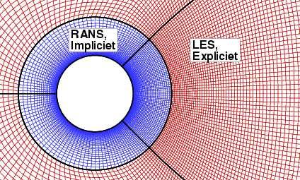
10 - 6 - Figure 30 Spectral radius for differet CFL for implicit B3 (otated as im), Ruge Kutta (rk), extrapolatio as give i equatio (36), (3) ad (34) (respectively otated as ex-im, ex ad ex) 5 Figure 3 Cotrol volumes o iterface 53 Figure 3 Iterpolatig fluxes for the last Ruge Kutta stage 55 Figure 33 Fluxes used for the implicit B3 method 60 Figure 34 Extrapolatig fluxes for the flux of the implicit domai 7 Figure 35 Spectral radius of differet CFL for the coservative methods 75 Figure 36 Residuals of uiform flow, with couplig 80 Figure 37 Residuals of uiform flow, without couplig 80 Figure 38 Residuals, restart of uiform flow with a agle of 30 degrees 8 Figure 39 Grid aroud a cylider, two times coarser 8 Figure 40 Residuals of uiform flow o cylider grid, with couplig 83 Figure 4 Residuals of uiform flow o cylider grid, without couplig 83 Figure 4 Residuals, restart of uiform flow o o-uiform grid 84 Figure 43 Lift coefficiet of flow aroud a cylider, with couplig 86 Figure 44 Lift coefficiet of flow aroud a cylider, with ad without couplig 86 Figure 45 Pressure behid a two dimesioal cylider, simulated with RANS 88 Figure 46 Turbulet Reyolds umber of a three-dimesioal cylider simulated with X-LES 9

11 - 7 - Itroductio Computig the exteral flow over space vehicles is importat for the desig ad optimisatio of space lauchers. The usteady flow emaatig from the cetral core creates usteady forces o the ozzle of a space laucher. With aerodyamic calculatios the loads o the ozzle could be calculated. These time-depedet simulatios cost a lot of computatioal time, therefore it is desirable to improve the efficiecy of the time itegratio method. For accurate calculatio of the dyamic flow, the X-LES model is used. Extra-Large Eddy Simulatio (X-LES) cosist of the Reyolds-averaged Navier Stokes (RANS) equatios with Large Eddy Simulatio (LES), where the RANS model is used i the boudary layers ad the LES model is used i the other parts of the flow. X-LES simulatios solve more details of the flow physics tha RANS, without the costs of a full LES simulatio. It takes thousads of time steps to get statistically coverged data for X-LES. Origially, implicit time itegratio is used, with the dual time steppig method cosistig of roughly a hudred relaxatios for each time step. I the LES regio the physical time step is of the same order as the umerical time step, so a explicit time itegratio, with a few relaxatios for each time step, is sufficiet. I the RANS regio, especially i the boudary layer, a explicit time itegratio method is ot efficiet. The grid cells i the RANS regio are much smaller tha i the LES regio ad if a explicit method is used i the RANS regio, a very small time step is ecessary, due to the Courat-Friedrichs-Levy (CFL) restrictio. Therefore, i the RANS regio the implicit time itegratio method, based o dual time steppig, is maitaied ad i the LES regio a explicit time itegratio method will be used. Chagig the time itegratio method o the LES regio results i a couplig of the time itegratio methods o the iterface of the RANS ad the LES regio. The iterface of the RANS ad LES regio is dyamical, but the couplig betwee the explicit ad implicit time itegratio will be o a fixed iterface. The RANS regio is approximately half the grid, coutig i grid poits, so o half the grid a explicit method will be used ad o the other half a implicit method will be used. Coutig oly the operatios of the implicit time itegratio ad eglectig the operatios of explicit time itegratio, the speedup is two with respect to oly implicit time itegratio o the grid. The couplig betwee the RANS ad the LES regio must satisfy the followig criteria: The RANS regio with the implicit time itegratio method is secod order accurate i time ad space. The low-storage Ruge Kutta scheme with four stages will be used o the LES regio. This explicit time itegratio method is secod order accurate for o-liear equatios. The couplig betwee the implicit ad explicit time itegratio methods must be secod order accurate.

12 - 8 - The implicit time itegratio method is ucoditioally stable ad the explicit time itegratio method is coditioally stable. The couplig must be as stable as the explicit time itegratio method. For correct predictio of shocks the couplig o the iterface must be coservative. The couplig betwee the RANS e LES regio is desiged for the NLR multi-block Euler/Navier Stokes flow solver ENSOLV. The flow solver ENSOLV is suitable for the simulatio of 3D, steady or time-depedet, compressible flows aroud complex aerodyamic cofiguratios. The flow equatios are the Euler ad/or Reyolds-averaged Navier Stokes equatios, cosistig of five partial differetial equatio describig the coservatio of mass, mometum ad total eergy. The turbulet flows are described with the RANS equatios; to close the RANS equatios liear eddy-viscosity models are used. The cotiuous mathematical model of the flow solver ENSOLV is described i referece 7. The flow equatios are discretised i space by a cell-cetred, fiite volume method, usig multi-block structured grids, cetral differeces ad artificial diffusio. The steady flow equatios are solved by marchig i pseudo time usig a multi-grid scheme, with explicit Ruge Kutta time itegratio as relaxatio operator. The discrete mathematical model ad solutio procedure ca be foud i referece 6. For the usteady flow equatios two solutio procedures ca be used: time accurate Ruge Kutta time itegratio ad the dual-time steppig method. The dual-time steppig method itegrates the usteady equatios i time by a secod-order implicit scheme; the resultig o-liear implicit equatios ca be solved with the steady-state solutio procedure, see referece 8. After the itroductory chapter the accuracy of several discretisatio methods for the couplig betwee the implicit ad explicit time itegratio methods will be aalysed for a model problem i chapter. Subsequetly the stability ad coservatio aalysis of several discretisatio methods is described i chapter 3. Fially, i chapter 5, the results of test cases for a solutio method with partly implicit ad partly explicit time itegratio ad a compariso with fully implicit time itegratio are preseted.

13 - 9 - Accuracy of discretisatio methods for the wave equatio This chapter discusses the discretisatio error of umerical methods for solvig the simple-wave equatio: u t = a u x. () The wave equatio is hadled such that it becomes a model problem for the couplig betwee the Reyolds-averaged Navier Stokes (RANS) ad Large Eddy Simulatio (LES) regio. The equatio will be discretised o a uiform grid with grid poits (x i,t ) ad usig a cell-cetered approach. The regio is divided ito two blocks; oe block implicitly itegratig equatio () ad the other block explicitly itegratig the equatio. To couple these two blocks, problems at the iterface appear. This results i a couplig problem betwee the two blocks.. The couplig problem betwee implicit ad explicit blocks Oe block itegrates equatio () with a implicit discretisatio method ad uses the dual time steppig method. The derivative i time is approximated usig a secod-order backward differece ad the derivative i space is approximated usig a cetral differece, which results for the iterior poits i 3U + i 4U i + U i t = a U+ i+ U+ i + τ, () x with local trucatio error τ = O( t ) + O( x ). The order of the accuracy of the implicit method is two, it is cosistet ad ucoditioally stable. This implicit method is the method of Baker ad Oliphat, or the B3-method, ad the stecil ca be see i figure. + x x t t i i i+ Fig. Implicit B3 stecil. The other block itegrates equatio () with a explicit discretisatio method; we start with Ruge Kutta with two-stages ad coefficiets α = ad α =. I subsectio.4 we also

14 - 0 - cosider Ruge Kutta with four stages. For a iterior poit, Ruge Kutta with two stages results i U + U + U t U t = a U+ U, (3) x = a U+ + U+. (4) x Substitutig equatio (3) i equatio (4) results i U + U t = a U + U x + a t U+ U + U 8 x + τ, (5) with local trucatio error τ = O( t ) + O( x ). Ruge Kutta with two-stages is a method of order two. The method is cosistet ad coditioally stable for the explicit regio. The stecil of this method ca be see i figure. + +/ / t / t x x + + Fig. Explicit Ruge Kutta stecil. Cosider the iterface betwee the implicit ad explicit block. Let poit x i lie to the left of the iterface i the implicit block. Let poit x lie to the right of the iterface i the explicit block. Near the iterface betwee the two blocks, the implicit method eeds oe poit which lies i the explicit regio ad this poit is ukow. So, if the implicit method calculates Ui + ear the iterface, the the value Ui+ + of the other block (the explicit regio) is eeded, see figure 3(a). For equatio (), this meas that Ui+ + should be replaced for a estimatio of this value. O the other had, if the explicit method is used to calculate a ew poit ear the iterface of the explicit regio, also oe poit of the other block is eeded. Particularly, if with the explicit method the value U + is calculated, the i the secod Ruge Kutta step the value U + figure 3(b). This value U + The value U + is eeded, see lies i the other block (the implicit regio) ad it is also ukow. caot be calculated with a Ruge Kutta stage, so it must be estimated i a

15 - - + x? t t i i i+ + / t +/? / t x x + + implicit explicit implicit explicit (a) Implicit stecil (b) Explicit stecil Fig. 3 Iterface problem betwee implicit ad explicit block. differet way. For equatio (4) this meas that equatio (3) ca oly be used for the value U + + ad ot for U +. This substitutio is show i equatio (6) U + U t = a U + U+ x + a t U+ U 8 x + τ. (6) Both methods, implicit ad explicit, with the discretisatio as give i equatio () ad equatio (6), respectively, require a ukow grid poit. To couple the implicit regio to the explicit regio aother discretisatio method should be cosidered.. Sigle step methods To couple the implicit regio to the explicit regio oe of the ukow grid poits, U + i+ or U+, should be approximated. Oe criterio for this couplig is that this couplig must be secod order accurate. There are several ways to couple the implicit ad explicit regio, for example usig extrapolatio or predictor-corrector schemes. This sectio cosiders discretisatio methods that take oe explicit Ruge Kutta step ad take oe implicit B3 step. If both, the Ruge Kutta step ad the implicit B3 step, are secod order accurate, the the couplig betwee the implicit ad explicit block is secod order accurate. If we take first the explicit Ruge Kutta step, the followig steps are made:. Estimate the ukow value U + (I s).. Explicit time itegratio, for calculatig the poit U + (E).

16 Implicit time itegratio, take this step if step is secod order accurate (I). First we explai the otatio of these steps. The I s meas a estimatio i the implicit block. A estimatio i the explicit block is otated as E s. A superscript of the I s or E s idicates the kid of estimatio, for example E s meas a estimatio i the explicit block of order oe. The E ad I stads for explicit ad implicit time itegratio, respectively. The estimatio of step has to be such that the explicit Ruge Kutta step (step ) is secod order accurate. With this secod order estimatio of U +, all iformatio for the implicit B3 method is available. So the implicit B3 step will also be secod order if the explicit Ruge Kutta step is secod order accurate. O the other had, if we take first the implicit B3 step, the the steps are as follows:. Estimate the ukow value Ui+ + (E s).. Implicit time itegratio, for calculatig the poit Ui + (I). 3. Explicit time itegratio, take this step if step is secod order accurate (E). The first estimatio has to be such that the implicit B3 step is secod order accurate. If the implicit B3 step is secod order accurate, the the explicit Ruge Kutta step ca be take. Step 3 still requires the ukow value U +, which must be determied by some form of iterpolatio, usig computed i step. This issue will be cosidered i subsectio.5. The ext subsectios U + i (. to.4) variates the first estimatio i the implicit regio (I s ) or the estimatio i the explicit regio (E s ). We wat these estimatios such that step, the time itegratio, is secod order... Froze poit i explicit block (E 0 s IE) First we cosider a simple approximatio of the poit (x i+,t + ) ear the iterface ad use this approximatio i the implicit method. Take the ukow value U + i+ equal to its value at time t, so U + i+ = U i+. The otatio for this estimatio is E0 s, this meas a estimatio i the explicit block of order zero. E 0 sie stads for the discretisatio with froze poit, followed by implicit ad explicit itegratio. Figure 4 shows the stecil of this estimatio with the implicit time itegratio. Substitutig the estimatio, Ui+ + = U i+, i equatio () gives 3U + i 4U i + U i t = a U i+ U+ i x + τ. (7) For the derivatio of the local trucatio error, we eed Taylor series i two variables. Suppose that u(x,t) ad all its partial derivatives of order less tha or equal to m + are cotiuous o

17 x t i i i+ implicit explicit Fig. 4 Implicit stecil with froze poit. D = {(x,t) a x b, c t d} ad let (x 0,t 0 ) D. For every (x,t) D, there exists µ betwee x ad x 0 ad ξ betwee t ad t 0 with u(x,t) = P m (x,t) + R m (x,t), where P m (x,t) = u(x 0,t 0 ) + (x x 0 ) u x (x 0,t 0 ) + (t t 0 ) u t (x 0,t 0 ) + (x x 0) u x (x 0,t 0 ) + (x x 0 )(t t 0 ) u x t (x 0,t 0 ) + (t t 0) u t (x 0,t 0 ) + + m! ( ) m m =0 (x x 0 ) m (t t 0 ) m u x m t (x 0,t 0 ) ad R m = (m + )! m+ =0 ( m + ) (x x 0 ) m+ (t t 0 ) m+ u x m+ t (µ,ξ). The fuctio P m (x,t) is the m-th Taylor polyomial i two variables ad R m (x,t) is the remaider term associated with P m (x,t), see referece. For all fuctios U i equatio (7) we calculate the Taylor series i two variables. We cosider a uiform grid with mesh size x i the x-directio ad take time steps with t. Istead of writig

18 - 4 - U(x i,t + ) i the Taylor series, we write U(x i,t + ) = Ui +. The Taylor series are with respect to (x 0,t 0 ) = (x i,t + ) ad they are as follows: U i = U + i U i+ = U + i t u t + u xi,t + t t u xi,t + 6 t3 3 t 3, µ,ξ + x u x t u xi,t + t + u xi,t + x x t x u x t + u xi,t + t t + u xi,t + 6 x3 3 x 3 xi,t + µ,ξ + t x 3 u x t µ,ξ t x 3 u x t u µ,ξ 6 t3 3 t 3, µ,ξ Ui = Ui + Ui + = Ui + t u t + t u xi,t + t xi,t t3 3 u t 3, µ,ξ x u x + u xi,t + x x u xi,t + 6 x3 3 x 3. µ,ξ With these Taylor series the derivatives i time ad space ca be estimated for the implicit B3 method with U + i+ froze. u t = 3U+ i xi,t + u x = U i+ U+ i xi,t + x Fially we fid: x 6 4U i + U i t + t x + 3 t 3 u t 3, µ,ξ u t + t u xi,t + x t t xi,t + 4 x 3 u x 3 + x t 3 u µ,ξ 4 x t t 3 u µ,ξ 4 x t + t3 µ,ξ x u t 3 u t 3 xi,t +. µ,ξ 3U + i 4U i + U i t = a U i+ U+ i x + O( t x ) + O( t) + O( x ) + O( t x). This discretisatio has bee obtaied by replacig the value Ui+ + of equatio () by the value. It is foud to be ot cosistet, because the local trucatio error does ot approach zero as U i+ t ad x approach zero i a similar way (which usually is the case, because the CFL-umbers are O()).

19 Froze poit i implicit block (I 0 s EI) I subsectio.. we approach the ukow value at time t + ear the iterface with the value oe time step earlier, at time t. A similar approach i the implicit regio ca be doe for the ukow value U +. We take U+ i the iterface equal to U. This estimatio ca be substituted i the Ruge Kutta scheme, as show i figure / / t / t x x + + implicit explicit Fig. 5 Explicit stecil with froze poit. So substitutig U + = U i equatio (6) results i: U + U t = a U + + U x a t U+ U 8 x + τ. (8) The local trucatio error ca be derived with the use of Taylor series. These Taylor series are with respect to (x 0,t 0 ) = (x,t + ). The derivative i time ad space are respectively u t u x x,t + x,t + = U+ U t = U + U x + t u t x a t u 4 x x a t x 6 t 4 x,t + x,t + 3 u t 3 µ,ξ a t U+ U 8 x x 6 a t 4 3 u x 3 t 3 u µ,ξ 8 x t u x x,t + + a t 8 x µ,ξ u t x 3 u x 3 + a t 3 u µ,ξ 8 x t a t3 3 u µ,ξ 3 x x t x,t + From here we ca coclude that the discretisatio scheme give i equatio (8) has the followig local trucatio error: τ = O( t x ) + O( t) + O( x ) + O( t x). µ,ξ

20 - 6 - The trucatio error has the order ( t x ), so this discretisatio scheme is also ot cosistet. The froze poit i the implicit regio, followed by the explicit Ruge Kutta time itegratio ad fially the implicit time itegratio is idicated as I 0 sei...3 Liear extrapolatio i explicit block (E s IE) ad U i+ A liear approximatio of the value Ui+ + i the iterface with U i+ Ui+ U i+. This extrapolatio of U+ i+ results i the discretisatio scheme: is: U+ i+ = 3U + i 4U i + U i t = a U i+ U i+ U+ i + τ, (9) x with trucatio error τ = O( t x ) + O( x ) + O( t ). O the iterface betwee the implicit ad explicit block the CFL-umber is usually chose betwee oe ad three. If t ad x are proportioally goig to zero, the this method is cosistet ad the method is first order accurate The stecil of equatio (9) is give i figure 6, the dashed arrow shows the liear extrapolatio of the poit Ui+ +. This poit is substituted i the implicit B3 method. The otatio E sie meas: first liear extrapolatio i the explicit regio, followed by implicit B3 ad explicit Ruge Kutta. + x t t i i i+ implicit explicit Fig. 6 Liear extrapolatio of U + i+ ad substituted i the B3 method...4 Liear extrapolatio i implicit block (I s EI) A liear estimatio ca also be doe i the implicit block for the value U +. The liear extrapolatio of U + is give by U+ = 3 U U. Figure 7 shows the liear extrapolatio

21 - 7 - (dashed arrow) substituted i Ruge Kutta. The substitutio of the extrapolatio of U + equatio (6) results i i U + U t = a U + 3 U + U x + a t U+ U 8 x + τ, (0) with τ = O( t x ) + O( t) + O( x ) + O( t x). The local trucatio error is of the same order as the trucatio error of the implicit method with liear extrapolatio. The explicit method with liear extrapolatio (I sei) is cosistet ad first order accurate whe the CFL-umber is O(). + +/ / t x x + + implicit explicit Fig. 7 Liear extrapolatio ad substitutio i Ruge Kutta method...5 Quadratic extrapolatio i explicit block (E s IE) First we have take a zero order extrapolatio, the a liear extrapolatio ad i this subsectio we take a quadratic extrapolatio for the value Ui+ + i the iterface of the explicit regio, we use the values Ui+,U i+. For the approximatio of U+, the value ad U i+ : i+ U + i+ = 3U i+ 3U i+ + U i+. Usig this quadratic extrapolatio i the implicit B3 method gives a secod order discretisatio scheme 3U + i 4U i + U i t = a 3U i+ 3U i+ + U i+ U+ i + τ, () x

22 - 8 - with trucatio error τ = O( t3 x ) + O( t ) + O( x ). Figure 8 shows the stecil of this method, first quadratic extrapolatio (arrow) ad the the substitutio i the B3 method. Quadratic extrapolatio followed by a implicit time step is secod order accurate. The ext step, a Ruge Kutta step i the explicit block, is worth to be take. + x t t i i i+ implicit explicit Fig. 8 Quadratic extrapolatio ad substitutio i B3 method...6 Quadratic extrapolatio i implicit block (I s EI) For the explicit block the value U + ca also be approximated usig quadratic extrapolatio: 8U + = 5U 0U + 3U. Substitutig U + i the Ruge Kutta method, equatio (6), gives the followig equatio U + U t = a 8U + 5U + 0U 3U 6 x + a t U+ U 8 x + τ, () with trucatio error τ = O( t x ) + O( t ) + O( x ) + O( t x).

23 - 9 - This method is ot secod order, but first order accurate. This will be demostrated with Taylor series. The Taylor series from the derivative i time ad space are with respect to (x 0,t 0 ) = (x,t + ) ad these derivatives are give by the followig equatio. u t u x x,t + x,t + = U+ U t t 4 3 u t 3, µ,ξ = 8U + 5U + 0U 3U 6 x + t 4 x t 6 u t + a t u 4 x x + a t x 6 x,t + + t 4 u x t x,t + a t U+ U 8 x t 6 x 3 u x t + t x 3 u µ,ξ 8 x t 7 t3 µ,ξ 48 x x,t + + a t 4 u x x,t + a t 8 x u t 3 u t 3 x,t + x 3 u µ,ξ 6 x 3 u t x x,t + 3 u x 3 a t 3 u µ,ξ 8 x t + a t3 3 u µ,ξ 3 x x t. µ,ξ µ,ξ Usig equatio () a couple of terms i the derivative i space vaish: u x x,t + = 8U + 5U + 0U 3U 6 x t 6 x + a t x 4 u t x,t + a t 8 x u t x x,t + a t U+ U 8 x + t 6 3 u x 3 7 t3 3 µ,ξ 96 x t 3 x 3 u µ,ξ 6 x 3. µ,ξ 3 u x t (3) µ,ξ From here we see that, the secod order derivatives i the Taylor series are resposible for the first order accuracy of the discretisatio. This discretisatio is show i figure 9.

24 / / t x / t x + + implicit explicit Fig. 9 Quadratic extrapolatio ad substitutio i Ruge Kutta method...7 Extrapolatio i the implicit block (Is EI) As show i subsectio..6, quadratic extrapolatio of the value U + i the Ruge Kutta method results i a first order accuracy. To get a higher accuracy we take a combiatio of U, U ad U such that with this combiatio the Ruge Kutta method becomes secod order. I other words, we extrapolate the value U + (3) vaish. such that the secod order derivatives of equatio To calculate the coefficiets of the extrapolatio, we first take a extrapolatio with three ukow parameters: U + = αu + βu + γu. To determie α, β ad γ we substitute this extrapolatio i equatio (6). The result is as follows: U + U t = a U + αu βu γu x + a t U+ U 8 x + τ. (4) With Taylor series the local trucatio error ca be estimated. The derivatives i time ad space

25 - - are: u t η u x x,t + x,t + = U+ U t t 4 3 u t 3, µ,ξ = U + αu βu γu x + ( α 3β 5γ) t 4 x + ( + α + 3β + 5γ) t 4 + ( α β γ) x u t u t x + ( α 9β 5γ) t 6 a t U+ U 8 x + a t x 6 + a t u 4 x x x,t + x,t + + ( + α + β + γ) U+ x + ( + α + β + γ) x u 4 x + ( + α + 9β + 5γ) t 6 x 3 u x 3 + ( α 3β 5γ) t x 3 u µ,ξ 8 t x 3 u t x + ( α 9β 5γ) t3 µ,ξ 96 x x,t + + a t 4 u x x,t + 3 u x 3 a t 3 u µ,ξ 8 t x + a t3 3 u µ,ξ 3 x t x, µ,ξ a t 8 x x,t + u t µ,ξ 3 u t 3 u t x x,t + µ,ξ x,t + with η = ( + α + β + γ). Rewritig the last equatio with oly the first ad secod order derivatives ad usig equatio () results i: η u x x,t + = U + αu βu γu x + ( + α + β + γ) U+ x + ( α 3β 5γ) t 4 x + ( + α + 3β + 5γ) t 4 a t U+ U 8 x + ( + α + β + γ) x 4 u t u t x + ( + α + 9β + 5γ) t 6 x x,t + x,t + u t t 4 x t 4 x,t + u t u t x + t 8 x u x x,t + x,t + u t x,t + x,t + + h.o.

26 - - To get a secod order method, the first ad secod order derivate must vaish. This gives the followig system of equatios: α + β + γ = α + 3β + 5γ = 0 α + 9β + 5γ = = α = 7 4 β = γ = 4 With the extrapolatio give i equatio (5) oly the third order derivatives are left. U + = 7 4 U U + 4 U. (5) This extrapolatio results i the followig discretisatio: U + U t = a U U + U 4 U x + a t U+ U 8 x + τ, (6) with trucatio error τ = O( t3 x ) + O( t ) + O( x ) + O( t x). Extrapolatio of the value U + as give i equatio (5) results i a Ruge Kutta method which is secod order accurate. Therefore the implicit regio ca ow take a implicit B3 step..3 Predictor-Corrector methods I the ext three subsectios the first step, the estimatio of the ukow value, is differet from the discretisatios i sectio.. Istead of extrapolatig the value at time t + or t +, the ukow value is calculated usig a discretisatio method. If we calculate the value i the iterface i the implicit block first, the three steps are as follows:. Predict the ukow value U + (I p).. Explicit time itegratio, for calculatig the poit U + (E).

27 Implicit time itegratio, take this step if step is secod order accurate (I c ). The (I p ) meas a predictio of the ukow value i the implicit regio, a superscript of I p idicates the discretisatio method that is used for the predictio. After the predictio a explicit Ruge Kutta step (E) ca be take. We require that the discretisatio o the iterface is secod order, so if step is secod order the step 3 ca be take. Step 3 corrects the predictio with a implicit B3 step (I c ). Usig a predictor i the explicit regio the steps are:. Predict the ukow value Ui+ + (E p).. Implicit time itegratio, for calculatig the poit Ui + (I). 3. Correct the predictor with Explicit time itegratio, take this step if step is secod order accurate (E c ). E p stads for the predictor i the explicit block. Step 3, the Ruge Kutta step is the corrector step. Step ad 3 must be secod order accurate, so step 3 ca be take whe step is secod order accurate..3. Ruge Kutta step i the implicit block (I RK p EI c ) We start with a predictor i the implicit block. The first step is a calculatio of the value at time t + with oe Ruge Kutta stage: U + = U a tu U. x The otatio of this predictio with oe Ruge Kutta stage is Ip RK. This results i the Ruge Kutta method with two stages, at each poit i the iterface of the explicit block, see equatio (5). The local trucatio error is: τ = O( t ) + O( x ). The calculatio of the poits i the iterface is the same as the calculatio of the iterior poits. We already kow that this method is secod order accurate (sectio.) After the Ruge Kutta method i the explicit block, the value U + becomes available. So the implicit B3 method ca take a step i the implicit block. The Ruge Kutta method ad the implicit B3 method are both secod order methods.

28 / implicit / t x + + explicit Fig. 0 Oe Ruge Kutta step i implicit block..3. Half implicit B3 step (I B3 p EI c) Oe implicit B3 time step results i a poit at a ew time t +. A implicit B3 time step from t to t + results i a poit at time t +. First we calculate U + with a half implicit B3 time step, from time t to t + Ruge Kutta step is secod order accurate, the a implicit time step calculates U +, the the Ruge Kutta step ca be take i the other block. If the The implicit time step from t to t + is show i figure (a), this results i U + = 4 3 U 3 U a t 6 x U+ 6 x U+. + a t. Substitute U + i the Ruge Kutta method, equatio (6) U + U t = a U U + 3 U x + a t 4 U U + 6 U+ 6 U+ x + τ. Usig equatio (3), the U +, U+, U + + ad U ca be elimiated. This results i: U + U t = a U U + 3 U x + a t 4 U U 6 U U + U x (7) a3 t 8 6 U U 6 U 3 x 3 + τ, with local trucatio error τ = O( t x ) + O( x ) + O( t x) + O( t ).

29 - 5 - Hece, usig a implicit step from t to t +, followed by a explicit step to time t + results i a method of first order accuracy. + +/ x + +/ / t / t / t x x + + implicit explicit + implicit explicit (a) Predictor (b) Explicit method Fig. Half implicit time step..3.3 Lax Wedroff i the explicit regio (E LW p IE c ) I this subsectio we take a predictor step i the explicit regio. For this predictio we use a discretisatio method, called Lax Wedroff. Lax Wedroff is a secod order method ad this method is used i the explicit regio, followed by the implicit B3 method. Lax Wedroff uses a substitutio for the secod order time derivative with respect to t ad therefore it becomes secod order. Usig Taylor series, the time derivative ca be rewritte: U + i u t = Ui + t u t + u t t + O( t3 ), Ui = U+ i t t u t + O( t ). (8) We write the secod order derivative i time as a derivative i space: u t u t = a u x, = a x u t = u a x. (9) Substitutio of equatio (9) i the time derivative, equatio (8), ad cetral discretisatio of u x results i: u t = U+ i Ui t a t Ui+ U i + Ui x.

30 - 6 - Cetral discretisatio of u x gives the scheme of Lax Wedroff U + i Ui t = a U i+ U i x + a t U i+ U i + U i x (0) U + i+ = U i+ + a t x U i a t x U i+ () + a t x U i+ a t x U i+ + a t x U i. Substitutig this approximatio of the value U + i+ i the implicit B3 scheme, equatio () gives 3U + i 4U i + U i t = a U i+ U+ i x a3 t 4 a t Ui Ui+ 4 x () U i+ U i+ + U i x 3 + τ, with τ = O( t3 x ) + O( x ) + O( t x) + O( t ). From this we ca coclude that this scheme is secod order. Lax Wedroff uses a substitutio of the secod order time derivative by meas of the differetial equatio (). This substitutio is easy to do for the wave equatio, but for the Navier-Stokes equatio it is difficult to do. + + x x i i+ i+ implicit explicit t t i i i+ implicit explicit (a) Lax Wedroff (b) Implicit B3 Fig. Lax Wedroff ad implicit B3 method

31 Liear extrapolatio ad explicit predictor (I s E pie c ) I the ext three subsectios the explicit Ruge Kutta method is used as predictor i the explicit block ad after the explicit method, the implicit B3 method is used. Before the Ruge Kutta method ca be used i the iterface a estimatio of the value at time t + i the implicit block must be made. The followig three subsectios variate this estimatio. The advatage of the explicit Ruge Kutta method as predictor is that i this way two times a explicit step is take ad oe times a implicit step. I cotrast, takig the implicit method as predictor, two times a implicit step is take ad oe times a explicit step. The implicit step is more expesive tha the explicit step, so takig the explicit method as predictor takes less time for oe time step. If the explicit Ruge Kutta method is used as predictor ad corrector, the four steps are:. Estimate U + i i the implicit regio (I s ).. With this estimatio a explicit time step ca be made, the result is Ui+ +. This is the predictor step, (E p ). 3. Implicit time itegratio (I), for calculatio of U + i. 4. Explicit time itegratio. This is the corrector step (E c ). These four steps are show i figure , 4 i implicit i+ explicit Fig. 3 Predictor corrector steps The iterface must be secod order accurate, this meas that step 3 ad 4 must be secod order. If step 3 is secod order accurate, step 4 ca be take. These four steps are used to derive the order of the predictor-corrector schemes with the explicit Ruge Kutta method as predictor. I the first step we use liear extrapolatio to estimate U + i U + i = 3 U i U i. This liear extrapolatio is used i the explicit Ruge Kutta method, see figure 4(a). Step, the

32 - 8 - predictor step ca be writte as: Ui+ + = Ui+ a t x U i+ + 3a t 4 x U i a t 4 x U i + a t 8 x U i+3 a t 8 x U i+. The value Ui+ + is calculated, so the implicit B3 method has all ecessary iformatio (see figure 4(b)). Usig this approximatio of Ui+ + i the implicit B3 scheme results i 3U + i 4U i + U i t = a U i+ U+ i x a t Ui+ + 3 U i U i 4 x (3) a3 t 6 U i+3 U i+ x 3 + τ, with τ = O( t3 x ) + O( x ) + O( t x) + O( t ). From here we ca coclude that liear extrapolatio (I s), followed by the explicit predictor step (E p ) ad a implicit step (I) has o secod order accuracy. + +/ / t / t + x t x x t i i+ i+ i+3 i i i+ implicit explicit implicit explicit (a) Predictor (b) Implicit stecil Fig. 4 Explicit method as predictor.

33 Two froze poits ad explicit predictor ((IE) 0 s E pie c ) I this subsectio, we are tryig to get a higher order method by takig two froze poit estimatios i the first step istead of oe froze poit estimatio. We take the explicit Ruge Kutta method as predictor ad corrector. Two estimatios results i a symmetry i the Ruge Kutta method. This symmetry takes care of removig the order t x of the Taylor series. So, two estimatios of the poits at time t + are give U + i = U i ad U + i+ = U i+. Substitutig these estimatios i the Ruge Kutta scheme, equatio (4), gives U + i+ = U i+ a t x U i+ + a t x U i. Figure 5(a) shows the predictor step. After the predictor step, Ui+ + substituted i the implicit B3 method (see figure 5(b)). is calculated, this ca be 3U + i 4U i + U i t = a U i+ U+ i x a t Ui Ui+ 4 x + τ, (4) with trucatio error τ = O( t x ) + O( x ) + O( t x) + O( t ). Two estimatios, oe i the explicit ad oe i the implicit regio ((IE) 0 s ), the Ruge Kutta method as predictor (E p ) ad a implicit time step (I) results i a first order discretisatio..3.6 Two liear estimatios ad explicit predictor ((IE) s E pie c ) I a similar way, we ca take two estimatios of the poits U + i ad U + i+ by liear extrapolatio. So, the two estimatios of the poits at time t + are give as U + i = 3 U i U i ad U + i+ = 3 U i+ U i+.

34 x +/ t implicit i i+ i+ explicit t i i i+ implicit explicit (a) Predictor (b) Implicit method Fig. 5 Two estimatios with Ruge Kutta as predictor. These estimatios are used i the Ruge Kutta method. Figure 6(a) shows the liear extrapolatio ad the Ruge Kutta step with substitutio of the poits U + i ad U + i+. Substitutig these estimatios i equatio (4) results i U + i+ = Ui+ 3a t U i+ U i x + a t U x i+ U i. (5) After the liear extrapolatios ad Ruge Kutta, the implicit B3 method ca take oe time step i the implicit block, see figure 6(b). Usig Ui+ + i of equatio (5) i the implicit B3 scheme results 3U + i 4U i + U i t = a U i+ U+ i x a t 3Ui+ + 3U i + Ui+ U i 8 x + τ. (6)

35 - 3 - With Taylor series the time ad space derivative ca calculated: u t = 3U+ i xi,t + u x = U i+ U+ i xi,t + x x 6 + a t 8 a t 4 x 4U i + U i t + t x + 3 t 3 u t 3, µ,ξ u t + t u xi,t + x t t xi,t + 4 x 3 u x 3 + x t 3 u µ,ξ 4 x t t 3 u µ,ξ 4 x t + t3 µ,ξ x 3Ui+ + 3U i + Ui+ U i x + a t x u t 3 u t 3 xi,t + µ,ξ u x + a t u xi,t + x xi,t + u t x a t 3 u xi,t + 4 x t a t3 3 u µ,ξ 8 x t x + a t x 3 u µ,ξ 3 x 3 µ,ξ Usig equatio () we ca write the space derivative as: u x = U i+ U+ i xi,t + x + a t 8 a t 4 x + t x u t + t u xi,t + x t t xi,t + 4 x 3Ui+ + 3U i + Ui+ U i x + a t x u t x + λ, xi,t + u t xi,t + u x + a t u xi,t + x xi,t + with λ = x 6 3 u x 3 t x 3 u µ,ξ t x + 5 t3 µ,ξ 4 x 3 u t 3 µ,ξ The local trucatio error of equatio (6) is give by τ = O( t3 x ) + O( x ) + O( t x) + O( t ). With two estimatios i the Ruge Kutta method the secod order derivative to time ad space of the Taylor series drops out. Oly higher order derivatives are left. Therefore this method is secod order if CFL is O(). This holds i the regio where implicit ad explicit are coupled.

36 x +/ t t t t i i+ i+ i i i+ implicit explicit implicit explicit (a) Predictor (b) Implicit method Fig. 6 Two estimatios by liear extrapolatio. The substitutio of the liear extrapolatio i the Ruge Kutta method is the same as the Adams Bashforth method. The Adams Bashforth method ca be writte for a iitial value problem as u t U + = f(u(t)) = U + t (3f(U ) f(u )). (7) For our model problem, equatio (7) is the same as equatio (5). Istead of liear extrapolatio substituted i the Ruge Kutta method, we speak of the Adams Bashforth method, because the Adams Bashforth method holds ot oly for our model problem..4 Ruge Kutta with four stages The iterior poits i the explicit block are explicitly itegrated with Ruge Kutta. Earlier we simplified the problem ad used Ruge Kutta with two stages, but i the explicit block Ruge Kutta with four stages should be used. Therefore we will exted the methods o the iterface to Ruge Kutta with four stages. The coefficiets for Ruge Kutta with four stages are α = 4, α = 3, α 3 = ad α 4 =, this results i the followig equatios U + U + U + 3 U + 4 = U a t = U a t = U a t x (U+ + U+ ) 4 x (U+ 3 + U+ 3 ) 6 x (U+ 4 + U+ 4 ) = U a t 8 x (U + U ).

37 These equatios ca be writte as U + U t = a U + U x + a t 8 x (U + U + U ) (8) a3 t 48 x 3(U +3 3U + + 3U U 3 ) + a4 t x 4(U +4 4U + + 6U 4U + U 4) + τ. With trucatio error τ = O( t 4 ) + O( x ) + O( t x ) + O( t x ). The scheme of this method ca be see i figure /3 +/ +/ Fig. 7 Ruge Kutta with four stages. The couplig betwee the implicit block ad the explicit block must be secod order. Oly the methods that are secod order o the iterface are exteded to Ruge Kutta with four stages. These methods are:. Oe Ruge Kutta stage o the iterface i the implicit block to calculate U +, Ruge Kutta i the explicit block ad implicit B3 after Ruge Kutta i the implicit block. The otatio for this method is I RK p EI c ad it is described i subsectio.3... Extrapolatio of the value U + i the implicit regio, followed by Ruge Kutta ad implicit B3, (Is EI). This extrapolatio is give i equatio (5), subsectio Implicit B3 with quadratic extrapolatio, followed by Ruge Kutta ca be used, (Es IE). These step are described i subsectio Adams Bashforth as predictor i the explicit block, the implicit B3 ad Ruge Kutta ((IE) se p IE c ). I subsectio.3.6 it is show that this method is secod order accurate. 5. Lax Wedroff i the explicit block, equatio (0), followed by implicit B3 ad a estimatio of the poit U +, fially Ruge Kutta, (E LW p IE c ), (subsectio.3.3).

38 The last three methods, Es IE, (IE) s E pie c ad Ep LW IE c, ca be exteded to Ruge Kutta with four stages i the same way. For these methods oly the estimatios betwee implicit ad explicit time itegratio i the implicit block must be chaged; this will be cosidered i sectio.5. The first two methods, (I RK p EI c ) ad (Is EI), will both be exteded i their ow way i the followig subsectios. The values U + 4 ad U+ are the ukow values i the implicit block, these values must be estimated. Leavig the values U + 4 ad U+ stages, the equatio becomes i Ruge Kutta with four U + U t = a U + U+ x + a t 8 x (U + U ) (9) a3 t 48 x 3(U +3 U+ + U + 4 ) + a4 t x 4(U +4 3U + + U ). Equatio (9) is used i the ext subsectios..4. Ruge Kutta step i the implicit block (I RK p EI c ) A Ruge Kutta step i the implicit block results for Ruge Kutta with two stages i a ormal Ruge Kutta process. Usig Ruge Kutta with four stages i the implicit block results also i the usual Ruge Kutta process with four stages as described previously. After the Ruge Kutta stages the implicit B3 method i the implicit regio ca be used ad the implicit B3 is secod order. For Ruge Kutta with four stages the stecil is wide, therefore we have to use may poits i the implicit regio, see figure /3 +/ +/ implicit explicit Fig. 8 Ruge Kutta four o the boudary of the explicit ad implicit regio. To calculate U + for Ruge Kutta with two stages, oe poit i the implicit block ad oe poit i the explicit block are ecessary. This Ruge Kutta step i the implicit block is easy to

39 execute. For Ruge Kutta with four stages this becomes more complicated, because to calculate the poit U + more poits i the implicit ad explicit blocks are ecessary. The stecil of Ruge Kutta with four stages is wide ad this aspect will be chaged i the ext subsectios. I these subsectios, we do ot use the poits i the implicit domai far from the iterface: x 3 ad x U + 3 froze For Ruge Kutta with two stages, oly the values at x ad x i the implicit regio are used. For Ruge Kutta with four stages we also wat to use the values at x ad x. Usig the value U istead of U+ 3 i Ruge Kutta with four stages, the values at x 3 ad x 4 are ot ecessary. I figure 9, a substitutio of U + 3 = U i Ruge Kutta four is show. + +/ +/3 +/ implicit explicit Fig. 9 Ruge Kutta four o the boudary with a estimatio of U +. The equatios are as follows: U + U + 4 = U a t 4 x (U+ 3 U ) = U a t 4 x (U U ) + a t 4 x (U + U ) a3 t 3 9 x 3(U + U + U ), = U a t 8 x (U U ).

40 Substitutig this i Ruge Kutta with four stages, equatio (9) results i U + U t = a U + U x + a t U+ U + U 8 x (30) a3 t 48 x 3(U +3 U + + U ) + a4 t x 4(U +4 3U + + 3U U ) + τ with trucatio error τ = O( t x ) + O( x ) + O( t 3 ). The discretisatio give i equatio (30) is first order..4.. Oe Ruge Kutta step for U + Tryig the make the method secod order, we take oe Ruge Kutta step to estimate the value U +. The stecil of this discretisatio is give i figure 0. For this discretisatio oly the values at x ad x i the implicit block are used. U + U + 4 = U a t 4 x (U U ), = U a t 8 x (U U ). Substitutig this estimatio i equatio (9) results i U + U t = a U + U x + a t U+ U + U 8 x (3) a3 t 48 x 3(U +3 U+ + U ) + a4 t x 4(U +4 3U + + 3U U ) + τ

41 with trucatio error τ = O( t x ) + O( x ) + O( t 3 ). This method is cosistet ad first order accurate. A first order accuracy of the poit U + substituted i the Ruge Kutta method with four stages, does ot result i a secod order accuracy. + +/ +/3 +/ implicit explicit Fig. 0 Ruge Kutta four o the boudary with a estimatio of U Extrapolatio of U + with U+ 4, U ad U For a estimatio of U + ot oly values at time t, but also values at time t ad t + ca be 4 used. I figure (a) a extrapolatio of U + with the poits U+ 4, U ad U is show. We take such extrapolatio of these poits, that Ruge Kutta with four stages becomes secod order. This extrapolatio is give i equatio (3). U + = 0 3 U U + 3 U, (3) U + 4 = U a t 8 x (U U ). Substitutig this extrapolatio i Ruge Kutta with four stages results i U + U t = a U + 3 U 3 U x + a t U+ 8 3 U U 8 x (33) a3 t 48 x 3(U +3 U+ + U ) + a4 t x 4(U +4 3U + + 3U U ) + τ,

42 with local trucatio error τ = O( t3 x ) + O( t ) + O( x ) + O( t x). This discretisatio gives a secod order method, but the coefficiets i the extrapolatio, equatio (3), caot be determied a priori. Sometimes the poit U + 3 diffusio is preset i the equatio, but the extrapolatio of the value U + 3 a priori from these equatios. is also ecessary, for example if caot be determied + + +/ +/4 t implicit explicit +/ +/3 +/ implicit explicit (a) Estimatio (b) Explicit method Fig. Ruge Kutta four with a estimatio of the poit U Extrapolatio of U + with U+ 4, U ad U + 4 For extrapolatio of U + also the value U( )+ 4 ca be used. The values U ( )+ 4 ad U + 4 are approximated usig a Ruge Kutta step. A secod order method with extrapolatio of these values ca be derived. This extrapolatio is give i equatio (34). U + = 3 U+ 4 3 U + 3 U( )+ 4 (34) U + 4 U ( )+ 4 = U a t 8 x (U U ) = U a t 8 x (U U ).

43 The substitutio of the extrapolatio i equatio (9) results i U + U t = a U + 3 U 3 U x + a t U+ 3U + U 3 U + 3 U 8 x (35) a3 t 48 x 3(U +3 U+ + U ) + a4 t x 4(U +4 3U + + 3U U ) + τ with τ = O( t3 x ) + O( t ) + O( x ) + O( t x). The stecil of this discretisatio is give i figure. This discretisatio is secod order, but also with this discretisatio it is difficult to approximate U / +/4 +/ +/3 +/ /4 implicit explicit implicit explicit (a) Estimatio (b) Explicit method Fig. Ruge Kutta four with a estimatio of the poit U Extrapolatio i the implicit block (Is EI) Extrapolatio of the poit U + as give i equatio (5) ad substituted i Ruge Kutta with two stages results i a secod order method. This should be exteded to Ruge Kutta with four stages. The poit U + has to be extrapolated such that the discretisatio is secod order accurate

44 ad U + 4 ca be calculated with oe Ruge Kutta stage. The followig extrapolatio results i a secod order discretisatio: U + = 3 U 4 3 U + 5 U, (36) U + 4 = U a t 8 x (U U ). Substitutig this i the Ruge Kutta method, equatio (9), results i U + U t = a U + 3 U U 5 U x + a t U+ U 8 x (37) a3 t 48 x 3(U +3 U + + U ) + a4 t x 4(U +4 3U + + 3U U ) + τ with trucatio error τ = O( t3 x ) + O( t ) + O( x ) + O( t x). The discretisatio give i equatio (37) results i a secod order method. With our equatio () we do ot eed U + 3, but sometimes this poit is also ecessary, for example by addig diffusio ito the equatio. I the implicit regio this poit should also be extrapolated, but U + 3 to derive from Taylor series..5 Couplig implicit with secod order accuracy with Ruge Kutta.5. Ruge Kutta with two stages is difficult I sectio. ad.3 a couple of discretisatios are secod order accurate, for example Ep LW IE c, EsIE ad (IE) se p IE c. Ep LW IE c, estimates the value Ui+ + i the explicit block with Lax Wedroff ad the a implicit B3 step calculates Ui +. The value Ui + is secod order accurate. I the implicit block the values at time t + ad t are kow. The Ruge Kutta method with two stages i the explicit block eeds the value U + of the implicit block, see figure 3(b). This value U + should be estimated such that Ruge Kutta is still a secod order method. I this subsectio we cosider the accuracy of the value at (x,t + ) with several iterpolatios.