Team 10 OPTIMAL DESIGN OF QUADCOPTOR By. Abstract: Preeti Vaidya ( ) Gaurav Pokharkar ( ) Nikhil Sonawane ( )

Transcription

1 1 Team 10 OPTIMAL DESIGN OF QUADCOPTOR By Preeti Vaidya ( ) Gaurav Pokharkar ( ) Nikhil Sonawane ( ) MAE 598 Final Report Abstract: This project was undertaken to study quadcopters or quad rotors which are like miniature helicopters with four rotors. Quad copters use two sets of fixed pitch propellers, two clockwise and two counter clockwise. These use variations of rpm to control torque. Control of vehicle motion is achieved by altering the rotation rates of one or more discs, thereby changing its torque load and thrust/lift characteristics. These devices are becoming increasingly popular in recent times as they offer good maneuverability, increased payload carrying capacity with simple mechanics and moderate cost as compared to actual helicopters or other UAVs. They have vast applications ranging from surveillance, disaster aid and rescue to crop survey in different parts. Current quadcopter models have persistent issues in vertical flights, torque induced control issues and high energy consumptions. Therefore, this project was outlined to study different quadcopter systems to increase the energy efficiency in the same power for given payload capacity and size constraints.

2 2 Table of Contents Table of Figures...4 Design problem statement...5 Subsystem 1: Optimization of the frame design (Gaurav Pokharkar)...6 Subsystem 2: Optimization of propulsion system (Preeti Vaidya)...6 Subsystem 3: Component placement optimization (Nikhil Sonawane)...7 Nomenclature...8 Subsystem 1: Optimization of the frame design (Gaurav Pokharkar)...8 Subsystem 2: Optimization of propulsion system (Preeti Vaidya)...9 Subsystem 3: Component placement optimization (Nikhil Sonawane) Subsystem 1: Optimization of structural frame design (Gaurav Pokharkar) Mathematical model Objective Constraints Model analysis Functional Dependency Table Monotonicity Analysis Numerical Results Optimization study Parametric Study Discussion of Results Subsystem 2: Optimization of propulsion system (Preeti Vaidya) Mathematical model Propeller design optimization: Model Analysis Optimization study Discussion of Results Motor and Battery selection Subsystem 3: Optimization of Placement of Components (Nikhil Sonawane) Mathematical model Model analysis... 35

3 3 Optimization study Parametric Study Discussion of Results System Integration System trade-offs and discussion on results: Acknowledgment References Appendix Subsystem 1: Optimization of structural frame design (Gaurav Pokharkar) Subsystem 2: Optimization of propulsion system (Preeti Vaidya) Geometry inputs Thrust torque calculations Calculate Ct and Cq and J Subsystem 3: Optimization of Placement of Components (Nikhil Sonawane) Overlap Check Main Fucntion File Objectivee Function Stacking... 74

4 Table of Figures Figure 1 Cantilever Beam Figure 2 Natural Frequency Modes of a Cantilever Beam Figure 3 Common cross sections used for frame of quadcopters Figure 4 Cross-section of the arm Figure 5 Excel output Figure 6 Objective v/s OD and ID Figure 7 Objective v/s L and ID Figure 8 Objective v/s OD and L Figure 9 Solidworks Output Figure 10 Aero foil blade profile and force balance Figure 11Flow chart to show flow of logic in design model code Figure 12 Curve fitting of Cl vs alpha data using metamodeling Figure 13 Curve fitting of Cd vs Cl data from metamodeling Figure 14 Monotonically increasing objective function wrt p/d ratio Figure 15 Plot of objective function (efficiency) wrt D and alpha Figure 16 Plot of optimum D value at various thrusts Figure 17 Plot of variation of optimum alpha wrt variation in thrust Figure 18 Objective function vs X,Y Figure 19 Objective fucntion vs X,Y Figure 20 Initial placement of components Figure 21 Optimised placment Figure 22 Closely packed components Figure 23 Optimal solution Figure 24 Optimal Solution Figure 25 Parametric Variation of function Figure 26 Components adjusted in Y direction Figure 27 CAD model of optimised quadcopter

5 5 Design problem statement As stated in the abstract current quadcopters models face issues like unsteady flight, failure of structural components and high energy consumptions during flight. These issues limit large scale use of quadcoptors. Keeping this in mind, the design problem focuses on increasing the efficiency of operation of quadcopter by improving efficiency of propulsion system, minimizing the overall weight of the frame and optimum placement of different components in a quadcopters. This project proposes a practical method to handle the design problem of a small-scale rotorcraft by combining the theoretical knowledge of the system and the result of a system level optimization analysis. The method is driven by the application. We define a target size and weight for the system and the setup a model to choose the best components to be used and estimate iteratively the most important design parameters. The subsystems we will be working upon are broadly classified into following parts- 1. Optimization of the frame design 2. Optimization of propulsion system 3. Component placement optimization and path optimization Optimization of each sub-system independently will lead to sub-optimization of the system. As all the systems are inter linked and interconnected, design of one system will affect the design of another system. Hence, to optimize the performance of the quadcopter it necessary to study the effect of all the systems on the overall performance and do trade-offs wherever required in order to get overall optimal solution.

6 6 Subsystem scope: Optimization of the frame design Analysis of frame design with different types of cross section Selection of optimal frame configuration Optimization of propulsion system Rotor Motor Battery Component placement optimization and path optimization Optimal placement of objects on frame Subsystem 1: Optimization of the frame design (Gaurav Pokharkar) The frame is the basic structure which holds all the components of the quadcopter i.e. motors, battery, control circuits, camera etc. Due to this reason its design becomes an important parameter affecting the performance of the quadcopter. The strength of the frame, its weight, its material, its configuration and various other factors are to be considered while designing the frame. We aim at optimizing the frame so as to increase strength and reduce its weight and manufacturing cost which would increase the operation time, minimize overall weight of the quadcopter giving it robustness and rigidity and also it would be economical to manufacture. Secondly, the motors and rotor rotation causes vibrations in the quadcopter frame. It is necessary to check the frame for vibrations analysis to ensure that applied frequency does not coincide with the natural modes of frequency of the frame. If this happens it will lead to resonance. Subsystem 2: Optimization of propulsion system (Preeti Vaidya) Rotor, motor and battery constitute the major components of the propulsion system. Quadrotor derives its thrust from the rotation of rotor blades such as a helicopter does. This subsystem mainly aims at introducing rotor aerodynamics and identifying methods to improve the thrust producing capacity of a quadrotor, hence improving its performance and efficiency. A fundamental and feasible route for realizing this performance improvement is identified by examining rotor selection based on theoretical models, such as the combined momentum and blade element theory, and on experimental data extracted from propulsion tests performed in the laboratory. The rotor optimization can be based either on the blade element theory or combined momentum or by performing propulsion tests. Each propulsion unit must be able to lift its own weight, one quarter of the electronics, structure and payload weight, while supplying a residual amount of

7 7 thrust sufficient for hover stability and maneuverability. Much of the design effort falls in the proper combination of the batteries, motor, and propellers to produce an efficient propulsion unit. Hence, the following propulsion component analysis is to be performed to help in their proper selection Subsystem 3: Component placement optimization (Nikhil Sonawane) Optimal placement of objects on frame Various components placed on the frame contribute to the balancing of the quadcopter which is the most important factor to be worked upon. The components mounted will not only add to the weight of the system but also affect the center of gravity which has to coincide with frame center of gravity for maximum stability. Thus figuring out the distance at which the components are placed and their exact position would play a vital role in optimizing the design of quadcopter.

8 8 Nomenclature m: Mass of the quadcopter (kg) P: Payload to be carried (kg) Mb: Battery weight (kg) I: Mass moment of inertia (kg.mm^2) Subsystem 1: Optimization of the frame design (Gaurav Pokharkar) m: Mass of the quadcopter (Kg) F: Thrust force due to motor (N) Cm: Manufacturing cost ($/m 3 ) Cr: Cost of raw material ($/kg) Cp: Cost for precision ($) L: Length of the arm (m) M: Moment due to force (F) (N-m) f: Frequency of the motors (Hz) f1, f2, f3, f4, f5: First five natural frequencies of the cantilever beam (Hz) σ: Bending stress (N/m 2 ) I: Area moment of inertia of the cross-section (m 4 ) L: Length of the arm (m) ρ: Density of the material (kg/m 3 ) E: Young s modulus (N/m 2 ) σt: Tensile strength of the material (N/m 2 ) σd: Design strength of the material (N/m 2 ) FOS: Figure of safety WR: Weight of raw material (kg) VR: Volume of material removed (m 3 )

9 9 WF: Final weight of arm (kg) OD: Outer Diameter of the arm (m) ID: Inner Diameter of the arm (m) A: Cross-section area of the beam (m 2 ) y: Distance of the outer most filament from the center (OD/2) (m) Subsystem 2: Optimization of propulsion system (Preeti Vaidya) T1, T2, T3, T4: Thrust force developed by rotors (N) T: Total thrust force developed (N) M: Torque required by individual propellers (Nm) n: Rotational speed of the rotors (rad/sec) N: Rotational speed of the rotors (rpm) V: translational velocity of quadcopter (m/s) D: diameter of propeller or rotor ρ: density of air (kg/m^3) Cp: co-efficient of power Ct: co efficient of thrust T Cq: co efficient of torque M J: advance ratio α: angle of attack (radians) θ: geometric pitch angle (radians) φ: local inflow angle p: pitch of the propeller blade Vinf: forward velocity of the quadcopters V2: angular flow velocity a: axial inflow factor

10 10 b: angular inflow factor Cl: Lift co-efficient Cd: Drag co-efficient t: time of flight to cover specified area (min) L: Maximum allowable length of arms (mm) B: maximum width of the quadcopter (mm) H: maximum height of the quadcopter (mm) h: Height at which the quadcopter is traversing C: total cost for manufacture of quadcopter ($) g: acceleration due to gravity (m/s^2) Vw: wind velocity (m/s) Subsystem 3: Component placement optimization (Nikhil Sonawane) Mx :moment about X axis ( N-mm) My: moment about Y axis ( N-mm) Xcg: X coordinate of cg of a component Ycg: Y coordinate of cg of a component g: Inequality constraints h: equality constraints

11 11 Subsystem 1: Optimization of structural frame design (Gaurav Pokharkar) Mathematical model Objective The main aim of the optimization problem is to reduce the overall weight and cost of manufacturing of the frame of the quadcopter.to minimize both cost and weight of the quadcopter we combine with higher weight assigned to the weight of the quadcopter. The objective function is as follows: min 0.25 *(Cm* VR + Cp + Cr * WR) +0.75*(WF) Material was assumed to be as Aluminum as it light in weight and also has good tensile strength. Constraints The thrust due to motor act at the tips of the arms and the weight of the quadcopter acts at the center of the frame. Hence the arms behave as cantilever beam. Initially assuming to be as 8-9 N Figure 1 Cantilever Beam The bending stress due to the thrust generated by motor should be less than the design stress. Assuming the factor of safety (FOS) to be about 2. As the beam is under bending we know, [1] M y σ = I

12 12 Also, the rod can also fail due to resonance when the natural frequency of the rod matches with that of the motor. Hence the rod should be designed in such a way that the natural frequency of the rod is different than the frequency of the motor. [2] The natural frequency of the cantilever beam is given as: [3] Figure 2 Natural Frequency Modes of a Cantilever Beam Some of the common types of cross sections are as follows:

13 13 Figure 3 Common cross sections used for frame of quadcopters SelectingHollow circular tube as the cross section of the arms as it has largest inertia for the same weight/area also it is symmetric. Hence and A = 0.25 pi (OD 2 ID 2 ) I = pi (OD4 ID 4 ) 64 Assuming that the length of the arms should be at least 200 mm so as to have enough space to mount all the components. As the material chosen is Aluminum the material properties are as follows: [4] σt = 276 MPa ρ = 2700 kg/m 3 E = 6.9e10 N/mm 2 Assuming the FOS as 2.

14 14 Hence σd = σt/2 ~ 120 N/mm 2 and σ<σd Assuming the frequency of the motor as 120 rps. Hence the natural frequency of the arm should not fall between 90 rps to 150 rps. Assuming the cost of manufacturing as: Cm = 2 $/m 3 Cp = 0.5 $ Cr = 4 $/kg From manufacturing point of view the minimum thickness of the rod should be 4 mm. Hence the optimization problem is as follows: Min 0.25 *(Cm * VR + (Cp * L/ID) + Cr * WR) * (WF) min 0.25 (C m pi ID2 L 4 + (C p L ID ) + C r pi OD2 L ) pi (OD2 ID 2 ) L ρ 4 Where CB is OD and CA is ID Subject tog1: OD-ID 4 mm g2: Figure 4 Cross-section of the arm

15 15 F L OD 64 (OD 4 ID 4 ) N mm2 g3: f1 150 rps g4: f2 150 rps g5: f3 150 rps g6: f4 150 rps g7: f5 150 rps Where, f n = a n E (OD4 ID 4 ) 4 (OD 2 ID 2 ) 64 ρ L 4 For n = 1 to 5, a1= 3.516,a2= ,a3= 61.69,a4=120.09,a5= g8: OD 4 mm g9: ID 4 mm

16 16 Model analysis Functional Dependency Table Motor Speed (rps) Material Properties OD ID L F f x x x g1 x x x g2 x x x x g3 x x x x x g4 x x x x x g5 x x x x x g6 x x x x x g7 x x x x x g8 g9 x x The functional dependency table shows the dependency of the objective and constraints on various variables and parameters.this table gives an initial idea about various interactions between the variables and the objective and constraints. The table does not include all the parameters, except yield strength of rubber, because they appear only in the objective function and not in the constraints. Monotonicity Analysis Activity analysis of the constraints was carried using monotonicity analysis. The table below gives the summary about the same. The highlighted rows shows the constraints that are active. OD ID f + - g1 - + g2 - + g3 + + g4 - - g5 - - g6 - - g7 - - g8 - g9 -

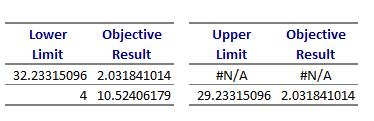
17 17 As it can be seen from the table that g1is active constraints. Also, later it can compared with the numerical results that are obtained. The Lagrange s multiplier obtained from excel solver as follows: Figure 5 Excel output Hence it can be seen that the analytical result matches with the Excel numerical result. Hence KKT the solution obtained is a KKT point. [5] Numerical Results Optimization study The model for optimization was developed and later solved using GRG algorithm and the results obtained are as follows: Variables Start(1) Optimum values Start(2) Optimum values Start(3) Optimum values OD ID Function Value Hence the optimum values of the variables is OD 30 mm ID 25 mm L 200mm

18 18 Parametric Study The plots below shows the relation between the various parameters and the objective function. Figure 6 Objective v/s OD and ID Figure 7 Objective v/s L and ID

19 19 Figure 8 Objective v/s OD and L As it can be seen from the above figures that the objective function varies non-linearly with respect to OD and ID and almost linearly with respect to L. Length (decreases) f decreases g1 - g2 decreases g3 increases g4 increases g5 increases g6 increases g7 increases g8 - g9 - Hence keeping L as constant depending upon the constraint and not variable. Because as L tends to zero stress tends to zero the objective function tends to zero and also the frequency tends to infinity. But L zero is and infeasible solution but it satisfies all the constraints. Hence keeping L constant we iterate for optimal values of OD and ID. Discussion of Results The results obtained depend upon the initial assumption for thrust force as 9 N and motor speed about 120 rps. But if these parameters change then it will affect this solution.

20 20 The thrust is dependent upon the motor, weight of the quadcopter etc. The speed of the motor also changes the forced vibration imposed upon it by the motor. If the length of the arm is kept as 200 mm it can lead to collision of the propeller with the components or other propellers. The length of the arm affects the components placement and propeller selection as well. For overall system level optimization out of these parameters it was decided to have length of arm s 300 mm and force as 15 N (1.5 kg) to be generated by one motor, moto speed as rpm ( rps) causing the quadcopter to move at a velocity of about 7 m/s. The transportation cost of the material required to manufacture the frame can be incorporated in the model to get an exact estimate of the cost and weight of the quadcopter and can lead to further optimization which can be used to optimize mass manufacturing of the quadcopter. The model can be made comprehensive by optimizing the material selection procedure and by considering a truss structure for arms or by using topology optimization software. The results obtained for stress were compared to the ones obtained from soliworks hence the design is safe. Figure 9 Solidworks Output

21 21 Subsystem 2: Optimization of propulsion system (Preeti Vaidya) Mathematical model Propulsion system provides the thrust force for quadcopters motion and as such, it is the main system whose performance indirectly influences the performance of the combined system. Each of the four propulsion systems is composed of a rotor or propeller, a motor and battery pack. The propulsion system interfaces with the main controller through electronic system controller (ESC). Propeller design optimization: Efficient propellers put less strain on motor and battery and thus improve quadcopter characteristics. Propeller performance is described by quantities like thrust T (N), torque M (Nm) and power P (W) needed from the motor. The figure of merit (FoM) relating the aerodynamic power generated and mechanical energy consumed by propeller is the efficiency of propeller. Therefore, the objective is selected to maximize the efficiency of propeller for given payload capacity and given aerofoil type. Target requirements: The payload capacity of the quadcopter is expected to be 3 kg which divides up in to 1.5kg minimum thrust from each propeller. Assumptions that are considered while formulating the optimization problem are that the maximum velocity of the quadcopters should be limited to 7 m/sec; spatial dimensions of the propeller are obtained from structural frame studies and density of air is kg/m^3. These assumptions are also accounted for in the constraints. Theoretical studies show that the propeller thrust and efficiency depends on the diameter and angle of attack. Therefore, parametric study of efficiency as function of these two parameters can give us the best possible combination of diameter and angle of attack to select optimum propeller design for given payload capacity requirements. Formulating the optimization problem in negative null form, the mathematical model based on Blade Element theory is as follows- Objective function: Min f(x) = ( Ct Cq ) ( J 2 pi ) Constraints: Ct = ( T )/( ρ n 2 D 4 ) g1 = Ct > 0 Cq = ( M )/( ρ n 2 D 5 ) g2 = T 1.5 kg J = V n D g3 = D < arm length (14 inch) g4 = D > 8 inch

22 22 Variables: The input variables for optimizing the rotors are rotor diameter D, angle of attack α. Parameters: density of air ρ, aerofoil blade shape, payload to be carried, maximum forward velocity of the quadcopters. Bounds on variables: g5 = α 4 g6 = α 20 D 14" D 8" Here the parameter α is varied between This range is selected from general studies of existing propeller theory which proves that angle of attack is usually never more than as the drag forces are very high for high α. For this model, all the constraints are inequality constraints as we define only starting and ending values of ranges. As the variables are two, this system has two degrees of freedom which are studied together. Variables Parameters D α Ct Cq J f X X X X X g1 X X X g2 X X g3 g4 X X g5 g6 X X The functional dependency table shows the appearance of different variables in the objective function and constraints. This table gives an initial understanding of various interactions between the variables. It shows that efficiency depends on Ct, Cq and J which in turn depend on D and α. Constraints given also put limits on D and α which automatically affects Ct, Cq, J and efficiency. Modification in initial problem formulation: The optimization problem developed in the initial period of the project focused only on the Ct and Cq parameters by neglecting the advance ratio. However, this assumption was found to be flawed, as J is not constant and varies as diameter and α vary. Without J efficiency is monotonically decreasing with respect to ratio of Ct and Cq as diameter is increased. However, efficiency should increase for increasing diameter and thus the problem formulation was

23 23 incorrect. This flaw was detected during first round of optimization trials and then the objective function was modified and J was included in the formulation. Model Analysis Theoretical background for optimization problem: The thrust, torque and advance ratio cannot be explicitly found for a particular propeller blade using any single equation as the pitch, diameter and the chord thickness vary throughout the blade profile. As a result, the lift and drag forces generated in a blade vary throughout the blade. There are several theories quantifying the relations between these parameters. Blade Element theory is used for this optimization study. [5] Design Model theory and assumptions: Assuming Blade Element theory [6] for this study,the propeller is divided into a number of independent sections along the length. At each section a force balance equation is applied involving 2D section lift and drag with the thrust and torque produced by the section. At the same time a balance of axial and angular momentum is applied. This produces a set of non-linear equations that can be solved by iteration for each blade section. The resulting values of section thrust and torque can be summed to predict the overall performance of the propeller. The theory does not include secondary effects such as 3-D flow velocities induced on the propeller by the shed tip vortex or radial components of flow induced by angular acceleration due to the rotation of the propeller.in spite of the above limitations, it is still the best tool available for getting good first order predictions of thrust, torque and efficiency for propellers. Force balance at each section is shown for one arbitrary section below- Figure 10 Aero foil blade profile and force balance

24 24 The principles of force balance, axial and angular flow conservation of momentum are applied and the thrust and torque over that section are calculated using these following set of main equations- T = ρ 4 π r V inf 2 a (1 + a) dr Q = ρ 4 π r V inf 2 b (1 + a) dr V 1 = V V 2 2 α = θ tan 1 ( V 0 V 2 ) Cl α Cd α 2 T = 1 2 ρ V 1 2 c (C l cosφ C d sinφ) B dr Q = 1 2 ρ V 1 2 c (C l cosφ + C d sinφ) B r dr The detailed theory is attached as appendix at the end. A general flowchart depicting the sequence of calculations and inter-relations is as follows- For each individual section-initial guess on inflow factors a,b Solve for elemental thrust ΔT, torque ΔQ Solve for alpha, Cl, Cd Solve for ΔT, ΔQ in terms of Cl and Cd Calculate J for that particular D and α Calculate overall Ct and Cq coefficients Summation of all sectional thrust and torque values Update a, b. Calculate final Thrust, Torque for that section Figure 11Flow chart to show flow of logic in design model code A separate function file is written in MATLAB for calculating the Ct, Cq and J values which could then be used to compute the efficiency in the objective function. The MATLAB code for the same is attached in the end in the appendix.

25 25 This design model is simplified by assuming a basic simplified theory for propeller design. This has been done to simplify the numerical calculations. In the code written, the equations for lift and drag coefficients (Cl and Cd) used to calculate lift and drag forces at each section are obtained by metamodeling. The propeller blade profile selected is scaled model of NACA 4415 and is assumed to have similar lift-drag characteristics. Experimentally measured values of Cl and Cd at different α for scaled model of NACA 4415 aero foil were considered from JAVAFOIL website [7] and NACA report 824. Basic curve fitting with good R 2 measure was performed in Excel and the same equation was used to compute different Cl and Cd for different α during the design model calculations in MATLAB. The results of curve fitting are obtained as shown below- Figure 12 Curve fitting of Cl vs alpha data using metamodeling Figure 13 Curve fitting of Cd vs Cl data from metamodeling

26 26 Data used for meta-modeling is attached as follows: alpha (deg) alpha (radian) cl cd As diameter is varied, it is revealed that the efficiency is monotonically increasing with ratio of (Ct/Cq), however it varies non-uniformly or non-monotonically with respect to advance ration J. This was the problem in the first optimization trials. As J was not considered during the optimization conducted using fmincon solver on MATLAB (only ratio of Ct/Cq was considered), the minimum objective value was always obtained on the lower boundary and it depended on the lower bound (which was p/d >0).

27 27 Figure 14 Monotonically increasing objective function wrt p/d ratio During the analysis process this error was detected and later on corrected in the subsequent optimization trials. Optimization study Detailed calculations are shown for the final iteration which is the iteration where in the subsystem optimization is performed using the global targets for total quadcopter optimization. Optimization was performed using fmincon solver in MATLAB using the Sequential Quadratic Programming (SQP) algorithm. As per standard fmincon command format for unconstrained optimization problem with nonlinear constraints, separate codes for the objective function and nonlinear constraints were written. The upper and lower bounds of the parameters to be varied were taken as D=8 to 14 and alpha = 2 to 14. The code was run at three different starting points and the results obtained were as follows: Starting diameter (inch) Starting alpha (degree) Final diameter (inch) Final (deg) alpha Function value Exit flag The three initial guesses were taken as one set closer to the lower bounds, one closer to the upper bounds and one in the local region where the minimum appears to lie. The screenshot of the first iteration output is given below-

28 28 The solver message displays local minimum possible as the solver might have reached a local minimum, but cannot be certain because the first-order optimality measure is not less than the TolFun tolerance. Some of the measures suggested in such cases are trying a different algorithm, checking nearby point in the region of interest or providing analytic gradients. Different algorithm like Trust region algorithm cannot be used because it needs gradient of the objective function along with the objective function definition. In current case, the objective function gradient in terms of variables D and alpha cannot be explicitly computed. However, points in the area of interest can be sampled to check where the minimum function value is observed. The third initial guess indicates this approach and it is seen that the minimum function value is obtained there. The exit flag value at that has also improved from 2 to 1. Exit flag indicates satisfaction of first order optimality condition. On the scale of 1 to 5, exit flag value of 2 indicates a more satisfactory performance than when it is 5. The minimum usually found by these methods (SQP, Trust region) are local minimum. They can also be the global minimum, but that has to be verified. Here, explicit gradient or Hessian of the objective function with respect to the variables cannot be confirmed whether the minimum is in fact global minimum.

29 29 Discussion of Results The plot of objective function with variations in diameter and angle of attack was obtained and is displayed below- Figure 15 Plot of objective function (efficiency) wrt D and alpha It is seen that efficiency is maximum in the region near diameter ~12 and alpha ~ Therefore, the results obtained from fmincon are valid. Validation can be also done by manually varying diameter, angle of attack in fixed steps (creating a matrix of different combinations) and finding efficiency matrix to define the region of interest where solution can be expected to lie. From the plot the solution appears to be the global solution; at least in the defined boundaries of D and alpha, which are defined by spatial constraints. From experimental data and observations, the efficiency increases as the diameter is increased as more area is swept in every revolution. On the other hand, the efficiency increases with increase in alpha till a certain alpha (~14-16 ) beyond which efficiency decreases again. The reason being that coefficient of drag depends exponentially on angle of attack. Therefore, at alpha beyond 16 the drag forces become very high as compared to the lift forces and hence, the overall efficiency of propeller reduces. Thus, the optimization solution appears to be in accordance to the observed results from experimental data. Evaluating for KKT conditions for the trial, the values of Lagrangian multipliers from MATLAB are as follows:

30 30 gi lambda multiplier g1 0 g2 9.02E-10 g3 0 g4 5.55E-06 g g6 0.00E+00 These values of lambda (multipliers for inequality constraints) indicate that none of the inequality constraints are active. As a result, an interior solution can be expected for this case. Also, the point will be a KKT point as these multipliers are non-negative. However, this does not guarantee that solution so obtained is a global minima and this has to be verified using Hessian or analytic solution. Parametric study was attempted by varying the thrust requirement to study if optimum (D, α) depends on the thrust constraint value which the user provides. In each case the diameter range is still 8-14 and angle of attack range is The results obtained were as given below- Thrust (kg) Final diameter of propeller (inch) Final alpha of propeller (deg) Figure 16 Plot of optimum D value at various thrusts

31 31 Figure 17 Plot of variation of optimum alpha wrt variation in thrust From varying the thrust and checking for optimum (D, α) combination we do not clearly get any explicit design rule which explains how the optimal solution varies as thrust requirement varies. However, we can generally state that as the thrust needed increases the diameter of the propeller needed also increases and it decreases as thrust needed decreases. It is also seen that the alpha value always comes around at any diameter and thrust. This is also as expected and the reason is as stated earlier (drag increases exponentially). An optimized propeller for system requirement of thrust 1.5 kg is as given below: Diameter D = Angle of attack α = 13.6 Pitch = 5 (assumed to be constant) The thrust, torque obtained for this solution is- Thrust = kg Torque = Nm This case is considered here on for further calculations as it is the main objective of the overall system. Based on the above optimized results if a commercially available propeller has to be chosen, it can be carbon fiber propeller 12 x 5 Static thrust capacity: 3.52 kg Perimeter speed: 175 m/sec Required engine power: 1.09 Hp

32 32 The only limitation in this optimization solution is that the obtained efficiency values from the trial are comparatively smaller than those obtained for similar propellers experimentally. The possible reason for this shortcoming is the design theory which is considered here. Instead of Blade element theory if Vortex theory or combined blade element theory is used for modeling the design of propeller then a better estimate of efficiency may be achieved. These theories also account for wake field formation and other aerodynamic losses which are neglected in Blade element theory. Use of these will make the optimization problem more interesting. Motor and Battery selection In quadcopters usually Brushless DC motors (BLDC) are used due to good efficiency, quiet operation, reliability and repeatability. Motor selection depends on the torque, mechanical power demand by the propeller, the rpm per KV and maximum current it can deliver. The optimum motor selected (by observation and comparison) is such that it provides the required energy and has minimum weight out of all such possible motors. [8] Torque required= Nm at 11V Power = T x ω = 0.84 hp Motor rpm/volt range: rpm at 11V. So, minimum 1000 KV motor needed. Motor selected is: Outrunner 550 Plus 1470 KV BLDC motor Specifications: RPM/volt (KV): 1470 Maximum voltage: 14.8 Maximum Amps (A): 65 Motor Io@10V (A): 3.2 Max efficiency: 90% Poles: 8 Weight: 205 gm L, D dimensions: 50mm, 43 mm

33 33 Battery: Out of available options like NiCad or NiMH or Li-Po batteries, Li-Po batteries are selected as they high energy storage to weight ratio and come in many different sizes and shapes. Another advantage offered by these batteries is that they have high discharge rates which are needed to power demanding BLDC motors. Typical 1 Li-Po battery cell can give V. Therefore, considering motor voltage at 11V 3 battery cells will be needed in series. Considering capacity for providing enough flight time, 4 such battery packs are attached in parallel. Hence, final battery selection is 3S4P Li-Po battery. Subsystem 3: Optimization of Placement of Components (Nikhil Sonawane) Mathematical model Various components placed on the frame contribute to the balancing of the quadcopter which is the most important factor to be worked upon. The components mounted will not only add to the weight of the system but also affect the center of gravity which has to coincide with frame center of gravity for maximum stability. Thus figuring out the distance at which the components are placed and their exact position would play a vital role in optimizing the design of quadcopter. Components should be placed in such a way that the CG of the quadcopter remains at the frame origin and the weight is symmetrically placed about the origin and the arms. This will ensure that the quadcopter will not tilt on account of unbalanced weight. In order to achieve the given conditions we balance the moment due to weight of the components about CG and try to minimize it with respect to x y directions. The various components which are to be placed on the quadcopter frame are as follows- 1. Camera 2. Battery 3. Antenna 4. Receiver 5. 4 ESC s (Electronic Speed Controller) 6. Flight control circuit Assumptions- 1. The components are isotropic 2. The components are treated as cuboids 3. Aerodynamic drag is neglected. Weights of each components and Dimensions of each components are as follows -

34 34 Component Weight (gm) Length (mm) Breadth (mm) Height (mm) camera battery receiver antenna ESC Flight Control Circuit Objective function - Mx = weight Xcg My = weight Ycg Minimize F=Mx 2 + My 2 Constraints - All components are placed in x-z plane for stacking. The components must not overlap with each other in x or z direction. Position of components must be closer to CG of quadcopter. The camera is placed at the bottom so that it does not have interference in visibility due to propeller blades. The upper and lower bounds on the values are 58 mm and -58 mm, it signifies the radius of the circular disk to be mounted on the frame. Inequality Constraints The distance between the CG of the components in the x or z direction must be greater than or equal to sum of half of the length and height of the component. The number of constraints are 36, which are the combinations of all components being compared for overlapping. Equality Constraints The x coordinate of CG must be set to zero, as the closer the components will be placed to the CG, the lower will be the moment. Placing them on CG will give rise to zero moment for maximum stability. The number of constraints are 9, which correspond to placing the 9 components at Xcg =0 Variables - X, Y coordinates of all components.

35 35 Degree of freedom The number of degrees of freedom are 18. The x and y coordinates of CG of the 9 components. Model analysis The components are mounted on a circular disk, which in turn is fixed on the center of the frame of the quadcopter. The diameter of the disk limits the space over which the components can be placed. Thus defining the upper and lower bounds defines the disk diameter. We begin by setting a higher values for upper and lower bounds and check if we obtain a feasible solution or minimized solution. The moment balance equation is in terms of x and y coordinates of the CG since the z location of the components does not affect the moment, whereas the constraints are with respect to x and z coordinates of the CG. Therefore when applying monotonicity principle the bounding parameter is controlled by x coordinates only, since the derivative of the constraints with respect to any y coordinate of the CG with be zero, or it won t affect the monotonicity. [5] The monotonicity analysis for the above function gives the following results - As can be seen from the monotonicity table the active and inactive constraints can be figured out. As can be seen from the table all the constraints with respect to x (1, 1) are unbounded. Whereas with respect to x (2, 1) g1 is active. As the x coordinates of the components are compared with each other, the number of constraints which are active keeps increasing. All are active at the same time, since this active status signifies the overlapping condition of the components with respect to the coordinates and their active constraints. The reoccurrence of the components while comparing leads to corresponding negative sign and thus is active. There is no activity with respect to y coordinate since the constraints are a function of x and z coordinate of the cg. Therefore the derivative of the constraints with respect to y coordinate becomes zero.

36 36 X(1,1) X(2,1) X(3,1) X(4,1) X(5,1) X(6,1) X(7,1) X(8,1) X(9,1) X(1,2) X(2,2) X(3,2) X(4,2) X(5,2) X(6,2) X(7,2) X(8,2) X(9,2) function g1 + - g2 + - g3 + - g4 + - g5 + - g6 + - g7 + - g8 + - g9 + - g g g g g g g g g g g g g g g g g g g g g g g g g g g h1 + h2 + h3 + h4 + h5 + h6 + h7 + h8 + h9 +

37 37 From the nature of the function, global optimal solution for the placement of the components can be observed which is at 0, 0. The observed value for the x coordinate of the CG justifies the equality constraints being zero. Figure 18 Objective function vs X,Y Figure 19 Objective fucntion vs X,Y

38 38 Optimization study After the Mathematical model was formulated. The optimization problem was run successfully in Fmincon, MATLAB implementation of sequential quadratic programming. In our optimization study we had used three different start points and found that each time the optimization found a local minimum satisfying all the constraints. The attempt aimed at stacking the components about the CG so as to obtain Zero moment. The X coordinate of the variables was fixed to origin while the Z coordinates were kept as variables so as to satisfy the non-overlapping conditions along the Z axis. The optimized results with an initial point x0 are as follows x0 = E E E E The results before and after optimization

39 39 Figure 20 Initial placement of components Figure 21 Optimised placment

40 40 Optimized Solution with Xopt = E E E E The above obtained solution is an ideal solution, since it does not consider external forces like wind into consideration. If we consider the wind force, it will certainly create a pressure upon the stacked components. The more the surface area exposed to the wind, higher will be the instability caused due to increased pressure and will cause the battery to expend more power to the motors for the same performance. [9] Thus placing the components on x-y plane with the same constraints with minor changes can give rise to more stable system. The updated constraints are as follows - Constraints - All components are placed in x-y plane. The components must not overlap with each other in x or y direction. Position of components must be closer to CG of quadcopter. The camera is placed in the first quadrant so that it does not have interference in visibility due to propeller blades. The upper and lower bounds on the values are 140 mm and mm, it signifies the radius of the circular disk to be mounted on the frame. Inequality Constraints The distance between the CG of the components in the x or y direction must be greater than or equal to sum of half of the length and breadth of the component. The number of constraints is 36, which are the combinations of all components being compared for overlapping. The monotonicity analysis for the above function gives the following results -

41 41 As can be seen from the monotonicity table the active and inactive constraints can be figured out. As can be seen from the table all the constraints with respect to x (1, 1) are unbounded. Whereas with respect to x (2, 1) g1 is active. As the x coordinates of the components are compared with each other, the number of constraints which are active keeps increasing. All are active at the same time, since this active status signifies the overlapping condition of the components with respect to the coordinates and their active constraints. The reoccurrence of the components while comparing leads to corresponding negative sign and thus is active. The same applies for y coordinates too. The equality constraints are with respect to z coordinate since the components are placed on the surface of x y plane, thus the derivative of the z coordinates with respect to x and y becomes zero and does not have any significant effect of the monotonicity analysis.

42 X(1,1) X(2,1) X(3,1) X(4,1) X(5,1) X(6,1) X(7,1) X(8,1) X(9,1) X(1,2) X(2,2) X(3,2) X(4,2) X(5,2) X(6,2) X(7,2) X(8,2) X(9,2) function g g g g g g g g g g g g g g g g g g g g g g g g g g g g g g g g g g g g h1 h2 h3 h4 h5 h6 h7 h8 h9 42

43 43 Trying to optimize the problem by placing the components as close as possible to the center. Objective was to minimize the area within which the components can be placed. Variables and constraints being the same. For different initial values each time the optimization found a local minimum satisfying all the constraints. The result for the given point gives the following result For a sample point x0 = Figure 22 Closely packed components

44 44 This gives the feasible region for placing the components but gives highly unbalanced moment and thus such closed packing of components although being closest cannot satisfy moment minimization. The optimal solution of the above problem along with obtained upper and lower bounds is considered as an initial point to the moment balance problem as all the constraints are already satisfied and iterations were performed accordingly. The optimal solution obtained is as follows Xopt = fval = e E Figure 23 Optimal solution

45 45 Figure 24 Optimal Solution Considering the analysis of the Xopt obtained, the Lagrange s multiplier are as follows- lambda.eqnonlin lambda.ineqnonlin

46 For the obtained solution to be a KKT point the values of lambda, i.e. multiplier for equality constraint must not be equal to zero. Also the value of mu must be greater than or equal to zero. As we can see from the obtained results since the values satisfy KKT conditions, the obtained solution is a KKT point. Parametric Study The solution to the function for different initial point gives the same optimal solution. The sample output is shown is the appendix. The function has 18 variables and the variation of the those variable in x and y direction can be shown as follows-

47 47 Figure 25 Parametric Variation of function With a given set of X cg and Y cg coordinates ranging from -155 mm to 155 mm, since those are the minimum bounds obtained by iteration process for the optimal solution, we can observed that if the x and y coordinates of the components are at zero the function will be minimum, but since it does not give a feasible solution in terms of practicality, we place them close to center such that the moment obtained considering clockwise ad anti-clockwise moment can fetch us proper results. Keeping one of the parameter constant will result in overlapping constraints being calculated just with respect to the other parameter. For example if x coordinates for the components are kept constant, then the components will adjust themselves with respect to y axis and vice versa which gives the following result

48 48 Figure 26 Components adjusted in Y direction The components got rearranged with respect to same x but the solution cannot be obtained even for upper and lower bound as large as 1000 mm. same is the case with x coordinates. Thus the variation of both the coordinates is necessary to balance the moments and obtain an optimal solution. Discussion of Results The results obtained for the optimal solution give rise to minimum function value, or moment of the order 1e-5, which is almost equal to zero. The aim was to place the components as close to center for stability purposes and also the components must not overlap. All the conditions are satisfied from the results obtained. The positions as obtained by the solver are feasible and possible when compared to any model we get in the actual world. Optimization of component placement is a bit neglected area of research but as observed from the solver solutions and various iterations it plays a major part in keeping the system stable during take-off and the flight. The design constraints can be changed depending on the area of application and this solution can be obtained by applying the same codes with a slight difference in the constraints and varying the upper and lower bound. There is no general rule which can be set using this optimization as the constraints can be varied as per the manufacturers demand but ultimate balance of components can be achieved using the

49 49 model example developed here. The model was designed for 3 kg payload, having thrust capacity of 1.5 kgs and length of the arm being 300 mm. All these parameters indirectly affect the components placement. The limitations of the considered model lies in the payload and thrust capacity of the model. Also the external factors like rain, wind and other climatic conditions affect the performance of the quadcopter significantly. Thus, considering all these additional factors may make the system problem to be more realistic though complicated. Designing the quadcopters for specific applications like surveillance, or delivery of goods etc. can add to challenges and further work on the quadcopter design can be done keeping in mind one of the applications. The results obtained as the optimal solution for this subsystem is dependent on the diameter of the arm which comes from the first subsystem to set an initial guess for upper and lower bound of the plate. Also the initial assumptions made for the battery, esc and other components are affected by the results obtained from the second subsystem.

50 50 System Integration While looking at combined optimization of all three systems of quadcopters the main objective needs to be satisfied along with system level function optimization. A flowchart depicting the overall problem, requirements and flow of data between various systems is shown below- Main objective: efficient operation of quadcopter Assumptions: payload capacity 3 kg, max velocity 7 m/s Sub-objective: optimization of structural frame Sub-objective: optimum propulsion system Sub-objective: optimum component placement I/p: weight, velocity O/p: dimensions I/p: payload weight, velocity, dimensional constraints O/p: propeller, motor, battery I/p: dimensions and weights of proller, motor, battery, frame, other miscellaneous components The overall targets need to be satisfied when considering combined optimization. Based on these targets, the inputs and output variables to each system and inter-system dependency, flow of information to various sub-systems is influenced. The structural optimization gives the optimum dimensions which are taken as inputs by sub-systems 2 and 3. Optimization of propulsion system provides input to sub-system 3 for optimum placement of components and balancing the moment. Sub-system 3 also needs data on other miscellaneous components like ESCs, camera, sensors. All the three sub-systems need to re-iterate again as per the overall system parameters. Calculations for this are shown in brief below- (detailed calculations for sub-system show this case itself, where in the payload capacity is 3 kg overall)

51 51 First Iteration Assumptions Arm Design L ~ 200 mm Payload capacity assumed 3 kg Propulsion System Diameter 8 to 14 inches Component Placement Battery weight assumed First design model iteration Thrust 2.5 kg, v=7 m/s Battery Dimensions alpha 4 to 20 deg Max limits -96 to 96 First Iteration OD- 33 Dopt = 12.8" Obj = 2.47*10^8 Results ID- 30 Pitch = 5" Constraints satisfied Weight ~ 550 gm Constraints satisfied Obj = Alphaopt= 13.4 deg Max limits -120 to 120 Weight ~ 600 gm Second Iteration New constraint L >= 250 Max limits -100 to 100 : : : : : : : : : : : : : : : : After n iterations L = 300 Dopt =12.3" for thrust 1.5 kg, v=7m/s Max limits -155to 155 Results OD Pitch = 5 inch No overlapping ID Alphaopt = 13.6 deg Obj = 2.03 Obj= 58.2% Obj = 0 System trade-offs and discussion on results: As there is no direct explicit relation between the subsystems it was decided to solve each subsystem separately and simultaneously. The results of one subsystem are linked to each other as per the flow chart given above. The table above shows assumptions with which the subsystems design was started and how the output of one subsystem affected the output of the other subsystem and which resulted into overall optimization of the problem.

52 Figure 27 CAD model of optimised quadcopter 52

53 Acknowledgment We would like to thank Professor Max Yi Ren. Without his help and guidance the project would not have been successfully completed. 53

54 54 References [1] "Beam Formulas with Shear and Moment Diagrams," American Wood Council, [2] IIT GUWAHATI Virtual Lab, "Sakshat Virtual Labs : Free Vibration of a Cantilever Beam (Continuous System)," [Online]. Available: [3] D. S. Talukdar, "Vibration of Continuous Systems," Guwahati. [4] "ASM Aerospace Specification Metals Inc.," ASM Aerospace Specification Metals Inc., [Online]. Available: [5] P. Y. PAPALAMBROS and D. J. WILDE, "Principles of Optimal Design: Modeling and Computation". [6] "Aerodynamics for students, Aerospace, Mechanical & Mechatronics engineering," [Online]. Available: mdp.eng.cam.ac.uk/web/library/enginfo/aerothermal_dvd_only/aero/contents.html. [7] "Aerodynamics of model aircrafts website," [Online]. Available: [8] "DCRC club online library resources," [Online]. Available: [9] "National Certified Testing Laboratories," [Online]. Available: [10] P. E. I. Pounds, "Design, Construction and Control of large quadrotor micro vehicle," Australian National University, [11] R. M. Moses Bangura, "Nonlinear dynamic modeling for high performance control of quadrotor," in Proceedings of Australasian Conference on Robotics and Automation,, Victoria University of Wellington, New Zealand, 3-5 Dec 2012,. [12] S. Boubdallah, "Design and Control of Quadcopters with application to autonomous flying," Ecole Polytechnique Federale Lausanne, [13] "Principles of Optimal Design," [Online]. Available:

55 55 [14] "Office Excel functions," Microsoft, [Online]. Available: [15] "MathWorks Documentation," MathWorks, [Online]. Available: [16] S. K. Phang, K. Li, K. H. Yu, B. M. Chen and T. H. Lee, "Systematic Design and Implementation of a Micro Unmanned Quadrotor System". [17] B. A. Zai, "Structural optimization of cantilever beam in conjunction," Academia.edu. [18] "Matlab," [Online]. Available: [19] "Quadcopter Dynamics, Simulation, and Control".

56 56 Appendix Subsystem 1: Optimization of structural frame design (Gaurav Pokharkar)

57 57

58 58 F L OD ID A 15 N 300 mm mm mm mm^2 I Sigma N/mm^2 Cm*Vr Cp*L/ID Cr*Wr Weight gm Manufacturing Cost Objective Motor speed rpm Hz Modes 1st Mode 2nd Mode 3rd Mode 4th Mode 5th Mode Frequency

59 59 Subsystem 2: Optimization of propulsion system (Preeti Vaidya) A) Detailed explanation of blade element theory Analysis of Propellers Glauert Blade Element Theory A relatively simple method of predicting the performance of a propeller (as well as fans or windmills) is the use of Blade Element Theory. In this method the propeller is divided into a number of independent sections along the length. At each section a force balance is applied involving 2D section lift and drag with the thrust and torque produced by the section. At the same time a balance of axial and angular momentum is applied. This produces a set of non-linear equations that can be solved by iteration for each blade section. The resulting values of section thrust and torque can be summed to predict the overall performance of the propeller. The theory does not include secondary effects such as 3-D flow velocities induced on the propeller by the shed tip vortex or radial components of flow induced by angular acceleration due to the rotation of the propeller. In comparison with real propeller results this theory will over-predict thrust and under-predict torque with a resulting increase in theoretical efficiency of 5% to 10% over measured performance. Some of the flow assumptions made also breakdown for extreme conditions when the flow on the blade becomes stalled or there is a significant proportion of the propeller blade in wind milling configuration while other parts are still thrust producing. The theory has been found very useful for comparative studies such as optimizing blade pitch setting for a given cruise speed or in determining the optimum blade solidity for a propeller. Given the above limitations it is still the best tool available for getting good first order predictions of thrust, torque and efficiency for propellers under a large range of operating conditions. Blade Element Subdivision A propeller blade can be subdivided as shown into a discrete number of sections.

60 60 For each section the flow can be analyzed independently if the assumption is made that for each there are only axial and angular velocity components and that the induced flow input from other sections is negligible. Thus at section AA (radius = r) shown above, the flow on the blade would consist of the following components. V0 -- axial flow at propeller disk, V2 -- Angular flow velocity vector V1 -- section local flow velocity vector, summation of vectors V0 and V2 Since the propeller blade will be set at a given geometric pitch angle ( ) the local velocity vector will create a flow angle of attack on the section. Lift and drag of the section can be calculated using standard 2- D aero foil properties. (Note: change of reference line from chord to zero lift line). The lift and drag

61 61 components normal to and parallel to the propeller disk can be calculated so that the contribution to thrust and torque of the complete propeller from this single element can be found. The difference in angle between thrust and lift directions is defined as The elemental thrust and torque of this blade element can thus be written as Substituting section data (CL and CD for the given ) leads to the following equations. per blade where is the air density, c is the blade chord so that the lift producing area of the blade element is c.dr. If the number of propeller blades is (B) then, (1) (2) 2. Inflow Factors A major complexity in applying this theory arises when trying to determine the magnitude of the two flow components V0 and V2. V0 is roughly equal to the aircraft's forward velocity (Vinf) but is increased by the propeller's own induced axial flow into a slipstream. V2 is roughly equal to the blade section's angular speed ( r) but is reduced slightly due to the swirling nature of the flow induced by the propeller. To calculate V0 and V2 accurately both axial and angular momentum balances must be applied to predict the induced flow effects on a given blade element. As shown in the following diagram the induced flow components can be defined as factors increasing or decreasing the major flow components.

62 62 So for the velocities V0 and V2 as shown in the previous section flow diagram, where a -- axial inflow factor where b -- angular inflow factor (swirl factor) The local flow velocity and the angle of attack for the blade section is thus (3) (4) 3. Axial and Angular Flow Conservation of Momentum The governing principle of conservation of flow momentum can be applied for both axial and circumferential directions. For the axial direction, the change in flow momentum along a stream-tube starting upstream, passing through the propeller at section AA and then moving off into the slipstream, must equal the thrust produced by this element of the blade. To remove the unsteady effects due to the propeller's rotation, the stream-tube used is one covering the