Operational Laws 33-1

Transcription

1 Operational Laws Raj Jain Washington University in Saint Louis or A Mini-Course offered at UC Berkeley, Sept-Oct 2012 These slides and audio/video recordings are available on-line at: and

2 Overview What is an Operational Law? 1. Utilization Law 2. Forced Flow Law 3. Little s Law 4. General Response Time Law 5. Interactive Response Time Law 6. Bottleneck Analysis 33-2

3 Operational Laws Relationships that do not require any assumptions about the distribution of service times or inter-arrival times. Identified originally by Buzen (1976) and later extended by Denning and Buzen (1978). Operational Directly measured. Operationally testable assumptions assumptions that can be verified by measurements. For example, whether number of arrivals is equal to the number of completions? This assumption, called job flow balance, is operationally testable. A set of observed service times is or is not a sequence of independent random variables is not is not operationally testable. 33-3

4 Operational Quantities Black Quantities that can be directly measured Box during a finite observation period. T = Observation interval A i = Number of arrivals C i = Number of completions B i = Busy time B i 33-4

5 Utilization Law This is one of the operational laws Operational laws are similar to the elementary laws of motion For example, Notice that distance d, acceleration a, and time t are operational quantities. No need to consider them as expected values of random variables or to assume a distribution. 33-5

6 Example 33.1 Consider a network gateway at which the packets arrive at a rate of 125 packets per second and the gateway takes an average of two milliseconds to forward them. Throughput X i = Exit rate = Arrival rate = 125 packets/second Service time S i = second Utilization U i = X i S i = = 0.25 = 25% This result is valid for any arrival or service process. Even if inter-arrival times and service times to are not IID random variables with exponential distribution. 33-6

7 Forced Flow Law Relates the system throughput to individual device throughputs. In an open model, System throughput = # of jobs leaving the system per unit time In a closed model, System throughput = # of jobs traversing OUT to IN link per unit time. If observation period T is such that A i = C i Device satisfies the assumption of job flow balance. Each job makes V i requests for i th device in the system C i = C 0 V i or V i =C i /C 0 V i is called visit ratio C 0 C 0 Ci 33-7

8 Forced Flow Law (Cont) Throughput of i th device: In other words: This is the forced flow law. 33-8

9 Bottleneck Device Combining the forced flow law and the utilization law, we get: Here D i =V i S i is the total service demand on the device for all visits of a job. The device with the highest D i has the highest utilization and is the bottleneck device. 33-9

10 Example 33.2 In a timesharing system, accounting log data produced the following profile for user programs. Each program requires five seconds of CPU time, makes 80 I/O requests to the disk A and 100 I/O requests to disk B. Average think-time of the users was 18 seconds. From the device specifications, it was determined that disk A takes 50 milliseconds to satisfy an I/O request and the disk B takes 30 milliseconds per request. With 17 active terminals, disk A throughput was observed to be I/O requests per second. We want to find the system throughput and device utilizations s 80 50ms A =5s B ms 33-10

11 Example 33.2 (Cont) 17 18s 80 50ms A =5s B ms Since the jobs must visit the CPU before going to the disks or terminals, the CPU visit ratio is: Using the forced flow law, the throughputs are: Using the utilization law, the device utilizations are: 33-11

12 Quiz 33A The visit ratios and service time per visit for a system are as shown: For each device what is the total service demand: CPU: V i =, S i =, D i = Disk A: V i =, S i =, D i = Disk B: V i =, S i =, D i = Terminals: V i =, S i =, D i = If disk A utilization is 50%, what s the utilization of CPU and Disk B? X A = U A /D A = U CPU = X D CPU = U B = X D B = What is the bottleneck device? 5s 40ms A 20 30ms B 4 25ms Key: U i =X i S i =XD i, D i =S i V i, X= X i /V i 33-12

13 Transition Probabilities p ij = Probability of a job moving to j th queue after service completion at i th queue Visit ratios and transition probabilities are equivalent in the sense that given one we can always find the other. In a system with job flow balance: i = 0 visits to the outside link p i0 = Probability of a job exiting from the system after completion of service at i th device Dividing by C 0 we get: 33-15

14 Transition Probabilities (Cont) Since each visit to the outside link is defined as the completion of the job, we have: These are called visit ratio equations In central server models, after completion of service at every queue, the jobs always move back to the CPU queue: V 0 1 p 10 p 1A p 1B p A1 A p B1 B 33-16

15 Transition Probabilities (Cont) The above probabilities apply to exit and entrances from the system (i=0), also. Therefore, the visit ratio equations become: Thus, we can find the visit ratios by dividing the probability p 1j of moving to j th queue from CPU by the exit probability p 10. V 0 1 p 10 p 12 p 13 p 21 2 p

16 Example 33.3 Consider the queueing network: The visit ratios are V A =80, V B =100, and V CPU =181. After completion of service at the CPU the probabilities of the job moving to disk A, disk B, or terminals are 80/181, 100/181, and 1/181, respectively. Thus, the transition probabilities are p 1A =0.4420, p 1B =0.5525, and p 10 = Given the transition probabilities, we can find the visit ratios by dividing these probabilities by the exit probability ( ): 17 18s 181 =5s p 10 p 1B p 1A 80 50ms A B ms 33-18

17 Little's Law If the job flow is balanced, the arrival rate is equal to the throughput and we can write: 33-19

18 Example 33.4 The average queue length in the computer 181 =5s p 1B system of Example 33.2 was observed to be: 8.88, 3.19, and 1.40 jobs at the CPU, disk A, and disk B, respectively. What were the response times of these devices? In Example 33.2, the device throughputs were determined to be: The new information given in this example is: Using Little's law, the device response times are: 17 18s p 10 p 1A 80 50ms A B ms 33-20

19 General Response Time Law There is one terminal per user and the rest of the system is shared by all users. Applying Little's law to the central subsystem: Q = X R Here, Q = Total number of jobs in the system R = system response time X = system throughput 33-21

20 General Response Time Law (Cont) Dividing both sides by X and using forced flow law: or, This is called the general response time law

21 Example 33.5 Let us compute the response time for the timesharing system of Example 33.4 For this system: 17 18s 181 =5s p 10 p 1A p 1B 80 50ms A B ms The system response time is: The system response time is 68.6 seconds

22 Quiz 33B The transition probabilities of jobs exiting CPU and device service times are as shown. Find the visit ratios: V A = p 1A /p 10 = V B = p 1B /p 10 = V CPU =1+V A +V B = The queue lengths at CPU, disk A, and disk B was observed to be 6, 3, and 1, respectively. The system throughput is 1 jobs/sec. What is the system response time? R CPU =Q CPU /X CPU =Q CPU /(XV CPU ) = R A =Q A /(X A ) = R B =Q B /(X B ) = R = R CPU V CPU +R A V A +R B V B = Check: Q=X R Key: U i =X i S i =XD i, D i =S i V i, X= X i /V i, Q i =X i R i, s 40ms ms A B 25ms

23 Interactive Response Time Law If Z = think-time, R = Response time The total cycle time of requests is R+Z Each user generates about T/(R+Z) requests in T If there are N users: or R = (N/X) - Z This is the interactive response time law 33-26

24 Example 33.6 For the timesharing system of Example 33.2: 17 18s 181 =5s 80 50ms A B ms The response time can be calculated as follows: This is the same as that obtained earlier in Example

25 Review of Operational Laws Operational quantities: Can be measured by operations personnel V i = # of visits per job to device i S i = Service time per job at device i D i = Total service demands per job at device i = S i V i X i = Throughput of device i X = Throughput of the system Z = User think time N = Number of users in a time shared system Operational assumptions: That can be easily validated. # Input = # output (flow balance) can be validated Distributions and independence can not be validated. Operational Laws: Relationships between operational quantities These apply regardless of distribution, burstiness, arrival patterns. The only assumption is flow balance. 1. Utilization Law: U=X i S i = XD i 2. Forced Flow Law: X i = XV i 3. Little s Law: Q i = X i R i 4. General Response Time Law: R = R i V i 5. Interactive Response Time Law: R = N/X -Z N Z V C S C =D C A V A S A =D A B V B S B =D B

26 Example Operational quantities: Can be measured by operations personnel ms=5s V i = # of visits per job to device i = 181, 80, 100 S i = Service time per job at device i = 27.6ms, 50ms, 30ms D i = Total service demands per job at device i = S i V i = 5s, 4s, 3 s Z = User think time = 18s N = Number of users in a time shared system = 12 Operational Laws: Given U A = 75%, Q A =2.41, Q B =1.21, Q C =5 1. Utilization Law: U=X i S i = XD i X = U A /D A = 0.75/4 = jobs/s U C = X D C = = U B = X D B = = Forced Flow Law: X i = XV i X A = X 80 = = 15 jobs/s X B = X 100 = = 18.8 jobs/s X C = X 181 = = 34 jobs/s 3. Little s Law: Q i = X i R i R A =Q A /X A =2.41/15=0.161, R B =1.21/18.8=0.064, R C =5/34= General Response Time Law:R= R i V i = =45.89s 5. Interactive Response Time Law: R = N/X Z = 12/ = 45.83s s 80 50ms A B ms

27 Quiz 33C Operational quantities: Can be measured by operations personnel_ 91 44ms=4s V i = # of visits per job to device i = 91, 50, 40 B 40 25ms S i = Service time per job at device i = 0.044s, 0.040s, 0.025s Z = User think time = 5s N = Number of users = 6 Operational Laws: Given U A = 48%, R A =0.0705s, R B =0.0323s, R C =0.1668s 1. D i = Total service demands per job at device i = S i V i D C =S C V C = =, D A = =, D B = = 2. Utilization Law: U=X i S i = XD i X = U A /D A = / = jobs/s U C = X D C = = U B = X D B = = 3. Forced Flow Law: X i = XV i X A = X V A = = jobs/s X B = X V B = = jobs/s X C = X V C = = jobs/s 4. Little s Law: Q i = X i R i Q A = =, Q B = =, Q C = = 5. General Response Time Law: R= R i V i = + + = s 6. Interactive Response Time Law: R = N/X Z = / - = s s 50 40ms A

28 From forced flow law: Bottleneck Analysis The device with the highest total service demand D i has the highest utilization and is called the bottleneck device. Note: Delay centers can have utilizations more than one without any stability problems. Therefore, delay centers cannot be a bottleneck device. Only queueing centers used in computing D max. The bottleneck device is the key limiting factor in achieving higher throughput

29 Bottleneck Analysis (Cont) Improving the bottleneck device will provide the highest payoff in terms of system throughput. Improving other devices will have little effect on the system performance. Identifying the bottleneck device should be the first step in any performance improvement project

30 Asymptotic Bounds Throughput and response times of the system are bound as follows: and Here, is the sum of total service demands on all devices except terminals

31 Asymptotic Bounds: Proof The asymptotic bounds are based on the following observations: 1. The utilization of any device cannot exceed one. This puts a limit on the maximum obtainable throughput. 2. The response time of the system with N users cannot be less than a system with just one user. This puts a limit on the minimum response time. 3. The interactive response time formula can be used to convert the bound on throughput to that on response time and vice versa

32 Proof (Cont) 1. For the bottleneck device b we have: Since U b cannot be more than one, we have: 2. With just one job in the system, there is no queueing and the system response time is simply the sum of the service demands: With more than one user there may be some queueing and so the response time will be higher. That is: 33-41

33 Proof (Cont) 3. Applying the interactive response time law to the bounds: R = (N/X) - Z 33-42

34 Optimal Operating Point The number of jobs N * at the knee is given by: X If the number of jobs is more than N *, then we can say with certainty that there is queueing somewhere in the system. The asymptotic bounds can be easily explained to people who do not have any background in queueing theory or performance analysis. Control Strategy: Increase N iff dp/dn is positive R Power =X/R Number of Users

35 Example 33.7 For the timesharing system of Example 33.2: 17 18s 181 =5s 80 50ms A B ms The asymptotic bounds are: 33-44

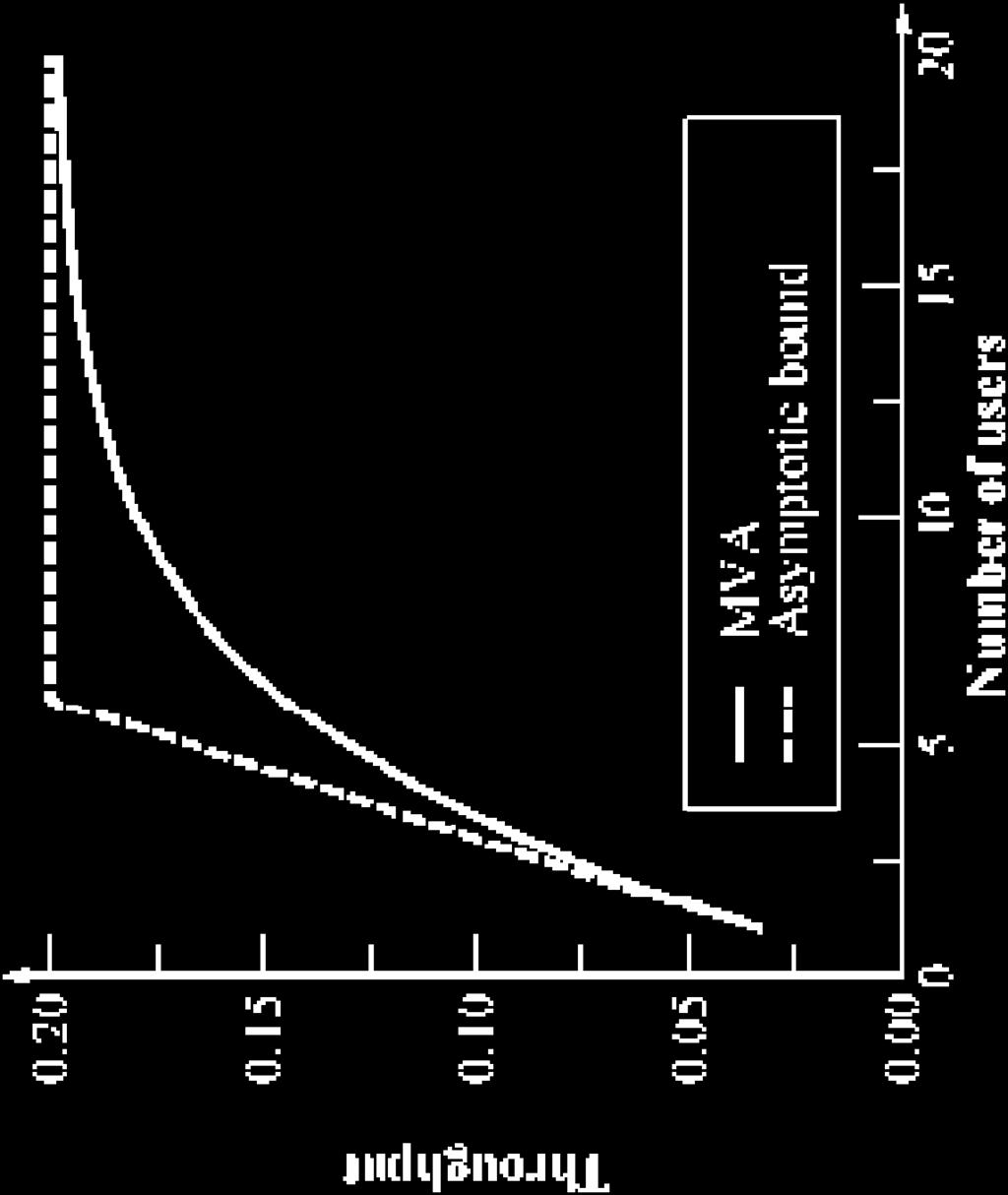
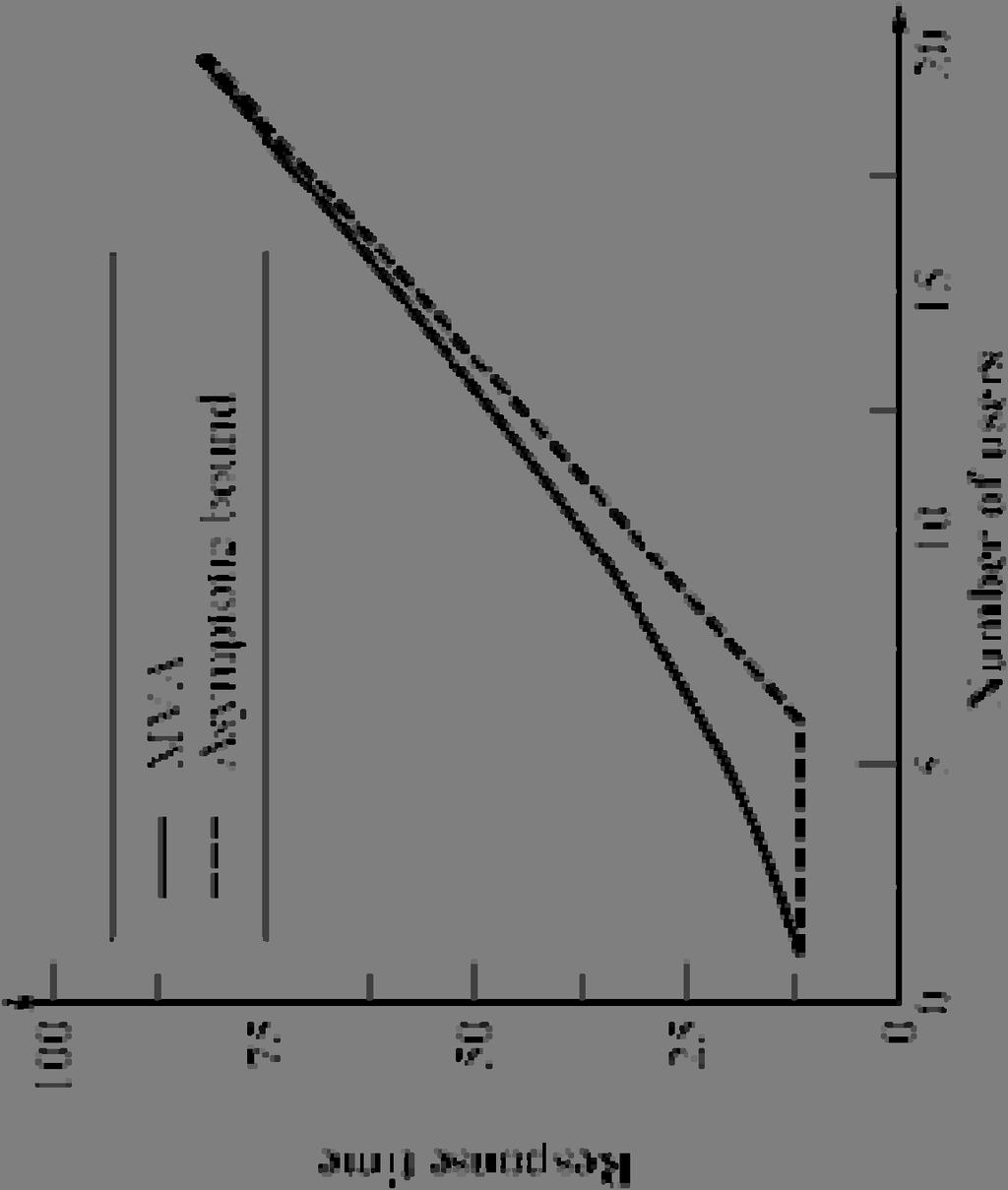
36 Example 33.7: Asymptotic Bounds The knee occurs at: 33-45

37 Quiz 33D The total demands on various devices are as shown. What is the minimum response time? R= D = D CPU + D A + D B = What is the bottleneck device? What is the maximum possible utilization of disk B? U B = What is the maximum possible throughput? X = What is the upper bound on throughput with N users? 1s 5s 0.6s 0.1s A B What is the lower bound on response time with N users? What is the knee capacity of this system? Key: R > max{d, ND max -Z}, X< min{1/d max, N/(D+Z)} 33-46

38 Example 33.8 How many terminals can be supported on 181 =5s the timesharing system of Example 33.2 if the response time has to be kept below 100 seconds? Using the asymptotic bounds on the response time we get: 17 18s 80 50ms A B ms The response time will be more than 100, if: That is, if: the response time is bound to be more than 100. Thus, the system cannot support more than 23 users if a response time of less than 100 is required

39 Quiz 33E For this system, which device would be the bottleneck if: The CPU is replaced by another unit that is twice as fast? Disk A is replaced by another unit that is twice as slow? Disk B is replaced by another unit that is twice as slow? The memory size is reduced so that the jobs make 25 times more visits to disk B due to increased page faults? 1s 5s 0.6s 0.1s A B 33-49

40 Summary Symbols: 33-51

41 Homework 33 Draw a diagram showing the flow of jobs in your system including waiting for disk I/O and network I/O