On Metric and Statistical Properties of Topological Descriptors for geometric Data

Transcription

1 On Metric and Statistical Properties of Topological Descriptors for geometric Data Mathieu Carriere To cite this version: Mathieu Carriere. On Metric and Statistical Properties of Topological Descriptors for geometric Data. Computational Geometry [cs.cg]. Université Paris-Saclay, English. <NNT : 2017SACLS433>. <tel v2> HAL Id: tel Submitted on 30 Jan 2018 HAL is a multi-disciplinary open access archive for the deposit and dissemination of scientific research documents, whether they are published or not. The documents may come from teaching and research institutions in France or abroad, or from public or private research centers. L archive ouverte pluridisciplinaire HAL, est destinée au dépôt et à la diffusion de documents scientifiques de niveau recherche, publiés ou non, émanant des établissements d enseignement et de recherche français ou étrangers, des laboratoires publics ou privés.

2 NNT : 2017SACLS433 Thèse de doctorat de l Université Paris-Saclay préparée à l Université Paris-Sud Ecole doctorale n 580 Sciences et technologies de l information et de la communication Spécialité de doctorat: Informatique par M. Mathieu Carrière On Metric and Statistical Properties of Topological Descriptors for Geometric Data Thèse présentée et soutenue à Paris, le 21 novembre 2017: Composition du Jury : M. Marc Schoenauer, Directeur de recherche INRIA Saclay Président M. Gunnar Carlsson, Professeur émérite Université de Stanford Rapporteur M. Jean-Philippe Vert, Professeur Mines ParisTech Rapporteur M. Julien Mairal, Chargé de recherche INRIA Grenoble Rapporteur M. Ulrich Bauer, Professeur Université technique de Munich Examinateur M. Xavier Goaoc, Professeur Université Paris-Est Examinateur M. Steve Oudot, Chargé de recherche INRIA Saclay Directeur

3 REMERCIEMENTS Tout d abord, j aimerais remercier les personnes qui ont accepté de faire partie de mon jury de thèse : Julien Mairal, Jean-Philippe Vert, Gunnar Carlsson (tous trois ayant de plus rapporté ce manuscrit), Ulrich Bauer, Marc Schoenauer et Xavier Goaoc. Merci aussi à Tamy Boubekeur pour m avoir aidé à organiser la soutenance dans les locaux de Telecom Paris Tech. Ce travail a été financé sur la bourse ERC Gudhi (ERC-2013-ADG ), obtenue par Jean-Daniel Boissonnat, que je remercie également. Bien évidemment, la synthèse de ces trois années de travail au sein de l équipe Geometrica/DataShape (/Tagada?), présentée dans ce document, est moins le fruit d un travail solitaire que de nombreuses collaborations. A ce titre, je souhaite manifester ma gratitude, pour nos discussions toujours enrichissantes, envers mes coauteurs Maks Ovsjanikov, Bertrand Michel, Marco Cuturi, Ulrich Bauer et tout particulièrement mon directeur de thèse Steve Oudot, dont la disponibilité, la patience, la rigueur et les regards profonds (même lors d un footing) sur nos sujets d études ont été des facteurs déterminants pour l épanouissement de ces trois années de travail, et, à titre plus personnel, pour le plaisir que j ai eu à travailler pendant ces trois années à Inria. Ce plaisir est redevable aussi aux membres passés et présents de l équipe (ainsi que des équipes adjacentes). Je remercie Mickaël, Thomas, Amélie, Alice et Etienne, qui m ont chaleureusement accueilli, Eddie, avec qui j ai partagé mon bureau pendant ces trois années, ainsi que les doctorants actuels Dorian, Jérémy, Claire, Nicolas, Théo, Vincent et Raphaël, avec qui j ai passé de très bons moments au dedans et en dehors du labo, et pour qui je souhaite le meilleur pour les années de recherche à venir. Merci aussi à Marc et Fred, et aux postdocs qui se sont succédés pendant ces trois ans, à savoir Hélène, Clément, Ilaria, Pawel et Miro, pour avoir contribué à cette ambiance amicale au travers de nombreuses discussions. Enfin, pour leur soutien administratif exemplaire, merci à Christine et Stéphanie. Les deux mois que j ai passés à Munich dans le groupe Géométrie et Visualisation ont été très enrichissants. Merci à Ulrich Bauer pour avoir permis d organiser ce séjour, ainsi qu aux doctorants du groupe pour le chaleureux accueil et les fréquentes séances de bloc. En dehors du labo, mes amis proches et ma famille ont largement contribué à la qualité de ces trois années. Je souhaite remercier Mathieu, Hugo (Cayla), Hugo (Magaldi), Pauline et Laure, ainsi que tous mes amis parisiens, pour tous les joyeux moments passés ensemble qui ont beaucoup compté pour moi. De même, mes fréquents retours à Toulouse 1

4 ont à chaque fois été grandement revitalisants grâce à Romain, Pierre, Clément et tous mes amis toulousains de longue date, dont l amitié m est très chère. Merci aussi à mes fantastiques colocs Charlotte et Sophie pour tous nos repas et soirées réginaburgiennes que j ai beaucoup appréciées. Je remercie toute ma famille (mes cousins et mes cousines, mes grand parents, oncles et tantes), et plus particulièrement, pour leur soutien et leur affection indéfectibles, je remercie mes parents et mes petits frères, de tout mon coeur. Enfin, merci à toi Aisling, pour tout le temps que nous avons passé ensemble. 2

5 CONTENTS 1 Introduction Introduction en français Analyse de donnée et apprentissage automatique Descripteurs topologiques Principales limitations Contributions Introduction in english Data Analysis and Machine Learning Topological Descriptors Main bottlenecks Contributions Background on Topology Homology Theory Simplices and Simplicial Complexes Simplicial Homology Singular Homology Relative Homology Persistence Theory Filtrations Persistence Modules Persistence Diagram Stability Properties of Persistence Diagrams Extended and Levelset Zigzag Persistence Extended persistence Levelset zigzag persistence Reeb graphs Persistence-based bag-of-features signature Metrics between Reeb graphs Simplification techniques Computation Mapper

6 3 Telescopes and Reeb graphs Telescopes and Operators A lower bound on d b Induced Metrics Conclusion Structure and Stability of the Mapper Mappers for scalar-valued functions MultiNerve Mapper Structure of the MultiNerve Mapper Topological structure of the MultiNerve Mapper A signature for MultiNerve Mapper Induced signature for Mapper Stability in the bottleneck distance Stability with respect to perturbations of the cover Convergence in the functional distortion distance Operators on MultiNerve Mapper Connection between the (MultiNerve) Mapper and the Reeb graph Convergence results An alternative proof of Theorem Conclusion Statistical Analysis and Parameter Selection Approximations of (MultiNerve) Mappers and Reeb graphs Approximation tools Discrete approximations Relationships between the constructions Relationships between the signatures Approximation of a Reeb graph with Mapper Statistical Analysis of the Mapper Statistical Model for the Mapper Reeb graph inference with exact filter Reeb graph inference with estimated filter Confidence sets for the signatures Confidence sets Confidence sets derived from Theorem Bottleneck Bootstrap Numerical experiments Mappers and confidence regions Noisy data Conclusion Kernel Methods for Persistence Diagrams Supervised Machine Learning Empirical Risk Minimization Reproducing Kernel Hilbert Space

7 6.2 A Gaussian Kernel for Persistence Diagrams Wasserstein distance for unnormalized measures on R The Sliced Wasserstein Kernel Metric Preservation Computation Experiments Vectorization of Persistence Diagrams Mapping Persistence Diagrams to Euclidean vectors Stability of the topological vectors Application to 3D shape processing Conclusion Conclusion 177 A Proof of Lemma

8 6

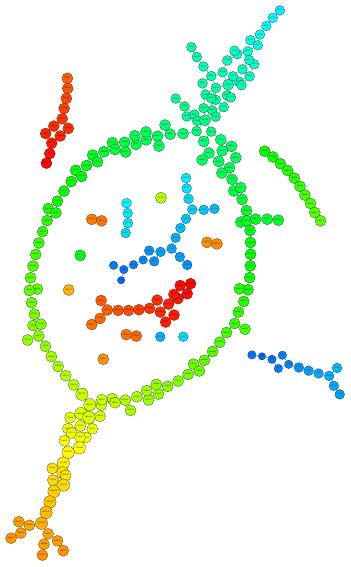
9 LIST OF FIGURES 1.1 Déformations du cercle Ce nuage de points semble échantillonné sur neuf cercle à petite échelle, et sur un seul cercle à plus grande échelle Une base de données d images Diagrames de persistance induit par des boules grossissantes Diagramme de persistance d une image Mapper calculé sur des images Instabilité de Mappers calculés sur des espaces proches Instabilité de Mappers calculés avec des couvertures proches Mapper vu comme une pixelisation du graphe de Reeb Plan de la thèse Deformations of a circle This point cloud seems to be sampled on nine circles from a small scale, and on a single circle from a larger scale A dataset of images Persistence diagrams induced by growing balls Persistence diagram of image Mapper on images Instability of Mapper computed on nearby spaces Instability of Mapper computed with close covers Mapper as a pixelization of the Reeb graph Plan of the thesis Geometric simplices Geometric simplicial complex Boundary operator Cycles Homology of annulus Singular simplex Relative cycle Lower-star filtration Persistence diagram induced by filtration Commutative diagrams for interleaving

10 2.11 Extended filtration Mayer-Vietoris half-pyramid Reeb graph on torus Two Reeb graphs with the same set of features but not the same layout Feature simplification Mapper on double torus Merge Persistence measure for Merge Split Up- and down-forks Shift Persistence measure for Shift Simplification operator Continuous maps Arc number argument Branching argument The space of Reeb graphs is not Cauchy Simplicial poset (MultiNerve) Mapper with bivariate map Left: Staircases of ordinary (light grey) and relative (dark grey) types. Right: Staircases of extended types Q I E is in dark grey while Q I E is the union of Q I E with the light grey area Pyramid rules Zigzag persistence modules in the half-pyramid Mapper as a pixelization of the Reeb graph Stability of the Mapper Full transformation on spaces Full transformation on persistence diagrams Functions on Mapper Interval- and intersection-crossing edges Automatic Mappers on smooth datasets Automatic Mappers on real-world datasets Automatic Mappers on a noisy dataset Kernel trick Concavity argument Orbit recognition Texture and 3D point classification Accuracy and training time dependences on direction number Metric distortion Mapping of a persistence diagram to a sequence with finite support Distances to diagonal Geodesic balls Geodesic balls

11 6.11 MDS on topological vectors knn on topological vectors Stability of topological vectors Symmetry Improvements measured with functional maps Improvements measured directly on shapes A.1 Images of paths in Reeb graph

12 10

13 CHAPTER 1 INTRODUCTION 1.1 Introduction en français Analyse de donnée et apprentissage automatique La génération et l accumulation de données dans des secteurs d activités variés, autant industriels qu académiques, ont pris beaucoup d importance au cours des dernières années, et sont maintenant omniprésents dans de nombreux domaines scientifiques, financiers et industriels. A titre d exemple, en science du numérique, le développement rapide des processus d acquisition et de traitement d images ont permis la mise à disposition publique en ligne d importantes bases de données [93, 89, 107, 112, 123]. De la même manière, en biologie, la nouvelle génération de séquenceurs ont permis à la plupart des laboratoires d aisément déterminer l ADN de différents organismes [14, 78, 88, 100]. Ainsi, la synthétisation et l extraction d informations utiles à partir de ces bases de données massives sont devenus des problèmes d intérêt majeur. L apprentissage automatique est un domaine de la science des données dont le but est de fournir des algorithmes ( automatique ) pouvant réaliser des prédictions sur de nouvelles données à partir seulement de l information déjà présente dans des données préalablement collectées ( apprentissage ). Ces techniques permettent de répondre à de multiples problèmes de l analyse de données, tels que la classification, où l on cherche à prédire des labels, le clustering, où l on cherche à regrouper les données en différents groupes, ou la régression, où l on cherche à approcher une fonction à partir de sa valeur sur les points de données. Nous orientons le lecteur désireux de trouver plus de détails vers [72] pour une introduction complète de ces problématiques. Par exemple, un problème typique de classification est la prédiction de la présence ou non d effets d un médicament sur un patient P. Il s agit d un problème de classification binaire en cela que les labels à prédire sont au nombre de deux, à savoir effet ou sans effet. En supposant qu une base de données est disponible, dans laquelle sont enregistrés les effets ou non du médicament sur plusieurs patients, une des manières les plus simples de procéder est de chercher le patient le plus proche de P dans la base de données, et d attribuer à P le label de ce patient. Cette méthode, simple quoique très efficace, s appelle la prédiction par le plus proche voisin, et a déjà été étudiée en détail. Plus généralement, la prédiction par le plus proche 11

14 voisin n est qu une méthode parmi de nombreuses autres en apprentissage automatique, qui peuvent traiter de problèmes aussi variés que la classification d images, la prédiction du genre musical ou le diagnostic médical, pour ne citer que quelques exemples. D autres exemples d applications sont présentés dans [72]. Descripteurs. En général, les données prennent la forme de nuage de points dans R D, où D N. Chaque point de donnée représente une observation, et chaque dimension, ou coordonnée, représente une mesure. Par exemple, les observations peuvent être des patients, des images ou des séquences d ADN, dont les mesures correspondantes seraient des caractéristiques physiques (la taille, le poids, l âge...), le niveau de gris des pixels, ou des bases azotées A, C, T ou G composant l ADN. Très souvent, le nombre de mesures est élevé, fournissant ainsi beaucoup d informations, mais rendant dans le même temps les données impossibles à visualiser. Ainsi, une grande partie de l analyse de données se consacre à la synthétisation de l information contenue dans les données en des descripteurs simples et interprétables, qui dépendent en général de l application. Par exemple, on peut touver, parmi les descripteurs usuels : le modèle sac-de-mots [130] pour les données textuelles, les descripteurs SIFT [96] et HoG [60] pour les images, la courbure et les images de spin [86] pour les formes 3D, les descripteurs en ondelettes [98] pour le traitement du signal, et, plus généralement, le résultat d une technique de réduction de dimension, comme l ACP, MDS ou Isomap [132]. L efficacité des descripteurs est souvent corrélée aux propriétés dont ils bénéficient. En fonction de l application, il peut être pertinent d exiger d un descripteur qu il soit invariant par translation ou rotation, intrinsèque ou extrinsèque, un vecteur Euclidien, etc. Trouver des descripteurs avec de telles propriétés est une question importante car permettant d améliorer grandement l interprétation et la visualisation des données, comme mentionné plus haut, mais aussi le résultat des algorithmes d apprentissage, qui sont susceptibles de produire de mauvaises performances si alimentés avec des données brutes. Le but de cette thèse est d étudier une classe spécifique de descripteurs appelés topologiques, et qui sont connus pour être invariants aux déformations continues des données qui n impliquent pas de déchirement ou de recollement [26] Descripteurs topologiques L idée derrière les descripteurs topologiques est de synthétiser l information topologique présente dans les données [26]. Intuitivement, la topologie des données englobe toutes les propriétés qui sont préservées par des déformations continues, comme l étirement, le rétrécissement ou l épaississement, sans déchirure ni recollement. Par exemple, si un cercle est continument déformé sans déchirement ou recollement, un trou va toujours subsister dans l objet résultant, quelle qu ait été la transformation. C est ce qu on appelle un attribut topologique. Voir la Figure 1.1, où la présence d un trou est attestée dans différentes déformations du cercle. De manière similaire, les composantes connexes, cavités, et trous de dimension supérieure sont des attributs topologiques. Dans l optique de formaliser la présence de tels attributs (en toute dimension), la théorie de l homologie, a été développée au 19e et au début du 20e siècle. Elle se présente comme un encodage algébrique de l information topologique. L homologie d un espace est une famille de groupes abéliens (un pour chaque dimension), 12

15 Figure 1.1: Déformations du cercle. Figure 1.2: Ce nuage de points semble échantillonné sur neuf cercle à petite échelle, et sur un seul cercle à plus grande échelle. dont les éléments sont des combinaisons linéaires des trous de l espace. Cependant, les groupes d homologie ne sont pas des descripteurs topologiques très performants en tant que tels, la raison principale étant que les données prennent souvent la forme de nuages de points, dont les groupes d homologie ne sont pas informatifs : chaque point du nuage est un générateur du groupe d homologie en dimension 0, puisque l homologie en dimension 0 compte les composantes connexes, et tous les groupes d homologie de dimension supérieure sont triviaux puisque le nuage n a aucun trou. Evidemment, le nuage de points peut tout de même refléter de l information topologique - par exemple s il est échantillonné sur un objet géométrique comme un cercle, une sphère ou un tore. La question devient ainsi celle de l échelle avec laquelle observer les données, comme illustré dans la Figure 1.2. L analyse de données topologiques fournit deux constructions : les diagramme de persistance, qui synthétisent l information topologique à toutes les échelles, et les Mappers, qui encodent plus d information géométrique à échelle fixée. Diagrammes de persistance. Puisque chaque échelle fournit des informations topologiques pertinentes, l idée de l homologie persistante est d encoder l homologie du nuage de points à toutes les échelles. Considérons la base de données de la Figure 1.3, contenant des images à pixels, vus comme des vecteurs en dimension , où chaque coordonnée est le niveau de gris d un pixel. Puisque la caméra a tourné autour de l objet, il s ensuit qu à petite échelle, les données semblent être réparties en petits groupes, tandis qu à échelle plus grande, elles semblent échantillonnées sur un cercle (plongé dans R ). Figure 1.3: Une base de données d images. Pour synthétiser cette information, on peut faire grossir des boules centrées sur les points de données. Considérons trois rayons différents pour ces boules : un petit α, un légèrement plus grand β et un beaucoup plus grand γ, comme montré dans la Figure 1.4. Quand le rayon des boules vaut α, l union des boules est simplement l union de dix composantes connexes, dont l homologie en dimension 1 et supérieure est triviale. Cependant, quand le rayon devient β, l union des boules a l homologie d un cercle, dont le trou en dimension 1 devient rempli quand le rayon devient γ. On dit que les composantes 13

16 r = α r = β r = γ γ β α α β γ Figure 1.4: Trois différentes unions de boules centrées sur des images vus comme des vecteurs dans un espace Euclidien de grande dimension. L apparition et la disparition d attributs topologiques, comme des composantes connexes ou des trous, est enregistrée dans un diagramme de persistance, dans lequel les points représentant des attributs en dimension 0 sont en vert, et ceux représentant des attributs en dimension 1 sont en violet. connexes sont nées à la valeur α, et neuf sont mortes, c est-à-dire se sont fait relier à la dixième, à la valeur β. De la même manière, le trou en dimension 1 est apparu au rayon β, et a disparu au rayon γ. Enfin, la dixième composante connexe est apparue au rayon α et a persisté jusqu au rayon γ. Cette information est encodée dans le diagramme de persistance, qui est un multi-ensemble 1 de points, chacun représentant un attribut topologique, et ayant les rayons de naissance et de mort comme coordonnées. La distance à la diagonale fournit une quantité utile et interprétable dans les diagrammes de persistance. En effet, si un point est loin de la diagonale, alors son ordonnée est largement supérieur à son abscisse, ce qui signifie que l attribut topologique correspondant était présent dans l union des boules pour une large gamme de rayons différents, indiquant ainsi que l attribut topologique a des chances d être présent dans l objet sous-jacent, et d être une information pertinente. Au contraire, les points proches de la diagonale représentent des attributs qui ont disparu rapidement après être apparus. Ces attributs éphemères correspondent plutôt à du bruit ou des attributs de l objet sous-jacent qui ne sont pas pertinents. C est le cas par exemple des neuf composantes connexes de l union des boules au rayon α dans la Figure 1.4, qui ont disparu au rayon β, proche de α. Il est à noter que nous avons éxpliqué la construction dans le cas où il n y a que trois unions 1 Un multi-ensemble est une généralisation d un ensemble, dans laquelle les points ont des multiplicités. 14

17 de boules, mais il est bien sûr possible de construire un diagramme de persistance quand le rayon des boules augmente continument de 0 à +. Dans ce cas, le trou de dimension 1 a une abscisse située entre α et β (car il n est pas encore présent pour le rayon α et est déjà là au rayon β), et une ordonnée située entre β et γ (car il a déjà disparu au rayon γ). De même, toutes les composantes connexes ont pour abscisse 0. Neuf d entre elles 2 ont une ordonnée comprise entre α et β et l ordonnée de la dixième est + puisqu elle est toujours présente, quelque soit le rayon des boules. Les diagrammes de persistance peuvent en faire être définis beaucoup plus généralement. - même si l interprétation en terme d échelle n est plus forcément pertinente. Tout ce qui est requis est une famille d espaces intriqués les uns dans les autres, appelée filtration, c est-à-dire une famille {X α } α A, où A est un ensemble d indices totalement ordonnés, telle que α β X α X β. La construction du diagramme de persistance est alors la même, c est-à-dire l enregistrement de l apparition et de la disparition d attributs topologiques quand on parcourt A par ordre croissant. Dans l exemple précédent, la filtration contient trois espaces, qui sont les trois différentes unions de boules, chaque union étant indicée par le rayon de ses boules. Il est clair dans ce cas que ces trois espaces sont intriqués car une boule est toujours incluse dans la boule de même centre avec un rayon supérieur. Une manière pratique de construire une filtration est d utiliser les sous-niveaux d une fonction continue à valeurs réelles f, c est-à-dire les espaces de la forme f 1 ((, α]). En effet, il est évident que f 1 ((, α]) f 1 ((, β]) pour tous α β R. Par exemple, l union des boules de rayon r centrées sur les points d un nuage P est égale au sous-niveau de la fontion distance au nuage P : d 1 P ((, r]), où d P (x) = min p P d(x, p). Ainsi, dès qu une fonction continue à valeurs réelles est à disposition, un diagramme de persistance peut être construit, ce qui explique pourquoi le diagramme de persistance est un descripteur prolifique. Prenons par exemple l image floue d un zéro, affichée dans le coin inférieur droit de la Figure 1.5, pour laquelle le niveau de gris des pixels est utilisé comme fonction continue pour calculer un diagramme de persistance. De nouveau, on trouve deux points se distinguant des autres dans le diagramme de persistance, l un représentant la composant connexe du zéro, et l autre son trou de dimension 1. Le reste des points est engendré par le bruit présent dans l image. Une des raisons pour lesquelles les diagrammes de persistance sont des descripteurs appréciés est qu en plus d être invariant par déformation continue (sans déchirement ou recollement), ils sont stables [42, 54]. En effet, si des diagrammes de persistance sont calculés avec les sous-niveaux de fonctions similaires, alors la distance entre eux est bornée supérieurement par la différence entre les fonctions en norme infinie : d b (Dg(f), Dg(g)) f g, où d b désigne la distance bottleneck entre diagrammes de persistance, qui est le coût de la meilleure correspondance partielle entre les points de chaque diagramme. Cela signifie que, par exemple, si les positions des images de la Figure 1.4 sont légèrement perturbées, ou si l image floue du zéro de la Figure 1.5 est légèrement modifiée, les diagrammes de persistance correspondant seront très proches des originaux avec la distance bottleneck. Les diagrammes de persistance ont aidé à améliorer l analyse des données dans de 2 En fait, chaque point est une composante connexe au rayon 0. 15

18 f f f f Figure 1.5: Autre exemple d une construction de diagramme de persistance, avec les sous-niveaux du niveau de gris des pixels d une image floue d un zéro. nombreuses applications, allant de l analyse de forme 3D [38, 43] à la transition de phase de matériaux [73, 84] et la génomique [24, 39] pour n en citer que quelques-unes. Mapper. Comme expliqué plus haut, les diagrammes de persistance synthétisent l information de nature topologique contenue dans les données. Cependant, ils perdent beaucoup d information géométrique dans le processus : ils est aisé de construire des espaces différents ayant les mêmes diagrammes de persistance. Le Mapper 3, introduit par [129], est une approximation directe de l objet sous-jacent, qui contient non seulement les attributs topologiques, mais aussi de l information additionnelle, concernant le positionnement des attributs les uns par rapport aux autres par exemple. Comme pour les diagrammes de persistance, une fonction réelle continue, appelée parfois filtre, est requise, ainsi qu une couverture de son image par des intervalles ouverts qui se chevauchent. L idée est de calculer les antécédents par f de tous les intervalles de la couverture, de les raffiner en leurs composantes connexes via des techniques de clustering, et de finalement lier les composantes connexes entre elles si elles contiennent des points de données en commun. Nous fournissons un exemple dans la Figure 1.6, où nous considérons de nouveau le nuage d images. La fonction réelle continue est la valeur absolue de l angle à partir duquel l image a été prise, et son image [0, π] est couverte par trois intervalles (bleu, rouge et vert). Dans les antécédents des intervalles rouge et bleu, il y a une seule composant 3 Dans cette thèse, on appelle Mapper l objet mathématique, et pas l algorithme utilisé pour le construire. 16

19 π 0 Figure 1.6: Exemple de Mapper calculé sur le nuage d images, avec la fonction d angle et une couverture de trois intervalles. connexe, tandis qu il y en a deux dans l antécédent de l intervalle vert. Le Mapper est obtenu en ajoutant des arètes entre les composantes connexes, en fonction de la présence ou non de points de données en commun à l intérieur de ces composantes; par exemple, les composantes connexes vertes et bleues, ou vertes et rouges, sont reliées, mais pas celles qui sont rouges et bleues. Le Mapper a l homologie d un cercle, est constitue une approximation directe du support sous-jacent au nuage d images. Il est bon de remarquer que les longueurs des intervalles contrôlent directement l échelle à partir de laquelle on observe le nuage : si les intervalles sont petits, le Mapper va avoir beaucoup de composantes déconnectées puisque les antécédents contiendront au plus un point de donnée. A l opposé, si les intervalles sont larges, le Mapper aura peu de composantes puisque les antécédents vont contenir beaucoup de points de données. En pratique, le Mapper a deux domaines d applications majeures. Le premier est la visualisation et le clustering. En effet, le Mapper fournit une visualisation des données sous forme de graphe dont la topologie reflète celle des données. Il apporte ainsi une information complémentaire à celle des algorithmes de clustering usuels concernant la structure interne des clusters par l identification de branches et de boucles qui mettent en lumière des attributs topologiques potentiellement remarquables dans les groupes identifiés par clustering. Voir par exemple [138, 97, 125, 83] pour des exemples d applications. La deuxième application est la sélection d attributs. En effet, chaque attribut des données peut être évalué en regard de sa capacité à différencier les attributs topologiques mentionnés plus haut (branches et boucles) du reste des données, via l utilisation de tests statistiques, comme celui de Kolmogorov-Smirnov. Voir par exemple [97, 109, 122] pour des exemples d applications Principales limitations Même si le Mapper et les diagrammes de persistance bénéficient de propriétés désirables, plusieurs limitations refrènent leur usage pratique, à savoir la la difficulté de la sélection de paramètres pour Mapper et la non linéarité de l espace des diagrammes de persistance. 17

20 Distance et stabilité pour les Mappers et les graphes de Reeb Un problème du Mapper est que, contrairement aux diagrammes de persistance, il a un paramètre, la couverture, dont la sélection à priori est difficile. A cause de cela, le Mapper apparaît comme une construction très instable : il arrive que des Mappers calculés sur des nuages de points similaires, comme dans la Figure 1.7, ou avec des couvertures proches, comme dans la Figure 1.8, soient très différents. Figure 1.7: Mappers calculés sur des échantillonnages similaires du cercle, avec la fonction hauteur et une couverture composée de trois intervalles. Ce problème majeur est un obstacle important à son utilisation en exploration de données. La seule réponse dans l état-de-l art consiste à sélectionner des paramètres dans une grille de valeurs pour lesquels le Mapper semble stable - voir [109] par exemple. Ainsi, prouver un résultat de stabilité pour les Mappers nécessite de les comparer avec une distance qui dépend au moins de la couverture utilisée. Malheureusement, même si des distances théoriques peuvent être définies [105], la définition d une distance calculable et interprétable entre Mappers manque dans l état-de-l art. Pour gérer ce problème, on peut prendre inspiration d une classe de descripteurs très semblables aux Mappers, les graphes de Reeb. Graphes de Reeb. Même si les Mappers sont définis pour des nuages de points, leur extension à des espaces non discrets est évidente, la différence étant que des techniques de clustering ne sont pas nécessaires pour calculer les composantes connexes des antécédents puisqu elles sont bien définies. Dans ce cas, faire tendre la longueur des intervalles vers zéro définit le graphe de Reeb. Ainsi, les Mappers (calculés sur des espaces non discrets) ne sont que des approximations, ou des versions pixelisées des graphes de Reeb, comme illustré dans la Figure 1.9. Cette observation est cruciale car plusieurs distances, ainsi que des résultats de stabilité, ont été obtenus pour les graphes de Reeb [7, 8, 61] et peuvent être étendus aux Mappers. Cependant, ces distances ne sont pas calculables et ne peuvent pas être utilisées en tant que telles en pratique [2]. La question de savoir s il est possible de définir des distances stables et calculables pour les Mappers reste ainsi ouverte. Non linéarité de l espace des diagrammes de persistance. Même si les diagrammes de persistance sont stables, ils ne peuvent pas être utilisés systématiquement 18

21 g /r Figure 1.8: Un ensemble de Mappers calcule s sur le jeu de donne es du crate re avec des couvertures diffe rentes (r est la longueur des intervalles et g est le pourcentage de chevauchement) et la coordonne e horizontale. Gauche : jeu de donne es du crate re colore par les valeurs de fonction, allant de bleu a orange. Droite : Mappers calcule s avec des parame tres diffe rents. Les rectangles violets indiquent les attributs topologiques qui apparaissent ou disparaissent soudainement dans les Mappers. Figure 1.9: Une surface plonge e dans R3 (gauche), son graphe de Reeb calcule avec la fonction hauteur (milieu) et son Mapper calcule avec la fonction hauteur et une couverture a deux intervalles (droite). par des algorithmes d apprentissage automatique. En effet, une classe tre s large de ces algorithmes ne cessitent que les donne es soient soit des vecteurs d un espace Euclidien (comme les fore ts ale atoires), ou d un espace de Hilbert (comme les SVM). L espace des diagrammes de persistance, e quipe avec la distance bottleneck, n est malheureusement ni l un ni l autre. Me me les moyennes de Fre chet ne sont pas bien de finies [136]. L astuce du noyau permet cependant de traiter ce genre de donne es. En supposant que les points de donne es vivent dans un espace me trique (X, dx ), l astuce du noyau ne cessite seulement une fonction semi-de finie positive, appele e noyau, c est-a -dire une fonction k : X X R telle que, pour tous a1,, an R et x1,, xn X, on ait : X ai aj k(xi, xj ) 0. i,j Gra ce au the ore me de Moore-Aronszajn [4], les valeurs du noyau calcule es sur des points de donne es peuvent e tre de montre es e gales a l e valuation d un produit scalaire entre les 19

22 images des points de données par un plongement dans un espace de Hilbert spécifique qui dépend uniquement de k et qui est en général inconnu. Plus formellement, il existe un espace de Hilbert H k tel que, pour tous x, y X, on ait : k(x, y) = Φ k (x), Φ k (y) Hk, pour un certain plongement Φ k. Les valeurs du noyau peuvent donc être considérées comme des produits scalaires généralisés entre les points de données, et peuvent être directement utilisés par les algorithmes d apprentissage. Dans le cas qui nous intéresse, la question est ainsi de trouver de tels noyaux pour les diagrammes de persistance. Une manière standard de procéder pour définir un noyau pour des points d un espace métrique (X, d X ) est d utiliser des fonctions Gaussiennes : ( k σ (x, y) = exp d ) X(x, y), 2σ 2 où σ > 0 est un paramètre d échelle. Un théorême de Berg et al. [11] stipule que k σ est un noyau, c est-à-dire une fonction semi-définie positive, pour tous σ > 0 si et seulement si d X est conditionnellement semi-définite négative, c est-à-dire est telle qu on ait i,j a ia j d X (x i, x j ) 0 pour tous x 1,, x n X et a 1,, a n R tels que n i=1 a i = 0. Malheureusement, comme montré par Reininghaus et al. [119], la distance bottleneck d b pour les diagrammes de persistance n est pas conditionnellement semi-définite négative. Il est même possible de trouver des contre-exemples pour les distances de Wasserstein, une autre classe de distance pour diagrammes. L utilisation de noyaux Gaussiens pour les diagrammes de persistance est donc impossible avec leurs métriques canoniques. Néanmoins, plusieurs noyaux ont été proposés au cours des dernières années [1, 20, 90, 120], bénéficiant tous de résultats de stabilité bornant supérieurement la distance entre les plongements des diagrammes par les distances bottleneck ou de Wasserstein entre les diagrammes eux-mêmes. En d autres termes, la distorsion métrique dist(dg, Dg ) = Φ k(dg) Φ k (Dg ) Hk d b (Dg, Dg ) est bornée supérieurement. Cependant, le calcul d une borne inférieure non triviale reste ouvert : il se pourrait que les plongements de diagrammes différents soient en fait très proches l un de l autre, ce qui n est pas désirable en pratique pour la discriminativité d un noyau. Par exemple, le plongement constant, qui envoie tous les diagrammes sur un même point d un espace de Hilbert spécifique, est stable (les distances entre images dans l espace de Hilbertétant toujours nulles), mais les résultats du noyau correspondant seront évidemment très faibles. Plus généralement, le comportement et les propriétés des distances dans les espaces de Hilbert induits par des noyaux sont flous, et la question de savoir s il existe des noyaux avec des propriétés théoriques de discriminativité est ouverte Contributions Dans cette thèse, nous nous penchons sur trois problèmes : l interprétation des attributs topologiques) du Mapper (par exemple avec des régions de confiance), le réglage de ses paramètres, et l intégration globale des descripteurs topologiques en apprentissage automatique. 20

23 Distance entre graphes de Reeb. Dans le Chapitre 3, nous définissons une pseudodistance calculable entre graphes de Reeb, qui revient à comparer leurs diagrammes de persistance. Nous montrons aussi que cette pseudodistance est en fait localement équivalente aux autres distances existantes pour les graphes de Reeb. Cette équivalence locale est alors utilisée pour étudier les propriétés de l espace métrique des graphes de Reeb, équipé des distances intrinsèques. Nous montrons que toutes ces distances intrinsèques sont fortement équivalentes, ce qui nous permet d englober toutes les techniques pour comparer des graphes de Reeb en une seule approche. Ce travail a été publié dans les proceedings du Symposium on Computational Geometry 2017 [36]. Structure du Mapper. Dans le Chapitre 4, nous fournissons un lien entre les diagrammes de persistance du graphe de Reeb et ceux du Mapper (calculé sur le même espace topologique). Plus spécifiquement, nous montrons que le diagramme de persistance du Mapper est obtenu à partir de celui du graphe de Reeb en supprimant des points spécifiques, à savoir ceux qui appartiennent à des régions du plan qui dépendent uniquement de la couverture utilisée pour calculer le Mapper. Cette relation explicite nous permet alors d étendre la pseudodistance entre graphes de Reeb aux Mappers. Nous montrons finalement que cette pseudodistance stabilise les Mappers : nous fournissons un théorême de stabilité pour des Mappers comparés avec cette pseudodistance. Ce travail a été publié dans les proceedings du Symposium on Computational Geometry 2016 [35] et une version longue a été soumise au Journal of Foundations of Computational Mathematics [34]. Cas discret. Dans le Chapitre 5, nous étendons les résultats précédents au cas où les Mappers sont calculés sur des espaces discrets, c est-à-dire des nuages de points, et les composantes connexes sont calculées avec du single-linkage clustering. En particulier, nous fournissons des conditions suffisantes pour lesquelles le Mapper calculé sur un nuage de points coincide avec celui calculé sur le support. De plus, nous montrons que le Mapper converge vers le graphe de Reeb avec une vitesse de convergence optimale, au sens où aucun estimateur du graphe de Reeb ne peut converger plus vite. Les paramètres utilisés pour démontrer l optimalité fournissent en plus des heuristiques pour le réglage automatique de ces paramètres. Ces heuristiques se basent sur des techniques de sous-échantillonnage et dépendent uniquement de la cardinalité du nuage de points de données. Finalement, nous proposons un moyen de calculer des régions de confiance pour les différents attributs topologiques du Mapper. Ce travail a été soumis au Journal of Machine Learning Research [33]. Méthodes à noyaux. Dans le Chapitre 6, nous appliquons des techniques d apprentissage aux diagrammes de persistance, via des méthodes à noyaux. Nous définissons d abord un noyau Gaussien en utilisant une modification de la distance de Wasserstein, appelée distance de Sliced Wasserstein. Nous montrons en effet que cette distance, à l inverse de la distance de Wasserstein, est bien conditionnellement semi-définie négative, et permet donc de définir un noyau Gaussien. De plus, nous montrons que la distance induite dans l espace de Hilbert associé est équivalente à la distance de Wasserstein de départ. Ainsi, ce noyau, en plus d être stable et Gaussien, est aussi théoriquement discriminant. Nous en fournissons aussi une preuve empirique en obtenant 21

24 de nettes améliorations par rapport aux autres noyaux de l état-de-l art dans plusieurs applications. Ce travail a été publié dans les proceedings de l International Conference on Machine Learning 2017 [32]. Enfin, nous définissons aussi une méthode de vectorisation pour envoyer les diagrammes de persistance dans R D, où D N. Ce plongement stable, même si non injectif, permet l usage des diagrammes de persistance pour des problèmes et algorithmes où des vecteurs Euclidiens sont nécessaires. Nous détaillons alors une application où une telle structure est requise, à savoir le traitement de formes 3D, pour laquelle nous démontrons que les diagrammes de persistance apportent une information complémentaire aux descripteurs traditionnels. Ce travail a été publié dans les proceedings du Symposium on Geometry Processing 2015 [38]. Comment lire cette thèse? Cette thèse est composée de quatre parties différentes : La première est le Chapitre 2, dans lequel nous détaillons les fondations théoriques de l homologie, la persistance, les graphes de Reeb et les Mappers. Nous expliquons aussi la persistance étendue et la persistance en zigzag. La deuxième partie est le Chapitre 3, qui traite des graphes de Reeb et de leurs distances. La troisième partie est composée des Chapitres 4 et 5, qui traitent de Mapper. La quatrième partie est le Chapitre 6. Il traite des noyaux pour les diagrammes de persistance, dans des espaces de Hilbert en dimension finie et infinie. Voir la Figure Le Chapitre 2 rappelle essentiellement les fondamentaux en topologie. Les autres chapitres contiennent en revanche les contributions de cette thèse. Les Chapitres 3 et 4 sont très orientés topologie, tandis que le Chapitre 5 utilise plutôt des notions de statistiques, et que le Chapitre 6 se concentre davantage sur l apprentissage automatique. Ces chapitres ne sont pas indépendants, comme illustré par la Figure 1.10, mais les contributions de chaque chapitre sont énoncées dans les introductions correspondantes. Ainsi, pour chacun de ces chapitres, le lecteur, en fonction de ses goûts ou connaissances personnelles, peut soit se limiter à l introduction, soit lire le chapitre dans son intégralité. 22

25 Kernel Methods Chapter Mapper 2.4 Reeb graphs 2.3 Extended/Zigzag 2.2 Persistence 2.1 Homology Background Chapter 2 2.1, , 2.2, 2.3, 2.4, , 2.2, 2.3, 2.4 Mapper Chapter 5 Chapter 4 Reeb graph 3.1 Chapter 3 Figure 1.10: Les flèches indiquent des dépendances entre chapitres, et les flèches en pointillés indiquent des dépendances partielles, c est-à-dire que seule une petite et non essentielle partie du chapitre dépend de l autre. 23

26 1.2 Introduction in english Data Analysis and Machine Learning Data collection and generation in various human activities, including both industry and academia, have grown exponentially over the last decade and are now ubiquitous in many different fields of science, finance and industry. For example, in digital science, the fast development of image acquisition and processing has allowed large amounts of images to become publicly available online [93, 89, 107, 112, 123]. Similarly, in biology, next generation high-throughput sequencing allowed most laboratories to easily determine DNA sequences of sample organisms [14, 78, 88, 100]. Hence, the need to summarize and extract useful information from these massive amounts of data has become a problem of primary interest. Machine Learning is a field of data science that aims at deriving algorithms ( Machine ) that can make predictions about new data solely from the information that is contained in already collected datasets ( Learning ). These techniques can provide answers to multiple data analysis problems such as classification, which aims at predicting labels, clustering, which aims at separating data into groups or clusters, or regression, which aims at approximating functions on data. We refer the interested reader to [72] for a comprehensive introduction to these methods. For example, a typical classification problem would be to predict if a drug have effects on a specific patient P. This is a binary classification problem since the label we want to predict for P is either effect or no effects. Assuming you have a database of patients at hand, in which the drug effects on each patient were recorded, one of the simplest way to proceed is to look for the closest match, or most similar patient, to P in this database, and to take the label of this match. This extremely simple yet powerful method is called nearest neighbor prediction, and has been extensively studied by data scientists. More generally, nearest neighbor prediction is nothing but a small part of the large variety of methods proposed in Machine Learning, which can tackle many real-life challenges including image classification, musical genre prediction or medical prognosis to name a few. More examples of applications and datasets can be found in [72]. Descriptors. Usually, data comes in the form of a point cloud in R D, where D N. Each data point represents an observation and each dimension, or coordinate, represents a measurement. For instance, observations can be patients, images or DNA sequences, whose corresponding measurements are physical characteristics (height, weight, age...), grey scale values of pixels or nucleobases A,C,T,G composing DNA. It is often the case that the number of measurements is very large, leading to a rich level of information, but also making data very high-dimensional and impossible to visualize. Hence, a large part of data analysis is devoted to the summarization of the information contained in datasets or data points into simple and interpretable descriptors or signatures, which are usually application specific. For instance, among common descriptors are: bag-of-words models [130] for text document data, SIFT [96] and HoG [60] descriptors for image data, curvature and spin images [86] for 3D shape data, wavelet descriptors [98] for signal data, and, more generally, outputs of data reduction technique, such as MDS, PCA or Isomap [132]. The efficiency of descriptors is very often correlated 24

27 Figure 1.11: Deformations of a circle. Figure 1.12: This point cloud seems to be sampled on nine circles from a small scale, and on a single circle from a larger scale. to the properties they enjoy. Depending on the application, one may want descriptors to be translation or rotation invariant, intrinsic or extrinsic, to lie in Euclidean space, etc. Deriving descriptors with desirable properties is important since it greatly enhances interpretation and visualization, as mentioned above, but it also improves the performances of Machine Learning algorithms, which may perform poorly if fed with raw data. The aim of this thesis is to study a specific class of descriptors called topological descriptors, which are known to be invariant to continuous deformations of data that do not involve tearing or gluing [26] Topological Descriptors The idea of topological descriptors is to summarize the topological information contained in data [26]. Intuitively, the topology of data encompasses all of its properties that are preserved under continuous deformations, such as stretching, shrinking or thickening, without tearing or gluing. For instance, when a circle is continuously deformed without tearing or gluing, the hole always remains in the resulting object, whatever the transformation. This is a topological invariant or feature. See Figure 1.11, where a hole is always present in the displayed deformations of the circle. Similarly, connected components, cavities and higher-dimensional holes are topological features. In order to formalize the presence of such holes (in any dimension), homology theory was developed in the 19th and the beginning of the 20th century. It provides an algebraic encoding of such topological information. Basically, the homology of a space is a family of abelian groups (one for each topological dimension), whose elements are linear combinations of the space s holes. However, it turns out that the homology groups themselves perform poorly as topological descriptors. The main reason is that data often comes in the form of point clouds, and the homology groups are not informative for such objects: each point of the cloud is a generator of the 0-dimensional homology group, since 0-dimensional homology is concerned with connected components, and all higher-dimensional homology groups are trivial since the point cloud has no holes. However, it may happen that the data still contains topological information, for instance when the point cloud is a sampling of a geometric object such as a circle, a sphere or a torus. Hence, the question that arises is that of the scale at which one should look at the data, as illustrated in Figure Topological data analysis provides two constructions: persistence diagrams, which summarize the topological information at all possible scales, and Mappers, which encode extra geometric information but at a fixed scale. 25

28 Persistence diagrams. Since several different scales may contain relevant topological information, the idea of persistent homology is to encode the homology of the point cloud at all possible scales. Consider the dataset of Figure 1.13, containing images with pixels, seen as 16,384-dimensional vectors, where each coordinate is the grey scale value of a pixel. Since the camera circled around the object, it follows that, from a small scale, the data looks composed of small clusters, each of which characterizing a specific angle, whereas from a larger scale, the data seems to be sampled on a circle (embedded in R 16,384 ). Figure 1.13: A dataset of images. To summarize this information, the idea is to grow balls centered on each point of the dataset. Let us look at three different radius values: a small one α, a slightly larger intermediate one β, and a very large one γ for these balls, as displayed in Figure r = α r = β r = γ γ β α α β γ Figure 1.14: Three different unions of balls centered on images seen as vectors in high-dimensional Euclidean space. The appearance and disappearance of topological features like connected components or holes is recorded and stored in the so-called persistence diagram, in which green points represent 0-dimensional features and purple points represent 1-dimensional features. When the radius of the balls is α, the union of balls is a just a union of ten connected components with trivial homology in dimension 1 and above. However, when the radius is 26

29 β, the union of balls has the homology of a circle, whose 1-dimensional hole gets filled in when the radius increases to γ. Hence, we say that the connected components were born at value α, and nine of them died, or got merged in the tenth one, at radius β. Similarly, the 1-dimensional circle was born, or appeared, at value β and died, or got filled in, at value γ. Finally, the tenth connected component appeared at radius α and remained all the way until radius γ. This is summarized in the persistence diagram, which is a multiset 4 of points, each of which represents a topological feature and has the birth and death radii as coordinates. The distance to the diagonal is a useful interpretable quantity in persistence diagrams. Indeed, if a point is far from the diagonal, then its ordinate, or death radius, is much larger than its abscissae, or birth radius. This means that the corresponding topological feature was present in the union of balls for a large interval of radii, suggesting that the feature is likely to be present in the underlying object, and thus significant. On the contrary, points close to the diagonal represent features that disappeared quickly after their appearance. These fleeting features are likely to be nonsignificant features or noise artifacts. Consider for instance the nine connected components in the union of balls of radius α in Figure 1.14, which disappeared at radius β slightly larger than α. Note that we explained the construction using only three unions of balls, but it is of course possible to compute a persistence diagram when the radius increases continuously from 0 to +. In that case, the 1-dimensional hole has an abscissa located between α and β (since it is not yet present at radius α and already present at radius β), and an ordinate located between β and γ (since it is already gone at radius γ). Similarly, all connected components have an abscissa equal to 0. Nine of them 5 have an ordinate located between α and β and the ordinate of the tenth one is + since it is always present, whatever the radius of the balls. Persistence diagrams can actually be defined much more generally even though the interpretation with scales may no longer be true. All that is needed is a family of spaces which is nested with respect to the inclusion, called a filtration. This is a family {X α } α A, where A is a totally ordered index set, such that α β X α X β. Then, the construction of persistence diagrams remains the same, i.e. keeping track of the appearance and disappearance of topological features as we go through all indices in ascending order. In the previous example, the filtration had three elements, the three different unions of balls, each union being indexed by the radius of its balls. It is clear in this case that these three spaces are nested since a ball is always included in the ball with same center and larger radius. A common way to build a filtration is to use the sublevel sets of a continuous scalarvalued function f, which are sets of the form f 1 ((, α]). Indeed, it is clear that f 1 ((, α]) f 1 ((, β]) for any α β R. For instance, the union of balls with radius r centered on the points of a point cloud P is equal to the sublevel set of the distance function to P : d 1 P ((, r]), where d P (x) = min p P d(x, p). Hence, as soon as there is a continuous scalar-valued function at hand, a persistence diagram can be computed, which explains why the persistence diagram is a versatile descriptor. Consider for instance the blurry image of a zero in the down right corner of Figure 1.15, where the grey value function is used to compute the persistence diagram. Again, there are two points standing out in the persistence diagram, one representing the connected 4 A multiset is a generalization of a set, in which points can have multiplicities. 5 Actually, each point is a connected component at radius 0. 27

30 component of the zero, and the other representing the 1-dimensional hole induced by the zero. All other points are noise. f f f f Figure 1.15: Another example of a persistence diagram construction with the sublevel sets of the grey value function defined on a blurry image of a zero. One of the reasons why persistence diagrams are useful descriptors is that, in addition to be invariant to continuous deformations (that do not involve tearing or gluing), they are stable [42, 54]. Indeed, if persistence diagrams are computed with sublevel sets of similar functions, then the distance between them is upper bounded by the difference between the functions in the sup norm: d b (Dg(f), Dg(g)) f g, where d b stands for the bottleneck distance between persistence diagrams, which is the cost of the best partial matching that one can find between the points of the persistence diagrams. This means that, for instance, if the positions of the images in Figure 1.14 are slightly perturbed, or if the blurry image of a zero in Figure 1.15 is slightly changed, then the resulting persistence diagrams will end up very close to the original ones in the bottleneck distance. Persistence diagrams have proven useful in many data analysis applications, ranging from 3D shape analysis [38, 43] to glass material transition [73, 84] to genomics [24, 39], to name a few. Mapper. As explained above, persistence diagrams summarize the topological information in data. However, they lose a lot of geometric information in the process: it is easy 28

31 to build different spaces with the same persistence diagrams. The Mapper 6, which was introduced in [129], is a direct approximation of the underlying object. It encompasses not only the topological features, but also additional information, on how the features are positioned with respect to each other for instance. As with persistence diagrams, a continuous scalar-valued function, sometimes called filter, is needed, as well as a cover of its image with open overlapping intervals. The idea is to compute the preimages by f of all intervals in the cover, to apply clustering on these preimages in order to refine them into connected components, and finally to link the connected components if they contain data points in common. π 0 Figure 1.16: Example of Mapper computed on the point cloud of images with the angle function and a cover of three intervals. We provide an example in Figure 1.16, where we consider again the point cloud of images. The continuous scalar-valued function is the absolute value of the angle at which the picture was taken, and its image [0, π] is covered by three intervals (blue, green and red). In the preimage of the red and blue intervals there is just one connected component, whereas there are two in the preimage of the green interval. We obtain the Mapper by putting edges between the connected components according to whether they share data points or not; for instance, the green and blue or green and red connected components are linked whereas the red and blue are not. The Mapper has the homology of the circle, and is a direct approximation of the underlying support of the point cloud. Note that the lengths of the intervals in the cover directly control the scale at which the data is observed: if the intervals are very small, the Mapper will have many disconnected nodes since the preimages of the intervals will contain at most one point. On the opposite, if the intervals have large lengths, the Mapper will have only few nodes since the preimages of the intervals are going to contain many points. In practice, the Mapper has two major applications. The first one is data visualization and clustering. Indeed, when the cover I is minimal, the Mapper provides a visualization of the data in the form of a graph whose topology reflects that of the data. As such, it brings additional information to the usual clustering algorithms about the internal structure of the clusters, by identifying flares and loops that outline potentially remarkable topological information in the various clusters. See e.g. [138, 97, 125, 83] for examples 6 In this thesis, we call Mapper the mathematical object, not the algorithm used to build it. 29

32 of applications. The second application of Mapper deals with feature selection. Indeed, each feature of the data can be evaluated on its ability to discriminate the topological features mentioned above (flares, loops) from the rest of the data, using for instance Kolmogorov-Smirnov tests. See e.g. [97, 109, 122] for examples of applications Main bottlenecks Even though Mapper and persistence diagrams enjoy many desireable properties, several limitations hinder their effective use in practice, in particular the difficulty to set the parameters for Mapper and the non linearity of the space of persistence diagrams. Distances and stability for Mappers and Reeb graphs. One problem with the Mapper is that, contrary to the persistence diagrams, it has a parameter, which is the cover, and it is unclear how this cover should be tuned beforehand. Because of this, the Mapper seems to be a very unstable construction: it may happen that Mappers computed on nearby point clouds, as in Figure 1.17, or with similar covers, as in Figure 1.18, end up being very different. Figure 1.17: Mappers of two similar samplings of the circle, computed with the height function and a cover with three intervals. This major drawback of Mapper is an important obstacle to its use in exploratory data analysis with non trivial datasets. The only answer proposed to this drawback in the literature consists in selecting parameters in a range of values for which the Mapper seems to be stable see for instance [109]. Hence, deriving a stability theorem for Mappers would require to compare them with a metric that depends at least on the cover. Unfortunately, even though theoretical metrics can be defined, see e.g. [105], a computable and interpretable metric between Mappers is still lacking in the literature. To tackle this problem, one can take inspiration from another class of descriptors, which are very similar to Mappers: the Reeb graphs. Reeb graphs. Note that the Mapper construction was originally defined for point clouds, but it can straightforwardly be extended to possibly non discrete topological spaces, for which clustering is not needed to compute the connected components of preimages. In that case, making the lengths of cover intervals go to zero leads to a limit object 30

33 g /r Figure 1.18: A collection of Mappers of the crater dataset computed with various covers (r is the length of the intervals and g is their overlap percentage) and the horizontal coordinate. Left: crater dataset colored with function values, from blue to orange. Right: Mappers computed with various parameters. The purple squares indicate topological features that suddenly appear and disappear in the Mappers. called the Reeb graph. Hence, Mappers (computed on non discrete topological spaces) are nothing but approximations, or pixelized versions of Reeb graphs, as illustrated in Figure Figure 1.19: A surface embedded in R3 (left), its Reeb graph (middle) computed with the height function and its Mapper (right) computed with the height function and a cover with two intervals. This observation is important since several natural metrics enjoying stability properties already exist for Reeb graphs [7, 8, 61] and can be extended to Mappers. However, these metrics are not computable and thus cannot be used as is in practice [2]. Hence, there is an open question about how to define metrics for Mappers which would be both computable and stable. Non linearity of the space of persistence diagrams. Even though persistence diagrams are stable descriptors, they cannot be plugged systematically into Machine Learning algorithms. Indeed, a large class of these algorithms require the data to lie either in Euclidean space (such as random forests), or at least in a Hilbert space (such as SVM). However, the space of persistence diagrams, equipped with the bottleneck 31

34 distance, is neither Euclidean nor Hilbert. Even Fréchet means are not well-defined [136]. Fortunately, the kernel trick allows us to handle this kind of data. Assuming data points lie in some metric space (X, d X ), the kernel trick only requires a positive semi-definite function, called a kernel. This is a function k : X X R such that, for any a 1,, a n R and x 1,, x n X: a i a j k(x i, x j ) 0. i,j Due to Moore-Aronszajn s theorem [4], kernel values can be proven equal to the evaluation of the scalar product between embeddings of data into a specific Hilbert space that depends only on k and is generally unknown. More formally, there exists a Hilbert space H k such that, for any x, y X: k(x, y) = Φ k (x), Φ k (y) Hk, where the embedding Φ k is called the feature map of k. Kernel values can thus be seen as generalized scalar products between data points, and can be directly plugged into Machine Learning algorithms. Hence, in our case, the question becomes that of finding kernels for persistence diagrams. A common way to define kernels for points lying in a metric space (X, d X ) is to use Gaussian functions: ( k σ (x, y) = exp d ) X(x, y), 2σ 2 where σ > 0 is a bandwidth parameter. A theorem of Berg et al. [11] shows that k σ is a kernel, i.e. positive semi-definite, for all σ > 0 if and only if d X is negative semi-definite, meaning that i,j a ia j d X (x i, x j ) 0, for any x 1,, x n X and a 1,, a n R such that n i=1 a i = 0. Unfortunately, as shown by Reininghaus et al. [119], the bottleneck distance d b for persistence diagrams is not negative semi-definite. Actually, one can build counter examples even for Wasserstein distances, which is another widely used class of distances. Hence, the use of Gaussian-type kernels for persistence diagrams is not possible with their canonical metrics. Nevertheless, several kernels for persistence diagrams have been proposed in the last few years [1, 20, 90, 120], all of them enjoying stability properties upper bounding the distance between the embeddings of the persistence diagrams by the bottleneck or the Wasserstein distances between the diagram themselves. Hence, the metric distortion dist(dg, Dg ) = Φ k(dg) Φ k (Dg ) Hk d b (Dg, Dg ) is in general upper bounded. However, it is unclear whether it is also non-trivially lower bounded or not: it may happen that the embeddings of very different persistence diagrams actually lie very close to each other, which is not desirable for the discriminative power of the kernel. Think for instance of a constant kernel embedding: all persistence diagrams are mapped to the same element of a specific Hilbert space. This embedding is stable since the pairwise distances in the Hilbert space are all zero, but of course the kernel s results are very poor when plugged into Machine Learning algorithms. More generally, little is known concerning the behaviour and the properties of metrics of Hilbert spaces induced by kernels for persistence diagrams, and it remains an open question whether theoretical results on the discriminative power of kernels can be stated and proved or not. 32

35 1.2.4 Contributions In this thesis, we investigate three problems: the interpretation of the topological features (i.e. with confidence regions) of the Mapper, the tuning of its parameters, and the global integration of topological descriptors into the framework of Machine Learning. Distance between Reeb graphs. In Chapter 3, we define a computable pseudometric between Reeb graphs by comparing their persistence diagrams. Even though this distance is only a pseudometric, we are able to show that it is locally equivalent to other metrics. This local equivalence is then used to study the metric properties of the space of Reeb graphs when equipped with derived intrinsic metrics: we prove that all such intrinsic metrics are strongly equivalent, thus encompassing all approaches to compare Reeb graphs into a single framework. This work has been published in the proceedings of the Symposium on Computational Geometry 2017 [36]. Structure of the Mapper. In Chapter 4, we provide a link between the persistence diagrams of the Reeb graph and those of the Mapper (computed on the same topological space). Specifically, we show that the persistence diagram of the Mapper is obtained by removing specific points from the persistence diagram of the Reeb graph, namely those that lie in certain areas of the plane that only depend on the cover used to compute the Mapper. This explicit relation allows us to extend the computable pseudometric between Reeb graphs to Mappers. We then show that this distance stabilizes the Mapper, i.e. we provide a stability theorem for Mappers compared with this distance. This work has been published in the proceedings of the Symposium on Computational Geometry 2016 [35] and another version has been submitted to the Journal of Foundations of Computational Mathematics [34]. Discrete setting. In Chapter 5, we extend the previous theoretical results to the case where Mappers are computed on point clouds, and where connected components are computed with single-linkage clustering. Indeed, we provide sufficient conditions for which the Mapper computed on a point cloud coincides with the one computed on the (non discrete) support. Moreover, we show that the Mapper computed on the sampling of a topological space converges to the corresponding Reeb graph with an optimal rate of convergence, i.e. no other estimator of the Reeb graph can converge faster. Finding Mapper parameters for which the rate of convergence is optimal even allows us to provide heuristics on the choice of these parameters. These heuristics rely on bootstrap and only depend on the number of points in the sampling. We also provide a way to compute confidence regions for the various topological features of the Mapper. This work has been submitted to the Journal of Machine Learning Research [33]. Kernel methods. In Chapter 6, we apply Machine Learning to topological descriptors. Since Reeb graphs and Mappers are compared using their persistence diagrams, we focus on finding kernels for persistence diagrams. We first define a Gaussian-type kernel by using a modification of the Wasserstein distance, called the Sliced Wasserstein distance. Indeed, we show that this distance, contrarily to the original Wasserstein distance, is actually negative semi-definite, and 33

36 thus enables us to define a Gaussian kernel out of it. Morevover, we prove that the induced distance between persistence diagrams is equivalent to the original Wasserstein distance. Hence, this kernel, in addition to be stable and Gaussian, is also theoretically discriminative. We provide empirical evidence of this, showing significant improvements over the state-of-the-art kernels for persistence diagrams in a range of applications. This work has been published in the proceedings of the International Conference on Machine Learning 2017 [32]. Finally, we also provide a vectorization method to map persistence diagrams to R D, D N. This provably stable mapping, even though not being injective, enables the use of persistence diagrams in algorithms and problems where Euclidean vectors are required. We detail an application example in which such structure is needed, namely 3D shape processing, for which we demonstrate that persistence diagrams are useful descriptors that provide additional information to the other usual descriptors. This work has been published in the proceedings of the Symposium on Geometry Processing 2015 [38]. How to read this thesis? This thesis is composed of four different parts: The first part is Chapter 2, in which we provide theoretical foundations for homology, persistence, Reeb graphs and Mapper. We also detail two extensions of persistence called extended persistence and levelset zigzag persistence. The second part is Chapter 3, which deals with Reeb graphs and their distances. The third part is composed of Chapters 4 and 5, which are about Mapper. The fourth part is Chapter 6. It is about defining kernels for persistence diagrams, in both finite and infinite dimensional Hilbert spaces. See Figure Chapter 2 contains the necessary background. The other chapters are contributions of this thesis. Chapters 3 and 4 have a strong topological flavor, while Chapter 5 has a statistical flavor and Chapter 6 is more oriented towards Machine Learning. These chapters are not independent, as illustrated in Figure 1.20, but the principal results and contributions are summarized at the beginning of each chapter. Hence, for each chapter, the reader can read either only the introduction, or the full chapter, depending on its personal background and interests. 34

37 Kernel Methods Chapter Mapper 2.4 Reeb graphs 2.3 Extended/Zigzag 2.2 Persistence 2.1 Homology Background Chapter 2 2.1, , 2.2, 2.3, 2.4, , 2.2, 2.3, 2.4 Mapper Chapter 5 Chapter 4 Reeb graph 3.1 Chapter 3 Figure 1.20: Plain arrows indicate dependence between chapters, and dotted arrows indicate partial dependence, meaning that only a small, skippable part of the chapter depends on the other. 35

38 36

39 CHAPTER 2 BACKGROUND ON TOPOLOGY In this chapter, we review the basics of homology, persistent homology, Reeb graphs and Mappers. These descriptors are at the core of Topological Data Analysis, which heavily relies on their good properties, such as their stability with respect to perturbations of the data see Theorems , and Plan of the Chapter. We introduce homology in Section 2.1, and persistence theory in Section 2.2. We then present two extensions of persistence that we use in this thesis, namely extended and levelset zigzag persistence in Section 2.3. We finally provide background on Reeb graphs in Section 2.4 and Mappers in Section Homology Theory Homology is the main building block of persistence theory. In this section, we first review simplicial homology, and then two extensions thereof, namely singular and relative homology. We refer the interested reader to [106] for more details Simplices and Simplicial Complexes We start with the definition of abstract simplices and abstract simplicial complexes. Definition Let E be a finite index set. An abstract simplex σ is an element of P(E). Its elements are called its vertices. When σ has a finite number of vertices, we write it: σ = {v 0, v 1,, v p }, p N. An abstract simplicial complex K is a non-empty subset of P(E) such that σ K, τ σ τ K. In particular, K. Dimension, faces and skeletons. The different sets in K are the simplices of K. The dimension of a simplex σ is dim(σ) = card(σ) 1, and the dimension of a simplicial complex K is dim(k) = max σ K dim(σ). For a given simplex σ, a p-face of σ is a subset τ of σ of dimension p. Thus, according to Definition 2.1.1, all the faces of any simplex in the complex must also be in the complex. The union of the p-dimensional simplices of 37

40 every simplex in K gives the p-skeleton of K. The 0-skeleton of K, i.e. its set of vertices, is denoted by V (K). Orientations. We define equivalence classes for the orderings of the vertices of a simplex σ in the following way: two orderings of its vertices are equivalent if and only if they differ from one another by an even permutation. This leads to two equivalence classes for the orderings of the vertices of σ, also called two orientations of σ. When the simplex is oriented, we write: σ = [v 0, v 1,, v p ] to specify the equivalence class of the particular ordering v 0, v 1,, v p. Definition A geometric realization ψ in R D, D N, of an abstract simplex σ of dimension p, is the convex hull in R D of the point set {ψ(v 0 ),, ψ(v p )}: { p ψ(σ) = λ i ψ(v i ) : i=0 } p λ i = 1, λ i 0, where the points ψ(v 0 ),, ψ(v p ) are affinely independent. Obviously, a geometric realization is not unique and is not possible for every dimension D. In particular, we must have p D. The geometric realization ψ of an abstract simplex σ of dimension p is a geometric simplex of dimension p. Definition A geometric realization ψ in R D, D N, of an abstract simplicial complex K maps every vertex of V (K) to a point in R D, so that the two following properties are satisfied: for every abstract simplex σ in K, ψ(σ) is a geometric simplex, i=0 for any two distinct simplices σ 1 and σ 2 in K, ψ(σ 1 ) ψ(σ 2 ) = ψ(σ 1 σ 2 ), with the convention that ψ( ) =. The geometric realization ψ of an abstract simplicial complex K of dimension p is a geometric simplicial complex of dimension p. In general, we write K to denote a geometric realization of K. Examples. In R 3, we can have 0, 1, 2 and 3-dimensional geometric simplices, respectively points, segments, triangles and tetrahedra see Figure 2.1. See also Figure 2.2 for an example of geometric simplicial complex. Minimal dimension. The following theorem, whose proof relies on simple codimension considerations, states what is the minimum value for D so that a geometric realization of K is always possible: Theorem (Whitney s Embedding Theorem). Any abstract simplicial complex K of dimension n N has a generic geometric realization in R 2n+1. 38

41 Figure 2.1: Example of geometric simplices in dimension 0, 1, 2 and 3. Figure 2.2: The complex on the right hand side is not a geometric simplicial complex, because the intersection of the two triangles should be empty, as the triangles do not share any vertex, whereas it is not. The complex on the left hand side is a simplicial complex Simplicial Homology The definition of homology is based on p-chains, i.e. formal sums of simplices. Definition The set of p-chains of K, denoted by C p (K; Z), is the free abelian group generated by the oriented p-simplices of K. In practice, we often work with coefficients in a field, like Z q = Z/qZ (if q is a prime integer). Definition Let σ be an oriented simplex of dimension p. The boundary of σ is the (p 1)-chain given by the alternate sum of all of the oriented (p 1)-faces of σ. Formally, if σ = [v 0,, v p ], the boundary of σ is: p ( 1) i [v 0,, ˆv i,, v p ], i=0 where [v 0,, ˆv i,, v p ] is the oriented (p 1)-face of σ, with missing v i. By linearity, we extend the definition of the boundary to a p-chain of K. By convention, the boundary of a 0-chain is 0. The resulting boundary operator p : C p (K; Z) C p 1 (K; Z) sends a p-chain c = i n iσ i to its boundary see Figure 2.3: p (c) = i n i p (σ i ). Definition A p-cycle is a p-chain whose boundary is 0. p-cycles is ker( p ). The subgroup of all Let us state the main property of the boundary operator: Proposition p N, p 1 p = 0. 39

42 2 + = Figure 2.3: Action of the boundary operator on the sum of two oriented simplices. The middle edge cancels as it is counted twice with opposite orientations. Figure 2.4: Example of an oriented 1-cycle. Hence, we can extend this result to p-chains by linearity: if c = i n iσ i then p 1 p (c) = 0. This property allows to define a chain complex. Definition A chain complex C is a family of abelian groups C p, p N, together with homomorphisms φ p : C p C p 1 such that φ p 1 φ p = 0. In particular, the family of chain groups of a simplicial complex K together with the boundary operators is a chain complex. In Sections and 2.1.4, we build other examples of chain complexes. Since im(φ p ) ker(φ p 1 ), we can define the pth-homology group of a chain complex as the quotient of those spaces. Definition The pth-homology group of a chain complex C is: H p (C) = ker(φ p )/im(φ p+1 ). In particular, the simplicial pth-homology group of a simplicial complex K is: H p (K; Z) = ker( p )/im( p+1 ). A p-cycle in im( p+1 ) is said to be trivial and two equivalent p-cycles modulo im( p+1 ) are said to be homologous. If K is a finite simplicial complex, then C p (K; Z) is finitely generated (by the p-simplices of K), and so is H p (K; Z). Theorem (Decomposition of finitely generated abelian groups.). Every finitely generated abelian group G is isomorphic to a direct sum of the form: Z n Z q1 Z qm, where q 1,, q m are powers of prime numbers. The integer n is called the rank of G, and m i=1z qi is called the torsion subgroup of G. Definition Let K be a finite simplicial complex. The pth-betti number β p (K; Z) of K, p N, is the rank of H p (K; Z). Interpretation. If we work with coefficients in Z 2, then the Betti numbers β 0 (K, Z 2 ), β 1 (K, Z 2 ) and β 2 (K, Z 2 ) can be interpreted as respectively the number of connected components of K, the number of holes in K and the number of cavities, or voids, in K. To convince oneself, let us look at the 0-dimensional case. A 0-chain is a set of vertices of 40

43 a simplicial complex. We claim that each of these vertices corresponds to a specific connected component. Indeed, if we select an arbitrary vertex in every connected component then every vertex of a given connected component is homologous to the corresponding arbitrary vertex. The proof is immediate: if two vertices v 1 and v 2 are in the same connected component, there exists a path of edges, or a 1-chain, between them. If we compute the boundary of this path, we get the boundary of every edge in the path, which consists of two vertices. As the edges in the path are linked, all the vertices will be counted twice and thus will disappear (since the field of coefficients is Z 2 ), except for the vertices at the beginning and the end of the path, in other words v 1 and v 2, that are thus homologous. On the contrary, no such path exists if the vertices are not in the same connected component. Example on the annulus. To make these notions clearer, let us look at a specific example, the annulus of Figure 2.5. As we said, β 0 is fairly easy to compute, it is equal to 1 in the example. Let us now look at β 1. We recall that in Z 2, we do not consider orientations or alternate sums. Clearly, {a 0, a 1 } + {a 1, a 2 } + {a 2, a 0 } is a 1-cycle because: 1 ({a 0, a 1 } + {a 1, a 2 } + {a 2, a 0 }) = 1 ({a 0, a 1 }) + 1 ({a 1, a 2 }) + 1 ({a 2, a 0 }) = {a 0 } + {a 1 } + {a 1 } + {a 2 } + {a 2 } + {a 0 } = 0 This cycle is also non trivial. Every other 1-cycle is homologous, for instance let us consider {a 0, a 1 } + {a 1, a 3 } + {a 3, a 2 } + {a 2, a 0 }, which is also non trivial. Then their sum is {a 1, a 3 } + {a 3, a 2 } + {a 2, a 1 }, which is trivial (it is the boundary of {a 1, a 2, a 3 }). Thus β 1 = 1. a 0 a 1 a 2 Figure 2.5: Example of simplicial complex representing an annulus. The Betti numbers are β 0 = β 1 = 1. a 3 Morphisms between homology groups. Given several chain complexes, morphisms between their corresponding homology groups can be built from chain maps. Definition Let C = φp+1 C p φ p φ p 1 Cp 1 and C = φ p+1 C p φ p C p 1 φ p 1 be chain complexes. A family of homomorphisms f = {f p : C p C p} p N is a chain map if φ p f p = f p 1 φ p, for any p N. 41

44 X σ(e 3 ) e 3 σ Σ 2 e 1 σ(e 2 ) e 2 σ(e 1 ) Figure 2.6: Oriented singular 2-simplex σ on a 3D surface X. Proposition A chain map f : C C induces a homomorphism f : H (C) H (C ). Moreover, (i) the identity map id of C is a chain map, and id is the identity map of H (C), and (ii) if f : C C and g : C C are chain maps, then g f : C C is a chain map and (g f) = g f. Morphisms between simplicial homology groups. Chain maps between simplicial homology groups arise from simplicial maps between simplicial complexes. Definition Let K, L be two abstract simplicial complexes. A map f : V (K) V (L) is a simplicial map if {v 0,, v p } K {f(v 0 ),, f(v p )} L. Proposition Let K, L be two abstract simplicial complexes, and f : V (K) V (L) be a simplicial map. Then, f induces a chain map between the chain complexes {C p (K; Z), p } p N and {C p (L; Z), p } p N Singular Homology Other chain complexes can be defined if the space under consideration is not a simplicial complex. This can be done using the so-called singular homology. Intuitively, singular simplices are images of usual simplices under continuous functions. We refer the interested reader to [106] for further details. Definition Let Σ p = {v 1,, v p+1 } be the oriented standard p-simplex, i.e. the geometric simplex in R whose vertices are defined by v i = e i, where e i is the ith element of the standard basis of R, together with the orientation induced by the basis ordering. Let X be a topological space. An oriented singular p-simplex of X is the image of Σ p under a continuous mapping σ : Σ p X, together with an orientation induced by the one of Σ p. We write σ([v 1,, v p+1 ]) to denote such a simplex together with its orientation. Note that σ need not be injective. It may be the constant map for instance. We give an example of an oriented singular 2-simplex in Figure

45 Singular homology groups. All the definitions in the previous section extend almost directly. The group of singular p-chains is defined as the free abelian group generated by the oriented singular p-simplices of X. Note that this group may contain uncountably many generators. The (singular) boundary operator p sing is defined on a singular simplex as: p+1 p sing (σ([v 1,, v p+1 ])) = ( 1) i σ i ([v 1,, ˆv i,, v p+1 ]), i=1 where σ i is the restriction of σ on the (p 1)-face of Σ p induced by the removal of v i. It is then extended by linearity to singular chains, and we have again p sing sing p+1 = 0, so we can define a chain complex with these boundary operators. Hence, we define the singular pth-homology group of X as H p (X; Z) = ker( p sing )/im( p+1), sing i.e. the group of those singular p-chains with null boundary (also called singular p-cycles) that are not images by p+1 of singular (p + 1)-chains. Singular and simplicial homologies. Given an abstract simplicial complex K and a geometric realization K thereof, one may ask for the relationships between the simplicial homology groups of K and the singular homology groups of K. It turns out that they are essentially the same: Proposition ( 34 in Chapter 4 in [106]). Let K be an abstract simplicial complex and let K be a geometric realization of K. Then, the singular homology groups of K and the simplicial homology groups of K are isomorphic. Morphisms between singular homology groups. There is an easy way to build chain maps between the chain complexes induced by the singular chain groups of two spaces X and Y. Indeed, given a function f : X Y, continuity is a sufficient requirement to build such a chain map. Proposition (Theorems 29.1 and 29.2 in [106]). Let X, Y be topological spaces and f : X Y be a continuous function. Then, f induces a chain map between the chain complexes {C p (X; Z), p } p N and {C p (Y ; Z), p } p N. Invariance to homotopy equivalence. One of the key properties of homology groups is their invariance to continuous deformations of spaces. To formalize this, we use the notion of homotopy equivalence between topological spaces. Definition Let X, Y be topological spaces, and let f, f : X Y be continuous functions. The functions f and f are said to be homotopic if there exists a continuous function F : X [0, 1] Y such that F (, 0) = f and F (, 1) = f. The spaces X and Y are said to have the same homotopy type, or to be homotopy equivalent, if there exist f : X Y and g : Y X such that f g is homotopic to id Y and g f is homotopic to id X. Note that if X and Y are homeomorphic, i.e. there exists a continuous bijection f : X Y such that the inverse f 1 is also continuous, then they have the same homotopy type (it suffices to take g = f 1 in Definition ). Proposition allows to show the following proposition, which states that homology is invariant under homotopy equivalences and thus also under homeomorphisms. 43

46 y Y y σ X Figure 2.7: In this example, we study the pair of spaces Y X. The oriented singular 1-simplex σ = [y, y ] has boundary [y ] [y] Y. Hence, 1 (σ) 0 while 1 rel (σ) = 0: σ is a cycle in relative homology but not in usual homology. Proposition Let X, Y be homotopy equivalent topological spaces. Then H (X; Z) H (Y ; Z). In particular, if a topological space X is triangulable, then there is an abstract simplicial complex K such that X and K are homeomorphic. Thus, the singular homology groups of X are isomorphic to the ones of K, which in turn are isomorphic to the simplicial homology groups of K Relative Homology Relative homology groups are computed with pairs of topological spaces. As for singular homology, it is a simple extension of simplicial homology. Definition Let Y X be topological spaces. Let C p (X; Z) and C p (Y ; Z) be the groups of p-chains of X and Y respectively. Then, the group of relative p-chains is the quotient group: C p (X, Y ; Z) = C p (X; Z)/C p (Y ; Z). Relative homology groups. The usual boundary operator commutes with the inclusion: letting ι p : C p (Y ; Z) C p (X; Z) denote the canonical inclusion, we have p ι p = ι p 1 p. Hence, p induces the (relative) boundary operator p rel : C p (X, Y ; Z) C p 1 (X, Y ; Z), which satisfies p rel p+1 rel = 0. Once again, this allows to define a chain complex, which in turn induces the so-called relative pth-homology group with H p (X, Y ; Z) = ker( p rel )/im( p+1). rel Note that these definitions hold also for abstract simplicial complexes. Example. It is easy to build examples where homology and relative homology differ. For instance, any p-chain included in Y is trivial in C p (X, Y ; Z). It may also happen that p-chains of nonzero boundary with the usual boundary operator become p-cycles in relative homology. See Figure 2.7 for instance. 2.2 Persistence Theory We now describe persistent homology for topological spaces. However, we recall from Proposition that all definitions hold for simplicial complexes as well. 44

47 2.2.1 Filtrations Intuitively, the aim of persistence is to study the evolution of the homology groups through a filtration. Definition A filtration is an R-indexed family of topological spaces {X α } α R that are nested with respect to inclusion, that is s t X s X t. Note that, when the X i are simplicial complexes, Definition means that a simplex σ i X i cannot appear in the filtration before its faces. Definition Let f : X R be a continuous function defined on a topological space X. The filtration {F α } α R induced by f is the filtration composed of the sublevel sets of f: F α = f 1 ((, α]). One cannot choose just any function to build a filtration. For instance, when the spaces are simplicial complexes, the value of f on a simplex σ must be superior to its values on all the faces of σ, so that the faces of σ are included in the filtration before σ itself. We must have: σ X i, τ is a face of σ f(τ) f(σ). A classical way to accomplish this is to define the values of f on V (K) and to define f on simplices of dimension p > 0 in the following way: f({v 0,, v p }) = max{f(v 0 ),, f(v p )}. This is also known as the lower-star filtration of f. See Figure 2.8, where a function is defined on the 8 vertices of a simplicial complex K. The order of appearance of the simplices depends on the values of f at these vertices. f V (K) K 20 = K K 1 K 3 K 10 K 11 Figure 2.8: Example of lower star filtration of a function f 45

48 2.2.2 Persistence Modules The main object of persistence theory is the so-called persistence module. Definition Let K be a field. A persistence module U is a set of K-vector spaces indexed by R, denoted by {U α } α R, together with a family of linear maps {u β α : U α U β } α,β R,α β such that: α R, u α α = id Uα and α β γ, u γ β uβ α = u γ α. Interval module. A notable example of persistence module is the interval module I I on an interval I R, defined by: (I I ) α = K if α I and 0 otherwise; (i I ) β α = id K if [α, β] I and 0 otherwise. Persistence module of a filtration. Let K be a field, X a topological space, {X s } s R a filtration of X, H p (X s ; K) and H p (X t ; K) the pth-homology groups of X s and X t (with s t thus X s X t ). We can consider the inclusion maps ι t s = H p (X s ; K) H p (X t ; K) induced by the canonical inclusion X s X t. Note that these maps depend on the homological dimension p and may not be injective. The pth-persistence module of X associated to the filtration {X s } s R is the persistence module {H p (X s ; K), {ι t s} t s } s R. Morphisms. The persistence modules can actually be seen as the objects of an abelian category, whose morphisms we now define. Definition Let U = {U α, u β α} and V = {V α, v β α} be two persistence modules. A morphism Ψ between U and V is a family of morphisms Ψ = {ψ α : U α V α : α R} such that for all α, β R such that α β, we have ψ β u β α = v β α ψ α. If every ψ α is an isomorphism, then Ψ is called an isomorphism, and U and V are isomorphic, which we write: U V. Direct sum. The direct sum of two modules W = U V is the module defined by W α = U α V α for all α R, and wα β = u β α vα β for all α, β R, such that α β. We say that a persistence module U is decomposable if it is isomorphic to the direct sum of two non zero modules. Proposition (Proposition 2.6 in [45]). An interval module admits no other decomposition than the trivial one: I I = 0 I I = I I 0. A module U is said to be decomposable into intervals if it admits a decomposition composed of interval modules U I I I I. This decomposition is unique up to isomorphism and reordering of the terms, as stated in the following proposition. Proposition (Theorem 2.7 in [45]). Let U be a decomposable persistence module. Assume that there exists two different decompositions: U I I I I J J I J. Then there exists a bijection b : I J such that I I I b(i) for all I I. Theorem (Theorem 1.13 in [113], Theorem 2.8 in [45]). Let U = {U α, u β α} be a persistence module. If U is tame, i.e. u β α has finite rank for any α β, then U is decomposable into intervals. 46

49 Special case. In the case of simplicial complexes, Theorem applies to the pthpersistence module of any filtration of any simplicial complex K, provided that K has a finite number of p-simplices. Definition Let X be a topological space and f : X R be a continuous function. We say that f is tame if the persistence module induced by its sublevel sets is tame. It follows that the persistence module of any tame function is decomposable into intervals Persistence Diagram When a persistence module is decomposable into intervals, for instance when it comes from the filtration induced by a tame function, it is convenient to plot each interval in the extended plane R 2, where R = R {+ }, using the endpoints of the intervals as coordinates. This way of encoding a persistence module is called a persistence diagram. Definition Let U be a decomposable persistence module of the form U α A I (bα,d α), where A is an index set, b α and d α R, and (b α, d α ) can be the open interval (b α, d α ), the closed one, or one of the two half-closed ones. The persistence diagram of U is the multiset: Dg(U) = α A {(b α, d α )}. Birth and death. b α is called the birth time of homological feature α, and d α is called its death time. Note that a point in a persistence diagram can encode several different homology generators. The number of generators this point represents is called the multiplicity of the point. Example on a simplicial complex. We compute homology with coefficients in Z 2. Let us consider the example of Figure 2.9. The final simplicial complex K is shown at the end of the discrete filtration, it has dimension 2 with β 0 = 1, β 1 = 0 and β 2 = 0. At time 0, there is nothing (β 0 = β 1 = 0). At time 1, a new connected component is born, thus an interval with birth time equal to 1 is created in H 0 (β 0 becomes 1). At time 2, three other connected components (two isolated vertices and one triangle) are born, three other intervals with birth 2 are created in H 0 (and β 0 = 4), but there is still no 1-cycle. At time 3, one of the connected components is merged with the first connected component, thus one of the previous interval with birth time 2 in H 0 has a death time set to 3. A 1-cycle appears too, an interval with birth 3 for H 1 is created (and β 1 = 1). At time 4, the 1-cycle is killed, the corresponding interval has a death time set to 4, as well as one of the two connected components added at time 2. Finally at time 5, the two remaining connected components are merged together: one of the still non closed intervals in H 0 has a death time set to 5 (the most recent one, i.e. the one with birth time 2) and the other to + (and β 0 = 1, β 1 = 0). 47

50 K 1 K 2 K 3 K 4 K 5 = K Figure 2.9: Example of a filtration and its corresponding persistence diagram (0-dimensional points are marked in blue and 1-dimensional points in red). Computation. The persistence diagram of filtrations of simplicial complexes can be computed with Algorithm 1 below, when K = Z 2, and when the filtration {K i } 1 i n is such that there is a simplex σ i for which K i+1 = K i {σ i } for each i. In Algorithm 1, M is the n n matrix such that m ij = 1 σ i is a (dim(σ j ) 1)-face of σ j, m ij = 0 otherwise. M i is the ith column of M, and l i is the index of the lowest positive element in M i, where l i = 1 by convention when M i = 0. Algorithm 1: Computation of the persistence diagram Input: {K i } 1 i n. for i = 0,, n do while j < i such that l j == l i 1 do M i = M i + M j in Z 2 end while end for Output: Dg = n i=1{(l i, i)}. Even though this algorithm has cubic complexity n 3 see [103], faster algorithms can be used in practice depending on the application. For instance, 0-dimensional persistent homology in Z 2 amounts to track the evolution of the connected components, and there exists a very efficient data structure that allows to update the number of connected components in a filtration: the Union-Find data structure (see Chapter I.1. of [69] for more details). This is the data structure we use in practice when we compute 0- dimensional persistent homology Stability Properties of Persistence Diagrams In this section, we introduce the main property of persistence diagrams, i.e. their stability with respect to perturbations of their modules. But before presenting the main theorem, we have to detail the metrics we are going to use on the persistence modules and their diagrams. We start with the metric between persistence modules. The interleaving distance. The so-called interleaving distance between persistence modules measures the degree of interleaving, i.e. the smallest shift of indices for which 48

51 one can find commutative diagrams between the modules. Definition Two persistence modules U and V are ɛ-interleaved if there exist two families of morphisms Ψ = {ψ α : U α V α+ɛ : α R} and Φ = {φ α : V α U α+ɛ : α R} such that: α, ɛ R, ɛ > 0, u α+ɛ α ɛ = φ α ψ α ɛ α, ɛ R, ɛ > 0, v α+ɛ α ɛ = ψ α φ α ɛ α, β, ɛ R, α β, ɛ > 0, ψ β u β α = v β+ɛ α+ɛ ψ α α, β, ɛ R, α β, ɛ > 0, φ β v β α = u β+ɛ α+ɛ φ α. It is equivalent to saying that the diagrams in Figure 2.10 commute. vα ɛ α+ɛ u α+ɛ α ɛ V α ɛ V α+ɛ U α ɛ U α+ɛ φ α ɛ ψ α ψ α ɛ φ α U α V α V α v β α V β U α u β α U β φ α φ β ψ α ψ β U α+ɛ u β+ɛ α+ɛ U β+ɛ V α+ɛ v β+ɛ α+ɛ V β+ɛ Figure 2.10: Commutative diagrams for interleaving. Definition The interleaving distance d int between two persistence modules is defined by: d int (U, V) = inf {ɛ 0 : U, V are ɛ-interleaved}. The bottleneck distance. We now define the distance between persistence diagrams, called the bottleneck distance. The definition of this distance is based on partial matchings between the diagrams. Given two persistence diagrams Dg, Dg, a partial matching between Dg and Dg is a subset Γ of Dg Dg such that: The cost of Γ is: cost(γ) = max p Dg, there is at most one p Dg such that (p, p ) Γ, p Dg, there is at most one p Dg such that (p, p ) Γ. { sup (p,p ) Γ p p, sup p Dg\Γ p π (p), sup p Dg \Γ p π (p ) } where, by a slight abuse of notation, we let Dg \ Γ denote the set of those points in Dg which have no match in Γ, and similarly for Dg \ Γ. 49,

52 Definition Let Dg, Dg be two persistence diagrams. The bottleneck distance between Dg and Dg is: d b (Dg, Dg ) = inf cost(γ), Γ where Γ ranges over all partial matchings between Dg and Dg. Note that d b is only a pseudometric, not a true metric, because points lying on can be left unmatched at no cost. The Wasserstein distances. In addition to d b, it is possible to define a 1-parameter family of metrics for persistence diagrams by using the following 1-parameter family of cost functions: cost q (Γ) = p p q + p π (p) q + 1/q p π (p ) q, (p,p ) Γ p Dg\Γ p Dg \Γ for any fixed q N. This is the definition of the q-wasserstein distance d w,q : d w,q (Dg, Dg ) = inf Γ cost q(γ). Theorem (Theorem 5.14 in [45]). Let U and V be two decomposable persistence modules. Then we have the following inequality: d b (Dg(U), Dg(V)) = d int (U, V) (2.1) Note that there exists a similar stability theorem for the Wasserstein distances: Theorem (Theorem 3.8 in [113]). Let U and V be two decomposable persistence modules. Then we have the following inequality: d w,q (Dg(U), Dg(V)) (Pers(U) + Pers(V)) 1 q dint (U, V) 1 1 q, (2.2) where Pers(U) = p Dg(U) 2 p π (p). Sublevel sets of functions. An interesting special case is when the persistence modules U and V come from the filtrations {F α } α R and {G α } α R induced respectively by tame functions f and g on the same topological space X. Let Dg(f) and Dg(g) denote the corresponding persistence diagrams, and let f g = sup{ f(x) g(x) : x X} ɛ. Then, α R, F α ɛ G α F α+ɛ and G α ɛ F α G α+ɛ. Indeed, let x X. Then, f(x) α g(x) f(x)+ɛ α+ɛ. The inclusion maps F α G α+ɛ and G α F α+ɛ induce an ɛ-interleaving at the homology level. Hence, the interleaving distance is bounded by ɛ, which allows to state the following stability theorem: Theorem Let X be a topological space and f, g : X R be tame functions. Then: d b (Dg(f), Dg(g)) f g (2.3) d w,q (Dg(f), Dg(g)) (Pers(f) + Pers(g)) 1 q f g 1 1 q (2.4) 50

53 This result is very useful: if one considers a function f and a perturbed version thereof, then the persistence diagrams will be stable in the sense that their bottleneck or Wasserstein distances will be less than the amplitude of the perturbation. Note that Theorem is significantly weaker for d w,1 since, in that case, the upper bound in (2.4) does not depend on f g anymore. Application on point clouds. An application of Theorem is the stability of persistence diagrams built from growing balls, as in Figure It is stated with the so-called Hausdorff distance. Definition Let Y, Z be two subsets of a metric space (X, d X ). Then, the Hausdorff distance between Y and Z is: d H (Y, Z) = max{sup y Y inf d X(y, z), sup z Z z Z inf d X(z, y )}. (2.5) y Y Theorem Let P, P be two finite point clouds in a metric space (X, d X ). Let d P, d P : X R + be the distance functions to these point clouds. Then, d b (Dg(d P ), Dg(d P )) d P d P d H (P, P ). 2.3 Extended and Levelset Zigzag Persistence In this section, we present two extensions of persistent homology, called respectively extended persistence and levelset zigzag persistence. It turns out that they actually encode the same information see Corollary However, we use them both in the following chapters of this thesis, since, depending on the type of result we want to prove, the one or the other can be easier to work with. Again, we define these objects for topological spaces, but the definitions hold for simplicial complexes as well. Notation. From now, on, given a real-valued function f on a topological space X, and an interval I R, we denote by Xf I the preimage f 1 (I). We omit the subscript f in the notation when there is no ambiguity in the function considered Extended persistence Filtrations with superlevel sets. Let f be a real-valued function on a topological space X. Recall that the family of sublevel sets of f is nested, and induces a filtration of X. The family {X [α,+ ) } α R of superlevel sets of f is also nested but in the opposite direction: X [α,+ ) X [β,+ ) for all α β R. We can turn it into a filtration by reversing the real line. Specifically, let R op = { x : x R}, ordered by x ỹ x y. We index the family of superlevel sets by R op, so now we have a filtration: {X [ α,+ ) } α R op, with X [ α,+ ) X [ β,+ ) for all α β R op. 51

54 Extended filtration. Extended persistence connects the two filtrations at infinity as follows. Replace each superlevel set X [ α,+ ) by the pair of spaces (X, X [ α,+ ) ). This maintains the filtration property since we have (X, X [ α,+ ) ) (X, X [ β,+ ) ) for all α β R op. Then, let R Ext = R {+ } R op, where the order is completed by α < + < β for all α R and β R op. Finally, define the extended filtration of f over R Ext by: F α = X (,α] for α R F + = X (X, ) F α = (X, X [ α,+ ) ) for α R op, where we have identified the space X with the pair of spaces (X, ). This is a well-defined filtration since we have X (,α] X (X, ) (X, X [ β,+ ) ) for all α R and β R op. The subfamily {F α } α R is called the ordinary part of the filtration, and the subfamily {F α } α R op is called the relative part. See Figure 2.11 for an illustration. b 2 b v 1 b h 1 b 0 d 0 d h 1 d v 1 d 2 Figure 2.11: The extended filtration of the height function on a torus. The upper row displays the ordinary part of the filtration while the lower row displays the relative part. The red and blue cycles both correspond to extended points in dimension 1. The point corresponding to the red cycle, sometimes called horizontal cycle, is located above the diagonal (d h 1 > b h 1), while the point corresponding to the blue cycle, sometimes called vertical cycle, is located below the diagonal (d v 1 > b v 1). Extended persistence module. Inclusions in the extended filtration induce the socalled extended persistence module EP(f): EP(f) α = H (F α ; K) = H (X (,α] ; K) for α R EP(f) + = H (F + ; K) = H (X; K) = H (X, ; K) EP(f) α = H (F α ; K) = H (X, X [ α,+ ) ; K) for α R op. 52

55 Decomposition. As for ordinary persistence, an extended persistence module can be decomposed as a direct sum of interval modules whenever the function f is tame, meaning that the morphisms between the homology groups, either relative or not, of its sub- or superlevel sets have finite rank see e.g. Section 6.2 in [45]: EP(f) α A I[b α, d α ), where A is an index set, where b α d α R Ext, and where each summand I[b α, d α ) is made of copies of K at each index β [b α, d α ), and of copies of the zero space elsewhere, the maps between copies of K being identities. Extended persistence diagram. Given a tame function f, its extended persistence module can be encoded in the so-called extended persistence diagram ExDg(f). Moreover, the distinction between ordinary and relative parts of the filtration allows to classify the points in ExDg(f) in the following way: points whose coordinates both belong to R are called ordinary points; they correspond to homological features being born and then dying in the ordinary part of the filtration; points whose coordinates both belong to R op are called relative points; they correspond to homological features being born and then dying in the relative part of the filtration; points whose abscissa belongs to R and whose ordinate belongs to R op are called extended points; they correspond to homological features being born in the ordinary part and then dying in the relative part of the filtration. Note that ordinary points lie strictly above the diagonal = {(x, x) : x R} and relative points lie strictly below, while extended points can be located anywhere, including on (e.g. for connected components lying inside a single critical level). It is common to decompose ExDg(f) according to this classification: ExDg(f) = Ord(f) Rel(f) Ext + (f) Ext (f), where by convention Ext + (f) includes the extended points located on the diagonal. Persistence measure. From an extended persistence module EP(f) we derive a measure on the set of rectangles in the plane, called the persistence measure and denoted µ EP. Given a rectangle R = [a, b] [c, d] with a < b c < d R Ext, we let µ EP (R) = r c b r d b + r d a r c a, (2.6) where r y x denotes the rank of the linear map between the vector spaces indexed by x, y R Ext in EP(f). When EP(f) has a well-defined persistence diagram, i.e. f is tame, µ EP (R) equals the total multiplicity of the diagram within the rectangle R [45]. 53

56 Stability. Extended persistence diagrams are also stable in the bottleneck and Wasserstein distances: Theorem (EP Stability Theorem in [28]). For any tame functions f, g : X R, d b (ExDg(f), ExDg(g)) f g (2.7) d w,q (ExDg(f), ExDg(g)) (Pers(f) + Pers(g)) 1 q f g 1 1 q (2.8) Moreover, as pointed out in [55], the theorem can be strengthened to apply to each subdiagram Ord, Ext +, Ext, Rel and to each homological dimension individually. Extended persistence diagrams also enjoy a symmetry theorem when X is a d-manifold, d N. Theorem (Symmetry Theorem in [55]). Let R : (x, y) ( x, y). Then, for any tame function f : X R defined on a d-manifold X, one has, for any homological dimension p < d: (i) Ord p (f) = R(Ord d p 1 ( f)) (ii) Rel p (f) = R(Rel d p 1 ( f)) (iii) Ext p (f) = R(Ext Levelset zigzag persistence Levelset zigzag persistence [28] is specifically designed for the so-called Morse-type functions and the stratification of the space they induce. Morse-type functions. Morse-type functions are generalizations of the classical Morse functions that share some of their properties without having to be differentiable nor defined over a smooth manifold. Definition (Morse-type [28]). A continuous real-valued function f on a topological space X is of Morse type if: (i) There is a finite set Crit(f) = {a 1 <... < a n }, called the set of critical values, such that for every open interval (a 0 =, a 1 ),..., (a i, a i+1 ),..., (a n, a n+1 = + ) there is a compact and locally connected space Y i and a homeomorphism µ i : Y i (a i, a i+1 ) X (a i,a i+1 ) such that i = 0,..., n, f X (a i,a i+1 ) = π 2 µ 1 i, where π 2 is the projection onto the second factor; (ii) i = 1,..., n 1, µ i extends to a continuous function µ i : Y i [a i, a i+1 ] X [a i,a i+1 ] similarly µ 0 extends to µ 0 : Y 0 (, a 1 ] X (,a 1] and µ n extends to µ n : Y n [a n, + ) X [an,+ ) ; (iii) Each levelset X t has a finitely-generated homology. Items (i) and (ii) define a stratification of X, which we use extensively in the next chapters. Morse functions are known to be of Morse type while the converse is clearly not true. Moreover, it follows from item (iii) in Definition that Morse-type functions induce pointwise finite-dimensional (pfd) extended persistence modules, meaning that each vector space in the extended persistence module has finite dimension. Clearly, pfd persistence modules are tame and thus decomposable. 54

57 Zigzag persistence modules. A zigzag persistence module is a discrete persistence module whose arrows can go indifferently forward or backward. Definition Let K be a field and n N. A zigzag persistence module U is a set of K-vector spaces indexed by {1,, n}, denoted by {U i } 1 i n, together with a family of linear maps {u i : U i U i+1 } 1 i n 1, where means that the linear map is either or. As for usual persistence modules, any sequence of topological spaces with canonical inclusions (going either forward or backward) induces a zigzag persistence module after computing the homology groups. Note however that the full sequence is not required to be a filtration anymore. Particular zigzag persistence modules, called levelset zigzag persistence modules, can be defined for Morse-type functions. Definition Let f : X R be a Morse-type function, and let Crit(f) = {a 1,, a n } be its set of critical values. Let = a 0 < s 0 < a 1 < s 1 < a 2 < < s n 1 < a n < s n < a n+1 = +. Then, for any 1 i j n, we write X j i for X [s i,s j ], and we define the levelset zigzag as the following sequence of 2n + 1 nodes: X 0 0 X 1 0 X 1 1 X 2 1 X n n 1 X n n, where each arrow is an inclusion. Computing the homology groups of each space and the linear maps induced from the corresponding inclusions gives the so-called levelset zigzag persistence module LZZ(f): H (X 0 0; K) H (X 1 0; K) H (X 1 1; K) H (X 2 1; K) H (X n n 1; K) H (X n n; K). Decomposition. Zigzag persistence modules also enjoy a decomposition theorem: Theorem (Theorem 2.5 in [27]). Any zigzag persistence module U decomposes as a direct sum of closed interval modules: U α A I [bα,d α], where A is an index set, where 1 b α d α n, and where each summand I [bα,d α] is made of copies of K at each index β [b α, d α ], and of copies of the zero space elsewhere, the maps between copies of K being identities. In the case of a levelset zigzag persistence module induced by a Morse-type function f, each closed interval [b α, d α ] is of the form [X i α iα, X j α jα ], where i α is either i α or i α + 1 and similarly for j α, hence the following classification: Type I II III IV i α = i α + 1 j α = j α i α = i α j α = j α + 1 i α = i α + 1 j α = j α + 1 i α = i α j α = j α The disjoint union of all of these intervals is called the levelset zigzag persistence barcode LBc(f). 55

58 (X 3 0, X 3 1 ) EP(f) (X0 3, X2 3 ) (X0 3, X3 3 ) X 3 0 (X 3 1, X 3 3 ) (X 3 1, X 3 2 ) (X 3 2, X 3 3 ) X 2 0 X 3 1 X 1 0 X 2 1 X 3 2 LZZ(f) X 0 0 X 1 1 X 2 2 X 3 3 Figure 2.12: We show the Mayer-Vietoris half-pyramid when the Morse-type function has 3 critical values. It is composed of two faces of the full Mayer-Vietoris pyramid: the south face (red) and the east face (green). The extended persistence module EP(f) is in blue and the levelset zigzag persistence module LZZ(f) is in orange. Mayer-Vietoris half-pyramid. Morse-type functions also allow us to build the socalled Mayer-Vietoris half-pyramid [28], which is the diagram of topological spaces and inclusions displayed in Figure Any zigzag within the Mayer-Vietoris half-pyramid that stretches from the left boundary (i.e. the node X0) 0 to the right boundary without backtracking is called monotone. Theorem and Corollary below allow us to link the zigzag persistence modules of any pair of monotone zigzags in the half-pyramid. We use these results extensively in Section Theorem (Pyramid Theorem in [28]). For any Morse-type function f, there exists a bijection between the barcodes of any pair of monotone zigzag persistence modules in the Mayer-Vietoris half-pyramid. Since the extended persistence module of f is a monotone zigzag persistence module more precisely the principal diagonal of the Mayer-Vietoris half-pyramid, we have the following corollary. Corollary (Table 1 in [28]). For any Morse-type function f, there exists a bijection between ExDg(f) and LBc(f), which is described in Table 2.1. In particular, bottleneck and Wasserstein distances, as well as stability results, can be derived for levelset zigzag persistence barcodes using this correspondence and Theorem

59 Type Ord Rel Ext + Ext ExDg(f) [a i, a j ) [ã j, ã i ) [a i, ã j ) [a j, ã i ) LBc(f) [Xi 1, i X j 1 j 1 ] [Xi i, X j j 1 ] [Xi 1, i X j j 1 ] [Xi i, X j 1 j 1 ] Type I II III IV Table 2.1: This table gives the correspondences between the points of ExDg(f) and the intervals of LBc(f). The minus sign on some intervals of LBc(f) means that the homological dimension of that interval is equal to the dimension of its corresponding point in ExDg(f) minus Reeb graphs The Reeb graph provides a meaningful alternative to persistence diagrams as summary of a topological space and a real-valued function defined on that space. Intuitively, it continuously collapses the connected components of the level sets of the function into single points, thus tracking the values of the functions at which the connected components merge or split. Reeb graphs have been widely used in computer graphics and visualization see [12] for a survey. Definition Given a topological space X and a continuous function f : X R, we define the equivalence relation f between points of X by: x f y [ f(x) = f(y) and x, y belong to the same connected component of f 1 (f(x)) = f 1 (f(y)) ] The Reeb graph R f (X) is the quotient space X/ f. R f (T) Figure 2.13: Reeb graph of the height function f of an embedding of the torus T in R 3. Note how the critical points induce changes on the graph. As f is constant on equivalence classes, there is an induced map f such that f = f π, where π is the quotient map X R f (X): X π R f (X) : R f (X) R (2.9) f R If f is a function of Morse type, then the pair (X, f) is an R-constructible space in the sense of [61]. This ensures that the Reeb graph is a multigraph, whose nodes are in one-to-one correspondence with the connected components of the critical level sets of f. In that case, computing the Reeb graph of a Reeb graph preserves all information, as stated in the following remark. f 57

60 Remark Let f be a Morse-type function. Then there is a bijection b : R f(r f (X)) R f (X) such that f b = f. In other words, computing the Reeb graph is an idempotent operation. Reeb graphs as metric spaces. Any Reeb graph can be turned into a metric space by adequately defining a metric between any pair of its points. Definition ([8]). Let X be a topological space and f : X R be a continuous function. Then, we define the following metric between any pair x, x R f (X): { } d f (x, x ) = min max f π(t) min f π(t), π:x x t [0,1] t [0,1] where π : [0, 1] R f (X) ranges over the continuous paths from x to x in R f (X) with π(0) = x and π(1) = x Persistence-based bag-of-features signature There is a nice interpretation of ExDg( f) in terms of the structure of R f (X). We refer the reader to [8] and the references therein for a full description as well as formal definitions and statements. Orienting the Reeb graph vertically so f is the height function, we can see each connected component of the graph as a trunk with multiple branches (some oriented upwards, others oriented downwards) and holes. Then, one has the following correspondences, where the vertical span of a feature is the span of its image under f: The vertical spans of the trunks are given by the points in Ext + 0 ( f); The vertical spans of the branches that are oriented downwards are given by the points in Ord 0 ( f); The vertical spans of the branches that are oriented upwards are given by the points in Rel 1 ( f); The vertical spans of the holes are given by the points in Ext 1 ( f). The rest of the diagram of f is empty. These correspondences provide a dictionary to read off the structure of the Reeb graph from the persistence diagram of the induced map f. Note that it is a bag-of-features type signature, taking an inventory of all the features (trunks, branches, holes) together with their vertical spans, but leaving aside the actual layout of the features. As a consequence, it is an incomplete signature: two Reeb graphs with the same persistence diagram may not be isomorphic, as illustrated in Figure Connection to the extended and levelset zigzag persistence of f. We now show that the topological structure of R f (X) is actually nothing but a simplification of the one of f, which we phrase in terms of persistence diagrams. This result and its proof can be seen as an exercise combining all concepts introduced before in a simple way. 58

61 Ext + 0 Rel 1 Ord 0 Ext 1 Figure 2.14: Two Reeb graphs with the same set of features but not the same layout. Theorem Let X be a topological space and f : X R be a function of Morse type. Then, the levelset zigzag persistence barcodes of f and f in dimension 0 are the same: LBc 0 (f) = LBc 0 ( f), and the extended persistence diagram of f is included in the one of f: ExDg( f) ExDg(f). More precisely: ExDg 0 ( f) = ExDg 0 (f) ExDg 1 ( f) = ExDg 1 (f) \ (Ext + 1 (f) Ord 1 (f)) ExDg p ( f) = if p 2 Note that Ext 0 ( f) = because every essential 0-dimensional feature corresponds to some connected component of the domain, and it is born at the minimum function value and killed at the maximum function value over that connected component, hence it belongs to Ext + 0. Similarly, Rel 0 ( f) = because no 0-dimensional homology class (i.e. connected component) can be created in the relative part of the extended filtration of f. Hence, the structure of a Reeb graph can be read off from the levelset zigzag persistence module of f. Indeed, since Ext + 1 ( f), Ord 1 ( f), Ext 0 ( f), Rel 0 ( f) and ExDg p ( f) for p 2 are empty, it follows from Corollary that there is a bijection preserving types between ExDg 0 ( f) ExDg 1 ( f) and LBc 0 ( f). This is because all intervals in the 1-dimensional extended persistence module of f are either of type Rel or Ext, and thus their analogues in the levelset zigzag persistence module of f have homological dimension 0 according to Table 2.1. We now provide a proof of Theorem for completeness, as we have not seen this result stated formally in the literature. First, note that Crit(f) = {a 1,, a n } = Crit( f). Hence, given i j and [s i, s j ] as in Definition 2.3.5, we recall that X j i denote X [s i,s j ] = f 1 ([s i, s j ]) and R f (X) j i denote R f(x) [s i,s j ] = f 1 ([s i, s j ]). Lemma Let π denote the quotient map X R f (X). Let i j. Then the morphism π : H 0 (X j i ) H 0(R f (X) j i ) is an isomorphism. The proof of Lemma is simpler when π admits continuous sections, i.e. when there exist continuous maps σ : R f (X) X such that π σ = id Rf (X). Below we give the proof under this hypothesis, deferring the general case of Morse-type functions to Appendix A. The hypothesis holds for instance when X is a compact smooth manifold and f is a Morse function, or when X is a simplicial complex and f is piecewise-linear. 59

62 Proof. Since π is surjective, proving the result boils down to showing that x, y are connected in X j i if and only if π(x), π(y) are connected in R f (X) j i. If x, y are connected in X j i, then π(x), π(y) are connected in R f(x) j i of π and commutativity of (2.9). by continuity If π(x), π(y) are connected in R f (X) j i, then choose a path γ connecting π(x) to π(y). By definition of σ, we have π σ π(x) = π(x), thus σ π(x) and x lie in the same connected component of f 1 (f(x)). Let γ x be a path connecting x to σ π(x). Similarly, let γ y be a path connecting σ π(y) to y. Then, γ y σ(γ) γ x is a path between x and y in X j i. Proof of Theorem We first show that LBc 0 (f) = LBc 0 ( f). Let π denote the quotient map X R f (X). Since π is continuous, it induces a morphism in homology π. We will show that π induces an isomorphism between LZZ(f) and LZZ( f) in dimension 0. Now, let 1 i n. According to Lemma 2.4.5, π : H 0 (Xi) i H 0 (R f (X) i i) is an isomorphism, and the same holds for π : H 0 (X i+1 i ) H 0 (R f (X) i+1 i ). Hence π induces a pointwise isomorphism in dimension 0 between LZZ(f) and LZZ( f). Since Crit(f) = {a 1,, a n } = Crit( f), it follows that both LZZ(f) and LZZ( f) have 2n + 1 nodes. Let ι : Xi i X i+1 i and ι R : R f (X) i i R f (X) i+1 i be canonical inclusions. Then, we have π ι = ι R π by definition of ι R. Hence, the following diagram commutes: H 0 (X i i) π H 0 (R f (X) i i) ι ι R H 0 (X i+1 i ) π H 0 (R f (X) i+1 i ) and the same is true for the canonical inclusions Xi 1 i Xi i and R f (X) i i 1 R f (X) i i. Hence, the induced pointwise isomorphism is an isomorphism between LZZ 0 (f) and LZZ 0 ( f). Now, recall that there is a bijection b 1 preserving types between ExDg( f) and LBc 0 ( f). Since there is also a bijection b 2 preserving types between LBc 0 ( f) and LBc 0 (f) and a bijection b 3 preserving types between LBc 0 (f) and Ord 0 (f) Ext + 0 (f) Rel 1 (f) Ext 1 (f) from Corollary 2.3.8, the result follows by considering the bijection b 3 b 2 b Metrics between Reeb graphs Finding relevant dissimilarity measures for comparing Reeb graphs has become an important question in the recent years. The quality of a dissimilarity measure is usually assessed through three criteria: its ability to satisfy the axioms of a metric, its discriminative power, and its computational efficiency. The most natural choice to begin with is to 60

63 use the Gromov-Hausdorff distance d GH [22] for Reeb graphs seen as metric spaces see Definition The main drawback of this distance is to quickly become intractable to compute in practice, even for graphs that are metric trees [2]. Among recent contributions, the functional distortion distance d FD [8], the interleaving distance d I [61] which is equivalent to d FD [10] and the edit distance d E [7, 66] share the same advantages and drawbacks as d GH, in particular they enjoy good stability and discriminativity properties but they lack efficient algorithms for their computation, moreover they can be difficult to interpret. By contrast, the bottleneck distance d b compares Reeb graphs with their extended persistence diagrams which act as stable bag-of-features signatures and can be computed efficiently in practice. Its main drawback though is to be only a pseudometric, so distinct graphs can have the same signature and therefore be deemed equal in d b see Figure We now give details on these distances. The Gromov-Hausdorff distance d GH. This distance compares Reeb graphs by computing the length distortion of corresponding curves drawn on the graphs. Definition Let X, Y be topological spaces and f : X R, g : Y R be continuous functions. The Gromov-Hausdorff distance between R f (X) and R g (Y ) is: where: d GH (R f (X), R g (Y )) = inf φ,ψ D(φ, ψ), (2.10) φ : R f (X) R g (Y ) and ψ : R g (Y ) R f (X) are (nonnecessarily continuous) maps, D(φ, ψ) = 1 2 sup { d f(x, x ) d g (y, y ) : (x, y), (x, y ) C(φ, ψ)}, C(φ, ψ) = {(x, φ(x)) : x R f (X)} {(ψ(y), y) : y R g (Y )}. The main drawback of d GH is that it does not fully take function values into account. For instance, it is straightforward to show that d GH (R f (X), R f (X)) = 0 and d GH (R f (X), R f+c (X)) = 0, where c R. Functional distances. To handle this issue, Bauer et al. [9] suggested to add terms corresponding to the absolute difference in function values: Definition ([9]). Let X, Y be topological spaces and f : X R, g : Y R be continuous functions. The functional Gromov-Hausdorff distance between R f (X) and R g (Y ) is: d fgh (R f (X), R g (Y )) = inf φ,ψ max{d(φ, ψ), f g φ, f ψ g }, (2.11) where φ, ψ and D(φ, ψ) are as in Definition In Section 3.2, we will show that the functional Gromov-Hausdorff distance is actually locally equivalent to the bottleneck distance between the extended persistence diagrams of the functions. To ease the analysis, we will use a third distance which constrains the maps φ and ψ to be continuous. 61

64 Definition ([8]). Let X, Y be topological spaces and f : X R, g : Y R be continuous functions. The functional distortion distance between R f (X) and R g (Y ) is: d FD (R f (X), R g (Y )) = inf φ,ψ max{d(φ, ψ), f g φ, f ψ g }, (2.12) where φ, ψ and D(φ, ψ) are as in Definition 2.4.6, and where we also require φ and ψ to be continuous. Requiring the maps to be continuous has very little impact on the distance properties since d fgh and d FD are strongly equivalent: Theorem (Theorem 5.1 in [9]). Let X, Y be topological spaces and f : X R, g : Y R be continuous functions. Then: d fgh (R f (X), R g (Y )) d FD (R f (X), R g (Y )) 3d fgh (R f (X), R g (Y )). Furthermore, these distances are stable with respect to changes in the function: Theorem (Theorem 4.1 in [8]). Let X be a topological space and let f, g : X R be two Morse-type functions with continuous sections. Then: d fgh (R f (X), R g (X)) d FD (R f (X), R g (X)) f g. The bottleneck distance d b. This distance uses the extended persistence diagrams of the functions to compare the Reeb graphs. Definition Let X, Y be topological spaces and f : X R, g : Y R be continuous and tame functions. The bottleneck distance between R f (X) and R g (Y ) is: d b (R f (X), R g (Y )) = d b (ExDg( f), ExDg( g)), (2.13) where f : R f (X) R and g : R g (Y ) R are the induced maps on the Reeb graphs. As a direct application of the stability theorem see Theorem 2.3.1, the bottleneck distance is also stable with respect to changes in the function. A first inequality. Bauer et al. [8] related d FD and d b as follows: Theorem (Theorem 4.3 in [8]). Let X, Y be topological spaces and f : X R, g : Y R be continuous and tame functions. The following inequality holds: d b (R f (X), R g (Y )) 3 d FD (R f (X), R g (Y )). This result can be improved using the end of Section 3.4 of [15] (using the fact that levelset zigzag persistence barcodes and extended persistence diagrams are essentially the same see Corollary 2.3.8), and then Lemma 9 of [10] and Theorem 2.4.9: Theorem Let X, Y be topological spaces and f : X R, g : Y continuous and tame functions. The following inequality holds: R be d b (R f (X), R g (Y )) 2 d FD (R f (X), R g (Y )) 6 d fgh (R f (X), R g (Y )). 62

65 Ord 0 Rel 1 Ext 1 y x 1 x 2 x 1 x 2 y Figure 2.15: Dotted arrows show points that are glued together by the simplification operator depending on the topological feature p, whose merging path π p is highlighted in red Simplification techniques Being able to simplify Reeb graphs by removing small topological features is very useful. It very often helps to prove theoretical results concerning Reeb graphs, and has many applications, for instance in Reeb graph computation and visualization [74, 115, 134]. In this section, we define one possible way to do such a simplification, that we will use in Section 3.2 of Chapter 3 to prove Theorem We recall that, due to the bag-offeature interpretation of ExDg( f), any point p = (a, b) ExDg( f) \ Ext + 0 ( f) represents either an upward branch, a downward branch or a loop. Depending on the feature type, we define the merging path π p as follows: assume p Ext 1 ( f), i.e. p represents a loop with extremities x 1, x 2 R f (X), so that we have f(x 1 ) = a and f(x 2 ) = b. Let π p 1 and π p 2 be two disjoint sub-curves of the loop that connect x 1 and x 2. Then, we let π p = π p 1 π p 2. assume p Ord 0 ( f) Rel 1 ( f), i.e. p represents a branch. Let C 1 be this branch. If p Ord 0 ( f) (resp. Rel 1 ( f)), let C 2 be an arbitrary connected component of f 1 ((, b)) (resp. f 1 ((b, + ))) to which C 1 gets connected at level b. We define the triple x 1, x 2, y as follows: { x1 = argmin x C1 f(x), y = argmaxx C1 f(x) and x2 = argmin x C2 f(x) if p Ord0 ( f) and x 1 = argmax x C1 f(x), y = argminx C1 f(x) and x2 = argmax x C2 f(x) if p Rel1 ( f). Note that we have f(x 1 ) = a and f(y) = b in both cases. We now let π p 1 be any arbitrary path from x 1 to y and π p 2 be any arbitrary path from y to x 2. Finally, we let π p = π p 1 π p 2 as before. Definition ([8, 74, 115]). Let X be a topological space and f : X R a Morsetype function. Let p ExDg( f) \ Ext + 0 ( f). We define the equivalence relation p as follows: x p x x, x π p and f(x) = f(x ). See Figure 2.15 for an illustration. 63

66 Definition Let X be a topological space and f : X R a Morse-type function. Let α > 0, Feat α = {p ExDg( f) \ Ext + 0 ( f) : 2d (p, ) α} the set of points of ExDg( f) representing loops and branches of R f (X) whose vertical span is less than α and Conn α the set of connected components of R f (X) whose vertical span is less than α. Finally, let α be the transitive closure of all p, where p Feat α. The simplification operator S α is defined as: S α (R f (X)) = (R f (X) \ Conn α )/ α. An illustration of the action of this operator is shown in the left part of Figure 3.7. Intuitively, the simplification operator S α removes all features whose vertical span is less than α (in an arbitrary order) without perturbing the other features too much. We state this property in the following Lemma: Lemma (Theorem 7.3 and following remark in [9]). Given α > 0, the simplification operator S α takes any Reeb graph R h to R h = S α (R h ) such that ExDg(h ) off α/2 ( ) = and d b (R h, R h ) 2 d FD (R h, R h ) 4α, where off α/2 ( ) = {x R 2 the l -distance Computation : d (x, ) α/2} is the (α/2)-offset of the diagonal in One issue with the Reeb graph is the computation of the graph itself. Indeed, when the pair (X, f) is known only through a finite set of measurements, the graph can only be approximated within a certain error. Building approximations from finite point samples with scalar values is a problem in its own right. A natural approach is to build a simplicial complex on top of the point samples, to serve as a proxy for the underlying continuous space; then, to extend the scalar values at the vertices to a piecewise-linear (PL) function over the simplicial complex by linear interpolation; finally, to apply some exact computation algorithm for PL functions. This is the approach advocated by Dey and Wang [64], who rely on the O(n log n) expected time algorithm of Harvey, Wenger and Wang [81] for the last step. The drawbacks of this approach are: Its relative complexity: the Reeb graph computation from the PL function is based on collapses of its simplicial domain that may break the complex structure temporarily and therefore require some repairs. Its overall computational cost: here, n is not the number of data points, but the number of vertices, edges and triangles of the simplicial complex, which, in principle, can be up to cubic in the number of data points if we use a neighborhood graph. Indeed, the triangles are needed to compute an approximation of the Reeb graph, in the same way as they are to compute 1-dimensional homology. 2.5 Mapper To cope with the computational issue of the Reeb graph, the Mapper was introduced by Singh, Mémoli and Carlsson [129] as a discrete version of the Reeb graph. The 64

67 M f (T#T, I) Figure 2.16: Example of the Mapper computed on the double torus T#T with the height function f. The cover I of im(f) R has four intervals (red, green, blue and purple), and the cover of the double torus has five connected components (one is blue, one is red, one is purple and the other two are green). The Mapper is displayed on the right. main difference is that it requires to compute the connected components of preimages of intervals instead of singletons. In the case of point clouds, finding such connected components amounts to apply clustering methods on the preimages. For this reason, and due to its success in many different applications [3, 5, 97, 108], the Mapper has become an emblematic tool of Topological Data Analysis. It is defined in a formal way as the nerve of a specific cover of a topological space. Covers and Nerves Nerve of a cover. Let Z be a topological space. A cover of Z is a family U of subsets of Z, U = {U α } α A, such that Z = α A U α. It is open if all its elements are open subspaces of Z. It is connected if all its elements are connected subspaces of Z. Its nerve is the abstract simplicial complex N (U) that has one k-simplex per (k + 1)-fold intersection of elements of U: {α 0,..., α k } N (U) U αi. i=0,...,k Generic and minimal cover. When a subfamily V of U is itself a cover of Z, it is called a subcover of U. It is proper if it is not equal to U. Finally, U is called minimal if it admits no proper subcover or, equivalently, if it has no element included in the union of the other elements. Given a minimal cover U = {U α } α A, for every α A we let Ũ α = U α \ U α U α, α α be the proper subset of U α, that is the maximal subset of U α that has an empty intersection with the other elements of U. U is called generic if no connected component of the proper subsets of its elements is a singleton. Mapper Let X, Z be topological spaces and let f : X Z be a continuous function. Consider a cover U of im(f), and pull it back to X via f 1. Then, decompose every V α = f 1 (U α ) 65

68 X into its connected components: V α = i {1...c(α)} V α, i where c(α) is the number of connected components of V α. Then, V = {Vα} i α A,i {1,,c(α)} is a connected cover of X. It is called the connected pullback cover, and its nerve N (V) is the Mapper. Definition Let X, Z be topological spaces, f : X Z be a continuous function, U be a cover of im(f) and V be the associated connected pullback cover. Then, the Mapper of X is M f (X, U) = N (V). See Figure 2.16 for an illustration. Note that the Mapper is a simplicial complex and, as a combinatorial object, does not contain metric information. In particular, its edges have no associated lengths. We recall that when the space X is a point cloud, the connected pullback cover is computed with clustering. We study this discrete case in more depth in Chapter 5, where we use single-linkage clustering. Computation The construction of Mappers from point cloud data is very easy to describe and to implement, using standard clustering methods to detect connected components. For instance, if single-linkage clustering is used, it only requires to build the edges of a single neighborhood graph, whose size scales up at worst quadratically (and not cubically) with the size of the input point cloud. 66

69 CHAPTER 3 TELESCOPES AND REEB GRAPHS In this chapter, we study connections between the metrics between Reeb graphs presented in Section We recall that these metrics either enjoy good properties like stability or discriminativity but are intractable to compute, such as the functional distortion distance d FD, or they are computable but lack discriminative power globally, such as the bottleneck distance d b between the extended persistence diagrams of the Reeb graphs. The main result of this chapter is Theorem 3.0.1, which states that d b is actually locally equivalent to d FD, in some specific sense of locality. Indeed, since the bottleneck distance is only a pseudometric see Figure 2.14, the inequality given by Theorem in Chapter 2 cannot be turned into a global equivalence result. However, for any pair of Reeb graphs R f (X) and R g (Y ) that have the same extended persistence diagrams ExDg( f) = ExDg( g), and that are at positive functional distortion distance from each other d FD (R f (X), R g (Y )) > 0, every continuous path in d FD from R f (X) to R g (Y ) will perturb the points of ExDg( f) and eventually drive them back to their initial position, suggesting first that d b may be locally equivalent to d FD which is the main result of this chapter, but also that, even though d b (R f (X), R g (Y )) = 0, the intrinsic metric ˆd b (R f (X), R g (Y )) induced by d b may be positive which we state in Theorem Local equivalence. Let X, Y be topological spaces and f : X R, g : Y R be Morse-type functions. Let Crit(f) = {a 1,, a n } and Crit(g) = {b 1,, b m }, n, m N, be the critical values of f and g respectively. Finally, let a f = min{a i+1 a i : 1 i n 1} > 0 and a g = min{b j+1 b j : 1 j m 1} > 0 be the minimal distances between consecutive critical values of f or g. In this chapter, we will show the following local equivalence theorem: Theorem Let K (0, 1/22]. If d FD (R f (X), R g (Y )) max{a f, a g }/(8(1 + 22K)), then: Kd fgh (R f (X), R g (Y )) Kd FD (R f (X), R g (Y )) d b (R f (X), R g (Y )) (3.1) 2 d FD (R f (X), R g (Y )) 6 d fgh (R f (X), R g (Y )). 67

70 Note that the notion of locality used here is slightly different from the usual one. On the one hand, the equivalence does not hold for any arbitrary pair of Reeb graphs inside a neighborhood of some fixed Reeb graph, but rather for any pair involving the fixed graph. On the other hand, the constants in the equivalence are independent of the pair of Reeb graphs considered. To prove this result, we use the so-called telescope structure of the Reeb graphs. The Reeb graph is known to be a graph (technically, a multi-graph) when X is a smooth manifold and f is a Morse function, or more generally when f is of Morse type, as in Definition In that case, the Reeb graph can be decomposed into edges glued together at critical levels. This can be generalized into the so-called telescopes, which are adjunction topological spaces that can be decomposed into cylinders glued together at specific levels termed critical. This telescope decomposition allows to define several operators acting on the critical levels that we use to prove the local equivalence. Plan of the Chapter. We give the formal definition of telescopes in Section 3.1. We also use this decomposition to define several telescope operators, which will also be used later in this thesis, such as in Chapters 4 and 5. Next, using the telescope structure of Reeb graphs, we show Theorem in Section 3.2. Finally, we end the chapter with Section 3.3, in which we study the intrinsic metrics that are induced by the metrics of Section 2.4, and show that they are all equivalent. Convention. In this thesis, we work with singular homology with coefficients in Z 2, which we omit in our notations for simplicity, and we use the term connected as a shorthand for path-connected. 3.1 Telescopes and Operators Recall that, given topological spaces X and A Y together with a continuous map f : A X, the adjunction space X f Y (also denoted Y f X) is the quotient of the disjoint union X Y by the equivalence relation induced by the identifications {f(a) a} a A. Definition (Telescope [28]). A telescope is an adjunction space of the following form: T = (Y 0 (a 0, a 1 ]) ψ0 (X 1 {a 1 }) φ1 (Y 1 [a 1, a 2 ]) ψ1... φn (Y n [a n, a n+1 )), where = a 0 < a 1 < < a n < a n+1 = +, and where the φ i : Y i {a i } X i {a i } and ψ i : Y i {a i+1 } X i+1 {a i+1 } are continuous maps. The a i are called the critical values of T and their set is denoted by Crit(T ), the φ i and ψ i are called attaching maps, the Y i are compact and locally connected spaces called the cylinders and the X i are topological spaces called the critical slices. Moreover, all Y i and X i have finitely-generated homology. Extended persistence diagram. A telescope comes equipped with functions π 1 and π 2, which are the projections onto the first factor and second factor respectively. From now on, given any interval I, we let T I denote π 1 π2 1 (I). Then, the extended persistence diagram ExDg(π 2 ) can be described using the following Lemma. 68

71 Lemma Since φ i and ψ i are continuous, α [a i, a i+1 ), T (,α] deform retracts onto T (,a i] α (a i 1, a i ], T [α,+ ) deform retracts onto T [a i,+ ), where a topological space X is said to deform retract onto Y X if there exists a continuous function F : X [0, 1] X such that F (, 0) = id X, F Y {α} (, α) = id Y for any α [0, 1], and F (X, 1) Y. In particular, this means that the inclusion Y X is a homotopy equivalence. Corollary The following inclusion holds: ExDg(π 2 ) Crit(T ) Crit(T ). Construction from a Morse-type function. One can build telescopes from the domain of Morse-type functions see Definition Indeed, a function f : X R of Morse type naturally induces a telescope T (X, f) with Crit(T (X, f)) = Crit(f), X i = f 1 (a i ), Y i = π 1 µ 1 i f 1 ((a i, a i+1 )), φ i : (y, a i ) ( µ i Yi {a i }(y, a i ), a i ), y Y i, i {1,..., n}, ψ i : (y, a i+1 ) ( µ i Yi {a i+1 }(y, a i+1 ), a i+1 ), y Y i, i {0,..., n 1}, T (X, f) is well-defined thanks to the following Lemma: Lemma im(φ i ) f 1 (a i ) {a i } and im(ψ i ) f 1 (a i+1 ) {a i+1 }. Proof. Let (y, a i+1 ) Y i {a i+1 }. Consider the sequence (y, v n ) n N, for an arbitrary (v n ) n N (a i, a i+1 ) N that converges to a i+1. Then, (f µ i (y, v n )) n N converges to f µ i (y, a i+1 ) by continuity of f µ. Moreover, for all n N we have f µ i (y, v n ) = f µ i (y, v n ) = v n since f f 1 (a i,a i+1 ) = π 2 µ 1 i. Therefore, (f µ i (y, v n )) n N converges also to a i+1. By uniqueness of the limit, we have f µ i (y, a i+1 ) = a i+1, meaning that µ i (y, a i+1 ) f 1 (a i+1 ). Thus, im(ψ i ) f 1 (a i+1 ) {a i+1 }. The same argument applies to show that im(φ i ) f 1 (a i ) {a i }. Correspondence between X and T (X, f). We now exhibit a homeomorphism between T (X, f) and X. Let µ : T (X, f) X be defined by: µ(y, z) = { y if (y, z) Xi {a i } for some i; µ i (y, z) if (y, z) Y i (a i, a i+1 ) for some i. The map µ is bijective as every µ i is. It is also continuous as every µ i is. Since every continuous bijection from a compact space to a Hausdorff space is a homeomorphism (see e.g. Proposition in [131]), µ defines a homeomorphism between T (X, f) and X. Moreover, π 2 = f µ so ExDg(f) = ExDg(π 2 ). 69

72 Operators on telescopes The decomposition of telescopes into cylinders can be used to define simple operators that modify the telescope structures in a predictable way. Specifically, we detail three types of operators, corresponding to the cases where one asks for either removal of critical values (Merge operator), duplication of critical values (Split operator), or translation of critical values (Shift operator). To formalize this, we use generalized attaching maps: Merge φ a i : Y i {a} X i {a}; (y, a) (π 1 φ i (y, a i ), a), ψi a : Y i {a} X i+1 {a}; (y, a) (π 1 ψ i (y, a i+1 ), a). Merge operators merge all critival values of a telescope located in [a, b] into a single critical value ā = a+b 2. Definition (Merge). Let T be a telescope. Let a b. If [a, b] contains at least one critical value, i.e. i, j N such that a i 1 < a a i a j b < a j+1, then the Merge on T between a, b is the telescope T = Merge a,b (T ) given by:...(y i 1 [a i 1, a i ]) ψi 1 (X i {a i }) φi... ψj 1 (X j {a j }) φj (Y j [a j, a j+1 ])......(Y i 1 [a i 1, ā]) fi 1 (T [a,b] {ā}) gj (Y j [ā, a j+1 ])... where ā = a+b 2, where f i 1 = ψāi 1 if a = a i and f i 1 = id Yi 1 {ā} otherwise, and where g j = φāj if b = a j and g j = id Yj {ā} otherwise. If [a, b] contains no critical value, i.e. a i 1 < a b < a i, then Merge a,b (T ) is given by:...(x i 1 {a i 1 }) φi 1 (Y i 1 [a i 1, a i ]) ψi 1 (X i {a i }) φi 1 (Y i 1 [a i 1, ā]) fi 1 (T [a,b] {ā}) gi 1 (Y i 1 [ā, a i ]) ψi 1... where ā = a+b 2, and where f i 1 = g i 1 = id Yi 1 {ā}. b a b ā a a ā b Figure 3.1: Left: Effect of a Merge on a telescope. Right: Effect on the corresponding extended persistence diagram. Points before the Merge are disks while points after the Merge are squares. See the left panel of Figure 3.1 for an illustration. 70

73 Merge for persistence diagrams. Similarly, we define the Merge between a, b on an extended persistence diagram ExDg as the diagram Merge a,b (ExDg) given by Merge a,b (x, y) = ( x, ȳ), where: { { x if x / [a, b] y if y / [a, b] x = and ȳ = ā otherwise ā otherwise Points in the strips x [a, b], y [a, b] are snapped to the lines x = ā and y = ā respectively. See the right panel of Figure 3.1. See also the first intermediate points along the trajectories of the red points in Figure 4.9 for another illustration on extended persistence diagrams. Commutativity of the operators. We now prove that extended persistent homology commutes with this operator, i.e. ExDg(Merge) = Merge(ExDg). Lemma Let a b and T = Merge a,b (T ). Let π 2 : T R be the projection onto the second factor. Then, ExDg(π 2) = Merge a,b (ExDg(π 2 )). Proof. We only study the sublevel sets of the functions, which means that we only prove the result for the ordinary part of the diagrams. The proof is symmetric for superlevel sets, leading to the result for the extended and the relative parts. ( Assume a i 1 < a a i a j b < a j+1. Given x y, we let Π x,y : H ) T (,x] ( H ) ( T (,y] and Π x,y : H (T ) (,x]) ( H (T ) (,y]) be the homomorphisms induced by inclusions. Since f is of Morse type, Lemma relates Π to Π as follows (see Figure 3.2): Π x,y = Π x,y if x, y / [a, b] (green) Π x,ai 1 if x < a, y [a, ā) (pink) Π ai 1,y if x [a, ā), y > b (blue) Π ai 1,a j if x [a, ā), y [ā, b] (orange) Π aj,y if x [ā, b], y > b (grey) id Y i 1 if x, y [a, ā) (brown) Π x,aj if x < a, y [ā, b] (turquoise) id Y j if x, y [ā, b] (purple) (3.2) The equality between the diagrams follows from these relations and the inclusionexclusion formula (2.6). Consider for instance the case where the point (x, y) ExDg(π 2 ) belongs to the union A of the pink and the turquoise areas. One can select two abscissae x 1 < x < x 2 and an arbitrarily small ɛ > 0. Then, the total multiplicity of the corresponding rectangle R in ExDg(π 2) (displayed in the right panel of Figure 3.2) is given by: mult(r) = rank Π x 2,a ɛ rank Π x 2,b+ɛ + rank Π x 1,b+ɛ rank Π x 1,a ɛ. The first relation in (3.2) shows that R has exactly the same multiplicity in ExDg(π 2 ), since all its corners belong to the green area. As this is true for arbitrarily small ɛ > 0, it means that R = R A also has the same multiplicity in ExDg(π 2 ) as in ExDg(π 2). Now, if we pick a point inside R with an ordinate different than ā, we can compute its multiplicity in ExDg(π 2) by surrounding it with a box included in the turquoise area (if the ordinate is bigger than ā) or in the pink area (if it is smaller). Boxes in the turquoise area have multiplicity rank Π x 2,y 1 rank Π x 2,y 2 + rank Π x 1,y 2 rank Π x 1,y 1 = rank Π x2,a j rank Π x2,a j + rank Π x1,a j rank Π x1,a j = 0. Similarly, boxes in the pink area 71

74 a ā b Π x 1,b+ɛ Π x 2,b+ɛ b a ā b ā a Π x 1,a ɛ Π x 2,a ɛ Figure 3.2: Left: Areas of the extended persistence diagram used in the proof. Right: Examples of the boxes we use to prove the result (circles represent points before the Merge, squares represent points after the Merge). also have multiplicity zero. Thus, all points of R in ExDg(π 2) have ordinate ā. Again, as it is true for x 1, x 2 as close to each other as we want, it means that (x, y) is snapped to (x, ā) in ExDg(π 2). The treatment of the other areas in the plane is similar. Now, if [a, b] contains no critical values, then Π = Π, so the result is clear. Split Split operators split a critical value a i into two different ones a i ε and a i + ε. Definition (Split). Let T be a telescope. Let a i Crit(T ) and ɛ such that 0 ɛ < min{a i+1 a i, a i a i 1 }. The ɛ-split on T at a i is the telescope T = Split ɛ,ai (T ) given by:...(y i 1 [a i 1, a i ]) ψi 1 (X i {a i }) φi (Y i [a i, a i+1 ])......(Y i 1 [a i 1, a i ɛ]) ψ a i ɛ i 1 (X i {a i ɛ}) id (X i [a i ɛ, a i + ɛ]) id (X i {a i + ɛ}) φ a i +ɛ i (Y i [a i + See the left panel of Figure 3.3 for an illustration. Down- and up-forks. Splits create particular critical values called down- and up-forks. Intuitively, Split operations allow to distinguish between all possible types of changes in 0- and 1-dimensional homology of the sublevel and superlevel sets, namely: union of two connected components, creation of a connected component, destruction of a connected component, and separation of a connected component. Unions and creations occur at down-forks while separations and destructions occur at up-forks. See Figure 3.4 for an illustration. We formalize and prove this intuition in Lemma

75 a i + ɛ a i a i ɛ a i ɛ a i a i + ɛ Figure 3.3: Left: Effect of a Split on a telescope. Right: Effect on the corresponding extended persistence diagram. Points before the Split are disks while points after the Split are squares. Destruction Separation Y i [a i + ɛ, a i+1 ] Y i [a i, a i+1 ] Y i 1 [a i 1, a i ] X i {a i } Union Creation X i {a i + ɛ} X i [a i ɛ, a i +ɛ] X i {a i ɛ} Y i 1 [a i 1, a i ɛ] Figure 3.4: Left and right panels display the space before and after a Split respectively. Subsets of X i that are colored in red and blue correspond to im(π 1 ψ i 1 ) and im(π 1 φ i ) respectively. Definition A critical value a i Crit(T ) is called an up-fork if ψ i 1 is an homeomorphism, and it is called a down-fork if φ i is a homeomorphism. Since the attaching maps introduced by the Split are identity maps, we have the following lemma: Lemma The critical values a i ɛ and a i + ɛ created with Split are down- and up-forks respectively. The next lemma is a direct consequence of the existence and continuity of φ 1 i i 1 ) when a i Crit(T ) is a down-fork (resp. up-fork): ψ 1 (resp. Lemma Let a i Crit(T ). If a i is an up-fork, then T (,a i] deform retracts onto T (,α] for all α (a i 1, a i ]. If a i is a down-fork, then T [a i,+ ) deform retracts onto T [α,+ ) for all α [a i, a i+1 ). Now we can prove the previous intuition concerning down- and up-forks correct: Lemma Let a i Crit(T ). If a i is an up-fork, then it can only be the birth time of relative cycles and the death time of relative and extended cycles in ExDg(π 2 ). If a i is a down-fork, then it can only be the birth time of ordinary and extended cycles and the death time of ordinary cycles in ExDg(π 2 ). Proof. Let 0 ɛ, ɛ < min{a i+1 a i, a i a i 1 }. Consider the extended persistence module of π 2 :... H ( T (,a i ɛ] ) H ( T (,a i ] ) H ( T (,a i +ɛ ] ) H ( T, T [a i +ɛ,+ ) ) H ( T, T [a i,+ ) ) H ( T, T [a i ɛ,+ ) )... 73

76 If a i is an up-fork, then the composition H (T (,a i ɛ] ) H (T (,a i+ɛ ] ) is an isomorphism since T (,a i+ɛ ] deform retracts onto T (,a i ɛ] by Lemmas and As ɛ, ɛ can be chosen arbitrarily small, there cannot be any creation of ordinary or extended cycle at a i. There also cannot be any destruction of ordinary cycle. Similarly, if a i is a down-fork, then the composition H (T, T [a i+ɛ,+ ) ) H (T, T [a i ɛ,+ ) ) is an isomorphism since T [a i ɛ,+ ) deform retracts onto T [a i+ɛ,+ ). Again, there cannot be any destruction of extended or relative cycle at a i. There also cannot be any creation of relative cycle. Split for persistence diagrams. Similarly, we define the ɛ-split at a i on a diagram ExDg as the diagram Split ɛ,ai (ExDg) given by Split ɛ,ai (x, y) = ( x, ȳ), where: x if x a i x = a i + ɛ if x = a i and (x, y) Rel a i ɛ if x = a i and (x, y) / Rel y if y a i and ȳ = a i ɛ if y = a i and (x, y) Ord a i + ɛ if y = a i and (x, y) / Ord Points located on the lines x, y = a i are snapped to the lines x, y = a i ±ɛ according to their type. Note that the definition of Split ɛ,ai (ExDg) assumes implicitly that ExDg contains no point within the horizontal and vertical bands [a i ɛ, a i ) R, (a i, a i +ɛ] R, R [a i ɛ, a i ) and R (a i, a i + ɛ], which is the case under the assumptions of Definition See the right panel of Figure 3.3 for an illustration. See also the second intermediate points along the trajectories of the red points in Figure 4.9 for another illustration on extended persistence diagrams. Commutativity of the operators. We now prove that extended persistent homology commutes with this operator, i.e. ExDg(Split) = Split(ExDg). Lemma Let a i Crit(T ). Let 0 < ɛ < min{a i+1 a i, a i a i 1 }, T = Split ɛ,ai (T ) and π 2 : T R the projection onto the second factor. Then, ExDg(π 2) = Split ɛ,ai (ExDg(π 2 )). Proof. Note that T = Merge ai ɛ,a i +ɛ(t ). Hence, by Lemma 3.1.6, ExDg(π 2 ) can be obtained from ExDg(π 2) with ExDg(π 2 ) = Merge ai ɛ,a i +ɛ(exdg(π 2)). Note also that π 2 has no critical value within the open interval (a i ɛ, a i + ɛ), so ExDg(π 2) has no point within the horizontal and vertical bands R (a i ε, a i + ε) and (a i ε, a i + ε) R. Finally, Lemma ensures that a i + ɛ, a i ɛ are up- and down-forks respectively, so Lemma tells us exactly where the preimages of the points of ExDg(π 2 ) through the Merge are located depending on their type. Shift Shift operators translate critical values. Definition (Shift). Let T be a telescope. Let a i Crit(T ) and ɛ such that 0 ɛ < min{a i+1 a i, a i a i 1 }. 74

77 The ɛ-shift on T at a i is the telescope T = Shift ɛ,ai (T ) given by:...(y i 1 [a i 1, a i ]) ψi 1 (X i {a i }) φi (Y i [a i, a i+1 ])......(Y i 1 [a i 1, a i + ɛ]) a ψ i +ɛ (X i {a i + ɛ}) a i 1 φ i +ɛ i See the left panel of Figure 3.5 for an illustration. (Y i [a i + ɛ, a i+1 ])... a j + ɛ 2 a j a i + ɛ 1 a i Figure 3.5: Left: Effect of a double Shift with amplitudes ɛ 1 < 0 < ɛ 2. Right: Effect on the corresponding extended persistence diagram. Points before the Shift are disks while points after the Shift are squares. Shift for persistence diagrams. Similarly, we define the ɛ-shift at a i on a diagram ExDg as the diagram Shift ɛ,ai (ExDg) given by Shift ɛ,ai (x, y) = ( x, ȳ) where: { { x if x ai y if y ai x = and ȳ = a i + ɛ otherwise a i + ɛ otherwise Points located on the lines x, y = a i are snapped to the lines x, y = a i + ɛ. Note that the definition of Shift ɛ,ai (ExDg) assumes implicitly that ExDg contains no point within the horizontal and vertical bands delimited by a i and a i + ε, which is the case under the assumptions of Definition See the right panel of Figure 3.5 for an illustration. See also the third intermediate points along the trajectories of the red points in Figure 4.9 for another illustration on extended persistence diagrams. Commutativity of the operators. We now prove that extended persistent homology commutes with this operator, i.e. ExDg(Shift) = Shift(ExDg). Lemma Let a i Crit(T ), ɛ (a i 1 a i, a i+1 a i ), T = Shift ɛ,ai (T ) and π 2 : T R the projection onto the second factor. Then, ExDg(π 2) = Shift ɛ,ai (ExDg(π 2 )). Proof. Again, the following relations coming from Lemma 3.1.2: Π x,y if x, y / (a i 1, a i+1 ) (green) Π ai,y if x [a i + ɛ, a i+1 ), y a i+1 (grey) Π Π x,y = x,ai 1 if x a i 1, y (a i 1, a i + ɛ) (pink) Π ai 1,y if x (a i 1, a i + ɛ), y a i+1 (blue) Π x,ai if x a i 1, y [a i + ɛ, a i+1 ) (turquoise) id Y i 1 if x, y (a i 1, a i + ɛ) (brown) Π ai 1,a i if x (a i 1, a i + ɛ), y [a i + ɛ, a i+1 ) (orange) id Y i if x, y [a i + ɛ, a i+1 ) (purple) allow us to prove the result similarly to Lemma see Figure 3.6. For instance, one can choose a box that intersects the lines y = a i + ɛ and y = a i, show that the total multiplicity is preserved, then choose another small box that does not intersect y = a i + ɛ inside the first box, and show that its multiplicity is zero. 75

78 a i 1 a i + ɛ a i+1 a i+1 a i + ɛ a i 1 a i Figure 3.6: Areas of the extended persistence diagram used in the proof, with ε < A lower bound on d b In this section, we build on the Merge operator defined in the previous section and on the simplification operator defined in Section to prove Theorem Note that the upper bound in this theorem is given by Theorem and always holds. The aim of this section is to prove the lower bound. Notation. Henceforth, we write R f and R g instead of R f (X) and R g (Y ) to avoid heavy notations. We also assume without loss of generality that max{a f, a g } = a f and we let ε = d FD (R f, R g ). Proof of Theorem Let K (0, 1/22]. The proof proceeds by contradiction. Assuming that d b (R f, R g ) < Kε, where ε = d FD (R f, R g ) < a f /(8(1 + 22K)), it progressively transforms R g into some other Reeb graph R g (Definition 3.2.1) that satisfies both d FD (R g, R g ) < 22Kε ε (Proposition 3.2.3) and d FD (R f, R g ) = 0 (Proposition 3.2.4). The contradiction follows then from the triangle inequality. Graph Transformation The graph transformation is defined as the composition of the Merge operator from Section 3.1 and the simplification operator from Section Definition Let R f be a fixed Reeb graph with critical values {a 1,, a n }. Given α > 0, the full transformation F α is defined as F α = Merge 9α S 2α, where Merge 9α = Merge an 9α, a n+9α Merge a1 9α, a 1 +9α. See Figure 3.7 for an illustration of this smoothing transformation. 76

79 a i+1 + 9α a i+1 a i+1 9α a i + 9α a i a i 9α S 2α Merge 9α a i 1 + 9α a i 1 a i 1 9α Figure 3.7: Illustration of F α applied on an arbitrary Reeb graph. Properties of the transformed graph Let R f, R g such that d b (R f, R g ) < Kε where ε = d FD (R f, R g ) < a f /(8(1+22K)). Letting R g = F Kε (R g ), we want to show both that d FD (R g, R g ) < 22Kε ε (Proposition 3.2.3) and d FD (R f, R g ) = 0 (Proposition 3.2.4), which will lead to a contradiction as mentioned previously. Let B (x, r) denote the open ball of center x and radius r > 0 in the l - distance. Lemma Let R h = S 2Kε (R g ). Under the above assumptions, one has ExDg(h) τ ExDg(f) B (τ, 9Kε). (3.3) Proof. Let off Kε ( ) = {x R 2 : d (x, ) Kε} be the (Kε)-offset of the diagonal in the l -distance. Since d b (R f, R g ) < Kε, we have ExDg(g) τ ExDg(f) B (τ, Kε) off Kε ( ). Since R h = S 2Kε (R g ), it follows from Lemma that d b (ExDg(h), ExDg(g)) 8Kε. Moreover, since every persistence pair in ExDg(g) off Kε ( ) is removed by S 2Kε, it results that: ExDg(h) τ ExDg(g)\off Kε ( ) B (τ, 8Kε) τ ExDg(f) B (τ, 9Kε). Now we can bound d FD (R g, R g ). Recall that, given an arbitrary Reeb graph R h, with critical values Crit(h) = {c 1,..., c p }, if C is a connected component of h 1 (I), where I is an open interval such that I (c i, c i+1 ) for some i, then C must be a topological arc, i.e. homeomorphic to an open interval. Proposition Under the same assumptions as above, one has d FD (R g, R g ) < 22Kɛ. Proof. Let R h = S 2Kε (R g ). The triangle inequality asserts that d FD (R g, R g ) d FD (R g, R h ) + d FD (R h, R g ). It suffices therefore to bound both d FD (R g, R h ) and d FD (R h, R g ). By Lemma , we have d FD (R h, R g ) < 4Kε. Now, recall from (3.3) that the points of the extended persistence diagram of R h are included in τ ExDg(f) B (τ, 9Kε). Moreover, since R g = 77

80 φ : R h R g 9Kɛ β i a i α i α i R h R g R h R g ψ : R g R h a i 9Kɛ R h R g R h R g Figure 3.8: The effects of φ and ψ around a specific critical value a i of f. Segments are matched according to their colors (up to reparameterization). 78

81 Merge 9Kε (R h ), R g and R h are composed of the same number of arcs in each [a i + 9Kε, a i+1 9Kε]. Hence, we can define explicit continuous maps φ : R h R g and ψ : R g R h as depicted in Figure 3.8. More precisely, since R h and R g are composed of the same number of arcs in each [a i + 9Kε, a i+1 9Kε], we only need to specify φ and ψ inside each interval (a i 9Kε, a i + 9Kε). Since the critical values of R h are within distance less that 9Kε of the critical values of f, there exist two levels a i 9Kε < α i β i < a i + 9Kε such that R h is only composed of arcs in (a i 9Kε, α i ] and [β i, a i + 9Kε) for each i (dashed lines in Figure 3.8). For any connected component C of h 1 ((a i 9Kε, a i + 9Kε)), the map φ sends all points of C h 1 ([α i, β i ]) to the corresponding critical point y C created by the Merge in R g, and it maps the arcs of C h 1 ((a i 9Kε, α i ]) and C h 1 ([β i, a i + 9Kε)) to the corresponding arcs in R g. In return, the map ψ sends the critical point y C to an arbitrary point of C. Then, since the Merge operation preserves connected components, for each arc A of (g ) 1 ((a i 9Kε, a i + 9Kε)) connected to y C, there is at least one corresponding path A in R h whose endpoint in h 1 (a i 9Kε) or h 1 (a i + 9Kε) matches with the one of A (see the colors in the second row of Figure 3.8). Hence ψ sends A to A. Let us bound the three terms in the max{ } in (2.12) with this choice of maps φ, ψ: We first bound h g φ. Let x R h. Either h(x) i {1,...,n 1} [a i+9kε, a i+1 9Kε], and in this case we have h(x) = g (φ(x)) by definition of φ; or, there is i 0 {1,..., n} such that h(x) (a i0 9Kε, a i0 +9Kε) and then g (φ(x)) (a i0 9Kε, a i0 + 9Kε). In both cases h(x) g φ(x) < 18Kε. Hence, h g φ < 18Kε. Since the previous proof is symmetric in h and g, one also has g h ψ < 18Kε. We now bound D(φ, ψ). Let (x, φ(x)), (ψ(y), y) C(φ, ψ) (the cases (x, φ(x)), (x, φ(x )) and (ψ(y), y), (ψ(y ), y ) are similar). Let π g : [0, 1] R g be a continuous path from φ(x) to y which achieves d g (φ(x), y). Assume h(x) i {1,...,n 1} [a i + 9Kε, a i+1 9Kε]. Then one has ψ φ(x) = x. Hence, π h = ψ π g is a valid path from x to ψ(y). Moreover, since g h ψ < 18Kε, it follows that max im(h π h ) < max im(g π g ) + 18Kε, min im(h π h ) > min im(g π g ) 18Kε. (3.4) Hence, one has d h (x, ψ(y)) max im(h π h ) min im(h π h ) < d g (φ(x), y) + 36Kε, d h (x, ψ(y)) min im(h π h ) max im(h π h ) > d g (φ(x), y) 36Kε. This shows that d h (x, ψ(y)) d g (φ(x), y) < 36Kε. Assume that there is i 0 {1,..., n} such that h(x) (a i0 9Kε, a i0 + 9Kε). Then, by definition of φ, ψ, we have g (φ(x)) (a i0 9Kε, a i0 +9Kε), and there is a path π h : [0, 1] R h from x to ψ φ(x) within the interval (a i0 9Kε, a i0 + 9Kε), which itself is included in the interior of the offset off 18Kε (im(g π g )). Let now π h be the concatenation of π h with ψ π g, which goes from x to ψ(y). Since g h ψ < 18Kε, it follows that im(h ψ π g ) int off 18Kε (im(g π g )), 79

82 and since im(h π h ) = im(h π h ) im(h ψ π g ) by concatenation, one finally has im(h π h ) int off 18Kε (im(g π g )). Hence, the inequalities of (3.4) hold, implying that d h (x, ψ(y)) d g (φ(x), y) < 36Kε. Since these inequalities hold for any (x, φ(x)) and (ψ(y), y), we deduce that D(φ, ψ) 36Kε. Thus, d FD (R h, R g ) < 4Kε and d FD (R h, R g ) 18Kε, so d FD (R g, R g ) < 22Kε as desired. To complete the proof, we now show that R g is isomorphic to R f. Proposition Under the same assumptions as above, one has d FD (R f, R g ) = 0. Proof. First, recall from (3.3) that the points of the extended persistence diagram of R h are included in τ ExDg(f) B (τ, 9Kε). Since R g = Merge 9Kε (R h ), it follows from Lemma that Crit(g ) Crit(f). Hence, both R g and R f are composed of arcs in each (a i, a i+1 ). Now, we show that, for each i, the number of arcs of (g ) 1 ((a i, a i+1 )) and f 1 ((a i, a i+1 )) are the same. By the triangle inequality and Proposition 3.2.3, we have: d FD (R f, R g ) d FD (R f, R g ) + d FD (R g, R g ) < (1 + 22K)ε. (3.5) Let φ : R f R g and ψ : R g R f be optimal continuous maps that achieve d FD (R f, R g ). Let i {1,..., n 1}. Assume that there are more arcs of f 1 ((a i, a i+1 )) than arcs of (g ) 1 ((a i, a i+1 )). For every arc A of f 1 ((a i, a i+1 )), let x A A such that f(x A ) = ā = 1 2 (a i + a i+1 ). First, note that φ(x A ) must belong to an arc of (g ) 1 ((a i, a i+1 )). Indeed, since f g φ < (1 + 22Kε), one has g (φ(x A )) (ā (1 + 22K)ε, ā + (1 + 22K)ε) (a i, a i+1 ). Then, according to the pigeonhole principle, there exist x A, x A such that φ(x A ) and φ(x A ) belong to the same arc of (g ) 1 ((a i, a i+1 )). Since x A and x A do not belong to the same arc, we have d f (x A, x A ) > a f /2. Now, since f g φ < (1 + 22K)ε and φ(x A ), φ(x A ) belong to the same arc of (g ) 1 ((a i, a i+1 )), we also have (see Figure 3.9 for an illustration): d g (φ(x A ), φ(x A )) < 2(1 + 22K)ε. Hence, D(φ, ψ) d f (x A, x A ) d g (φ(x A ), φ(x A )) > a f /2 2(1 + 22K)ε, which is greater than 2(1+22K)ε because ε < a f /(8(1+22K)). Thus, d FD (R f, R g ) > (1+22K)ε, which leads to a contradiction with (3.5). This means that there cannot be more arcs in f 1 ((a i, a i+1 )) than in (g ) 1 ((a i, a i+1 )). Since the proof is symmetric in f and g, the numbers of arcs in (g ) 1 ((a i, a i+1 )) and in f 1 ((a i, a i+1 )) are actually the same. Finally, we show that the attaching maps of these arcs are also the same. In this particular graph setting, this is equivalent to showing that corresponding arcs in R f and 80

83 a i+1 R f R g x A x A f(x A ) = f(x A ) = ā φ(x A ) φ(x A ) 2(1 + 22K)ɛ a i Figure 3.9: Any path between x A and x A must contain the red segments, and the blue segment is a particular path between φ(x A ) and φ(x A ). R g have the same endpoints. Let a i be a critical value. Let A f,i and A+ f,i (resp. A g,i and A + g,i ) be the sets of arcs in f 1 ((a i 1, a i )) and f 1 ((a i, a i+1 )) (resp. (g ) 1 ((a i 1, a i )) and (g ) 1 ((a i, a i+1 ))). Morevover, we let ζf i and ξi f (resp. ζi g and ξi g ) be the corresponding attaching maps that send arcs to their endpoints in f 1 (a i ) (resp. (g ) 1 (a i )). Let A, B A f,i. We define an equivalence relation f,i between A and B by: A f,i B if and only if ζf i (A) = ζi f (B), i.e. the endpoints of the arcs in the critical slice f 1 (a i ) are the same. Similarly, C, D A + f,i are equivalent if and only if ξi f (C) = ξi f (D). One can define g,i in the same way. To show that the attaching maps of R f and R g are the same, we need to find a bijection b between the arcs of R f and R g such that A f,i B b(a) g,i b(b) for each i. We will now define b then check that it satisfies the condition. Recall from (3.5) that d FD (R f, R g ) < (1 + 22K)ε. Hence there exists a continuous map φ : R f R g such that f g φ < (1 + 22K)ε. This map induces a bijection b between the arcs of R f and R g. Indeed, given an arc A A f,i, let x A such that f(x) = ā = 1(a 2 i 1 + a i ). We define b(a) as the arc of A g,i that contains φ(x). The map b is well-defined since g φ(x) [ā (1 + 22K)ε, ā + (1 + 22K)ε] (a i 1, a i ), hence φ(x) must belong to an arc of (g ) 1 ((a i 1, a i )). Let us show that b(a) g,i b(b) A f,i B. Assume there exist A, B A f,i (the treatment of A, B A + f,i is similar) such that A f,i B and b(a) g,i b(b). Let x = ζf i (A) and y = ζi f (B). Then we have d f(x, y) a f while d g (φ(x), φ(y)) < 2(1 + 22K)ε (see Figure 3.10). Hence d f (x, y) d g (φ(x), φ(y)) > a f 2(1 + 22K)ε > 2(1 + 22K)ε, so d FD (R f, R g ) > (1 + 22K)ε, which leads to a contradiction with (3.5). The same argument applies to show that A f,i B b(a) g,i b(b). R f R g a i x y φ(x) φ(y) 2(1+22K)ɛ Figure 3.10: Any path from x to y must go through an entire arc, hence d f (x, y) a f. On the contrary, there exists a direct path (displayed in red) between φ(x) and φ(y), hence d g (φ(x), φ(y)) < 2(1 + 22K)ε. Hence, d b and d FD are locally equivalent, and so are d b and d fgh thanks to Theorem

84 3.3 Induced Metrics A desired property for dissimilarity measures is to be intrinsic, i.e. realized as the lengths of shortest continuous paths in the space of Reeb graphs [22]. This is particularly useful when one actually needs to interpolate between data, and not just discriminate between them, which happens in applications such as image or 3D shape morphing, skeletonization, and matching [74, 101, 104, 135]. Unfortunately, all the metrics proposed so far for Reeb graphs fail according to this criterion. Defining intrinsic metrics would not only open the door to the use of Reeb graphs in the aforementioned applications, but it would also provide a better understanding of the intrinsic structure of the space of Reeb graphs, and give a deeper meaning to the distance values. In this section, we leverage the local equivalence given by Theorem to derive a global equivalence between the intrinsic metrics ˆd b and ˆd FD induced by d b and d FD. Note that we already know ˆd FD to be equivalent to ˆd fgh since d FD is equivalent to d fgh. Notation. Let Reeb denote the space of Reeb graphs coming from Morse-type functions. In the following, whatever the metric d : Reeb Reeb R + under consideration, we define the class of admissible paths in Reeb to be those maps γ : [0, 1] Reeb that are continuous in d FD. This makes sense when d is either d FD itself or d fgh, which is equivalent to d FD and therefore admits the same continuous maps γ : [0, 1] Reeb. In the case d = d b our convention means restricting the class of admissible paths to a strict subset of the maps γ : [0, 1] Reeb that are continuous in d b (by Theorem ), which is required by some of our following claims. Definition Let d : Reeb Reeb R + be a metric on Reeb. Let R f, R g Reeb, and γ : [0, 1] Reeb be an admissible path such that γ(0) = R f and γ(1) = R g. The length of γ induced by d is defined as L d (γ) = sup n 1 n,σ i=0 d(γ(t i), γ(t i+1 )) where n ranges over N and Σ ranges over all partitions 0 = t 0 t 1... t n = 1 of [0, 1]. The intrinsic metric induced by d, denoted ˆd, is defined by ˆd(R f, R g ) = inf γ L d (γ) where γ ranges over all admissible paths γ : [0, 1] Reeb such that γ(0) = R f and γ(1) = R g. Strong equivalence of induced metrics. The following result is, in our view, the starting point for the study of intrinsic metrics over the space of Reeb graphs. It comes as a consequence of the (local or global) equivalences between d b and d FD stated in Theorems and The intuition is that integrating two locally equivalent metrics along the same path using sufficiently small integration steps yields the same total length up to a constant factor, hence the global equivalence between the induced intrinsic metrics 1. Theorem ˆd b and ˆd FD are globally equivalent. Specifically, for any R f, R g Reeb, ˆd FD (R f, R g )/22 ˆd b (R f, R g ) 2 ˆd FD (R f, R g ). (3.6) 1 Provided the induced metrics are defined using the same class of admissible paths, hence our convention. 82

85 Proof. We first show that ˆd b (R f, R g ) 2 ˆd FD (R f, R g ). Let γ be an admissible path and let Σ = {t 0,..., t n } be a partition of [0, 1]. Then, by Theorem , n 1 d FD (γ(t i ), γ(t i+1 )) 1 n 1 d b (γ(t i ), γ(t i+1 )). 2 i=0 Since this is true for any partition Σ of any finite size n, it follows that i=0 L dfd (γ) 1 2 L d b (γ) 1 2 ˆd b (R f, R g ). Again, this inequality holds for any admissible path γ, so ˆd b (R f, R g ) 2 ˆd FD (R f, R g ). We now show that ˆd FD (R f, R g )/22 ˆd b (R f, R g ). Let γ be an admissible path and Σ = {t 0,..., t n } a partition of [0, 1]. We claim that there is a refinement of Σ (i.e. a partition Σ = {t 0,..., t m} Σ for some m n) such that d FD (γ(t j), γ(t j+1)) < max{a t j, a t j+1 }/16 for all j {0,..., m 1}, where a t > 0 denotes the minimal distance between consecutive critical values of γ(t). Indeed, since γ is continuous in d FD, for any t [0, 1] there exists δ t > 0 such that d FD (γ(t), γ(t )) < a t /16 for all t [0, 1] with t t < δ t. Consider the open cover {(max{0, t δ t /2}, min{1, t + δ t /2})} t [0,1] of [0, 1]. Since [0, 1] is compact, there exists a finite subcover containing all the intervals (t i δ ti /2, t i + δ ti /2) for t i Σ. Assume without loss of generality that this subcover is minimal (if it is not, then reduce the δ ti as much as needed). Let then Σ = {t 0,..., t m} Σ be the partition of [0, 1] given by the midpoints of the intervals in this subcover, sorted by increasing order. Since the subcover is minimal, we have t j+1 t j < (δ t j + δ t j+1 )/2 < max{δ t j, δ t j+1 } hence d FD (γ(t j), γ(t j+1)) < max{a t j, a t j+1 }/16 for each j {0, m 1}. It follows that n 1 d FD (γ(t i ), γ(t i+1 )) i=0 m 1 j=0 d FD (γ(t j), γ(t j+1)) by the triangle inequality since Σ Σ m 1 22 d b (γ(t j), γ(t j+1)) by Theorem with K = 1/22 j=0 22 L db (γ). Since this is true for any partition Σ of any finite size n, it follows that ˆd FD (R f, R g ) L dfd (γ) 22 L db (γ). Again, this inequality is true for any admissible path γ, so ˆd FD (R f, R g ) 22 ˆd b (R f, R g ). Consequences of the strong equivalence. Theorem implies in particular that ˆd b is a true metric on Reeb graphs, as opposed to d b which is only a pseudometric. Moreover, the simplification operator defined in Section 3.2 makes it possible to continuously deform any Reeb graph into a trivial segment-shaped graph then into the empty graph. This shows that Reeb is path-connected in d FD. Since the length of such continuous deformations is finite if the Reeb graph is finite, ˆd FD and ˆd b are finite metrics. Finally, the global equivalence of ˆd FD and ˆd b yields the following: 83

86 Corollary The metrics ˆd FD and ˆd b induce the same topology on Reeb, which is a refinement of the ones induced by d FD or d b. Note that the first inequality in (3.6) and, consequently, Corollary 3.3.3, are wrong if one defines the admissible paths for ˆd b to be the whole class of maps [0, 1] Reeb that are continuous in d b hence our convention. For instance, let us consider the two Reeb graphs R f and R g of Figure 2.14 such that ExDg(f) = ExDg(g), and let us define γ : [0, 1] Reeb by γ(t) = R f if t [0, 1/2) and γ(t) = R g if t [1/2, 1]. Then γ is continuous in d b while it is not in d FD at 1/2 since d FD (R f, R g ) > 0. In this case, ˆd b (R f, R g ) L db (γ) = 0 < ˆd FD (R f, R g ). 3.4 Conclusion In this chapter, we proved that the bottleneck distance, even though it is only a pseudometric on Reeb graphs, can actually discriminate a Reeb graph from the other Reeb graphs in a small enough neighborhood, as efficiently as the other metrics do. This theoretical result legitimates the use of the bottleneck distance to discriminate between Reeb graphs in applications. It also motivates the study of intrinsic metrics, which can potentially shed new light on the structure of the space of Reeb graphs and open the door to new applications where interpolation plays a key part. Among the future perspectives of this work are the following questions: Can the lower bound be improved? We believe that ε/22 is not optimal. Specifically, a more careful analysis of the simplification operator should allow one to derive a tighter upper bound than the one in Lemma , and to improve the current lower bound on d b. Do shortest paths exist in Reeb? The existence of shortest paths achieving ˆd b is an important question since a positive answer would enable one to define and study the intrinsic curvature of Reeb. Moreover, characterizing and computing these shortest paths would be useful for interpolating between Reeb graphs in applications. The existence of shortest paths is guaranteed e.g. when the space is complete and locally compact. Unfortunately, Reeb is not complete, as shown by the counter-example of Figure A workaround would be to restrict the focus to the subspace of Reeb graphs having at most N features with height at most H, for fixed but arbitrary N, H > 0. We believe this subspace should be complete and locally compact, like its counterpart in the space of persistence diagrams [17]. Is Reeb an Alexandrov space? Provided shortest paths exist in Reeb (or in some subspace thereof), one can investigate whether the intrinsic curvature is bounded, either from above or from below. This is interesting because barycenters in metric spaces with bounded curvature enjoy many useful properties [111], and they can be approximated effectively in practice [110]. Can the local equivalence be extended to general metric spaces? We have reasons to believe that our local equivalence result can be used to prove similar results for more general classes of metric spaces than Reeb graphs. If true, this would shed new light on inverse problems in persistence theory. 84

87 1 1/2 1/8 1/16 1/4 0 R 1 R 2 R 3 R 4 Figure 3.11: A sequence of Reeb graphs that is Cauchy but that does not converge in Reeb because the number of critical values goes to +. Indeed, each R n has n + 2 critical values. 85

88 86

89 CHAPTER 4 STRUCTURE AND STABILITY OF THE MAPPER In Chapter 3, we have seen how distances between Reeb graphs can be related to each other. In this chapter, we turn the focus on studying the structure and defining stable distances between Mappers, which are pixelized versions of Reeb graphs. Indeed, somewhat surprisingly, despite its success in applications, very little is known to date about the structure of the Mapper and its stability with respect to perturbations of the data or of the cover. Intuitively, as a pixelized version of the Reeb graph, the Mapper should capture some of its topological features (branches, holes) and miss others, depending on how its cover is positioned. The stability of the structure of the Mapper, and thus the corresponding distance used to compare them, should also depend on this positioning. The main result of this chapter is to formalize this intuition. We show in Theorem that the topological structure of the Mapper can be read off from the one of the Reeb graph through a simple procedure. We build on this procedure to show Theorem 4.4.2, which states that Mappers are actually stable when compared with an appropriate distance. More precisely, we show that: ExDg(M f (X, I)) = ExDg(R f (X)) \ Q I is a bag-of-features signature of the topological structure of the Mapper, and can be computed solely by removing points of ExDg(R f (X)) that belong to a specific area Q I of the plane, which only depends on the cover I (Theorem 4.3.3), this signature is stable: d I (ExDg(M f (X, I)), ExDg(M g (X, I))) f g, where d I is a distance depending only on Q I (Theorem 4.4.2). The area Q I is a direct measure of the approximation quality of the Mapper: if I contains large intervals, then many points of ExDg(R f (X)) will be included in Q I, and thus the Mapper is going to be a very rough approximation of the Reeb graph. This is formalized in Corollary We end the chapter by showing that any Mapper is actually isomorphic to a specific Reeb graph, whose connection to the one that the Mapper is approximating can be controlled in both the bottleneck (Theorem ) and functional distortion distance (Theorem ). 87

90 To prove all of these results, we use an intermediate construction called the MultiNerve Mapper, which is a slight, and somehow natural, extension of the usual Mapper. Plan of the Chapter. We first give properties of Mappers computed with scalarvalued functions in Section 4.1. We then detail a variant therof, the MultiNerve Mapper, in Section 4.2. Next, we show how the topological structure of the (MultiNerve) Mapper can actually be derived from the one of the Reeb graph in Section 4.3. This allows us to define an adequate and computable pseudometric to compare the (MultiNerve) Mappers and provide stability results in Sections 4.4 and 4.5. Finally, we use the telescope operators of Section 3.1 to provide a convergence result of the (MultiNerve) Mapper to the Reeb graph in the functional distortion distance in Section Mappers for scalar-valued functions We begin the chapter with some remarks on Mappers computed with scalar-valued functions. In particular, we show that, for specifics covers of the real line called gomics, these 1-dimensional Mappers have multigraph structures. Interval cover. Let Z be a subset of R, equipped with the subspace topology. A subset U Z is an interval of Z if there is an interval I of R such that U = I Z. Note that U is open in Z if and only if I can be chosen open in R. A cover I of Z is an interval cover if all its elements are intervals. In this case, End(I) denotes the set of all of the interval endpoints. Finally, the granularity of I is the supremum of the lengths of its elements, i.e. it is the quantity sup I I I where I = sup(i) inf(i) R {+ }. Lemma No more than two elements of an open minimal interval cover can intersect at a time. Proof. Assume for a contradiction that there are k 3 elements of I: U 1,, U k, that have a non-empty common intersection. For every i, fix an open interval I i of R such that U i = I i Z. Up to a reordering of the indices, we can assume without loss of generality that I 1 has the smallest lower bound and I 2 has the largest upper bound. Since I 1 I 2 U 1 U 2, the remaining intervals satisfy I i I 1 I 2. In particular, we have U 3 = I 3 Z (I 1 I 2 ) Z = (I 1 Z) (I 2 Z) = U 1 U 2, so the cover I is not minimal. Lemma If Z is R or a compact subset thereof, any cover I of Z has a minimal subcover. Proof. When Z is compact, there exists a subcover J of I that has finitely many elements. Any subcover of J with the minimum number of elements is then a minimal cover of Z. When Z = R, the same argument applies to any subset of the form [ n, n], n N. Then, a simple induction on n allows us to build a minimal subcover of I. 88

91 Gomics. From now on, unless otherwise stated, all covers of Z R will be generic, open, minimal, interval covers (gomics for short). Given such a cover I, the proper subset Ĩ (as defined in Section 2.5) of any interval I I is itself an interval of Z since I is generic, therefore we call it the proper subinterval of I. Moreover, Lemma yields a total order on the intervals of I, so each one of them partitions into subintervals as follows: I = I Ĩ I+, (4.1) where I is the intersection of I with the element right below it in the cover (I = if that element does not exist), and where I + is the intersection of I with the element right above it (I + = if that element does not exist). Mappers computed with gomics. Let X be a topological space and f : X R be a Morse-type function, whose image is covered by the cover I. If I is a gomic, then the Mapper M f (X, I) has a natural 1-dimensional stratification since no more than two intervals can intersect at a time by Lemma Hence, in this case, it has the structure of a (possibly infinite) combinatorial graph and therefore has trivial homology in dimension 2 and above. 4.2 MultiNerve Mapper In this section, we define a slight modification of the Mapper called the MultiNerve Mapper, which can be easily related to the Mapper see Corollary 4.2.5, and whose analysis is more natural to handle. Simplicial Posets. The MultiNerve Mapper construction is based on multinerves, which are specific simplicial posets. Definition ([56]). A simplicial poset is a partially ordered set (P, ), whose elements are called simplices, such that: (i) P has a least element called 0 such that p P, 0 p; (ii) p P, d N such that the lower segment [0, p] = {q P : q p} is isomorphic to the set of simplices of the standard d-simplex with the inclusion as partial order, where an isomorphism between posets is a bijective and order-preserving function. Simplicial posets are extensions of simplicial complexes: while every simplicial complex is also a simplicial poset (with inclusion as partial order and as least element), the converse is not always true as different simplices may have the same set of vertices. However, these simplices cannot be faces of the same higher-dimensional simplex, otherwise (ii) would be false. See Figure 4.1 for an example of a simplicial poset that is not a simplicial complex. 89

92 h c g f d e e h f g a d b c b a 0 Figure 4.1: Left: A simplicial poset that is not a simplicial complex. Indeed, edges f and g have the same vertices (b and c). Right: The corresponding Hasse diagram showing the partial order on the simplices. Note that f, g cannot be part of the same 2-cell. Multinerve. follows: Given a cover U of X, the nerve is extended to a simplicial poset as Definition Let U = {U α } α A be a cover of a topological space X. The multinerve M(U) is the simplicial poset defined by: M(U) = { ({α 0,, α k }, C) : k U αi and C is a connected component of i=0 } k U αi. The proof that this set, together with the least element (, α A U α) and the partial order (F, C) (F, C ) F F and C C, is a simplicial poset, can be found in [56]. Given a simplex (F, C) in the multinerve of a cover, its dimension is card(f ) 1. The dimension of the multinerve of a cover is the maximal dimension of its simplices. Given two simplices (F, C), (F, C ), the pair (F, C) is a face of (F, C ) if (F, C) (F, C ). i=0 MultiNerve Mapper. Given a connected pullback cover V, we extend the Mapper by using the multinerve M(V) instead of N (V). This variant will be referred to as the MultiNerve Mapper in the following. Definition Let X, Z be topological spaces, f : X Z be a continuous function, U be a cover of im(f) and V be the associated connected pullback cover. Then, the MultiNerve Mapper of X is M f (X, U) = M(V). See Figure 2.16 for an illustration. For the same reasons as Mapper, when Z = R and I is a gomic of im(f), the MultiNerve Mapper M f (X, I) is a (possibly infinite) combinatorial multigraph having trivial homology in dimension 2 and above. Contrarily to the Mapper, the MultiNerve Mapper also takes the connected components of the intersections into account in its construction. As we shall see in Section 4.3, it is able to capture the same features as the Mapper but with coarser gomics, and it is more naturally related to the Reeb graph. 90

93 M f (B 2, U) M f (B 2, U) Figure 4.2: The domain is the disk B 2, and we consider the identity function f, as well as a generic open minimal cover U with five elements. The MultiNerve Mapper is homeomorphic to the disk B 2 and the Mapper is homeomorphic to the sphere S 2. Then, H 2 (M f (B 2, U)) 0 while H 2 (M f (B 2, U)) = 0. Connection to Mapper The connection between the Mapper and the MultiNerve Mapper is induced by the following connection between nerves and multinerves: Lemma ([56]). Let X be a topological space and U be a cover of X. Let π 1 : (F, C) F be the projection of the simplices of M(U) onto the first coordinate. Then, π 1 (M(U)) = N (U). Corollary Let X, Z be topological spaces and let f : X Z be a continuous function. Let U be a cover of im(f). Then, M f (X, U) = π 1 (M f (X, U)). Thus, when Z = R and I is a gomic, the Mapper M f (X, I) is the simple graph obtained by gluing the edges that have the same endpoints in the MultiNerve Mapper. In this special case, it is even possible to embed M f (X, I) as a subcomplex of M f (X, I). Indeed, both objects are multigraphs over the same set of nodes since they are built from the same connected pullback cover. Then, it is enough to map each edge of M f (X, I) to one of its copies in M f (X, I), chosen arbitrarily, to get a subcomplex. This mapping serves as a simplicial section for the projection π 1, therefore: Lemma When Z = R and I is a gomic, the projection π 1 defined in Lemma induces a surjective homomorphism in homology. Note that this is not true in general when Z has a higher dimension see Figure Structure of the MultiNerve Mapper In this section, we study and characterize the topological structure of the (MultiNerve) Mapper computed on a non discrete topological space. More precisely, we show that this topological structure can be read off from the extended persistence diagram of the Reeb graph. To prove this, we show that the MultiNerve Mapper M f (X, I) is actually isomorphic (as a combinatorial multigraph) to a specific Reeb graph, whose extended persistence diagram is related to the extended persistence diagram ExDg( f) of R f (X). 91

94 Notation. In the following, the combinatorial version of the Reeb graph (where each critical point is turned into a node and where the functional and metric information is forgotten) is denoted by CR f (X) Topological structure of the MultiNerve Mapper In order to show that the MultiNerve Mapper is a specific Reeb graph, we first show that (MultiNerve) Mappers can be equipped with functions. Definition Let I = {I α } α A be a gomic of im(f) and V = {Vα} i 1 i c(α),α A be the associated connected pullback cover. Then we define m I : M f (X, I) R as the piecewise-linear extension of the function defined on the nodes of M f (X, I) by Vα i mid(ĩα), where mid(ĩα) is the midpoint of the proper subinterval Ĩα of I α. The definition of m I : M f (X, I) R is similar. Hence, Reeb graphs can be computed from M f (X, I) and M f (X, I), once they are equipped with m I and m I respectively. Let us call them R mi (M f (X, I)) and R mi (M f (X, I)), with corresponding induced maps m I : R mi (M f (X, I)) R and m I : R mi (M f (X, I)) R. The following lemma, which states that (MultiNerve) Mappers are isomorphic to their Reeb graphs, is a simple consequence of Remark Lemma Let X be a topological space and f : X R be a Morse-type function. Let I be a gomic of im(f). Then M f (X, I) and CR mi (M f (X, I)) are isomorphic as combinatorial multigraphs. The same is true for M f (X, I) and CR mi (M f (X, I)). Hence, by a slight abuse of notation, we rename m I and m I into m I and m I for convenience. We now state the main result of this section, which ensures that the extended persistence diagram ExDg( m I ), i.e. the bag-of-features signature of R mi (M f (X, I)) and M f (X, I), is nothing but a simplification of ExDg( f), i.e. the bag-of-features signature of R f (X). Theorem Let X be a topological space and f : X R be a Morse-type function. Let R f (X) be the corresponding Reeb graph and f : R f (X) R be the induced map. Let I be a gomic of im(f). There are bijections between: (i) Ord 0 ( m I ) and Ord 0 ( f) \ Q I O (ii) Rel 1 ( m I ) and Rel 1 ( f) \ Q I R (iii) Ext 1 ( m I ) and Ext 1 ( f) \ Q I E (iv) Ext + 0 ( m I ) and Ext + 0 ( f) where Q I O = I I Q+, Q I Ĩ I + R = I I Q, and Q I Ĩ I E = I I Q I, and where, for any interval I with endpoints a b, we let Q + I = {(x, y) R 2 : a x y b} be the corresponding half-square above the diagonal, and Q I = {(x, y) R 2 : a y < x b} be the half-square strictly below the diagonal. See Figure 4.3 for an illustration. The remaining of Section is devoted to the proof of Theorem In order to state the proof, we first introduce cover zigzag persistence modules. 92

95 Q I O Q I R Q I E Q I E Figure 4.3: Left: Staircases of ordinary (light grey) and relative (dark grey) types. Right: Staircases of extended types Q I E is in dark grey while Q I E is the union of QI E with the light grey area. Definition Let X be a topological space and f : X R be a Morse-type function. Let I = {I α } 1 α m be a gomic of im(f), sorted by the natural order defined in Section 4.1. Let Crit(f) = { = a 0, a 1,..., a n, a n+1 = + }. For any open interval I with left endpoint a, we define the integers l(i), r(i) by l(i) = max{i : a i a} and r(i) = max{l(i), max{i : a i I}}. Then, we define the cover zigzag persistence module CZZ(f, I) by ( CZZ(f, I) = H X r(i 1) l(i 1 ) Xr(I 1 I 2 ) l(i 1 I 2 ) Xr(I 2) l(i 2 ) Xr(I 2 I 3 ) l(i 2 I 3 ) Xr(I m 1 I m) l(i m 1 I m) Xr(Im) l(i m) where the X j i spaces are as in Definition We also let CBc(f, I) denote the barcode of this module. Note that cover zigzag persistence modules can be isometrically embedded (with the bottleneck and Wasserstein distances) into the south face of the Mayer-Vietoris halfpyramid. Indeed, each node of CZZ(f, I) belongs to this south face. The only difficulty is that CZZ(f, I) may include the same node several times consecutively when there is a sequence of consecutive intervals in the gomic that are all included between two consecutive critical values of f, i.e. for which l(i) = r(i). However, in that case, the corresponding arrows in the module are isomorphisms. Thus, composing these arrows leaves the resulting barcode unchanged. Lemma Let X be a topological space and f : X R be a Morse-type function. Let I be a gomic of im(f). Then, there is a bijection between ExDg( m I ) and CBc 0 (f, I). Proof. Recall from Corollary that it suffices to show that LZZ 0 ( m I ) and CZZ 0 (f, I) are isomorphic as zigzag persistence modules. Assume without loss of generality that I has m elements, with m N. First, note that card(crit( m I )) is equal to m. Hence, both LZZ( m I ) and CZZ(f, I) have exactly 2m+1 nodes. Moreover, since the MultiNerve Mapper tracks the connected components of the interval and intersection preimages of f, each element of LZZ 0 ( m I ) is of the form H 0 (f 1 (I)), I I, or H 0 (f 1 (I J)), I, J consecutive in I. Let I I. Since f is Morse-type, X r(i) l(i) and X I = f 1 (I) have the same homotopy type. Indeed, recall from Definition that there exist s l(i) and s r(i) such that X r(i) l(i) = f 1 ([ s l(i), s r(i) ]) and sl(i) (resp. s r(i) ) and the left (resp. right) endpoint of I are located between the same consecutive critical values of f. 93 In particular, X r(i) l(i) and X I have ),

96 the same number of connected components, meaning that H 0 (X I ) and H 0 (X r(i) l(i) ) are isomorphic groups. The same is also true for any I J, I, J I. Hence, we define a canonical pointwise isomorphism Ψ in dimension 0 as follows: for each node, send each connected component of one preimage, or equivalently each generator of one homology group, to the connected component of the other preimage which intersects it (there is only one since the preimages have the same number of connected components). By definition of the MultiNerve Mapper, Ψ commutes with the canonical inclusion. Hence, LZZ 0 ( m I ) and CZZ 0 (f, I) are isomorphic. Finally, we relate the cover zigzag persistence barcode to the extended persistence diagram of the Reeb graph. Namely, we show that a specific simplification of this extended persistence diagram encodes the same information as the cover zigzag persistence barcode. Proof of Theorem Again, recall from Corollary that ExDg( f) encodes the same information as LBc 0 ( f). Hence, since ExDg( m I ) and CBc 0 (f, I) are equivalent from Lemma 4.3.5, we focus on the relation between LBc 0 ( f) and CBc 0 (f, I). As mentioned after Definition 4.3.4, the cover zigzag persistence module CZZ(f, I) can be isometrically embedded in the south face of the Mayer-Vietoris half-pyramid. Hence, we can assume without loss of generality that the set of nodes of CZZ(f, I) is a subset of the nodes of a monotone zigzag module CZZ(f, I) that can be drawn along the south face of the Mayer- Vietoris half-pyramid by interpolating the elements of CZZ(f, I). Thus, it suffices by Theorem to study which intervals disappear when going from LBc 0 ( f) to CBc 0 (f, I) and then to CBc 0 (f, I) using the pyramid rules recalled in Figure Figure 4.4: (From [28]) We show the axis of travel of birth and death endpoints of intervals of LZZ(f) to the up-down zigzag persistence module bounding the south face of the Mayer-Vietoris half-pyramid for interval modules that correspond to type I intervals (upper-left, red), type II intervals (upper-right, green), type III intervals (down-left, blue), and type IV intervals (down-right, orange) in LBc(f). The +1 in the down-right figure means that the homological dimension is increased by one. 94

97 We first give analogues of staircases for zigzag persistence. For any I = I Ĩ I+ I, we define: supp O (I) as the set of nodes of LZZ(f) that are located strictly between X l(ĩ I+ ) l(ĩ I+ ) and X r(ĩ I+ ) r(ĩ I+ ) 1, supp R (I) as the set of nodes of LZZ(f) that are located strictly between X l(i Ĩ)+1 l(i Ĩ) and X r(i Ĩ) r(i Ĩ), supp E (I) as the set of nodes of LZZ(f) that are located strictly between X l(i)+1 l(i) and X r(i) r(i) 1. X r(i1) l(i 1) X r(i1 I2) l(i 1 I 2) X r(i2) l(i 2) X r(i2 I3) l(i 2 I 3) X r(i3) l(i 3) X r(i1) l(i 1) X r(i1 I2) l(i 1 I 2) X r(i2) l(i 2) X r(i2 I3) l(i 2 I 3) X r(i3) l(i 3) supp O (I 1 ) supp O (I 2 ) supp O (I 3 ) = supp R (I 1 ) supp R (I 2 ) supp R (I 3 ) X r(i1) l(i 1) +1 X r(i1 I2) l(i 1 I 2) X r(i2) l(i 2) X r(i2 I3) +1 l(i 2 I 3) +1 X r(i3) l(i 3) supp E (I 1 ) supp E (I 2 ) supp E (I 3 ) Figure 4.5: The black path in the south face of the Mayer-Vietoris half-pyramid represents the monotone zigzag persistence module CZZ(f, I) for a gomic I with three intervals. The white disks on this path are the nodes that do not intersect the set of nodes of the cover zigzag persistence module CZZ(f, I), which are colored according to the interval of I they represent (and are colored orange if they represent an intersection). The boxes outline the support of the intervals of LBc 0 (f) that disappear in the MultiNerve Mapper depending on their types (upper-left for type I intervals, upper-right for type II intervals and down-left for type IV intervals). We also show (down-right) the analogue, drawn in grey color, of Q I R on the south face of the Mayer-Vietoris half-pyramid. There are two possible ways for an interval of LBc 0 (f) to disappear in CBc 0 (f, I): either its homological dimension is shifted by 1, or its intersection with the set of nodes of CZZ(f, I) is empty after being projected onto CBc 0 (f, I) see Figure 4.5. According to the pyramid rules, we have that: Projections of type III intervals of LBc 0 (f) onto CBc 0 (f, I) always intersect with the nodes of CZZ(f, I) and their homological dimensions cannot be shifted. Hence, none of them disappears. This proves (iv). 95

98 Projections of type IV intervals of LBc 0 (f) onto CBc 0 (f, I) always intersect with the nodes of CZZ(f, I). However, their homological dimensions can be shifted by 1. This happens when the endpoints collide in the south face of the Mayer-Vietoris half-pyramid. Hence, only those intervals whose support is included in supp E (I) for some I I go through such a shift before getting to CBc 0 (f, I). This proves (iii). Homological dimensions of type I intervals in LBc 0 (f) cannot be shifted, but their projections onto CBc 0 (f, I) may not always intersect with the nodes of CZZ(f, I). This happens for those intervals whose support is included in supp O (I) for some I I, thus proving (i). Homological dimensions of type II intervals in LBc 0 (f) cannot be shifted, but their projections onto CBc 0 (f, I) may not always intersect with the nodes of CZZ(f, I). This happens for those intervals whose support is included in supp R (I) for some I I, thus proving (ii) A signature for MultiNerve Mapper Theorem means that the dictionary introduced in Section can be used to describe the structure of the MultiNerve Mapper from the extended persistence diagram of the induced function f. Indeed, the topological features of M f (X, I) are in bijection with the points of ExDg( f) minus the ones that fall into the various staircases (Q I O, QI E, Q I R ) corresponding to their type. Moreover, by Theorem 2.4.4, ExDg( f) itself is obtained from ExDg 0 (f) and ExDg 1 (f) by removing the points of Ext + 1 (f) and Ord 1 (f). Hence, we use the off-staircase part of ExDg( f) as a signature for the structure of the MultiNerve Mapper 1 : ExDg(M f (X, I)) = (Ord( f) \ Q I O) (Ext( f) \ Q I E ) (Rel( f) \ Q I R) = (Ord 0 (f) \ Q I O) ((Ext + 0 (f) Ext 1 (f)) \ Q I E ) (Rel 1(f) \ Q I R). (4.2) We call this signature the extended persistence diagram of the MultiNerve Mapper. Note that this signature is not computed by applying persistence to some function defined on the multinerve, but it is rather a pruned version of the extended persistence diagram of f. As for Reeb graphs, it serves as a bag-of-features type signature of the structure of M f (X, I). Moreover, the fact that ExDg(M f (X, I)) ExDg( f) formalizes the intuition that the MultiNerve Mapper should be viewed as a pixelized version of the Reeb graph, in which some of the features disappear due to the staircases (prescribed by the cover). For instance, in Figure 4.6 we show a double torus equipped with the height function, together with its associated Reeb graph, MultiNerve Mapper, and Mapper. We also show the corresponding extended persistence diagrams. In each case, the points in the diagram represent the features of the object: the extended points represent the holes (dimension 1 and above) and the trunks (dimension 0) while the ordinary and relative points represent the branches. 1 Recall that Ext 0 (f) = Rel 0(f) =. 96

99 Figure 4.6: From left to right: a 2-manifold equipped with the height function; the corresponding Reeb graph, MultiNerve Mapper, and Mapper. For each object, we display the extended persistence diagrams of dimension 0 (green points), 1 (orange points) and 2 (purple points). Extended points are squares while ordinary and relative points are disks (above and below the diagonal respectively). The staircases are represented with dashed (Q I O ), dotted (QI E ), dash-dotted (Q I R ), and dash-dot-dotted (QI E ) lines. One can see how to go from the extended persistence diagram of the height function to the one of the induced map (remove the points in dimension 2 and the points in dimension 1 above the diagonal), then to the one of the MultiNerve Mapper (remove the points inside the staircases corresponding to their type), and finally, to the one of the Mapper (remove the extended points in Q I E ). Convergence of the signature. The following convergence result (which is in fact non-asymptotic) is a direct consequence of our previous results: Corollary Suppose the granularity of the gomic I is at most ε. Then, ExDg( f) \ {(x, y) : y x ε} ExDg(M f (X, I)) ExDg( f). Thus, the features (branches, holes) of the Reeb graph that are missing in the MultiNerve Mapper have spans at most ε. In particular, we have d b (ExDg(M f (X, I)), ExDg( f)) ε/2. Moreover, the two signatures become equal when ε becomes smaller than the smallest vertical distance of the points of ExDg( f) to the diagonal. Finally, M f (X, I) and R f (X) themselves become isomorphic as combinatorial graphs up to one-step vertex splits and edge subdivisions (which are topologically trivial modifications) when ε becomes smaller than the smallest absolute difference between distinct critical values of f. We show a similar convergence result in the functional distortion distance in Section 4.6. Note that building the signature ExDg(M f (X, I)) requires computing the critical values of f exactly, which may not always be possible. However, as for Reeb graphs, 97

100 the signature can be approximated efficiently and with theoretical guarantees under mild sampling conditions using existing work on scalar fields analysis, as we will see in Chapter Induced signature for Mapper Recall from Lemma that the projection π 1 : M f (X, I) M f (X, I) induces a surjective homomorphism in homology. Thus, the Mapper has a simpler structure than the MultiNerve Mapper. To be more specific, π 1 identifies all the edges connecting the same pair of vertices. This eliminates the corresponding holes in M f (X, I). Since the two vertices lie in successive intervals of the cover, the corresponding diagram points lie in the following extended staircase (see the staircase Q I E displayed on the right in Figure 4.3): Q I E = Q I J. I J such that I J The other staircases remain unchanged. Hence the following signature: ExDg(M f (X, I)) = (Ord( f) \ Q I O) (Ext( f) \ Q I E) (Rel( f) \ Q I R) = (Ord 0 (f) \ Q I O) ((Ext + 0 (f) Ext 1 (f)) \ Q I E) (Rel 1 (f) \ Q I R). (4.3) The interpretation of this signature in terms of the structure of the Mapper follows the same rules as for the MultiNerve Mapper and Reeb graph see again Figure 4.6. Moreover, the convergence result stated in Corollary holds for the Mapper as well. 4.4 Stability in the bottleneck distance Intuitively, for a point in the signature ExDg(M f (X, I)), the l -distance to its corresponding staircase 2 measures the amount by which the function f or the cover I must be perturbed in order to eliminate the corresponding feature (branch, hole) in the MultiNerve Mapper. Conversely, for a point in the Reeb graph s signature ExDg( f) that is not in the MultiNerve Mapper s signature (i.e. that lies inside its corresponding staircase), the l -distance to the boundary of the staircase measures the amount by which f or I must be perturbed in order to create a corresponding feature in the MultiNerve Mapper. Our goal here is to formalize this intuition. For this we adapt the bottleneck distance so that it takes the staircases into account. Our results are stated for the MultiNerve Mapper, they hold the same for the Mapper with the staircase Q I E replaced by its extension Q I E. An extension of the bottleneck distance. Let Θ be a subset of R 2. Given a partial matching Γ between two extended persistence diagrams ExDg, ExDg, the Θ-cost of Γ is: { } cost Θ (Γ) = max max ExDg(p), max p ExDg p ExDg δ ExDg (p ), 2 Q I O, QI E or Q I R, depending on the type of the point. 98

101 where: δ ExDg (p) = p p if p ExDg such that (p, p ) Γ and d (p, Θ) otherwise, δ ExDg (p ) = p p if p ExDg such that (p, p ) Γ and d (p, Θ) otherwise. The bottleneck distance becomes: d b,θ (ExDg, ExDg ) = inf Γ cost Θ(Γ), where Γ ranges over all partial matchings between ExDg and ExDg. This is again a pseudometric and not a metric. Note that the usual bottleneck distance is obtained by taking Θ to be the diagonal. Given a gomic I, we choose different sets Θ depending on the types of the points in the two diagrams. More precisely, we define the distance between signatures as follows: Definition Given a gomic I, we define the distance d I between extended persistence diagrams ExDg, ExDg as: { } d I (ExDg, ExDg ) = max d b,q I O (Ord, Ord ), d b,q I (Ext, Ext ), d b,q E I R (Rel, Rel ). (4.4) The distance d I stabilizes the (MultiNerve) Mappers, as stated in the following theorem: Theorem Given a topological space X, Morse-type functions f, g : X R and a gomic I of granularity at most ɛ > 0, the following stability inequality holds: d I (ExDg(M f (X, I)), ExDg(M g (X, I))) d I (ExDg(M f (X, I)), ExDg(M g (X, I))) f g. (4.5) Moreover, d I and d b are related as follows: d b (ExDg(M f (X, I)), ExDg(M g (X, I))) ε 2 + d I(ExDg(M f (X, I)), ExDg(M g (X, I))). (4.6) d b (ExDg(M f (X, I)), ExDg(M g (X, I))) ε + d I (ExDg(M f (X, I)), ExDg(M g (X, I))). (4.7) Note that Theorem can be readily extended to Morse-type functions with different domains using results in [37]. In that case, the upper bound depends on the Gromov-Hausdorff distance between the domains. The proof of Theorem relies on the following monotonicity property, which is immediate: Lemma Let Θ R 2 be in the closure of Θ R 2. Then, d Θ (ExDg, ExDg ) d Θ (ExDg, ExDg ) d Θ (ExDg, ExDg ) + d H (Θ, Θ ), where d H denotes the Hausdorff distance in the l -norm. 99

102 d d δ c b M f (T, I) M g (T, I) a δ b δ a c Figure 4.7: We compute the MultiNerve Mapper of the height function f on the torus T, given a gomic I with two intervals. We also compute the MultiNerve Mapper of a perturbed function g such that f g δ. We plot the extended persistence diagrams of f (dark green) and g (purple). Note that the signature of M g (T, I) is obtained by removing the purple point beneath the diagonal since it belongs to a staircase, while the signature of M f (T, I) is equal to ExDg( f). If we used the bottleneck distance to compare the two signatures, their distance would be equal to the distance to the diagonal of the dark green point beneath (green segment), which can be arbitrarily large, while, using d I, their distance becomes the distance of the same point to the staircase (tiny pink segment), which is bounded by δ. Proof of Theorem Equation (4.6) and (4.7) are direct applications of Lemma Equation (4.5) is proven by the following sequence of (in)equalities: d I (ExDg(M f (X, I)), ExDg(M g (X, I))) = d I (ExDg( f), ExDg( g)) d b, (ExDg( f), ExDg( g)) = d b (ExDg( f), ExDg( g)) d b (ExDg(f), ExDg(g)) f g. The first equality comes from the observation that the points of ExDg( f) ExDg( g) that lie inside their corresponding staircase can be left unmatched and have a zero cost in the matching, so removing them as in (4.2) does not change the bottleneck cost. The first inequality follows from Lemma since the diagonal is included in the closure of each of the staircases. The second inequality follows from Theorem and the fact that the matchings only match points of the same type (ordinary, extended, relative) and of the same homological dimension. The last inequality comes from Theorem Interpretation of the stability. Note that the bottleneck distance d b is unstable in this context see Figure 4.7. The theorem allows us to make some interesting claims. For instance, denoting by Q I p the staircase corresponding to the type of a diagram point p, the quantity d I (ExDg, ) = max d (p, Q I p) p ExDg measures the amount by which the diagram ExDg must be perturbed in the metric d I in order to bring all its points to the staircase. Hence, by Theorem 4.4.2, given a pair (X, f), the quantity d I (ExDg(M f (X, I)), ) = max p ExDg(M f (X,I)) d (p, Q I p) is a lower bound on the amount by which f must be perturbed in the supremum norm in order to remove all the features (branches and holes) from the MultiNerve Mapper. 100

103 Conversely, min d (p, Q I p) p ExDg(M f (X,I)) is a lower bound on the maximum amount of perturbation allowed for f if one wants to preserve all the features in the MultiNerve Mapper no matter what. Note that this does not prevent other features from appearing. The quantity that controls those is related to the points of ExDg( f) (including diagonal points) that lie in the staircases. More precisely, the quantity min d (p, Q I p ExDg( f) p \ ) is a lower bound on the maximum amount by which f can be perturbed if one wants to preserve the structure (set of features) of the MultiNerve Mapper no matter what. Note that this lower bound is in fact zero since Q I O \ and QI R \ come arbitrarily close to the diagonal (recall Figure 4.3). This means that, as small as the perturbation of f may be, it can always make new branches appear in the MultiNerve Mapper. However, it will not impact the set of holes if its amplitude is less than min d (p, Q I p Ext( f) E \ ). From this discussion we derive the following rule of thumb: having small overlaps between the intervals of the gomic helps capture more features (branches and holes) of the Reeb graph in the (MultiNerve) Mapper; conversely, having large overlaps helps prevent new holes from appearing in the (MultiNerve) Mapper under small perturbations of the function. This is an important trade-off to consider in applications. 4.5 Stability with respect to perturbations of the cover Let us now fix the pair (X, f) and consider varying gomics. For each choice of gomic, Eqs. (4.2)-(4.3) tell which points of the diagram ExDg(f) end up in the diagram of the (MultiNerve) Mapper and thus participate in its structure. We aim for a quantification of the extent to which this structure may change as the gomic is perturbed. For this we adopt the dual point of view: for any two choices of gomics, we want to use the points of the diagram ExDg(f) to assess the degree by which the gomics differ. This is a reversed situation compared to Section 4.4, where the gomic was fixed and was used to assess the degree by which the persistence diagrams of two functions differed. A distance between gomics. The diagram points that discriminate between the two gomics are the ones located in the symmetric difference of the staircases, since they witness that the symmetric difference is non-empty. Moreover, their l -distances to the staircase of the other gomic provide a lower bound on the Hausdorff distance between the two staircases and thus quantify the extent to which the two covers differ. We formalize this intuition as follows: given a persistence diagram ExDg and two gomics I, J, we 101

104 consider the quantity: d ExDg (I, J ) = max {O,E,R} { sup max { d (p, Q I ), d (p, Q J ) }}, (4.8) p ExDg (Q I QJ ) where denotes the symmetric difference, where ExDg stands for the subdiagram of ExDg of the right type (Ord, Ext or Rel), and where we adopt the convention that sup p... is zero instead of infinite. Note that there is always one of the two terms in (4.8) that is zero since the supremum is taken over all points that lie in the symmetric difference of the staircases. Deriving an upper bound on d ExDg (I, J ) in terms of the Hausdorff distances between the staircases is straightforward, since the supremum in (4.8) is taken over points that lie in the symmetric difference between the staircases: d ExDg (I, J ) max d H (Q I, Q J {O,E ),,R} where d H stands for the Hausdorff distance in the l -norm. The connection to the MultiNerve Mapper appears when we take ExDg to be the persistence diagram of the induced map f defined on the Reeb graph R f (X). Indeed, we have Ord( f) (Q I O QJ O ) = (Ord( f) Q I O) (Ord( f) Q J O ) = Ord(M f(x, I)) Ord(M f (X, J )), where the second equality follows from the definition of the signature of the MultiNerve Mapper given in (4.2). Similar equalities can be derived with Ext and Rel. Thus, d ExDg( f) (I, J ) quantifies the proximity of each signature to the other staircase. In particular, having d ExDg( f) (I, J ) = 0 means that there are no diagram points in the symmetric difference, so the two gomics are equivalent from the viewpoint of the structure of the MultiNerve Mapper. Differently, having d ExDg( f) (I, J ) > 0 means that the structures of the two MultiNerve Mappers differ, and the value of d ExDg( f) (I, J ) quantifies by how much the covers should be perturbed to make the two multigraphs isomorphic. Furthermore, we have the following upper bound on this quantity: Theorem Given a Morse-type function f : X R, for any gomics I, J, d ExDg( f) (I, J ) max d H (Q I, Q J {O,E ),,R} where f is the induced map defined on the Reeb graph R f (X). Tightness. It is easy to build examples where the upper bound is tight, for instance by placing a diagram point at a corner of one of the staircases 3. On the other hand, there are obvious cases where the bound is not tight, for instance we have d ExDg( f) (I, J ) = 0 as soon as there are no diagram points in the symmetric difference, whereas the symmetric difference itself may not be empty. What the upper bound measures depends on the subdiagram. For instance, for = E, we defined Q I E to be the set (a,b) I{(x, y) R 2 : a y < x b}, so d H (Q I E, Q J E ) measures the supremum of the differences between the intervals in one cover to their closest interval in the other cover: { d H (Q I E, QJ E ) = max sup (a,b) I inf max{ a c, b d }, sup (c,d) J (c,d) J 3 Which is easily done by choosing suitable critical values as coordinates for this point. inf max{ a c, b d } (a,b) I }. 102

105 Similar formulas can be derived for the other subdiagrams. 4.6 Convergence in the functional distortion distance Since d b is merely a pseudometric, the relationship between the (MultiNerve) Mapper and the Reeb graph is only partially explained by Theorem In this section, we bound the functional distortion distance d FD between the (MultiNerve) Mapper and the Reeb graph, and we provide an alternative proof of Theorem as a byproduct. To this end, we connect the (MultiNerve) Mapper and the Reeb graph through the operators of Section 3.1, with which we can control the functional distortion distance Operators on MultiNerve Mapper We first provide invariance results for MultiNerve Mappers computed on telescopes as defined in Section 3.1. The result is stated in a way that is adapted to its use in the following sections. The conclusion would still hold under somewhat weaker assumptions. Proposition Let T be a telescope, π 2 be the projection onto the second coordinate, and I be a gomic of im(π 2 ). Let End(I) denote the set of endpoints of intervals of I, sorted in ascending order. All isomorphisms mentioned in the following items are in the category of combinatorial multigraphs. (i) Let a b such that there exists an interval I I for which a, b belong to either I, Ĩ or I +. Then, M π2 (Merge a,b (T ), I) is isomorphic to M π2 (T, I). (ii) Let a i Crit(T ) \ End(I), and a < a i < b with a, b consecutive in End(I). If a i 1 < a < b < a i+1 and 0 < ε < min{a i a, b a i }, then M π2 (Split ε,ai (T ), I) is isomorphic to M π2 (T, I). (iii) Let a i Crit(T ) \ End(I), and b < a i < c < d with b, c, d consecutive in End(I). If a i is an up-fork, (b, c) = I J is an intersection, and c a i < ε < min{d, a i+1 } a i, then M π2 (Shift ε,ai (T ), I) is isomorphic to M π2 (T, I). (iv) Let a i Crit(T ) \ End(I), and a < b < a i < c with a, b, c consecutive in End(I). If a i is a down-fork, (b, c) = I J is an intersection, and max{a, a i 1 } a i < ε < b a i, then M π2 (Shift ε,ai (T ), I) is isomorphic to M π2 (T, I). Proof. Under the assumptions given by each item, the connected components in every intersection I J, I, J I and in every element I I remain the same after each operation. Given any intersection K = I J, I, J I, or interval K = I I, we recall that T K denotes π 1 π2 1 (K). Then, we have: (i) - (ii) T K deform retracts onto (Merge a,b (T )) K and (Split ε,ai (T )) K deform retracts onto T K ; (iii) - (iv) The Shifts move the up-fork to the upper proper subinterval, and the downfork to the lower proper subinterval, which preserves the connected components in each of the two intervals as well as in their intersection. Thus, the MultiNerve Mapper is not changed by any of the aforementioned operations. 103

106 4.6.2 Connection between the (MultiNerve) Mapper and the Reeb graph. In this section, we describe a sequence of metric spaces linking the MultiNerve Mapper and the Reeb graph. Let f : X R be of Morse type, and let I be a gomic of im(f). Let T (X, f) be the corresponding telescope. The idea is to move all critical values out of the intersection preimages f 1 (I J), so that the MultiNerve Mapper and the Reeb graph become isomorphic. For any interval I I, we let aĩ < bĩ be the endpoints of its proper subinterval Ĩ, so we have Ĩ = [a Ĩ, b Ĩ ]. For any non-empty intersection I J, we fix a subinterval [a I J, b I J ] I J such that every critical value within I J falls into [a I J, b I J ] (which is possible because f is of Morse type hence has finitely many critical values). We then define three different operations individually as follows: Merge I is the composition of all the Merge aĩ,bĩ, I I, and of all the Merge ai J,b I J, I, J I and I J. All these functions commute, so their composition is well-defined. The same holds for the following compositions. Split I is the composition of all the Split ε,ā with ā a critical value after Merge I (therefore not an interval endpoint) and ε > 0 such that the assumptions of Proposition (ii) are satisfied. Shift I is the composition of all the Shift ε,ā+ with ā + an up-fork critical value after the Split I and ε > 0 such that the assumptions of Proposition (iii) are satisfied, and of all the Shift ε,ā with ā a down-fork critical value after the Split I and ε < 0 such that the assumptions of Proposition (iv) are satisfied. After Shift I there are no more critical values located in the intersections of consecutive intervals of I. Merge I is the composition of all the Merge aĩ,bĩ, I I. We can now define our sequence of intermediate spaces: Definition Let X be a topological space, f : X R be a Morse-type function, and I be a gomic of im(f). Let T (X, f) be the telescope associated to f. We define the telescope T I with: T I (X, f) = Merge I Shift I Split I Merge I (T (X, f)). We also let f I denote the projection of T I onto the second factor. See Figure 4.8 for an illustration of this sequence of transformations. When often write T I instead of T I (X, f) when the pair (X, f) is clear from the context. In the following, we identify the pair (T, π 2 ) with (X, f) since they are isomorphic in the category of R- constructible spaces. We also let fi : R fi ( T I ) R denote the induced map defined on the Reeb graph of T I. Thanks to Proposition and the choice of the aĩ, bĩ, a I J, b I J, ɛ in the definitions of Merge I, Split I, Shift I and Merge I, we provide Lemma below, which states that the MultiNerve Mapper is not affected by this sequence of transformations. Lemma For ( T I, f I ) defined as in Definition 4.6.2, M fi ( T I, I) and M f (X, I) are isomorphic as combinatorial multigraphs. 104

107 Figure 4.8: Illustration of the sequence of transformations in (4.6.2) on the features located in an interval intersection. For each figure, we display the original space (middle), its Reeb graph (left) and its MultiNerve Mapper (right). This allows us to prove the following result, which states that the MultiNerve Mapper M f (X, I) is actually the same object than the perturbed Reeb graph R fi ( T I ). Theorem For ( T I, f I ) defined as in Definition 4.6.2, M f (X, I) and CR fi ( T I ) are isomorphic as combinatorial multigraphs. We know from Lemma that M f (X, I) and M fi ( T I, I) are isomorphic as combinatorial multigraphs. Theorem is then a consequence of the following result, whose hypothesis is satisfied by the T I of Definition 4.6.2: Lemma Let T be a telescope and let π 2 : T R be the projection onto the second factor. Suppose that every proper subinterval Ĩ in the cover I contains exactly one critical value of π 2, and that the intersections I J contain none. Then, M π2 (T, I) and CR π2 (T ) are isomorphic as combinatorial multigraphs. 105

108 Proof. The nodes of CR π2 (T ) represent the connected components of the preimages of all critical values of π 2, while the nodes of M π2 (T, I) represent the connected components of the preimages of all I I. The hypothesis of the lemma implies that there is exactly one critical value per interval I I, hence the nodes of M π2 (T, I) and of CR π2 (T ) are in bijection. Meanwhile, the edges of CR π2 (T ) are given by the connected components of the Y i [a i, a i+1 ]. Since the proper subintervals contain one critical value each and the I J contain none, the pullbacks of all intersections of consecutive intervals also span the Y i [a i, a i+1 ]. Hence, the edges of M π2 (T, I) are in bijection with the ones of CR π2 (T ). Moreover, their endpoints are defined in both cases by the φ i and ψ i. Hence the multigraph isomorphism. In passing, it is interesting to study the behavior of the MultiNerve Mapper as the hypothesis of the lemma is weakened. For instance: Lemma Let T be a telescope and let π 2 : T R be the projection onto the second factor. Suppose that every interval I in the cover I contains at most one critical value of π 2. Then, M π2 (T, I) is obtained from CR π2 (T ) by splitting some vertices into two and by subdividing some edges once. Thus, the MultiNerve Mapper may non longer be exactly isomorphic to the combinatorial Reeb graph (counter-examples are easy to build, by making some of the critical values fall into intersections of intervals in the cover), however it is still isomorphic to it up to vertex splits and edge subdivisions, which are topologically trivial modifications. Proof of Lemma The proof is constructive and it proceeds in 3 steps: 1. For every interval I I that does not contain a critical value, add a dummy critical value (with identities as connecting maps) in the proper subinterval Ĩ. The effect on the Mapper is null, while the effect on the Reeb graph is to subdivide once each edge crossing the dummy critical value. At this stage, every interval of I contains exactly one critical value. For simplicity we identify T with the new telescope. 2. For every interval I I whose corresponding critical value does not lie in the proper subinterval Ĩ but rather in some intersection I J (defined uniquely since I is a gomic), merge I and J into a single interval I J. The coarser cover J thus obtained is still a gomic and it has the extra property that every proper subinterval contains exactly one critical value and every intersection contains none. Then, by Lemma 4.6.5, the MultiNerve Mapper M π2 (T, J ) is isomorphic to the combinatorial Reeb graph CR π2 (T ). 3. There remains to study the differences between M π2 (T, I) and M π2 (T, J ). The only difference between the two covers is that some isolated pairs of intervals (I, J) have been merged because their intersection I J contained a critical value a i. For every such pair, there are as many connected components in the preimage π2 1 (I) as in π2 1 (J) as in π2 1 (I J) as in π2 1 (I J) because I J contains no critical value other than a i. Hence, every vertex of M π2 (T, J ) corresponding to a connected component of π2 1 (I J) is split into two in M π2 (T, I). Moreover, the two copies are connected by a single edge, given by the corresponding connected component of π2 1 (I J). Now, assuming without loss of generality that J lies above I, we have (I J) + = J +, which by assumption contains no critical value, so the connections between the vertex copy corresponding to π2 1 (J) and the vertices lying above it in M π2 (T, I) are the same as the connections between the original vertex and the vertices lying above it in M π2 (T, J ). Similarly, (I J) = I 106

109 contains no critical value by assumption, so the connections between the vertex copy corresponding to π2 1 (I) and the vertices lying below it in M π2 (T, I) are the same as the connections between the original vertex and the vertices lying below it in M π2 (T, J ). Extension to the Mapper. Due to the simple relation between the Mapper and the MultiNerve Mapper given by Corollary 4.2.5, Theorem can be extended for Mappers. Definition Let X be a topological space, and f : X R be a Morse-type function. Let ( T I, f I ) be defined as in Definition Let Cyl( T I ) be the set of the connected components of the cylinders of T I. We define the equivalence relation between elements of Cyl( T I ) as: C C C, C are connected components of the same cylinder φ i (C {a i }) and φ i (C {a i }) belong to the same connected component ψ i (C {a i+1 }) and ψ i (C {a i+1 }) belong to the same connected component Then, we define T I as T I /, equipped with the projection onto the second factor that we call f I. Intuitively, we glue the pairs C, C of connected components of the same cylinder whose images under the attaching maps are in the same connected component of the critical slice, i.e. those that induce edges with the same endpoints in the multinerve. Hence, we obtain the following corollary using Corollary 4.2.5: Corollary CR fi (T I ) and M f (X, I) are isomorphic as combinatorial multigraphs Convergence results. Recall that the d FD compares metric graphs, whereas the (MultiNerve) Mappers are combinatorial graphs. However, since M f (X, I) and R fi ( T I ) are essentially the same according to Theorem 4.6.4, we can use R fi ( T I ) as a metric graph representation of M f (X, I), when computing the functional distortion distance. Note that we could also use R mi (M f (X, I)) since it is isomorphic to M f (X, I) as well according to Lemma 4.3.2, but its connection to R f (X) is unclear. On the opposite, even though d FD is most of the time untractable, its computation is possible with R fi ( T I ) thanks to the sequence of transformations of Definition We will see at the end of the section that m I and fi actually coincide on M f (X, I). Theorem below shows that R mi (M f (X, I)) is close to R f (X) if I has a small granularity. To prove it, we use the following lemma, whose proof is just a simple extension of the one of Proposition 3.2.3: Lemma Let S be a set of pairwise disjoint bounded open intervals, and let Merge S be defined as the composition of all Merge a,b, (a, b) S. Let R g be a Reeb graph such that Crit( g) I S I and let R g be the Reeb graph of the telescope Merge S(R g ). Then d FD (R g, R g ) sup{length(i) : I S}. Given a gomic I, we let ɛ 1 (I) = sup{length(ĩ) : I I} and ɛ 2(I) = sup{length(i J) : I, J I}. Note that ɛ 1 (I) and ɛ 2 (I) can be thought of as different types of granularity measures of I. They are both bounded from above by the granularity of I as defined in Section

110 Theorem Suppose the granularity of the gomic I is at most ε. For ( T I, f I ) defined as in Definition 4.6.2, we have d FD (R fi ( T I ), R f (X)) ɛ 1 (I)+ɛ 2 (I)+max{ɛ 1 (I), ɛ 2 (I)} 3ɛ. Moreover, for (T I, f I ) defined as in Definition 4.6.7, we have d FD (R fi (T I ), R f (X)) 7ε/2. Proof. We start with the MultiNerve Mapper. By the triangle inequality, it suffices to bound the functional distortion distance for each of the four operations Merge I, Shift I, Split I and Merge I individually. Let R 1 be the Reeb graph of the telescope Merge I (R f (X)). Similarly, let R 2 be the Reeb graph of Split I (R 1 ), R 3 be the Reeb graph of Shift I (R 2 ) and R 4 = R fi ( T I ) be the Reeb graph of Merge I(R 3 ). Examples of such Reeb graphs can be seen in the left parts of Figure 4.8. Then we have d FD (R fi ( T I ), R f (X)) d FD (R f (X), R 1 ) + d FD (R 1, R 2 ) + d FD (R 2, R 3 ) + d FD (R 3, R 4 ). By Lemma 4.6.9, we have d FD (R f (X), R 1 ) max{ɛ 1 (I), ɛ 2 (I)} and d FD (R 3, R 4 ) ɛ 1 (I). Assume without loss of generality that Split I is the composition of all Split α,ā, where ā is a critical value of R 1. Since R 1 is obtained from R 2 by taking the composition of all Mergeā α,ā+α, it follows from Lemma that d FD (R 1, R 2 ) 2α. Since the assumptions of Prop (iii) and Prop (iv) are satisfied by Shift I, it follows that R 2 and R 3 are isomorphic, because the number, the types and the ordering of the critical values of R 2 are preserved when transformed into R 3. It is then straightforward that the functional distortion distance between R 2 and R 3 is the maximal amplitude of the Shift operations involved. According to the assumptions of Proposition (iii) and Proposition (iv), these amplitudes are all bounded by ɛ 2 (I). The result follows by letting α 0. Concerning the Mapper, the result is obtained by adding an extra ɛ/2 to the previous upper bound, which corresponds to the functional distortion distance cost of gluing edges with the same endpoints. Note that a similar result can be obtained directly by using the convergence result of the so-called interleaving distance see Theorem 4.1 in [105], and the strong equivalence between the functional distortion distance and this interleaving distance see Theorem 14 in [10]. However, the upper bound gets larger (7ɛ) and there is no clear intuition on the Reeb graph used to represent the Mapper (also called geometric Mapper) in [105]. Finally, Theorems and allow us to derive the following result with the triangle inequality: Corollary Let X be a topological space, and let f, g : X R be two Morse-type functions with continuous sections. Let ( T I (X, f), f I ) (resp. ( T I (X, g), ḡ I )) denote the pair computed with function f (resp. g) as in Definition Finally, let I be a gomic of granularity at most ɛ. Then: d FD (R fi ( T I (X, f)), RḡI ( T I (X, g))) f g + 6ɛ. 108

111 Moreover, for (T I (X, f), f I ) and (T I (X, g), g I ) computed as in Definition 4.6.7, we have: d FD (R fi (T I (X, f)), R gi (T I (X, g))) f g + 7ɛ An alternative proof of Theorem J J I + = J Ĩ I Figure 4.9: The left panel displays the trajectories of points in Ord (disks above the diagonal) and Rel (disks below the diagonal) while the right panel displays the trajectories of points in Ext. For both diagrams, the original point is red, the final point is purple, and intersections and proper subintervals are colored in green and light blue respectively. We can prove Theorem again by studying the effect of the transformation defined in Definition on the extended persistence diagram of f. These effect is illustrated in Figure 4.9. There are two grids in this figure: the one with solid lines is defined by the interval endpoints, while the one with dotted lines is defined by midpoints of proper subintervals and intersections. In the following, we use the term cell to designate a rectangle of the first grid. Cells are closed if they correspond to proper subintervals for both coordinates, they are open if they correspond to intersections for both coordinates, and they are neither closed nor open otherwise. Blue and green cells in Figure 4.9 correspond to squares associated to a proper subinterval (blue) or intersection (green). We can now interpret the effects of the transformations in (4.6.2) on the persistence diagram visually: Merge I snaps all the points to the second grid by Lemma Split I moves the points to one of the four possible quarters inside their cell, depending on the point s type by Lemma More precisely, ordinary points are moved to the down-left quarter, extended points are moved to the up-left quarter, and relative points are moved to the up-right quarter. Then, Shift I moves the points to a neighboring cell by Lemma This neighboring cell is given by the point s type (as in the case of Split I ) and by the coordinates of the point. For instance, an extended point (x, y) lying in the row of a green cell and in the column of another green cell, has coordinates that both belong to interval intersections. Then, this point is moved to the upper-left neighboring cell. 109

112 Differently, an extended point whose abscissa (resp. ordinate) is in an intersection and whose ordinate (resp. abscissa) is not, is only moved to the left (resp. upper) cell. The same can be said for ordinary (resp. relative) points by changing upleft to down-left (resp. up-right). Points whose coordinates both belong to proper subintervals are not moved by Shift I, regardless of their type. Finally, Merge I re-snaps the points to the second grid by Lemma Thus, each point of ExDg(f) can be tracked through the successive operations of (4.6.2), and this tracking leads to the following elementary observations: 1. The points of Ord(f) or Rel(f) that end their course on the diagonal after the sequence of operations of Definition disappear in ExDg( f I ). This is because ordinary and relative points cannot be located on the diagonal. The rest of the points of Ord(f) or Rel(f) are preserved with the same type in ExDg( f I ). 2. Differently, all the points of Ext(f) are preserved with the same type (Ext) in ExDg( f I ). However, some of the points of Ext (f) may end their course on or across the diagonal after the sequence of operations (4.6.2), thus switching from Ext (f) to Ext + ( f I ). 3. All the points lie in the rows and columns of blue cells after Shift I. Therefore, the points that end their course on the diagonal after the sequence of operations of Definition are the ones located in blue cells after Shift I. 4. Since transfers between cells occur only during Shift I, a point p that is not in a blue or green cell initially ends up in a blue cell B after Shift I if and only if: p is extended and it is in the down, right, or down-right neighboring cell of B (grey cells in the right diagram of Figure 4.9), or p is ordinary and it is in the up neighboring cell of B (grey cells above the diagonal in the left diagram of Figure 4.9), or p is relative and it is in the down neighboring cell of B (grey cells below the diagonal in the left diagram of Figure 4.9). 5. Points that belong to a blue or green cell initially are snapped to the diagonal by Merge I. Among them, those that belong to a blue cell stay there until the end, whereas those that belong to a green cell eventually leave it they end up in a blue cell after Shift I if they are ordinary or relative, while they end up in a white cell above the diagonal if they are extended. The outcome of these observations is the following one. Observations 1, 3, 4, 5 imply that the points of Ord(f) that disappear in ExDg( f I ) are the ones located initially in the staircase made of the blue, green and grey areas above the diagonal in the left panel of Figure 4.9, which is nothing but Q I O. Similarly, the points of Rel(f) that disappear in ExDg( f I ) are the ones located initially in the staircase made of the blue, green and grey areas below the diagonal in the left panel of Figure 4.9, which is nothing but Q I R. Finally, observations 2, 3, 4, 5 imply that the points of Ext (f) that switch to Ext + ( f I ) are the 110

113 ones located initially in the staircase made of the blue, green and grey areas below the diagonal in the right panel of Figure 4.9, which is nothing but Q I E. The rest of the points of ExDg(f) are preserved (albeit shifted) with the same type (Ord, Rel, Ext +, Ext ) in ExDg( f I ). Hence, there is a perfect matching between: (i) Ord( f I ) and Ord(f) \ Q I O (iii) Ext ( f I ) and Ext (f) \ Q I E (ii) Rel( f I ) and Rel(f) \ Q I R (iv) Ext + ( f I ) and Ext + (f) (Ext (f) Q I E ) This, combined with Theorem 2.4.4, is equivalent to Theorem This matching also shows that the critical points of f I and f I are located at the midpoints of proper subintervals of the gomic s elements. Hence, fi and f I actually coincide with m I and m I, which allows us to state this final result: Theorem Let X be a topological space and f : X R be a Morse-type function. Let I be a gomic with granularity at most ɛ. Let m I and m I be as in Definition Then: d b (ExDg( m I ), ExDg( f)) ɛ/2, (4.9) d b (ExDg(m I ), ExDg( f)) ɛ. (4.10) Moreover, in both cases, the matching achieving the distance is actually a bijection preserving types. 4.7 Conclusion In this chapter, we showed that the topological structure of the (MultiNerve) Mapper can be simply read off from the one of the Reeb graph, via an appropriate simplification of its extended persistence diagram. This simplification, namely the removal of points belonging to specific staircases, allowed us to define a natural distance between (MultiNerve) Mappers by using appropriate signatures ExDg(M f (X, I)) and ExDg(M f (X, I)), to show that (MultiNerve) Mappers converge to their corresponding Reeb graphs (Corollary 4.3.6) and that they are stable (Theorem 4.4.2) with respect to this distance. Moreover, we also showed that (MultiNerve) Mappers actually converge to their corresponding Reeb graphs in the functional distortion distance, by using computable functions m I and m I (Theorem ). Among the future perspectives of this work are the following questions: Does the local equivalence hold for Mapper? In Chapter 3, we showed that d b is locally a true metric for Reeb graphs. Extending this result to Mappers would require to find an equivalent of d FD that depends on the gomic I. Can our analysis be extended to multivariate function? The main limitation of this work is to be restricted to scalar-valued functions, even though this is very common in applications. The question whether our analysis can extend to multivariate functions f : X R D, with D > 1, remains open, and would require to extend the space s stratifications induced by Morse-type functions. A possible way to proceed is to study the so-called Jacobi sets of multivariate functions [41, 68, 70, 133], and to use recent results about decomposition of multidimensional persistence modules [18, 53]. 111

114 112

115 CHAPTER 5 STATISTICAL ANALYSIS AND PARAMETER SELECTION In Chapters 3 and 4, we have seen how Reeb graphs and Mappers can be compared with adequate metrics, when they are computed on non discrete topological spaces. In this chapter, we focus on Mappers computed on discrete and finite topological spaces, i.e. point clouds. In particular, we provide approximation results (Theorems and ) controlling the distance between Mappers computed on discrete and non discrete topological spaces. Moreover, we show that interval- and intersection-crossing edges are the principal responsibles of discretization artifacts (Lemma and 5.1.8). This observation allows us to study the rate of convergence of the Mapper to the Reeb graph when the cardinality of the point cloud grows to +. Our main result is Proposition 5.3.3, which states that the rate of convergence of the Mapper, when computed on a point cloud X n drawn from a specific probability distribution whose support is a compact Riemannian manifold embedded in R D, is of the order (log(n)/n) 1/d : ( (log(n) ) ) 1 d E [d b (M f (X n, I n ), R f (X))] Cω, n where n is the cardinality of the point cloud, C is a constant, ω is a measure of the regularity of f (for instance ω(x) = cx when f is Lipschitz with constant c), and I n is a specific cover that depends only on X n. We show that this rate is minimax optimal, meaning that no other estimator of the Reeb graph can converge faster. We finally use the specific cover I n as a heuristic to automatically tune Mapper parameters, and we build on the convergence result to compute confidence regions for the topological features of the Mapper, hence providing statistical guarantees for all applications of Topological Data Analysis relying on Mapper, such as clustering [97, 108] and feature selection [109, 122]. Plan of the Chapter. In Section 5.1, we recall how Reeb graphs and Mappers are computed on point clouds. Then, we give an approximation inequality (Theorem 5.2.1) for the Reeb graph in Section 5.2. From this approximation result, we derive rates of convergences as well as candidate parameters in Section 5.3, and we show how to get 113

116 confidence regions in Section 5.4. Section 5.5 illustrates the validity of our parameter tuning and confidence regions with numerical experiments on smooth and noisy data. 5.1 Approximations of (MultiNerve) Mappers and Reeb graphs In this section, we discuss the approximation of the Reeb graph, the (MultiNerve) Mapper and their signatures when the pair (X, f) is known only through a finite set of sample points equipped with function values. Convention. From now on, we assume that the underlying space X is a compact Riemannian manifold of R D, f : X R is a Morse-type function and X n = {x 1,, x n } X is a point cloud in X of cardinality n N. Moreover, we let denote the usual Euclidean norm in R D. We often call f a filter function, as in the literature on applications of Reeb graph and Mappers Approximation tools Rips complex. All constructions take a neighborhood graph as input, such as for instance the 1-skeleton graph of the Rips complex, defined as follows: Definition Let δ 0 be a scale parameter. The Rips complex of X n of parameter δ is the simplicial complex Rips δ (X n ) defined by: {x i0,..., x ik } Rips δ (X n ) x ip x iq δ for any 0 p, q k,. Its 1-skeleton graph is called the Rips graph of parameter δ and denoted by Rips 1 δ(x n ). Moreover, given a geometric realization Rips δ (X n ), we let f PL : Rips δ (X n ) R denote the piecewise-linear interpolation of f along the simplices of Rips δ (X n ), and we let R f PL( Rips δ (X n ) ) denote its Reeb graph, with induced function f PL. Geometric quantities. Two geometric quantities that assess the smoothness of topological spaces will be used in the hypotheses of the results in this chapter see Theorem and Theorem Reach. The medial axis of X R D is the set of points in R D with at least two nearest neighbors in X: med(x) = {y R D : card{x X : y x = y, X } 2}, where y, X = inf{ y x : x X}. The reach of X, denoted by rch(x), is the distance of X to its medial axis: rch(x) = inf{ x m : x X, m med(x)}. Convexity radius. A set Y X is said to be convex whenever every geodesic path in X between two points of Y stays in Y. The convexity radius of X is the smallest radius ρ for which every geodesic ball in X of radius less than ρ is convex. 114

117 Regularity of the filter function. Intuitively, approximating a Reeb graph computed with a filter function f that has large variations is more difficult than for a smooth filter function, for some notion of regularity that we now specify. Our result is given in a general setting by considering the modulus of continuity of f. Definition Let f : X R be a Morse-type function. The modulus of continuity ω f of f is: { R+ R ω f : + δ sup{ f(x) f(x ) : x, x X, x x δ} It follows from the Definition that ω f satisfies : 1. ω f (δ) ω(0) = 0 as δ 0 ; 2. ω f is nonnegative and non-decreasing on R + ; 3. ω f is subadditive: ω f (δ 1 + δ 2 ) ω f (δ 1 ) + ω f (δ 2 ) for any δ 1, δ 2 > 0; 4. ω f is continous on R +. Modulus of continuity. More generally, we say that a function ω defined on R + is a modulus of continuity if it satisfies the four properties above, and we say that it is a modulus of continuity for f if, in addition, we have ω ω f Discrete approximations Reeb graph The following theorem states that the Rips complex of a point cloud can be used as a proxy for the original space X. Hence, it is possible to approximate the Reeb graph of X, in the bottleneck distance, by computing the Reeb graph of the Rips complex built on top of the point cloud. Theorem (Theorem 4.6 and Remark 2 in [64]). Assume X has reach rch > 0 and convexity radius ρ > 0. Let δ 0 be a scale parameter, and let ω be a modulus of continuity for f. If 4d H (X, X n ) δ min { 1 4 rch, 1 4 ρ}, then: d b (Ext 1 ( f), Ext 1 ( f PL )) 2ω(δ). Note that the original version of this theorem is only proven for Lipschitz functions in [64], but it extends at no cost, i.e. with the same proof, to functions with modulus of continuity. Theorem (Theorem 2 in [50]). Assume X has convexity radius ρ > 0. Let δ > 0 be a scale parameter, and let ω be a modulus of continuity for f. If 4d H (X, X n ) δ ρ, then: max{d b (Ord 0 ( f), Ord 0 ( f PL )), d b (Ext + 0 ( f), Ext + 0 ( f PL )), d b (Rel 1 ( f), Rel 1 ( f PL ))} ω(δ). 115

118 Again, the original version of this theorem is only proven for Lipschitz functions in [50], but it extends at no cost to functions with modulus of continuity. Moreover, three more remarks need to be made. Firstly, this theorem is originally stated only for the ordinary part of the persistence diagrams but its proof extends to the full extended filtrations at no extra cost. Secondly, it is stated for a nested pair of Rips complexes, however, as pointed out in Section 4.3 in [50], in 0-dimensional homology a single Rips graph is sufficient for the theorem to hold. Thirdly, its approximation function is piecewise-constant and not piecewise-linear as in this article. However, the filtrations induced by the sublevel sets and the superlevel sets of the piecewise-constant function are actually lower- and upperstar filtrations, and it is known in that case that piecewise-linear and piecewise-constant functions induce the same persistence diagram. See Section 2.5 of [103] for a proof of this statement. Combining the two theorems gives the following complete approximation result: Theorem Under the assumptions of Theorem 5.1.3, we have d b (ExDg( f), ExDg( f PL )) 2ω(δ). (MultiNerve) Mapper We report three possible constructions for the (MultiNerve) Mapper from the pair (X n, f): the first is from the original Mapper paper [129], the second is inspired from the graphinduced complex paper [63], and the third is simply the Rips complex approximation. Given a choice of neighborhood parameter δ and the corresponding Rips graph, the construction from [129] uses the vertices as witnesses for the connected components of the pullback cover on Rips 1 δ(x n ) and for their pairwise intersections. Differently, the construction from [63] uses the edges as witnesses for the pairwise intersections. Thus, both constructions have the same vertex set but potentially different edge sets. Vertex-based connectivity. Given an arbitrary interval I in R, the preimage of I in X n is defined to be X n f 1 (I), and its connected components are defined to be the connected components of the induced subgraph Rips 1 δ(x n f 1 (I)). Then, the vertices in the (MultiNerve) Mapper are the connected components of the preimages of the intervals I I. Given two intersecting intervals I, J of I, given a connected component C I in the preimage of I and a connected component C J in the preimage of J, the corresponding vertices are connected by an edge in the Mapper if there is a connected component in the preimage of I J that is contained in both C I and C J ; in the MultiNerve Mapper, there are as many copies of this edge as there are connected components in the preimage of I J that are contained in C I C J. We denote these two constructions by M f (Rips1 δ(x n ), I) and M f(rips 1 δ(x n ), I) respectively. Moreover, functions m I and m I can be defined on these constructions exactly like in Definition Edge-based connectivity. The vertex set of the (MultiNerve) Mapper is the same as in the previous construction. Now, for any intersecting intervals I, J of I, we redefine the preimage of the intersection I J to be the subset of Rips 1 δ(x n ) spanned not only by the points of X n f 1 (I J) and the graph edges connecting them, but also by the relative interiors of the edges of Rips 1 δ(x n ) that have one vertex in X n f 1 (I) and the 116

119 other in X n f 1 (J). Then, given a connected component C I in the preimage of I and a connected component C J in the preimage of J, we connect the corresponding vertices by an edge in the Mapper if there is a connected component of the redefined preimage of I J that connects 1 C I and C J in Rips 1 δ(x n ); in the MultiNerve Mapper, we add as many copies of this edge as there are connected components in the redefined preimage of I J that connect C I and C J. We denote these two constructions by M f (Rips1 δ(x n ), I) and M f (Rips 1 δ(x n ), I) respectively. Again, we also define functions m I and m I constructions. on these Rips complex. As for Reeb graphs, one can compute (MultiNerve) Mappers M f PL( Rips δ (X n ), I) and M f PL( Rips δ (X n ), I) from a geometric realization of a Rips complex built on top of X n with parameter δ, using the piecewise-linear extension f PL. Seeing Rips δ (X n ) as a topological space, let also T I ( Rips δ (X n ), f PL ) and T I ( Rips δ (X n ), f PL ) denote the telescopes obtained with Definition and Definition 4.6.7, with corresponding projections onto the second factor f PL I and f PL. We recall that CR f PL ( T I ( Rips δ (X n ), f PL )) and I CR f PL (T I( Rips I δ (X n ), f PL )) are isomorphic to M f PL( Rips δ (X n ), I) and M f PL( Rips δ (X n ), I) respectively, according to Theorem and Corollary Moreover, the induced maps f PL I f PL I = m PL I are related to f PL according to Theorem See Figure 5.1 = m PL I and for an illustration of all functions defined on Mappers considered here Relationships between the constructions In each of the three constructions detailed above, the Mapper is included in the Multi- Nerve Mapper by definition. Moreover, the preimages of the intersections in the second construction are supersets of the preimages in the first construction, and two different connected components in the same preimage in the first construction cannot be connected in the second construction, therefore the (MultiNerve) Mapper from the first construction is included in its counterpart from the second construction. Hence the following diagram of inclusions: M f (Rips1 δ(x n ), I) M f(rips 1 δ(x n ), I) (5.1) M f (Rips1 δ(x n ), I) M f (Rips 1 δ(x n ), I) The vertical inclusions become equalities when there are no intersection-crossing edges in the Rips graph, defined as follows: Definition An edge [u, v] of the Rips graph is interval-crossing if there is an interval I I such that I (min{f(u), f(v)}, max{f(u), f(v)}). It is intersection-crossing if there is a pair of intervals I, J I such that I J (min{f(u), f(v)}, max{f(u), f(v)}). Indeed, in the absence of intersection-crossing edges, each connected component in the preimage of an interval intersection in the second construction contains a vertex and therefore deform retracts onto the corresponding connected component in the first construction. Hence: 1 By which we mean that the closure of the connected component in Rips 1 δ(x n ) contains points from C I and from C J. 117 I

120 f f m I f PL f m PL PL I m I Figure 5.1: Examples of the function defined on the original space (left column), its induced function defined on the Reeb graph (middle column) and the function defined on the Mapper (right column). Note that the Mapper computed from the geometric realization of the Rips complex (middle row, right) is not isomorphic to the standard Mapper (last row), since there are two intersection-crossing edges in the Rips complex (outlined in orange). 118

121 Lemma If there are no intersection-crossing edges in Rips 1 δ(x n ), then M f (Rips1 δ(x n ), I) is isomorphic to M f (Rips1 δ(x n ), I) as combinatorial multigraphs. The same is true for M f(rips 1 δ(x n ), I) and M f (Rips 1 δ(x n ), I). Concerning the relation between the first two constructions and the third one, we have: Lemma If there are no interval-crossing edges in Rips 1 δ(x n ), then M f PL( Rips δ (X n ), I) is isomorphic to M f (Rips1 δ(x n ), I) as combinatorial multigraphs. The same is true for M f PL( Rips δ (X n ), I) and M f (Rips 1 δ(x n ), I). Proof. Note that M f PL( Rips δ (X n ), I) and M f PL( Rips δ (X n ), I) are the same as M f PL( Rips 1 δ(x n ), I) and M f PL( Rips 1 δ(x n ), I) respectively, since only the connected component of the preimages of intervals are involved in the construction of the (MultiNerve) Mapper. Hence, for the rest of the proof we set the domain of f PL to be Rips 1 δ(x n ). Every connected component in the preimage through f PL of an interval of I must contain a vertex, therefore it deform retracts onto the corresponding preimage through f. Hence the vertex sets of the aforementioned simplicial posets are the same. Every connected component in the preimage through f PL of an interval intersection I J either contains a vertex, in which case it deform retracts onto the corresponding preimage through f in the vertex-based connectivity, or it does not contain any vertex, in which case the edge of the Rips graph that contains the connected component creates an edge in the (MultiNerve) Mapper in the edge-based connectivity. See Figure 5.2 for an example showing the importance of the hypothesis in the lemma Relationships between the signatures Relationships between the (MultiNerve) Mapper constructions. The following diagram summarizes the relationships between the various (MultiNerve) Mapper constructions: (X, f) ( Rips δ (X n ) ), f PL ) (R f (X), f) (R f PL( Rips δ (X n ) ), f PL ) M f (X, I) M f PL( Rips δ (X n ), I) M f (Rips 1 δ(x n ), I) M f(rips 1 δ(x n ), I) M f (X, I) M f PL( Rips δ (X n ), I) M f (Rips1 δ(x n ), I) M f (Rips1 δ(x n ), I) (5.2) The vertical arrows between the first and second rows are provided by Theorem The ones between the second, third and fourth rows are given by Eqs. (4.2) and (4.3). The dotted horizontal arrows are provided by Lemmas and Finally, the dashed horizontal arrow is given by Theorem

122 M ˆf ( Rips δ (X n ), I) M f (Rips 1 δ(x n ), I) M f (Rips 1 δ(x n ), I) Figure 5.2: We study a Rips complex Rips δ (X n ) built on top of a point cloud X n with ten points. This complex has two connected components. We also compute (MultiNerve) Mappers with the height function, whose image is covered by three intervals. We display the preimages of the intervals and their intersections for M f PL( Rips δ (X n ), I), M f (Rips 1 δ(x n ), I) and M f (Rips 1 δ(x n ), I). The edges of the right connected component are intersection-crossing but not interval-crossing, so M f (Rips 1 δ(x n ), I) recovers it correctly while M f (Rips 1 δ(x n ), I) fails to. The edges of the left connected component are intervalcrossing, so both M f (Rips 1 δ(x n ), I) and M f (Rips 1 δ(x n ), I) fail to recover the connected component. We then derive from (5.2) the fol- Approximation of the (MultiNerve) Mapper. lowing approximation guarantee: Theorem Under the assumptions of Theorem 5.1.3, and given a gomic I, we have: d I ( ExDg(Mf (X, I)), ExDg(M f PL( Rips δ (X n ), I)) ) 2ω(δ). If furthermore there are no interval-crossing edges, then M f PL( Rips δ (X n ), I) and M f (Rips 1 δ(x n ), I) are isomorphic as combinatorial multigraphs. If there are no intersection-crossing edges either, then M f PL( Rips δ (X n ), I) and M f(rips 1 δ(x n ), I) are also isomorphic as combinatorial multigraphs. The same result holds for M f PL( Rips δ (X n ), I), M f (Rips1 δ(x n ), I) and M f (Rips1 δ(x n ), I), 120

123 provided d I is replaced by the bottleneck distance with the appropriate extended staircase Q I E. Thus, we can construct discrete (MultiNerve) Mappers whose signatures approximate the ones of the corresponding continuous structures M f (X, I) and M f (X, I). Approximation of the (MultiNerve) Mapper signature. In some situations, one is merely interested in approximating the signatures of M f (X, I) and M f (X, I) without actually building corresponding discrete (MultiNerve) Mappers. In such cases, one can simply apply the scalar fields analysis approach of [42] to approximate ExDg(f), then remove the points from (Ext + 1 (f) Ord 1 (f)) as well as the points lying in their corresponding staircases, to get an approximation of the signatures: Theorem Under the assumptions of Theorem 5.1.3, and given a gomic I, let ExDg denote the extended persistence diagram computed by the algorithm of [50], and then pruned by removing the points of the Ext + 1 and Ord 1 subdiagrams as well as the points located in the staircase corresponding to their type. Then this diagram approximates the signature of M f (X, I) as follows: d I ( ExDg(Mf (X, I)), ExDg ) 2ω(δ). The same bound applies for the approximation of ExDg(M f (X, I)), provided the staircase Q I E is replaced by its extended version Q I E in the definitions of d I and ExDg. Note that this result holds much more generally than Theorem 5.1.9, however there may be no discrete (MultiNerve) Mapper construction associated with the approximate diagram ExDg. 5.2 Approximation of a Reeb graph with Mapper In this section, we state and prove Theorem This result states that the vertexbased Mapper M f (Rips1 δ(x n ), I), which is the one that is used by most practitioners, is an approximation of the Reeb graph in the bottleneck distance d b. However, two remarks have to be made at this stage. First, all Mappers in this chapter are computed on a point cloud X n, whereas they are computed on the support X X n in Chapter 4. In particular, the signature (4.3) is not well-defined, so we rather use ExDg(m I ) as a signature when computing the bottleneck distance. Second, we cannot use our previous approximation results (Theorems and ), since they are stated with d I. Indeed, even though d I is a natural distance stabilizing Mappers, it is not suited for Reeb graphs since they do not depend on gomics. Convention. We use gomics I of im(f) whose elements have constant length r > 0 (apart from the first and last one, which can have any positive length) and constant overlap percentage g ( 0, 1 2), i.e. length(i J) = gr, for any consecutive intervals I, J in I. The parameter r is called the resolution of I, and the parameter g is called its gain. We often write (r, g) instead of I. 121

124 Theorem Assume X has reach rch > 0 and convexity radius ρ > 0. Assume that the filter function f is Morse-type on X. Let ω be a modulus of continuity for f. If the three following conditions on parameter δ hold: { 1 δ min 4 rch, 1 } 4 ρ, (5.3) max{ f(x) f(x ) : x, x X n, x x δ} < gr, (5.4) 4d H (X, X n ) δ, (5.5) then the Mapper M n = M f (Rips1 δ(x n ), (r, g)) is such that: d b (R f (X), M n ) r + 2ω(δ). (5.6) Remark Using the edge-based version M f (Rips1 δ(x n ), I) allows to weaken Assumption (5.4) since gr can be replaced by r in the corresponding equation. In addition, using the MultiNerve Mapper instead of the Mapper allows to replace r by r/2 in Equation (5.6). Proof of Theorem The following inequalities lead to the result: d b (R f (X), M n ) = d b (ExDg( f), ) ( ExDg(m I) = d b ExDg( f), ) ExDg(m PL I ) d b (ExDg( f), ExDg( f ) ( PL ) + d b ExDg( f PL ), ExDg(m PL Let us prove every (in)equality. I ) ) (5.7) (5.8) 2ω(δ) + r. (5.9) Equality (5.7). The first equality is the definition of the bottleneck distance for graphs. To prove the second equality, we have to show that M n and M f PL( Rips δ (X n ), (r, g)) are isomorphic. Let x 1, x 2 X n such that (x 1, x 2 ) is an edge of Rips 1 δ(x n ) i.e. x 1 x 2 δ. Then, according to (5.4): f(x 1 ) f(x 2 ) gr. Hence, there is no α {1,..., card(i) 1} such that I α I α+1 (min{f(x 1 ), f(x 2 )}, max{f(x 1 ), f(x 2 )}). It follows that there are no intersection-crossing and interval-crossing edges in Rips 1 δ(x n ). Then, according to Lemma and Lemma 5.1.8, there is a graph isomorphism i : M n = M f (Rips1 δ(x n ), (r, g)) M f PL( Rips δ (X n ), (r, g)). Since m I = mpl I i by definition of, the equality follows. m I and mpl I Inequality (5.8). This inequality is just an application of the triangle inequality. Inequality (5.9). According to (5.3), we have δ min{ 1rch, 1 ρ}. According to (5.5), 4 4 we also have δ 4d H (X, X n ). Hence, we have d b (ExDg( f), ExDg( f PL )) 2ω(δ), according to Theorem Moreover, we have according to Theorem d b (ExDg( f PL ), ExDg(m PL I )) r, 122

125 Analysis of the hypotheses. On the one hand, the scale parameter of the Rips complex could not be smaller than the approximation error corresponding to the Hausdorff distance between the sample X n and the underlying space X (Assumption (5.5)). On the other hand, it must be smaller than the reach and convexity radius to provide a correct estimation of the geometry and topology of X (Assumption (5.3)). The quantity gr corresponds to the minimum scale at which the filter s codomain is analyzed. This minimum resolution has to be compared with the regularity of the filter at scale δ (Assumption (5.4)). Indeed the pre-images of a filter with strong variations will be more difficult to analyze than when the filter varies little. Analysis of the upper bound. The upper bound given in (5.6) makes sense in that the approximation error is controlled by the resolution level in the codomain and by the regularity of the filter. If one uses a filter with strong variations, or if the grid in the codomain has a too rough resolution, then the approximation will be poor. On the other hand, a sufficiently dense sampling is required in order to take r small, as prescribed in the assumptions. Lipschitz filters. A large class of filters used for Mapper are actually Lipschitz functions and of course, in this case, one can take ω(δ) = cδ for some positive constant c. In particular, c = 1 for linear projections (PCA, SVD, Laplacian or coordinate filter for instance). The distance to a measure (DTM) is also a 1-Lipschitz function, see [44]. On the other hand, the modulus of continuity of filter functions defined from estimators, e.g. density estimators, is less obvious although still well-defined. Filter approximation. In some situations, the filter function ˆf used to compute the Mapper is only an approximation of the filter function f with which the Reeb graph is computed. In this context, the pair (X n, ˆf) appears as an approximation of the pair (X, f). The following result is directly derived from Theorem and Theorem Corollary Let ˆf : X R be a Morse-type filter function approximating f. Suppose that Assumptions (5.3) to (5.5) of Theorem are satisfied by both f and ˆf. Then, the Mapper ˆM n = M ˆf(Rips 1 δ(x n ), (r, g)) built on X n with filter function ˆf, satisfies: d b (R f (X), ˆM n ) 2r + 2ω(δ) + max{ f(x i ) ˆf(x i ) : 1 i n}. Proof. Let ˆf PL be the piecewise-linear interpolation of ˆf on the simplices of Rips 1 δ(x n ). As before, since Rips δ (X n ) and Rips δ (X n ) are metric spaces, we also consider their Mappers M f PL( Rips δ (X n ), (r, g)) and M ˆf PL( Rips δ (X n ), (r, g)). Then, the following inequalities lead to the result: d b (R f (X), ˆM n ) d b (R f (X), M n ) + d b (M n, ˆM n ) by the triangle inequality = d b (R f (X), M n ) + d b (M f PL( Rips δ (X n ), (r, g)), M ˆf PL( Rips δ (X n ), (r, g))) (5.10) r + 2ω(δ) + d b (M f PL( Rips δ (X n ), (r, g)), M ˆf PL( Rips δ (X n ), (r, g))) by Theorem r + 2ω(δ) + r + f PL ˆf PL by Theorem = 2r + 2ω(δ) + max{ f(x) ˆf(x) : x X n } 123

126 Let us prove Equality (5.10). Since f and ˆf satisfy Assumption (5.4), there are no intersection-crossing edges for both f and ˆf. According to Lemma and Lemma 5.1.8, M f PL( Rips δ (X n ), (r, g)) and M n are isomorphic and similarly for M ˆf PL( Rips δ (X n ), (r, g)) and ˆM n. See also the proof of Equality (5.7). 5.3 Statistical Analysis of the Mapper In this section, we study the rates of convergence of the discrete Mapper M f (Rips1 δ(x n ), (r, g)). We first show that the Mapper is a measurable construction (Proposition 5.3.1). Convention. From now on, the set of observations X n is assumed to be composed of n independent points x 1,..., x n sampled from a probability distribution P in R D (endowed with its Borel algebra). We assume that each point x i comes with a filter function value which is represented by a random variable y i = f(x i ). Contrarily to the x i s, the filter values y i s are not necessarily independent. We use M r,g,δ (X n, Y n ) as a shorthand for M f (Rips1 δ(x n ), (r, g)) to emphasize the separation between random variables and Mapper parameters. Measurability of the Mapper. We first provide the following proposition, which states that computing probabilities on the Mapper makes sense: Proposition For any fixed choice of parameters r, g, δ and for any fixed n N, the function { (R Φ : D ) n R n Reeb (X n, Y n ) M r,g,δ (X n, Y n ) is measurable. We recall that M r,g,δ (X n, Y n ) Reeb according to Definition and Theorem Proof. We check that not only the topological signature of the Mapper but also the Mapper itself is a measurable object and thus can be seen as an estimator of a target Reeb graph. This problem is more complicated than for the statistical framework of persistence diagram inference, for which the existing stability results give for free that persistence estimators are measurable for adequate sigma algebras. Let R = R {+ } denote the extended real line. Given a fixed integer n 1, let C [n] be the set of abstract simplicial complexes over a fixed set of n vertices. We see C [n] as a subset of the power set 2 2[n], where [n] = {1,, n}, and we implicitly identify 2 [n] with the set [2 n ] via the map assigning to each subset {i 1,, i k } the integer 1 + k j=1 2ij 1. Given a fixed parameter δ > 0, we define the application Φ 1 : { (R D ) n R n C [n] (X n, Y n ) (K, f K ) 124 R 2[n]

127 where K is the abstract Rips complex of parameter δ over the n labeled points in R D, minus the intersection-crossing edges and their cofaces, and where f K is a function defined by: 2 [n] R { f K : maxi σ Y i if σ K σ + otherwise. The space (R D ) n R n is equipped with the standard topology, denoted by T 1, inherited from R (D+1)n 2[n]. The space C [n] R is equipped with the product, denoted by T 2 hereafter, of the discrete topology on C [n] and the topology induced by the extended distance d(f, g) = max{ f(σ) g(σ) : σ 2 [n], f(σ) or g(σ) + } on R 2[n]. In particular, K K d(f K, f K ) = +. Note that the map (X n, Y n ) K is piecewise-constant, with jumps located at the hypersurfaces defined by x i x j 2 = δ 2 (for combinatorial changes in the Rips complex) or y i = cst End((r, g)) (for changes in the set of intersection-crossing edges) in (R D ) n R n, where End((r, g)) denotes the set of endpoints of elements of the gomic (r, g). We can then define a finite measurable partition (C l ) l L of (R D ) n R n whose boundaries are included in these hypersurfaces, and such that (X n, Y n ) K is constant over each set C l. As a byproduct, we have that (X n, Y n ) f is continuous over each set C l. We now define the operator { C[n] R 2[n] A Φ 2 : (K, f) ( K, f PL ) where A denotes the class of topological spaces filtered by Morse-type functions, and where f PL is the piecewise-linear interpolation of f on the geometric realization K of K. For a fixed simplicial complex K, the extended persistence diagram of the lowerstar filtration induced by f and of the sublevel sets of f PL are identical see e.g. [103], therefore the map Φ 2 is distance-preserving (hence continuous) in the pseudometrics d b 2n on the domain and codomain. Since the topology T 2 on C [n] R is a refinement 2 of the 2[n] topology induced by d b, the map Φ 2 is also continuous when C [n] R is equipped with T 2. Let now Φ 3 : A Reeb map each Morse-type pair (X, f) to its Mapper M f (X, I) using Definition 4.6.2, where I = (r, g) is the gomic induced by r and g. Note that, similarly to Φ 1, the map Φ 3 is piecewise-constant, since combinatorial changes in M f (X, I) are located at the regions Crit(f) End(I). Hence, Φ 3 is measurable in the pseudometric d b. Moreover, M f PL( K, I) is isomorphic to M r,g,δ (X n, Y n ) by Lemma and Lemma since all intersection-crossing edges were removed in the construction of K. Hence, the map Φ defined by Φ = Φ 3 Φ 2 Φ 1 is a measurable map that sends (X n, Y n ) to M r,g,δ (X n, Y n ) Statistical Model for the Mapper Generative model. We now introduce the generative model for our data. Recall that the set of observations X n is composed of n independent points x 1,..., x n sampled from 2 This is because singletons are open balls in the discrete topology, and also because of Theorem

128 a probability distribution P in R D. The support of P is denoted X P and is assumed to be a compact Riemannian manifold of R D with positive reach and convexity radius, as in the setting of Theorem We also assume that the diameter of X P is bounded by some constant L > 0, i.e. we have 0 < diam(x P ) L. Next, the probability distribution P is assumed to be (a, b)-standard for some constants a > 0 and b d: Definition Let a, b > 0. A probability distribution P is said to be (a, b)-standard if for any Euclidean ball B(x, t) centered on x X with radius t : P(B(x, t)) min(1, at b ). This assumption is popular in the literature about set estimation see for instance [58, 59]. It is also widely used in the literature on persistence diagram estimation [47, 49, 71]. For instance, when b = D, this assumption is satisfied when the distribution is absolutely continuous with respect to the Hausdorff measure on X P. We introduce the set P a,b = P a,b,κ,ρ,l which is composed of all the (a, b)-standard probability distributions P for which the support X P is a compact Riemannian manifold of R D with reach at least κ, convexity radius at least ρ and diameter at most L. Filter functions in the statistical setting. The filter function f : X P R for the Reeb graph is assumed as before to be a Morse-type function. Two different settings have to be considered regarding how the filter function is defined. In the first setting, the same filter function is used to define the Reeb graph and the Mapper. The Mapper can be defined by taking the exact values of the filter function at the observation points f(x 1 ),..., f(x n ). Note that this does not mean that the function f is completely known since, in our framework, knowing f would imply to know its domain and thus X P would be known which is of course not the case in practice. This first setting is studied in Section 5.3.2, and referred to as the exact filter setting in the following. It corresponds to the situations where the Mapper algorithm is used with coordinate functions for instance. In this setting, we distinguish two different cases corresponding to whether the parameters of the generative model are known or not. In the second setting, detailed in Section 5.3.3, the filter function used for the Mapper is not available and an estimation of this filter function has to be computed from the data. This second setting is referred to as the estimated filter setting in the following. It corresponds to PCA or Laplacian eigenfunctions, distance functions (such as the DTM), or regression and density estimators. Risk of the Mapper. We study, in various settings, the problem of inferring a Reeb graph using Mappers and we use the metric d b to assess the performance of the Mapper, seen as an estimator of the Reeb graph: E [d b (M n, R f (X P ))], where M n is computed with either the exact filter f or with the inferred filter ˆf, depending on the context. 126

129 5.3.2 Reeb graph inference with exact filter Known generative model We first consider the exact filter setting in the simplest situation where the parameters a and b of the generative model are known. In this setting, given Rips parameter δ, gain g and resolution r, the Mapper M n = M r,g,δ (X n, Y n ) is computed with Y n = f(x n ). We now tune the triple of parameters (r, g, δ) depending on the parameters a and b. Let V n (δ n ) = max{ f(x) f(x ) : x, x X n, x x δ n }. (5.11) We choose for g a fixed value in ( 1, 1 3 2) and we take: ( ) 1 2log(n) b δ n = 8 and r n = V n(δ n ) +, (5.12) an g where V n (δ n ) + denotes a value that is strictly larger but arbitrarily close to V n (δ n ). We give below a general upper bound on the risk of M n with these parameters, which depends on the regularity of the filter function and on the parameters of the generative model. We show a uniform convergence over a class of possible filter functions. This class of filters necessarily depends on the support of P, so we define the class of filters for each probability measure in P a,b. For any P P a,b, we let F(P, ω) denote the set of filter functions f : X P R such that f is Morse-type on X P with ω f ω. Proposition Let ω be a modulus of continuity such that ω(x)/x is a non-increasing function on R +. For n large enough, the Mapper computed with parameters (r n, g, δ n ) as defined above satisfies: sup E P P a,b [ sup d b (R f (X P ), M n ) f F(P,ω) ] ( 2 8 b C ω a ) 1 b log(n) n where the constant C only depends on a, b, and on the geometric parameters of the model. Proof. We fix some parameters a > 0 and b 1. First note that Assumption (5.4) is always satisfied by definition of r n. Next, there exists n 0 N such that for any n n 0, Assumption (5.3) is satisfied because δ n 0 and ω(δ n ) 0 as n +. Moreover, n 0 can be taken the same for all f P P(a,b) F(P, ω). Let ε n = d H (X, X n ). Under the (a, b)-standard assumption, it is well known that (see for instance [49, 59]): { } 4 b P (ε n u) min 1, au e a( u b 2 ) b n, u > 0. (5.13) In particular, regarding the complementary of (5.5) we have: ( P ε n > δ ) { } n 2 b min 1,. (5.14) 4 2log(n)n Recall that diam(x P ) L. Let C = ω(l) be a constant that only depends on the parameters of the model. Then, for any P P(a, b), we have: sup d b (R f (X P ), M n ) C. (5.15) f F(P,ω) 127

130 For n n 0, we have : sup d b (R f (X P ), M n ) = f F(P,ω) and thus [ E sup f F(P,ω) sup d b (R f (X P ), M n ) f F(P,ω) d b (R f (X P ), M n ) I εn>δ n/4+ ] ( CP ε n > δ n 4 { C min 1, sup f F(P,ω) ) + r n + 2ω(δ n ) 2 b 2log(n)n } ( 1 + 2g + g d b (R f (X P ), M n ) I εn δ n/4 ) ω(δ n ) (5.16) where we have used (5.15), Theorem and the fact that V n (δ n ) + can be chosen less or equal to ω(δ n ). For n large enough, the first term in (5.16) is of the order of δn, b which can be upper bounded by δ n and thus by ω(δ n ) (up to a constant) since ω(δ)/δ is non-increasing. Since 1+2g < 6 because 1 < g < 1, we get that the risk is bounded by g 3 2 ω(δ n ) for n n 0 up to a constant that only depends on the parameters of the model. The same inequality is of course valid for any n by taking a larger constant, because n 0 itself only depends on the parameters of the model. Comments on Proposition Assuming that ω(x)/x is nonincreasing is not a very strong assumption. This property is satisfied in particular when ω is concave, as in the case of concave majorant (see for instance Section 6 in [62]). As expected, we see that the rate of convergence of the Mapper to the Reeb graph directly depends on the regularity of the filter function and on the parameter b which roughly represents the intrinsic dimension of the data. For Lipschitz filter functions, the rate is similar to the one for persistence diagram inference [49], namely it corresponds to the one of support estimation for the Hausdorff metric (see for instance [59] and [75]). In the other cases where the filters only admit a concave modulus of continuity, we see that the distortion created by the filter function slows down the convergence of the Mapper to the Reeb graph. A lower bound. We now give a lower bound that almost matches with the upper bound of Proposition To prove it, we use Le Cam s Lemma. The version of Le Cam s Lemma given below is from [139] see also [76]. Recall that the total variation distance between two distributions P 0 and P 1 on a measured space (X, B) is defined by TV(P 0, P 1 ) = sup P 0 (B) P 1 (B). B B Moreover, if P 0 and P 1 have densities p 0 and p 1 with respect to the same measure λ on X, then TV(P 0, P 1 ) = p 0 p 1 dλ. Lemma (Le Cam). Let P be a set of distributions. For P P, let θ(p) take values in a pseudometric space (X, ρ). Let P 0 and P 1 in P be any pair of distributions. Let x 1,..., x n be drawn i.i.d. from some P P. Let ˆθ = ˆθ(x 1,..., x n ) be any estimator of θ(p), then [ sup E P n ρ(θ, ˆθ) ] 1 P P 8 ρ (θ(p 0), θ(p 1 )) [1 TV(P 0, P 1 )] 2n. X 128

131 Proposition Let ω be a modulus of continuity of f. Then, for any estimator ˆR n of R f (X P ), we have [ E sup d b (R f (X P ), ˆR ) ] ( ) 1 1 b n C ω, f F(P,ω) an sup P P a,b where the constant C only depends on a, b, and on the geometric parameters of the model. Proof. The proof follows closely Section B.2 in [48]. Let X 0 = [0, a 1/b ] R D. Obviously, X 0 is a compact submanifold of R D. Let U(X 0 ) be the uniform measure on X 0. Let P a,b,x0 denote the set of (a, b)-standard measures whose support is included in X 0. Let x 0 = 0 X 0 and {x n } n N X0 N such that x n x 0 = (an) 1/b. Now, let { X0 R f 0 : x ω( x x 0 ) By definition, we have f 0 F(U(X 0 ), ω) because ExDg(f 0 ) = Ext + 0 (f 0 ) = {(0, ω(a 1/b ))} since f 0 is increasing by definition of ω. Finally, given any measure P P a,b,x0, we let θ 0 (P) = R f0 XP (X P ). Then, we have: sup E P P a,b [ ( sup d b R f (X P ), ˆR ) ] n f F(P,ω) [ sup P P a,b,x0 sup P P a,b,x0 E sup f F(P,ω) d b ( R f (X P ), ˆR n ) ] E [d b (R f0 XP (X P ), ˆR )] n = sup P P a,b,x0 [ E ρ (θ 0 (P), ˆR )] n, where ρ = d b. For any n N, we let P 0,n = δ x0 be the Dirac measure on x 0 and P 1,n = (1 1 n )P 0,n + 1 n U([x 0, x n ]). As a Dirac measure, P 0,n is obviously in P a,b,x0. We now check that P 1,n P a,b,x0. Let B(x, r) denote the Euclidean ball centered on x with radius r > 0. Let us study P 1,n (B(x 0, r)). Assume r (an) 1/b. Then P 1,n (B(x 0, r)) = 1 1 n + 1 r n (an) 1/b Assume r > (an) 1/b. Then ( 1 1 n + 1 ) ( n r (an) 1/b ) b ( ) anr b ar b. n P 1,n (B(x 0, r)) = 1 min{ar b }. Let us study P 1,n (B(x n, r)). Assume r (an) 1/b. Then P 1,n (B(x n, r)) = 1 r n (an) 1 ( ) b r = ar b. 1/b n (an) 1/b 129

132 Assume r > (an) 1/b. Then P 1,n (B(x n, r)) = 1 min{ar b }. Let us study P 1,n (B(x, r)), where x (x 0, x n ). Assume r x. Then P 1,n (B(x, r)) 1 r n (ab) 1/b arb (see previous case). Assume r > x. Then P 1,n (B(x, r)) = n n x} = r, then we have (x+min{r, (an) 1/b x}). If min{r, (an) 1/b (an) 1/b P 1,n (B(x, r)) 1 1 n + 1 r n (ab) 1/b arb (see previous case). Otherwise, we have P 1,n (B(x, r)) = 1 min{ar b }. Thus P 1,n is in P a,b,x0 sup P P a,b,x0 as well. Hence, we apply Lemma to get: [ E ρ (θ 0 (P), ˆR )] n 1 8 ρ(θ 0(P 0,n ), θ 0 (P 1,n )) [1 TV(P 0,n, P 1,n )] 2n. By definition, we have: ) ρ(θ 0 (P 0,n ), θ 0 (P 1,n )) = d b (R f0 ({x {x0 } 0}), R f0 (U[x [x0,xn] 0, x n ]). ( ) ( ) Since ExDg R f0 ({x {x0 } 0}) = {(0, 0)} and ExDg R f0 (U[x [x0,xn] 0, x n ]) = {(f(x 0 ), f(x n ))} because f 0 is increasing by definition of ω, it follows that ρ(θ 0 (P 0,n ), θ 0 (P 1,n )) = 1 2 f(x n) f(x 0 ) = 1 2 ω ( (an) 1/b). It remains to compute TV(P 0,n, P 1,n ) = ( ) n + 1 n (an) 1/b = 1 + o ( 1 n n). The proposition follows then from the fact that [1 TV(P 0,n, P 1,n )] 2n e 2. Minimax Optimality. Propositions and together show that, with the choice of parameters given before, M n is minimax optimal up to a logarithmic factor log(n) inside the modulus of continuity. Note that the lower bound is also valid whether or not the coefficients a and b and the filter function f and its modulus of continuity are given. Unknown generative model We still assume that the exact values Y n = f(x n ) of the filter on the point could can be computed and that at least an upper bound on the modulus of continuity of the filter is known. However, the parameters a and b are not assumed to be known anymore. We adapt a subsampling approach proposed by [71]. As before, for given Rips parameter δ, gain g and resolution r, the Mapper M n = M r,g,δ (X n, Y n ) is computed with Y n = f(x n ). 130

133 n We introduce the sequence s n = for some fixed value β > 0. Let X sn (log n) 1+β n be an arbitrary subset of X n that contains s n points. We tune the triple of parameters (r, g, δ) as follows: we choose for g a fixed value in ( 1, 1 3 2) and we take: δ n = d H (Xn sn, X n ) and r n = V n(δ n ) +, (5.17) g where V n is defined as in Equation (5.11) and d H denotes the Hausdorff distance in the Euclidean norm. Proposition Let ω be a modulus of continuity such that x ω(x)/x is a nonincreasing function. Then, using the same notations as in the previous section, the Mapper M n computed with parameters (r n, g, δ n ) defined before satisfies sup E P P a,b [ sup d b (R f (X P ), M n ) f F(P,ω) ] ( C log(n) 2+β C ω n where the constants C, C only depends on a, b, and on the geometric parameters of the model. Proof. Using the same notation as in the previous section, we have ( P (δ n u) P ( P ε n u ) 2 d H (X n, X P ) u 2 + P ) ( + P ( ε sn u 2 Note that for any f F(P, ω), according to (5.6) and (5.15) where Ω n is the event defined by This gives E [ sup d b (M n, R f (X)) f F(P,ω) ) 1 b, d H (Xn sn, X P ) u ) ) 2. (5.18) d b (R f (X P ), M n ) (r + 2ω(δ)) I Ωn + C I Ω c n (5.19) Ω n = {4δ n min{κ, ρ}} {4ε n δ n }. ] C ( P ω(δ n ) g ) g α dα }{{} (A) + CP ( { κ δ n min 4, ρ. }{{ 4}) } (C) Let us bound the three terms (A), (B) and (C). Term (C). It can be bounded using (5.18) then (5.13). 131 ( + CP ε n δ ) n 4 }{{} (B)

134 ( ) 1/b Term (B). Let t n = 2 2log(n) an and An = {ε n < t n }. We first prove that δ n 4ε n on the event A n, for n large enough. We follow the lines of the proof of Theorem 3 in Section 6 in [71]. Let q n be the t n -packing number of X P, i.e. the maximal number of Euclidean balls B(x, t n ) X P, where x X P, that can be packed into X P without overlap. It is known (see for instance Lemma 17 in [71]) that q n = Θ(t d n ), where d is the (intrinsic) dimension of X P. Let Pack n = {c 1,, c qn } be a corresponding packing set, i.e. the set of centers of a family of balls of radius t n whose cardinality achieves the packing number q n. Note that d H (Pack n, X P ) 2t n. Indeed, for any x X P, there must exist c Pack n such that x c 2t n, otherwise x could be added to Pack n, contradicting the fact that Pack n is maximal. By contradiction, assume ɛ n < t n and δ n 4ɛ n. Then: d H (X sn n, Pack n ) d H (X sn n, X n ) + d H (X n, X P ) + d H (X P, Pack n ) 5d H (X n, X P ) + 2t n 7t n. ( = Θ Now, one has sn q n s n = o(q n ). In particular, this means that d H (X sn which yields a contradiction. n 1 b/d log(n) 1 b/d+β ). Since b D d by definition, it follows that n, Pack n ) > 7t n for n large enough, Hence, one has δ n 4ε n on the event A n. Then: ( P ε n δ ) ( n P ε n δ ) n 4 4 A n P (A n ) + P (A c n) = P (A c n). }{{} =0 Finally, the probability of A c n is bounded with (5.13): P (A c n) 2 b 2log(n)n. Term (A). This is the dominating term. First, note that since ω is increasing, one has for all u > 0: P (ω(δ n ) u) = P ( δ n ω 1 (u) ). (5.20) Then, using (5.18) and (5.20), we have: (A) C 0 ( P ε n 1 ( 2 ω 1 gα 1 + 2g )) C ( dα + P 0 ε sn 1 ( gα 2 ω g )) dα. We only bound the first integral, but the analysis extends verbatim to the second integral when replacing n by s n. Let [ (4 α n = 1 + 2g ) b 1/b ] log(n) ω. g an Since x ω(x) x is non-increasing, it follows that x ω 1 (x) x 132 is non-decreasing, and

135 ω 1 (x) x y ω 1 (y), x y > 0. (5.21) Taking inspiration from Section B.2 in [48] and using (5.13), we derive the following inequalities: C ( P ε n 1 ( )) [ gα C 0 2 ω 1 dα α n + 8b 1 ( ) 1 + 2g a b exp an α n ω 1 gα 4 b ω 1 1+2g [ ) ] b α n + 8b a C α n α b n [αω 1 ( gα n 2 b 4n 1 1/b α n + α n ( ba 1/b ω 1 = α n + α n 2 b n blog(n) 1/b C(b)α n, gα n 1+2g 1+2g ) u log(n) where we used (5.21) with x = constant C(b) only depends on b. )] b exp u an 4 b ω 1 ( gαn anαb (4α n ) b ω 1 u 1/b 2 e u du gα 1+2g ( gαn 1 + 2g 1+2g) b u1/b 2 e u du and y = gαn 1+2g dα ( ) 2 b 1 + α b log(n) 2 n since b 1 for the second inequality. The Hence, since 1+2g < 6, there exist constants K, K > 0 that depend only of the g geometric parameters of the model such that: ( ) K 1 log(s n ) b (A) Kω. Final bound. Since s n = nlog(n) (1+β), by gathering all four terms, there exist constants C, C > 0 such that: [ ] ( ) C log(n) 2+β 1 b E sup d b (R f (X P ), M n ) Cω. f F(P,ω) n s n ( ) ] b gα dα 1 + 2g Minimax Optimality. Up to logarithmic factors inside the modulus of continuity, we find that this Mapper is still minimax optimal over the class P a,b by Proposition Reeb graph inference with estimated filter In this section, we assume that the true filter f is unknown but can be estimated from the data using an estimator ˆf. Without loss of generality we assume that both f and ˆf are defined over R D. As before, parameters a and b are not assumed to be known and we have to tune the triple of parameters (r n, g, δ n ). In this context, the quantity V n cannot be computed as before because there is no direct access to the values of f: we only 133

136 know an estimation ˆf of it. However, in many cases, an upper bound ω 1 on the modulus of continuity of f is known, which makes possible the tuning of the parameters. For instance, PCA (and kernel) projectors, eccentricity functions, DTM functions (see [44]) are all 1-Lipschitz functions, and Corollary below can be applied. Let ˆV n (δ n ) = max{ ˆf(x) ˆf(x ) : x, x X n, x x δ n }, (5.22) and let ω 1 be a modulus of continuity for f. Let r n = max{ω 1(δ n ), ˆV n (δ n )} +. (5.23) g Following the lines of the proof of Proposition and applying Corollary 5.2.3, we obtain: Corollary Let f : R D R be a Morse-type filter function and let ˆf : R D R be a Morse-type estimator of f. Let ω 1 (resp. ω 2 ) be a modulus of continuity for f (resp. ˆf). Let ω = max{ω 1, ω 2 } such that x ω(x)/x is a nonincreasing function. Let also ˆM n = M rn,g,δ n (X n, ˆf(X n )) be the Mapper built on X n with function ˆf and parameters g, δ n as in Equation (5.17), and r n as in Equation (5.23). Then, ˆM n satisfies E [d b (R f (X P ), ˆM )] n Cω ( C log(n) 2+β n ) 1 [ ] b + E max f(x i) ˆf(x i ), 1 i n where the constants C, C only depends on a, b, and the geometric parameters of the model. Note that ω 1 has to be known to compute ˆM n in Corollary since it appears in the definition of r n in Equation (5.23). On the contrary, ω 2 and thus ω are not required to tune the parameters. PCA eigenfunctions. Assume that the measure µ has a finite second moment. Following [13], we define the covariance operator Γ( ) = E( X, X) and we let Π k denote the orthogonal projection onto the space spanned by the k-th eigenvector of Γ. In practice, we consider the empirical version of the covariance operator ˆΓ n ( ) = 1 n X i, X i n i=1 and the empirical projection ˆΠ k onto the space spanned by the k-th eigenvector of ˆΓ n. According to [13](see also [16, 128]), we have E [ Π k ˆΠ ] ( ) 1 k = O n. This, together with Corollary and the fact that both Π k and ˆΠ k are 1-Lipschitz, gives that the rate of convergence of the Mapper of ˆΠ k (X n ) computed with parameters δ n and g as in Equation (5.17), and r n as in Equation (5.23), i.e. r n = g 1 δ n +, satisfies ( E [d b R Πk (X P ), M rn,g,δn (X n, ˆΠ )] k (X n )) 134 ( log(n) 2+β n ) 1/b 1 n.

137 Hence, the rate of convergence of the Mapper is not deteriorated by using ˆΠ k instead of Π k if the intrinsic dimension b of the support of µ is at least 2. The distance to measure. It is well known that topological methods may fail in the presence of outliers. To address this issue, [44] introduced an alternative distance function which is robust to noise, the distance-to-a-measure (DTM). A similar analysis as with the PCA filter can be carried out with the DTM filter using the rates of convergence proven in [51]. 5.4 Confidence sets for the signatures In practice, computing a Mapper M n as an estimator of R f (X P ) is not sufficient: we need to know how accurate these estimations are. In this section, we explain how to get confidence sets for the Mapper Confidence sets For α (0, 1), we look for some value η n,α such that or at least such that Let lim sup n P (d b (M n, R f (X P )) η n,α ) α P (d b (M n, R f (X P )) η n,α ) α. M α = {R Reeb : d b (M n, R) α} be the closed ball of radius α in the bottleneck distance and centered at the Mapper M n in the space of Reeb graphs Reeb. Following [71], we can visualize the signatures of the points belonging to this ball in various ways. One first option is to center a box of side length 2α at each point of the extended persistence diagram of M n see the right columns of Figure 5.3 and Figure 5.4 for instance. An alternative solution is to visualize the confidence set by adding a band at (vertical) distance 2α from the diagonal. The points outside the band are then considered as significant topological features, see [71] for more details. Related work. Several methods have been proposed in [71] and [46] to define confidence sets for persistence diagrams. We now adapt these ideas to provide confidence sets for Mappers. Except for the bottleneck bootstrap (see further), all the methods proposed in these two articles rely on the stability results for persistence diagrams, which say that persistence diagrams equipped with the bottleneck distance are stable under Hausdorff perturbations of the data see Theorem Confidence sets for diagrams are then directly derived from confidence sets in the sample space. Here, we follow a similar strategy using Theorem 5.2.1, as explained in the next section. 135

138 5.4.2 Confidence sets derived from Theorem In this section, we always assume that an upper bound ω on the exact modulus of continuity ω f of the filter function is known. We start with the following remark: if we can take δ of the order of d H (X P, X n ) in Theorem and if all the conditions of the theorem are satisfied, then d b (M n, R f (X P )) can be bounded in terms of ω(d H (X P, X n )). This means that we can adapt the methods of [71] to Mappers. Known generative model. Let us first consider the simplest situation where the parameters a an b are also known. Following Section 5.3.2, we choose for g a fixed value in ( 1, 1 3 2) and we take ( ) 1/b 2log(n) δ n = 8 and r n = V n(δ n ) +, an g where V n is defined as in Equation (5.11). Let ε n = d H (X P, X n ). As shown in the proof of Proposition 5.3.3, for n large enough, Assumption (5.3) and (5.4) are always satisfied and then Consequently, ( P (d b (M n, R f (X P )) η) P ( η δ n ω g 1 )). P (d b (M n, R f (X P )) η) P (d b (M n, R f (X P )) η ε n 4δ n ) + P (ε n > 4δ n ) { } 2 b I ω(δn) g 1+2g η + min 1, 2log(n)n = Φ n (η), where Φ n depends on the parameters of the model (or some bounds on these parameters) which are here assumed to be known. Hence, given a probability level α, one has: P ( d b (M n, R f (X P )) Φ 1 n (α) ) α. Unknown generative model. We now assume that a and b are unknown. To compute confidence sets for the Mapper in this context, we approximate the distribution sn of d H (X P, X n ) using the distribution of d H ( ˆX n, X n ) conditionally to X n. There are N 1 = ( ) n s n subsets of size sn inside X n, so we let Xs 1 n,..., X N 1 s n denote all the possible configurations. Define L n (t) = 1 N 1 N 1 k=1 I dh(x k sn,xn)>t. Let s be the function on N defined by s(n) = s n and let s 2 n = s(s(n)). There are N 2 = ( ) n s 2 n subsets of size s 2 n inside X n. Again, we let X k s, 1 k N 2, denote these configurations 2 n and we also introduce F n (t) = 1 N 2 N 2 k=1 136 I ( ). dh X k s 2,X sn >t n

139 Proposition Let η > 0. Then, one has the following confidence set: ( ( )) ( ( )) 1 g 1 g ( P (d b (R f (X P ), M n ) η) F n 4 ω g η +L n 4 ω g η sn ) 1/4 +o. n Proof. We have the following bound by using (5.19) in the proof of Proposition 5.3.6: P (d b (R f (X P ), M n ) η) ( P ω(δ n ) g ) 1 + 2g η P ( ε n 1 2 ω 1 ( g 1 + 2g η ( + P )) ε n δ ) n 4 + P ( { κ + P δ n min 4, ρ 4}) )) ( ε sn 1 2 ω 1 ( g 1 + 2g η Following the lines of Section 6 in [71], subsampling approximations give ( P ε n 1 ( )) ( ( )) g 1 g 2 ω g η L n 4 ω g η ( ) 1 + o. nlog(n) ( sn ) 1/4 + o, n and ( P ε sn 1 ( )) ( ( )) ( ) g 1 g s 2 1/4 2 ω g η F n 4 ω g η + o n. s n The result follows by taking s n = nlog(n) (1+β). Both F n and L n can be computed in practice, or at least approximated using Monte Carlo procedures. The upper bound on P (d b (R f (X P ), M n ) η) then provides an asymptotic confidence region for the persistence diagram of the Mapper M n, which can be explicitly computed in practice. See the green squares in the first row of Figure 5.3. The main drawback of this approach is that it requires to know an upper bound on the modulus of continuity ω and, more importantly, the number of observations has to be very large, which is not the case on our examples in Section 5.5. Modulus of continuity of the filter function. As shown in Proposition 5.4.1, the modulus of continuity of the filter function is a key quantity to describe the confidence regions. Inferring the modulus of continuity of the filter from the data is a tricky problem. Fortunately, in practice, even in the estimated filter setting, the modulus of continuity of the function is known in many situations. For instance, projections such as PCA eigenfunctions and DTM functions are 1-Lipschitz Bottleneck Bootstrap The two methods given above require an explicit upper bound on the modulus of continuity of the filter function. Moreover, these methods both rely on the approximation result Theorem 5.2.1, which often leads to conservative confidence sets. An alternative strategy is the bottleneck bootstrap introduced in [46], and which we now apply to our framework. 137

140 Let P n be the empirical measure defined from the sample (x 1, y 1 ),..., (x n, y n ). Let (x 1, y 1)..., (x n, y n) be an i.i.d. sample from P n and let also M n be the random Mapper defined from this sample. We then take for η n,α the quantity η n,α defined by P ( d b (M n, M n ) > η n,α X n ) = α. (5.24) Note that ηn,α can be easily estimated with Monte Carlo procedures. It has been shown in [46] that the bottleneck bootstrap is valid when computing the sublevel sets of a density estimator. The validity of the bottleneck bootstrap has not been proven for the extended persistence diagram of any distance function. For Mapper, it would require to write d b (M n, M n ) in terms of the distance between the extrema of the filter function and the ones of the interpolation of the filter function on the Rips graph. We leave this problem open in this thesis. Extension of the analysis. Our analysis can actually handle the MultiNerve edgebased version M r,g,δ(x n, Y n ) by replacing gr by r in Assumption (5.4) and r by r in 2 Equation (5.6) of Theorem see Remark 5.2.2, and changing constants accordingly in the proofs. In particular, this improves the resolution r n in Equation (5.17) since g 1 V n (δ n ) becomes V n (δ n ). Hence, we use this edge-based version in Section 5.5, where this improvement on the resolution r n allows us to compensate for the low number of observations in some datasets. 5.5 Numerical experiments In this section, we provide few examples of parameter selections and confidence regions (which are union of squares in the extended persistence diagrams) obtained with bottleneck bootstrap. The interpretation of these regions is that squares that intersect the diagonal, which are drawn in pink color, represent topological features in the Mappers that may be horizontal or artifacts due to the cover, and that may not be present in the Reeb graph. We show in Figure 5.3 various Mappers (in each node of the Mappers, the left number is the cluster ID and the right number is the number of observations in that cluster) and 85 percent confidence regions computed on various datasets. All δ parameters and resolutions were computed with Equation (5.17) (the δ parameters were also averaged over N = 100 subsamplings with β = 0.001), and all gains were set to 40%. The code we used is available in the Gudhi C++ library [30]. The confidence regions were computed by bootstrapping data 100 times. Note that computing confidence regions with Proposition is possible, but the numbers of observations in all of our datasets were too low, leading to conservative confidence regions that did not allow for interpretation. We provide examples for data with and without the presence of noise in Sections and respectively Mappers and confidence regions Synthetic example. We computed the Mapper of an embedding of the Klein bottle into R 4 with 10,000 points with the height function. In order to illustrate the conservativity of confidence regions computed with Proposition 5.4.1, we also plot these regions 138

141 for an embedding with 10,000,000 points using the fact that the height function is 1- Lipschitz. Corresponding squares are drawn in green color. Their very large sizes show that Proposition requires a very large number of observations in practice. See the first row of Figure D shapes. We computed the Mapper of an ant shape and a human shape from [52] embedded in R 3 (with 4,706 and 6,370 points respectively) Both Mappers were computed with the height function. One can see that the confidence squares for the features that are almost horizontal (such as the small branches in the Mapper of the ant) intersect indeed the diagonal. See the second and third rows of Figure 5.3. Miller-Reaven dataset. The first dataset comes from the Miller-Reaven diabetes study that contains 145 observations of patients suffering or not from diabete. Observations were mapped into R 5 by computing various medical features. Data can be obtained in the locfit R-package. In [118], the authors identified two groups of diseases with the projection pursuit method, and in [129], the authors applied Mapper with hand-crafted parameters to get back this result. Here, we normalized the data to zero mean and unit variance, and we obtained the two flares in the Mapper computed with the eccentricity function. Moreover, these flares are at least 85 percent sure since the confidence squares on the corresponding points in the extended persistence diagrams do not intersect the diagonal. See the first row of Figure 5.4. COIL dataset. The second dataset is an instance of the 16,384-dimensional COIL dataset [107]. It contains 72 observations, each of which being a picture of a duck taken at a specific angle. Despite the low number of observations and the large number of dimensions, we managed to retrieve the intrinsic loop lying in the data using the first PCA eigenfunction. However, the low number of observations made the bootstrap fail since the confidence squares computed around the points that represent this loop in the extended persistence diagram intersect the diagonal. See the second row of Figure Noisy data Denoising Mapper. An important drawback of the Mapper is its sensitivity to noise and outliers. See the crater dataset in Figure 5.5, for instance. Several answers have been proposed for recovering the correct persistence homology from noisy data. The idea is to use an alternative filtration of simplical compexes instead of the Rips filtration. A first option is to consider the upper level sets of a density estimator rather then the distance to the sample (see Section 4.4 in [71]). Another solution is to consider the sublevel sets of the DTM and apply persistence homology inference in [46]. Crater dataset. To handle noise in our crater dataset, we simply smoothed the dataset by computing the empirical DTM with 10 neighbors on each point and removing all points with DTM less than 40 percent of the maximum DTM in the dataset. Then we computed the Mapper with the height function. One can see that all topological features in the Mapper that are most likely artifacts due to noise (like the small loops and connected 139

142 72:260 5:19 9:30 71:202 13:25 70:213 21:30 69:201 24:29 68:219 27:28 32:14 67:242 36:29 0:294 35:78 66:226 40:28 38:91 1:349 42:51 65:243 42:27 2:375 43:43 3:396 48:30 64:277 47:24 4:438 50:40 56:28 5:464 54:55 63:295 6:497 57:53 60:33 62:216 20:218 18:253 17:234 59:75 14:234 7:598 63:38 22:204 12:235 61:217 11:270 8:761 24:207 58:75 60:70 86:3 69:33 0:30 9:673 1:29 27:221 55:112 2:28 56:53 93:28 3:32 52:151 72:31 78:32 4:31 8:30 29:231 10:279 53:56 95:42 12:26 19:26 51:39 49: :546 85:133 25:24 83:36 77:36 31:223 13:240 47: :48 29:23 33:29 46:30 116: :575 87:239 84:70 39:30 45:42 44:205 45:30 32:243 41:51 110: :48 92:34 94:197 49:32 15:221 39:89 40:181 55:25 36:75 37:100 0: : :680 58:26 2:68 34:237 33:13 5:33 115:15 66:23 16:212 34:78 7:37 113:48 111:56 107:3 10:48 8:48 104:28 105: :207 99:42 68:24 76:25 14:48 12:48 81:37 31:86 37:232 17:67 101:560 96:33 88:32 19:201 19:62 100:42 30:96 21:98 23:111 29:96 25:74 10:16 14:31 17:32 91:35 98:155 22:30 97:25 31:28 35:30 37:28 46:29 50:24 82:37 38:275 21:204 27:73 54:26 61:29 65:38 71:32 74:29 89:160 28:137 90:25 79:195 40:323 23:209 80:35 26:73 75:165 25:224 42:746 73:28 67:165 41:311 26:212 24:74 43:621 62:192 39:264 28:185 70:27 44:480 36:239 35:236 33:231 30:221 22:111 59:163 64:31 45:440 52:161 20:98 46:388 57:26 48:200 47:386 18:62 53:24 43:145 48:343 16:67 51:24 38:140 49:295 32:146 15:48 44:25 28:123 50:317 41:25 13:48 23:119 34:31 20:115 11:48 16:88 30:29 9:47 11:36 26:28 6:37 18:30 4:33 15:26 3:68 7:27 1:220 6:16 death birth death birth death birth Figure 5.3: Mappers computed with automatic tuning (middle) and 85 percent confidence regions for their topological features (right) are provided for an embedding of the Klein Bottle into R 4 (first row), a 3D human shape (second row) and a 3D ant shape (third row). 140

143 2:17 0:103 1:97 death birth 0:30 2:4 1:4 4:3 3:3 6:3 5:3 7:4 8:4 9:29 death birth Figure 5.4: Mappers computed with automatic tuning (middle) and 85 percent confidence regions for their topological features (right) are provided for the Reaven-Miller dataset (first row) and the COIL dataset (second row). 141

144 18:7 20:2 12:4 19:197 31:8 32:163 29:133 21:335 16:87 34:74 35:196 27:133 37:119 22:412 13:5 40:62 39:159 26:118 23:405 42:5 14:2 41:165 11:22 44:167 24:326 25:138 9:21 53:2 1:45 6:39 28:113 2:80 46:196 55:2 30:161 7:9 48:496 49:568 33:166 50:573 47:189 45:166 36:147 51:557 43:158 38:127 52:487 61:3 54:324 56:103 4:3 0:60 60:1 5:67 3:48 8:58 15:2 57:1 10:22 58:4 63:3 59:22 64:59 17:1 68:48 66:70 65:42 67:97 69:95 62:12 death birth Figure 5.5: Mappers computed with automatic tuning (middle) and 85 percent confidence regions for their topological features (right) are provided for a a noisy crater in the Euclidean plane. components) have corresponding confidence squares that intersect the diagonal in the extended persistence diagram. See Figure Conclusion In this chapter, we studied Mappers computed on point clouds. More precisely, we derived approximation results in the deterministic case, where there is no assumptions on the point cloud generation, and we provided a statistical analysis of the Mapper when the point cloud is drawn from a probability distribution. Namely, we first proved the fact that the Mapper is a measurable construction and then we used the approximation results to show that the Mapper is a minimax optimal estimator of the Reeb graph in various contexts (Propositions 5.3.3, and 5.3.6) and that corresponding confidence regions can be computed. Along the way, we derived rules of thumb to automatically tune the parameters of the Mapper with Equation (5.17), and showed their efficiency in a few examples of application of our methods on various datasets. Among the future perspectives of this work are the following questions: Can results from [46] be adapted to prove the validity of bootstrap methods? We only used bootstrap methods empirically in this thesis. As mentioned in Section 5.4.3, proving the validity of bootstrap in the context for the Mapper would require to write d b (M n, M n ) in terms of the distance between the extrema of the filter function and the ones of the interpolation of the filter function on the Rips graph. Is it possible to weight the Rips graph? Using weighted Rips complexes [21] instead of the usual Rips complexes might improve the quality of the confidence regions on the Mapper features, and would probably be a better way to deal with noise than our current solution. Is there applications in feature selection? It would be interesting to check 142

145 whether our statistical setting can be adapted to the question of selecting variables, which is one of the main applications of the Mapper in practice. 143

146 144

147 CHAPTER 6 KERNEL METHODS FOR PERSISTENCE DIAGRAMS We have seen in Chapter 4 that the Mappers are stable constructions, and we presented a way in Chapter 5 to tune the parameters and build confidence sets. This is useful when the Mapper is used as a clustering method. However, Mappers can also be seen as descriptors of the data. In the context of Machine Learning, one may ask for a way to plug these descriptors in standard algorithms so as to be able to use the topological information encoded in Mappers to improve e.g. supervised learning tasks. We showed in Chapter 3 that the functional distortion distance and the bottleneck distance are locally equivalent. Hence, it makes sense to restrict the focus on the signatures, i.e. the persistence diagrams, instead of the Mappers themselves. We recall that deriving ways to use persistence diagrams in Machine Learning is an interesting problem in its own right since their use in learning tasks is not straightforward. Indeed, a large class of learning methods, such as SVM or PCA, requires a Hilbert structure on the descriptor space, which is not the case for the space of persistence diagrams. For instance, many simple operators of R D, such as addition, average or scalar product, have no analogues in that space. Mapping persistence diagrams to vectors in R D or in some infinite-dimensional Hilbert space is one possible approach to facilitate their use in discriminative settings, and is often referred to as kernel methods, such a mapping being called a kernel. The main contribution of this chapter is to provide two ways to embed persistence diagrams into Hilbert spaces. More precisely, we define two different kernels for persistence diagrams. The first one, called the Sliced Wasserstein kernel k SW, is very similar to the usual Gaussian kernel, and is based on a relaxation of the 1-Wasserstein distance d w,1 between persistence diagrams called the Sliced Wasserstein distance SW. An important result about SW is that it is equivalent to d w,1 : C(N)d w,1 (Dg, Dg ) SW(Dg, Dg ) 2 2d w,1 (Dg, Dg ), where C(N) is a constant depending on the number of points N in Dg and Dg, and such that C(N) 0 as N +. We prove this result in Theorem The second one, called the topological vector Φ sends the persistence diagrams to a 145

148 finite dimensional Euclidean space in a stable way: we show in Theorem that Φ(Dg) Φ(Dg ) 2d b (Dg, Dg ). Plan of the Chapter. In Section 6.1, we review the basics of supervised Machine Learning and kernel methods. We then present our Gaussian-like Sliced Wasserstein kernel in Section 6.2. Finally, we present our finite dimensional embedding in Section 6.3. Notation. We let D f be the space of finite persistence diagrams, Df b be the space of finite and bounded persistence diagrams, and DN b be the space of bounded persistence diagrams with less than N points. We also assume to work with usual persistence diagrams, even though all definitions in this chapter hold for extended persistence diagrams by treating points type by type. 6.1 Supervised Machine Learning In this section, we briefly recall the basics of supervised Machine Learning and kernel methods. We refer the interested reader to [72] and [127] for further details. In the context of supervised Machine Learning, you are given n observations (x 1, y 1 ),, (x n, y n ) X Y, where X is the space of data and Y is the space of targets generally, targets are discrete labels in classification, and continuous variables in regression for instance. The goal is to produce a predictor f n : X Y, which is built only from the observations: f n = f n ((x 1, y 1 ),, (x n, y n )) and as accurate as possible. Accuracy is usually measured with loss functions, that we now detail Empirical Risk Minimization Predictors in supervised Machine Learning are computed as the minima of the following general equation: f = argmin f F ER n (f) = argmin f F 1 n n L(y i, f(x i )) + Ω(f), (6.1) where F is a class of predictors, L : Y Y R is a loss function measuring the error made by f on the training observations, Ω(f) is a regularization term used to avoid overfitting and too complicated predictors, and ER n (f) is called the empirical risk of f. i=1 Loss functions. Several different loss functions exist in the literature, each corresponding to a specific Machine Learning algorithm. Assuming Y R, examples of such losses include: L(y i, f(x i )) = δ yi =f(x i ), known as the zero-one loss. Due to its non smoothness, minimizing the empirical risk with this loss may become NP-hard, even for simple classes of predictors. 146

149 L(y i, f(x i )) = max{0, 1 y i f(x i )}, known as the hinge loss. It is used in Support Vector Machine prediction. Even though it is not smooth, the empirical risk can be minimized efficiently with it. L(y i, f(x i )) = log(1 + exp( y i f(x i ))), known as the log loss. It is used in Logistic regression. L(y i, f(x i )) = exp( y i f(x i )), known as the exponential loss. It is used in Adaboost prediction. L(y i, f(x i )) = (y i f(x i )) 2, known as the squared loss. It is used in least square regression. Regularization term. Regularization terms are often used when the class F is parametrized by vectors of Euclidean space F = {f w : w R D }. In this case, the most common regularizes are: Ω(f w ) = w, w = w 2 2, known as l 2 regularization. It is strictly convex and differentiable, hence the empirical risk can be optimized efficiently. However, the solution w may be dense, i.e. with many nonzero coordinates. Ω(f w ) = w 1, known as l 1 regularization. It is convex and not differentiable at 0, but the solution w is in general sparse, i.e. with just a few nonzero coordinates. Ω(f w ) = α w 1 +(1 α) w 2 2, where 0 α < 1, known as elastic net regularization. Ω(f w ) = w p, where 0 < p 1, known as l p regularization. The difficulty of minimizing the empirical risk also depends a lot on the class of predictors F. It is greatly simplified when F is a reproducing kernel Hilbert space (RKHS) Reproducing Kernel Hilbert Space RKHSs are Hilbert spaces of functions for which function evaluation at a specific point x can be computed with scalar products. Definition A set H R X forming a Hilbert space, with scalar product, H, is a reproducing kernel Hilbert space if there exists a function k : X X R, called a kernel, such that: (i) {k x : x X} H, where k x : x k(x, ), and (ii) f(x) = f, k x H, for any x X and f H. An equivalent definition is to require that the evaluation function F x : H R defined by F x (f) = f(x) is continuous for any x X. Proposition The kernel of a RKHS is unique and, conversely, a function k can be the kernel of at most one RKHS. Hence, one can talk of the kernel of a RKHS. 147

150 There is a useful characterization of kernels with positive semi-definite functions. Theorem (Moore-Aronszajn [4]). A function k : X X R is a kernel if and only if it is positive semi-definite, i.e. i,j a ia j k(x i, x j ) 0 for any a 1,, a n R and x 1,, x n X. When X = R D, D N, examples of such positive semi-definite functions include: the linear kernel: k(x, y) = x, y, the polynomial kernel: k(x, y) = (α x, y + 1) β, α, β R, ( the Gaussian kernel: k(x, y) = exp x y 2 2 ), σ > 0. 2σ 2 Minimizing the empirical risk when F is a RKHS H turns out to be easy, even when H is infinite dimensional, as is the case for many kernels. Theorem (Representer Theorem [126]). Let (x 1, y 1 ),, (x n, y n ) X Y be n observations, and let k : X X R be a kernel, i.e. a positive semi-definite function, with corresponding RKHS H. Let Ω : R + R be a strictly monotonically increasing function, and L : Y Y R be an arbitrary loss function. Then, any function f H minimizing 1 n L(y i, f(x i )) + Ω( f H ) n is of the form f ( ) = n i=1 α ik(x i, ), where α 1,, α n R. i=1 In particular, computing f does not require to know the RKHS H; only the evaluations of the kernel at the observations k(x i, x j ) are necessary. The kernel trick. A direct consequence of the previous results is the following theorem: Corollary For any kernel k : X X R, there exists a essentially unique Hilbert space H and an embedding Φ : X H such that: k(x, y) = Φ(x), Φ(y) H. Hence, any set X can be seen as a subset of a Hilbert space, as soon as there is a positive semi-definite function, or kernel, at hand. This is attractive since observations in this Hilbert space may be linearly separable, even if the observations themselves are not. This is known as the kernel trick. See Figure 6.1. Gaussian kernels. A standard way to derive a kernel is to exponentiate the negative of a squared Euclidean distance. This is due to the following result of Berg et al: Theorem (Theorem of [11]). Let σ > 0. The Gaussian function ( ) f(x, y) k σ (x, y) = exp, 2σ 2 for an arbitrary function f, is positive semi-definite for all σ > 0 if and only if f is a conditionally negative semi-definite function, i.e. i,j a ia j f(x i, x j ) 0 for any n N, x 1,, x n X, and a 1,, a n R such that i a i =

151 svm classifier polynomial (training) +1 (training) Support Vectors misclassified -1.5 feature -1 space (training) +1 (training) Support Vectors misclassified Figure 6.1: In R 2, red points cannot be separated from blue ones with a line without producing misclassified points (first row). However, embedding these points into R 3, for instance with a polynomial kernel, can make them separable. It then suffices to push back the separating hyperplane in R 3 to get a non linear separation in R 2 (second row). Concerning persistence diagrams, it has been observed in Appendix A of [119] that, unfortunately, the metrics d b or d w,1 are not conditionally negative semi-definite (it suffices to randomly sample a family of point clouds to observe experimentally that more often than not the inequality of negative definiteness will be violated for particular weights a 1,, a n ). In the following section, we present an approximation of d w,1 with the Sliced Wasserstein distance, which is provably conditionally negative semi-definite, and we use it to define a Gaussian kernel that can be easily tuned thanks to its bandwidth parameter σ. 6.2 A Gaussian Kernel for Persistence Diagrams Several infinite dimensional kernels have been derived for persistence diagrams within the last few years. For instance, in [120], the authors use solutions of the heat differential equation in the plane, with initial heat sources located at the persistence diagram points, and compare them with the usual L 2 (R 2 ) scalar product. Differently, in [90], the authors treat a persistence diagram as a discrete measure on the plane, and follow by using kernel mean embeddings with Gaussian kernels see Section for precise definitions. Both kernels are provably stable, in the sense that the metric they induce in their respective RKHS is bounded above by the distance between persistence diagrams. Although these kernels are injective, there is no evidence that their induced RKHS distances are dis- 149

152 criminative, and thus follow the geometry of the bottleneck or Wasserstein distances for persistence diagrams. In this section, we present the Sliced Wasserstein kernel for persistence diagrams, which is both stable and discriminative if the diagrams have bounded cardinalities. The kernel is based on a modification of the Wasserstein distance between probability measures, that we first define Wasserstein distance for unnormalized measures on R We first recall the basics on measures and integration. We refer the interested reader to [6] for further details. Definition Let X be a set. A σ-algebra on X is a collection E of subsets of X such that, for any E E and countable family {E n } n N in E: (i) E, (ii) (X \ E) E, (iii) n N E n E. The pair (X, E) is called a measurable space. Given an arbitrary family S of subsets of X, the σ-algebra generated by S is the smallest σ-algebra containing every element of S. If X is a topological space, the σ- algebra generated by the open sets of X is called the Borel algebra. Definition A measure on a measurable space (X, E) is a function µ : E R {+ } such that, for any E E and countable family of pairwise disjoint sets {E n } n N in E: (i) µ(e) 0, (ii) µ( ) = 0, (iii) µ ( n N E ) n = n N µ(e n). A probability measure, sometimes called normalized measure, is a measure that also satisfies µ(e) [0, 1] for any E E and µ(x) = 1. Definition Let (X, E) be a measurable space. Let f : X R + be a measurable function, i.e. f 1 ([t, + )) E for any t R. Let µ be a measure on (X, E). We define the integral of f in several steps: If f = 1 E where E E, then fdµ = µ(e). The function f is called an indicator X function. If f = i a i1 Ei, where a i > 0 and E i E, then fdµ = X i a i 1 X E i dµ = i a iµ(e i ). The function f is called simple. In general, we define the integral of f as fdµ = sup{ sdµ : s is simple and s X X f}. The 1-Wasserstein distance W [137, 6] is a distance between probability measures. For reasons that will become clear in the next section, we focus here on a variant of that distance: the 1-Wasserstein distance for nonnecessarily normalized measures on the real line [124, 2]. 150

153 Definition Let µ and ν be two measures on the real line such that µ(r) = ν(r) = r > 0. The 1-Wasserstein distance between µ and ν is: W(µ, ν) = x y dξ(x, y), (6.2) inf ξ Π(µ,ν) where R 2 is equipped with the Borel algebra and ξ Π(µ, ν) is a measure on R 2 with marginals µ and ν, i.e. ξ(, R) = µ and ξ(r, ) = ν. This distance enjoys two good properties: it is conditionally negative semi-definite and additive. To show this, let us define the two following distances: R R Q r (µ, ν) = r M 1 (x) N 1 (x) dx (6.3) [0,1] L(µ, ν) = inf f 1-Lipschitz R f(x)[µ(dx) ν(dx)], (6.4) where M 1 and N 1 are the quantile functions of the probability measures 1µ and r 1 ν respectively, i.e. M(x) = 1µ((, x]) and N(x) = 1 ν((, x]). r r r Proposition We have W = Q r = L. Additionally: (i) Q r is conditionally negative semi-definite on the space of measures of mass r; (ii) for any positive measures µ, ν, γ such that µ(r) = ν(r), we have L(µ + γ, ν + γ) = L(µ, ν). Proof. The equality between (6.2) and (6.3) is known for probability measures on the real line see Proposition 2.17 in [124] for instance, and can be trivially generalized to unnormalized measures. The equality between (6.2) and (6.4) is due to the well known Kantorovich duality for a distance cost [137, Particular case 5.4] which can also be trivially generalized to unnormalized measures, which proves the main statement of the proposition. The definition of Q r shows that the Wasserstein distance is the l 1 norm of rm 1 rn 1, and is therefore conditionally negative semi-definite (as the l 1 distance between two direct representations of µ and ν as functions rm 1 and rn 1 ), proving point (i). The second statement is immediate. We conclude this section with an important practical remark that concerns empirical measures. Definition Let (X, E) be a measurable space. A measure µ is said to be empirical if there exists a finite set of points P X such that µ(e) = card(e P ) for any E E. In that case, we write µ = p P δ p. Each δ p is called a Dirac measure on p. Remark For two unnormalized empirical measures on the real line µ = n i=1 δ x i and ν = n i=1 δ y i of same total mass, with ordered x 1 x n and y 1 y n, one has: n W(µ, ν) = x i y i = X Y 1, where X = (x 1,, x n ) R n and Y = (y 1,, y n ) R n. i=1 151

154 6.2.2 The Sliced Wasserstein Kernel Sliced Wasserstein distance. Any persistence diagram Dg can be seen as an empirical measure on the plane µ = p Dg δ p. Hence, W can be computed on persistence diagrams. Since W is conditionally negative semi-definite when the measures are defined on the real line (Proposition and Remark 6.2.7), the idea of the Sliced Wasserstein distance of [116] is to slice the plane with lines passing through the origin, to project the measures onto these lines where W is computed, and to integrate the distances between the projected measures over all possible lines. Definition Given θ R 2 with θ 2 = 1, let L(θ) denote the line {λθ : λ R}, and let π θ : R 2 L(θ) be the orthogonal projection onto L(θ). Let Dg 1, Dg 2 be two persistence diagrams, and let µ θ 1 = p Dg 1 δ πθ (p) and µ θ 1 = p Dg 1 δ πθ π (p), and similarly for µ θ 2, where π is the orthogonal projection onto the diagonal. Then, the Sliced Wasserstein distance is defined as: SW(Dg 1, Dg 2 ) = 1 W(µ θ 1 + µ θ 2π 2, µ θ 2 + µ θ 1 )dθ. S 1 We added the projections µ θ 1 and µθ 2 because Dg 1 and Dg 2 may have different number of points, Moreover, counts for nothing in d b and d w,1. Note that, by symmetry, one can restrict on the half-circle [ π, π ] and normalize by 2 2 π instead of 2π. Since W is conditionally negative semi-definite, we can deduce that this is also true for SW itself. Lemma SW is conditionally negative semi-definite on D b f. Proof. Let n N, a 1,..., a n R such that i a i = 0 and Dg 1,..., Dg n D b f. Given 1 i n, we let µ θ i = µ θ i + q Dg k,k i δ π θ π (q), µ θ ij = p Dg k,k i,j δ π θ π (p) and d = i card(dg i). Then: a i a j W(µ θ i + µ θ j, µ θ j + µ θ i ) = i,j i,j = i,j a i a j L(µ θ i + µ θ j + µ θ ij, µ θ j + µ θ i + µ θ ij ) a i a j L(µ θ i + µ θ j, µ θ j + µ θ i ) = i,j a i a j L( µ θ i, µ θ j) = i,j a i a j Q d ( µ θ i, µ θ j) 0 The result follows by linearity of integration. Hence, Theorem allows us to define a valid kernel on D b f with: ( k SW (Dg 1, Dg 2 ) = exp SW(Dg ) 1, Dg 2 ). (6.5) 2σ 2 152

155 6.2.3 Metric Preservation We now give the main theoretical result concerning the Sliced Wasserstein distance, which states that k SW, in addition to be stable and injective, preserves the metric between persistence diagrams, which should intuitively lead to an improvement of the classification power. This has to be compared with [120] and [90], which only prove stability and injectivity. This intuition is illustrated in Section and Figure 6.6, where we show an improvement of classification accuracies on several benchmark applications. Stability. We first give an upper bound on the Sliced Wasserstein distance. Theorem SW is stable with respect to d w,1 on D b f, i.e. for any Dg 1, Dg 2 D b f, one has: SW(Dg 1, Dg 2 ) 2 2d w,1 (Dg 1, Dg 2 ). Proof. Let θ R 2 be such that θ 2 = 1. Let Dg 1, Dg 2 D b f, and let Dgθ 1 = {π θ (p) : p Dg 1 } {π θ π (q) : q Dg 2 } and Dg θ 2 = {π θ (q) : q Dg 2 } {π θ π (p) : p Dg 1 }. Let γ be the one-to-one bijection between Dg θ 1 and Dg θ 2 induced by W(µ θ 1 + µ θ 2, µθ 2 + µ θ 1 ), and let γ be the one-to-one bijection between Dg 1 π (Dg 2 ) and Dg 2 π (Dg 1 ) induced by the partial bijection achieving d w,1 (Dg 1, Dg 2 ). Then γ naturally induces a one-to-one matching γ θ between Dg θ 1 and Dg θ 2 with: γ θ = {(π θ (p), π θ (q)) : (p, q) γ} {(π θ π (p), π θ π (q)) : (p, q) γ, p, q im(π )}. Now, one has the following inequalities: W(µ θ 1 + µ θ 2, µ θ 2 + µ θ 1 ) = x y (x,y) γ p, θ q, θ since γ θ is not the optimal matching between Dg θ 1 and Dg θ 2 (π θ (p),π θ (q)) γ θ p q 2 by the Cauchy-Schwarz inequality since θ 2 = 1 (π θ (p),π θ (q)) γ θ 2 p q since 2 2 (π θ (p),π θ (q)) γ θ 2 2 p q since π (p) π (q) p q (p,q) γ = 2 2d w,1 (Dg 1, Dg 2 ) Hence, we have SW(Dg 1, Dg 2 ) 2 2d w,1 (Dg 1, Dg 2 ). Discriminativity. We now prove the discriminativity of SW. For this, we need a stronger assumption on the persistence diagrams, namely that their cardinalities have to be not only finite, but also uniformly bounded by some N N. Theorem SW is discriminative with respect to d w,1 on D b N, i.e. for any Dg 1, Dg 2 D b N, one has: 1 2M d w,1(dg 1, Dg 2 ) SW(Dg 1, Dg 2 ), where M = 1 + 2N(2N 1). 153

156 y = cos(x) 1 y = 1 2x π α p π 2 0 π 2 θ k+1 θ k Figure 6.2: The integral of cos( ) has a lower bound that depends on the length of the integral support. In particular, when θ k+1 θ k π, this integral is more than (θ k+1 θ k ) 2 by the Cauchy-Schwarz inequality. 2π Proof. Let Dg 1, Dg 2 DN b. Let S+ 1 S 1 be the subset of the circle delimited by the angles [ π, ] π 2 2. Let us consider the following set: Θ 1 = { θ S + 1 : p 1, p 2 Dg 1 : θ, p 2 p 1 = 0 }, and similarly: Θ 2 = { θ S + 1 : q 1, q 2 Dg 2 : θ, q 2 q 1 = 0 }. Now, we let Θ = Θ 1 Θ 2 { π, } π 2 2 be the union of these sets, and sort Θ in decreasing order. One has card(θ) 2N(2N 1) + 2 = M + 1 since a vector θ that is orthogonal to a line defined by a specific pair of points (p 1, p 2 ) appears exactly once in S + 1. For any θ that is between two consecutive θ k, θ k+1 Θ, the order of the projections onto L(θ) of the points of both Dg 1 and Dg 2 remains the same. Given any point p Dg 1 π (Dg 2 ), we let γ(p) Dg 2 π (Dg 1 ) be its matching point according to the matching given by W(µ θ 1 + µ θ 2, µθ 2 + µ θ 1 ). Then, one has the following equalities: θk+1 W(µ θ 1 + µ θ 2, µ θ 2 + µ θ 1 ) dθ θ k θk+1 = θ k p Dg 1 π (Dg 2 ) p γ(p), θ dθ θk+1 θ k = p γ(p) 2 cos (α p + β) dβ where α p = (p γ(p), θ k ) p Dg 1 π (Dg 2 ) 0 We need to lower bound θ k+1 θ k cos (α 0 p + β) dβ. Since θ k+1 θ k π, one can show that this integral cannot be less than (θ k+1 θ k ) 2 using cosine concavity see Figure π Hence, we now have the following lower bound: 154

157 θk+1 W(µ θ 1 + µ θ 2, µ θ 2 + µ θ 1 ) dθ (θ k+1 θ k ) θ k 2π (θ k+1 θ k ) 2 2π p Dg 1 π (Dg 2 ) (θ k+1 θ k ) 2 d w,1 (Dg 2π 1, Dg 2 ). 2 p Dg 1 π (Dg 2 ) p γ(p) (θ k+1 θ k ) 2 Let Θ = { θ 1 = π 2, θ 2,..., θ Θ = π 2 }. Then, one has: 2π p γ(p) 2 p/ π (Dg 2 ) or γ(p)/ π (Dg 1 ) p γ(p) SW(Dg 1, Dg 2 ) = 1 π card(θ) = 1 π k=2 card(θ) k=2 θk π 2 π 2 W(µ θ 1 + µ θ 2, µ θ 2 + µ θ 1 ) dθ W(µ θ 1 + µ θ 2, µ θ 2 + µ θ 1 ) dθ θ k 1 (θ k θ k 1 ) 2 d w,1(dg 1, Dg 2 ) 2π 2 π 2 d w,1 (Dg 1, Dg 2 ) card(θ) 1 2π 2 d w,1(dg 1, Dg 2 ) 2M Hence, SW is discriminative. by the Cauchy-Schwarz inequality Theorems and allow us to show that d ksw, the distance induced by k SW in its RKHS, is also equivalent to d w,1 in a broader sense: there exist continuous, positive and nondecreasing functions g, h such that g(0) = h(0) = 0 and h d w,1 d ksw g d w,1. A weaker assumption. The condition on the cardinalities of the persistence diagrams can be relaxed. Indeed, one can prove that the feature map Φ ksw induced by k SW is injective when the persistence diagrams are only assumed to be finite and bounded: Proposition The feature map Φ ksw d w,1 on Df b. is continuous and injective with respect to Proof. Note that if the persistence diagrams have bounded cardinalities, Proposition is an immediate consequence of Theorem One has that Φ ksw is continous since d ksw is stable (cf Theorem ). Now, let Dg 1, Dg 2 Df b. such that d k SW (Dg 1, Dg 2 ) = Φ ksw (Dg 1 ) Φ ksw (Dg 2 ) = 0. We necessarily have SW(Dg 1, Dg 2 ) = 0. Assume that d w,1 (Dg 1, Dg 2 ) > 0. Then, there must be a point p in Dg 1 that is not in Dg 2. The Sliced Wasserstein distance being 0, there must be, for every θ S 1, a point q θ in Dg 2 that has the same projection onto L(θ) as p: π θ (q θ ) = π θ (p), i.e. q θ (π θ (p), p), the line defined 155

158 by the pair π θ (p), p. All these lines (π θ (p), p) intersect at p q θ. Thus, q θ1 q θ2 for any θ 1 θ 2, hence Dg 2 includes an infinite number of points, which is impossible since Dg 2 Df b. Thus, d w,1(dg 1, Dg 2 ) = 0 and Φ ksw is injective. In particular, k SW can be turned into a universal kernel by considering exp(k SW ) (cf Theorem 1 in [92]). This can be useful in a variety of tasks, including tests on distributions of persistence diagrams Computation Approximate computation. In practice, k SW can be approximated in O(Nlog(N)) time using Algorithm 2. This algorithm first samples M directions in the half-circle S + 1 ; it then computes, for each sample θ i and for each persistence diagram Dg, the scalar products between the points of Dg and θ i, and then sorts them in a vector V θi (Dg). Finally, the l 1 -norm between the vectors is averaged over the sampled directions: SW M (Dg 1, Dg 2 ) = 1 M M i=1 V θ i (Dg 1 ) V θi (Dg 2 ) 1. Note that one can easily adapt the proof of Lemma to show that SW M is conditionally negative semi-definite by using the linearity of the sum. Hence, this approximation remains a kernel. If the two persistence diagrams have cardinalities bounded by N, then the running time of this procedure is O(MNlog(N)). This approximation of k SW is useful since, as shown in Section 6.2.5, we can observe empirically that just a few directions are sufficient to get good classification accuracies. Algorithm 2: Approximate computation of SW Input: Dg 1 = {p 1 1,, p 1 N 1 }, Dg 2 = {p 2 1,, p 2 N 2 }, M. Add π (Dg 1 ) to Dg 2 and vice-versa. Let SW = 0; θ = π/2; s = π/m; for i = 1,, M do Store the products p 1 k, θ in an array V 1; Store the products p 2 k, θ in an array V 2; Sort V 1 and V 2 in ascending order; SW = SW + s V 1 V 2 1 ; θ = θ + s; end for Output: (1/π)SW; Exact computation. A persistence diagram is said to be in general position if it has no triple of aligned points. If the persistence diagrams have cardinalities bounded by N, then the exact kernel computation for persistence diagrams in general position can be done in O(N 2 log(n)) time with Algorithm 3. In practice, given Dg 1 and Dg 2, we slightly modify them with infinitesimally small random perturbations, so that the resulting persistence diagrams Dg1 and Dg 2 are in general position. We then approximate k SW (Dg 1, Dg 2 ) arbitrarily well with k SW ( Dg 1, Dg2 ). 156

159 Algorithm 3: Exact computation of SW Input: Dg 1 = {p 1 1,, p 1 N 1 } with Dg 1 = N 1, Dg 2 = {p 2 1,, p 2 N 2 } with Dg 2 = N 2 1 Let Θ 1 = [], Θ 2 = [], V 1 = [], V 2 = [], B 1 = [[]... []], B 2 = [[]... []], SW = 0; 2 for i = 1,, N 1 do 3 Add p 2 N 2 +i = π (p 1 i ) to Dg 2 ; 4 for i = 1,, N 2 do 5 Add p 1 N 1 +i = π (p 2 i ) to Dg 1 ; 6 for i = 1, 2 do 7 for j = 1,, N 1 + N 2 1 do 8 for k = j + 1,, N 1 + N 2 do 9 Add [ p i j pk] i [ π, ] π 2 2 to Θ i ; 10 Sort A i in ascending order; 11 for j = 1,, N 1 + N 2 do 12 Add p i j, [0, 1] to V i ; 13 Sort V i in ascending order; 14 Let f i : p i j position of ( ) p i j, π 2 in Vi ; 15 for j = 1,, (N 1 + N 2 )(N 1 + N 2 1)/2 do 16 Let k 1, k 2 such that Θ i [j] = [ ] ; p i k 1 p i k 2 17 Add ( p i k 1, Θ i [j] ) [ to B i fi (p i k 1 ) ] ; Add ( p i k 2, Θ i [j] ) [ to B i fi (p i k 2 ) ] ; 18 Swap f i (p i k 1 ) and f i (p i k 2 ); 19 for j = 1,, N 1 + N 2 do 20 Add ( ) [ p i j, π 2 to Bi fi (p i j) ] ; 21 for i = 1,, N 1 + N 2 do 22 Let k 1 = 0, k 2 = 0; 23 Let θ m = π and θ 2 M = min{b 1 [i][k 1 ] 2, B 2 [i][k 2 ] 2 }; 24 while θ m π do 2 25 SW = SW + B 1 [i][k 1 ] 1 B 2 [i][k 2 ] 1 2 θm θ m 0 cos( (B 1 [i][k 1 ] 1 B 2 [i][k 2 ] 1, θ m ) + θ)dθ; 26 θ m = θ M ; 27 if θ M == B 1 [i][k 1 ] 2 then k 1 = k 1 + 1; else k 2 = k 2 + 1; 28 θ M = min{b 1 [i][k 1 ] 2, B 2 [i][k 2 ] 2 }; 29 return 1 π SW; 157

160 Task Training Test Labels Orbit Texture Human Airplane Ant Bird FourLeg Octopus Fish Table 6.1: Number of instances in the training set, the test set and number of labels. Task k PSS (10 3 ) k PWG (1000) k SW (6) Orbit 63.6 ± ± ± 0.5 Texture 98.8 ± ± ± 0.4 Task k PSS k PWG k SW Human 68.5 ± ± ± 0.2 Airplane 65.4 ± ± ± 0.2 Ant 86.3 ± ± ± 0.2 Bird 67.7 ± ± ± 0.5 FourLeg 67.0 ± ± ± 0.4 Octopus 77.6 ± ± ± 0.5 Fish 76.1 ± ± ± 0.4 Table 6.2: Classification accuracies (%) for the benchmark applications Experiments In this section, we compare k SW to k PSS and k PWG on several benchmark applications for which persistence diagrams have been proven useful. We compare these kernels in terms of classification accuracies and computational cost. We review first our experimental setting, and review these tasks one by one. Experimental setting. We implemented and used C++ code to compute kernel values in the Gudhi C++ library [31]. These values are then handled with the LIBSVM [40] implementation of C-SVM, and results are averaged over 10 runs on a 2.4GHz Intel Xeon E5530 Quad Core. The cost factor C is cross-validated in the following grid: {0.001, 0.01, 0.1, 1, 10, 100, 1000}. Table 6.1 summarizes the properties of the datasets we consider, namely number of labels, as well as training and test instances for each task. Figure 6.3 and 6.4 illustrate how we use persistence diagrams to represent complex data. We first describe the two baselines we considered, along with their parameterization, followed by our proposal. PSS. The Persistence Scale Space kernel k PSS [120] is defined as the scalar product of the two solutions of the heat diffusion equation with initial Dirac sources located at the 158

161 Task k PSS (10 3 ) k PWG (1000) k SW (6) Orbit N(124 ± 8.4) N(144 ± 14) 415 ± NC Texture N(165 ± 27) N(101 ± 9.6) 482 ± 68 + NC Task k PSS k PWG k SW k SW (10) Human N(29 ± 0.3) N(318 ± 22) 2270 ± NC 107 ± 14 + NC Airplane N(0.8 ± 0.03) N(5.6 ± 0.02) 44 ± NC 10 ± NC Ant N(1.7 ± 0.01) N(12 ± 0.5) 92 ± NC 16 ± NC Bird N(0.5 ± 0.01) N(3.6 ± 0.02) 27 ± NC 6.6 ± NC FourLeg N(10 ± 0.07) N(113 ± 13) 604 ± 25 + NC 52 ± NC Octopus N(1.4 ± 0.01) N(11 ± 0.8) 75 ± NC 14 ± NC Fish N(1.2 ± 0.004) N(9.6 ± 0.03) 72 ± NC 12 ± NC Table 6.3: Gram matrices computation time (s) for the benchmark applications. As explained in the text, N represents the size of the set of possible parameters, and we have N = 13 for k PSS, N = = 125 for k PWG and N = 3 5 = 15 for k SW. C is a constant that depends only on the training size. In all our applications, it is less than 0.1s. Training Label = 1 Label = 5 Test Label =? Label = 2 Label = 3 Label = 4 Figure 6.3: Sketch of the orbit recognition task. Each parameter r in the 5 possible choices leads to a specific behavior of the orbit. The goal is to recover parameters from the persistent homology of orbits in the test set. points of the persistence diagram. It has the following closed form expression: k PSS (Dg 1, Dg 2 ) = 1 ) ) p q 2 p q 2 ( exp (, 8πt 8t 8t exp p Dg 1 q Dg 2 where q = (y, x) is the symmetric of q = (x, y) along the diagonal. Since there is no clear heuristic on how to tune t, this parameter is chosen in the applications by ten-fold cross-validation with random 50%-50% training-test splits and with the following set of N PSS = 13 values: 0.001, 0.005, 0.01, 0.05, 0.1, 0.5, 1, 5, 10, 50, 100, 500 and PWG. Let K, p > 0 and Dg 1 and Dg 2 be two persistence diagrams. Let k ρ be the Gaussian kernel with parameter ρ > 0. Let H ρ be the RKHS associated to k ρ. Let µ 1 = x D 1 arctan(kpers(x) p )k ρ (, x) H ρ be the kernel mean embedding of Dg 1 weigthed by the diagonal distances. Let µ 2 be defined similarly. Let τ > 0. The Persistence Weighted Gaussian kernel k PWG [90, 91] is defined as the Gaussian kernel with parameter τ on H ρ : ( k PWG (Dg 1, Dg 2 ) = exp µ ) 1 µ 2 Hρ. 2τ 2 159

162 Label = Head Label = Canvas Label = Carpet Label = Head Label = Foot Label = Hand Figure 6.4: Examples of persistence diagrams computed on texture images from the OUTEX00000 dataset and persistence diagrams computed from points on 3D shapes. One can see that corresponding points in different shapes have similar persistence diagrams. The authors in [90] provide heuristics to compute K, ρ and τ and give a rule of thumb to tune p. Hence, in the applications we select p according to the rule of thumb, and we use ten-fold cross-validation with random 50%-50% training-test splits to chose K, ρ and τ. The ranges of possible values is obtained by multiplying the values computed with the heuristics with the following range of 5 factors: 0.01, 0.1, 1, 10 and 100, leading to N PWG = = 125 different sets of parameters. Parameters for k SW. The kernel we propose has only one parameter, the bandwidth σ in Eq. 6.5, which we choose using ten-fold cross-validation with random 50%-50% trainingtest splits. The range of possible values is obtained by computing the squareroot of the median, the first and the last deciles of all SW(Dg i, Dg j ) in the training set, then by multiplying these values by the following range of 5 factors: 0.01, 0.1, 1, 10 and 100, leading to N SW = 5 3 = 15 possible values. Parameter Tuning. The bandwidth of k SW is, in practice, easier to tune than the parameters of its two competitors when using grid search. Indeed, as is the case for all infinitely divisible kernels, the Gram matrix does not need to be recomputed for each choice of σ, since it only suffices to compute all the Sliced Wasserstein distances between persistence diagrams in the training set once. On the contrary, neither k PSS nor k PWG share this property, and require recomputations for each hyperparameter choice. Note however that this improvement may no longer hold if one uses other methods to tune parameters. For instance, using k PWG without cross-validation is possible with the heuristics given by the authors in [90], and leads to smaller training times, but also to worse accuracies. 3D shape segmentation. Our first task is the same as in Section 6.3.3, namely we produce point classifiers for 3D shapes. Data. We use some categories of the mesh segmentation benchmark of Chen et al. [52], which contains 3D shapes classified in several categories ( airplane, human, ant...). For each category, our goal is to design a classifier that can assign, to each point in the shape, a label that describes the relative location of that point in the shape. 160

163 log( SW approx / SW exact ) Number of directions log( SW approx / SW exact ) Number of directions Figure 6.5: The first column corresponds to the orbit recognition and the texture classification while the second column corresponds to 3D shape segmentation. On each column, the first row shows the dependence of the accuracy on the number of directions, the second row shows the dependence of a single Gram matrix computation time, and the third row shows the dependence of the ratio of the approximation of SW and the exact SW. Since the box plot of the ratio for orbit recognition is very similar to that of 3D shape segmentation, we only give the box plot of texture classification in the first column. 161

164 For instance, possible labels are, for the human category, head, torso, arm... To train classifiers, we compute a persistence diagram per point using the geodesic distance function to this point we give more details on this persistence diagram in Section For each category, the training set contains one hundredth of the points of the first five 3D shapes, and the test set contains one hundredth of the points of the remaining shapes in that category. Points in training and test sets are evenly sampled. See Figure 6.4. Here, we focus on comparison between persistence diagrams, and not on achieving state-of-theart results. We show in Section that persistence diagrams bring complementary information to classical descriptors in this task, hence reinforcing their discriminative power with appropriate kernels is of great interest. Finally, since data points are in R 3, we set the p parameter of k PWG to 5. Results. Classification accuracies are given in Table 6.2. For most categories, k SW outperforms competing kernels by a significant margin. The variance of the results over the run is also less than that of its competitors. However, training times are not better in general. Hence, we also provide the results for an approximation of k SW with 10 directions. As one can see from Table 6.2 and from Figure 6.5, this approximation leaves the accuracies almost unchanged, while the training times become comparable with the ones of the other competitors. Moreover, according to Figure 6.5, using even less directions would slightly decrease the accuracies, but still outperform the competitors performances, while decreasing even more the training times. Orbit recognition. In our second experiment, we use synthetized data. The goal is to retrieve parameters of dynamical system orbits, following an experiment proposed in [1]. Data. We study the linked twist map, a discrete dynamical system modeling fluid flow. It was used in [82] to model flows in DNA microarrays. Its orbits can be computed given a parameter r > 0 and initial positions (x 0, y 0 ) [0, 1] [0, 1] as follows: { xn+1 = x n + ry n (1 y n ) mod 1 y n+1 = y n + rx n+1 (1 x n+1 ) mod 1 Depending on the values of r, the orbits may exhibit very different behaviors. For instance, as one can see in Figure 6.3, when r is 3.5, there seems to be no interesting topological features in the orbit, while voids form for r parameters around 4.3. Following [1], we use 5 different parameters r = 2.5, 3.5, 4, 4.1, 4.3, that act as labels. For each parameter, we generate 100 orbits with 1000 points and random initial positions. We then compute the persistence diagrams of the distance functions to the point clouds with the Gudhi C++ library [99] and we use them (in all homological dimensions) to produce an orbit classifier that predicts the parameter values, by training over a 70%-30% training-test split of the data. Since data points are in R 2, we set the p parameter of k PWG to 4. Results. Since the persistence diagrams contain thousands of points, we use kernel approximations to speed up the computation of the Gram matrices. In order for the approximation error to be bounded by 10 3, we use an approximation of k SW with 6 directions (as one can see from Figure 6.5, this has a small impact on the accuracy), we approximate k PWG with 1000 random Fourier features [117], and we approximate k PSS using Fast Gauss Transform [102] with a normalized error of One can see from Table 6.2 that the accuracy is increased a lot with k SW. Concerning training times, there 162

165 is also a large improvement since we tune the parameters with grid search. Indeed, each Gram matrix needs not be recomputed for each parameter when using k SW. Texture classification. Our last experiment is inspired from [120] and [94]. We use the OUTEX00000 data base [112] for texture classification. Data. Persistence diagrams are obtained for each texture image by computing first the sign component of CLBP descriptors [79] with radius R = 1 and P = 8 neighbors for each image, and then compute the persistent homology of this descriptor using the Gudhi C++ library [67]. See Figure 6.4. Note that, contrary to the experiment of [120], we do not downsample the images to images, but keep the original images. Following [120], we restrict the focus to 0-dimensional persistent homology. We also use the first 50%-50% training-test split given in the database to produce classifiers. Since data points are in R 2, we set the p parameter of k PWG to 4. Results. We use the same approximation procedure as in the previous experiment. According to Figure 6.5, even though the approximation of SW is rough, this has again a small impact on the accuracy, while reducing the training time by a significant margin. As one can see from Table 6.2, using k PSS leads to almost state-of-the-art results [112, 79], closely followed by the accuracies of k SW and k PWG. The best timing is given by k SW, again because we use grid search. Hence, k SW almost achieves the best result, and its training time is better than the ones of its competitors, due to the grid search parameter tuning. Metric Distortion. To illustrate the equivalence theorem, we also show in Figure 6.6 a scatter plot where each point represents the comparison of two persistence diagrams taken from the Airplane segmentation data set. Similar plots can be obtained with the other datasets considered here. For all points, the x-axis quantifies the 1-Wasserstein distance d w,1 for that pair, while the y-axis is the logarithm of the RKHS distance induced by either k SW, k PSS, k PWG or a Gaussian kernel directly applied to d w,1, to obtain comparable quantities. We use the parameters given by the cross-validation procedure described above. One can see that the distances induced by k SW are less spread than the others, suggesting that the metric induced by k SW is more discriminative. Moreover the distances given by k SW and the Gaussian kernel on d w,1 exhibit the same behavior, suggesting that k SW is the best natural equivalent of a Gaussian kernel for persistence diagrams. 6.3 Vectorization of Persistence Diagrams We now turn the focus on finding a stable embedding into a finite dimensional Euclidean space, which may be required in a variety of tasks, such as visualization. As for infinite dimensional embeddings, a series of recent contributions have proposed vectorization methods for persistence diagrams. One can, for instance, compute and sample functions extracted from persistence diagrams [1, 20, 121], or treat the points in the persistence diagrams as roots of a complex polynomial, whose coefficients are concatenated [65]. In this section, we propose a third possibility, by sorting the entries of the distance matrices of the persistence diagrams. We first present this method and prove its stability. 163

166 2.5 2 PSS PWG SW exp(-d1) 1.5 Distance in RKHS First Diagram Distance Figure 6.6: Distortion of the metric d w,1. Each point represents a pair of persistence diagrams and its abscissae is the distance d w,1 between them. Depending on the point color, its ordinate is the logarithm of the distance in the RKHS induced by either k PSS (blue points), k PWG (green points), k SW (red points) and a Gaussian kernel on d w,1 (black points) Mapping Persistence Diagrams to Euclidean vectors Persistence diagrams as metric spaces. To map the persistence diagrams to R D, we treat the diagrams themselves as finite metric spaces, and consider their distance matrices. To be oblivious to the row and column orders, we look at the distribution of the pairwise distances between the points in each diagram. For stability purposes, we also compare these pairwise distances with distance-to-diagonal terms and sort the final values. Formally: Definition Let Dg D f, and let S = {min{ p q, d (p, ), d (q, )} : p, q Dg}. The topological map Φ : D f l maps Dg to the sequence of finite support whose first card(s) values are the elements of S sorted by decreasing order. If there is only one point in Dg, then we arbitrary set Φ(Dg) = 0 l. See Figure 6.7 for an illustration of Φ. x 1 x 2 x 3 x 4 Φ x 1 x 3 x 2 x 3 x 1 x 2 d (x 4, ) d (x 4, ) d (x 4, ) Figure 6.7: Mapping of a persistence diagram to a sequence with finite support. 164

167 Distances to the diagonal. Another solution is to keep only the sorted distances to the diagonal. Indeed, this also leads to a stable vectorization that has a significant meaning since points in persistence diagrams represent topological features see Section and However, this vector alone lacks discriminative power as shown in Figure 6.8. Hence, we concatenate the two vectors in practice. d 2 d 2 d 1 d 1 Figure 6.8: Clearly, keeping only the sorted distances to the diagonal would not discriminate the two persistence diagrams whereas looking at the distribution of the distances would allow to successfully distinguish them. Truncation. In practice, we want to deal with finite-dimensional vectors of prescribed lengths, so we have to truncate the sequences. Since the size of the support of Φ(Dg) can be quadratic in the number of points in Dg, we often get rid of the last nonzero values, which are also the lowest ones. Note that this is equivalent to getting rid of pairwise terms which include either a point very close to the diagonal or two points which are very close to each other. Thus, by truncation, we either get rid of topological noise or get rid of too small distances. In the second case, it does not mean that we do not consider anymore the two points as only their mutual distance is removed while their distances to the other points are kept. In practice, we truncate the sequences according to some estimated upper bound on the number of relevant topological features in the dataset see Section for instance Stability of the topological vectors. In this section, we prove the following stability result: Theorem Let Dg 1, Dg 2 D f be two finite persistence diagrams. Let N 1 = card(dg 1 ) > 0, N 2 = card(dg 2 ) > 0 and N = max{n 1, N 2 }. Let D = N(N 1) 2. Then: C(N) Φ(Dg 1 ) Φ(Dg 2 ) 2 Φ(Dg 1 ) Φ(Dg 2 ) 2d b (Dg 1, Dg 2 ), where C(N) = D 1 2 and Φ(Dg 1 ), Φ(Dg 2 ) R D. Proof. Let ε = d b (Dg 1, Dg 2 ). As the problem is symmetric in Dg 1 and Dg 2, assume without loss of generality that N 1 < N 2. We consider one of the matchings γ realizing the bottleneck distance between Dg 1 and Dg 2 such matchings exist since N 1, N 2 < +. We also call N 1,γ and N 1, the number of points of Dg 1 which are mapped by γ to an element of Dg 2 and to the diagonal respectively. We have N 1,γ + N 1, = N 1. Moreover, N 1,γ points of Dg 2 are mapped to points of Dg 1, N 1, points are mapped to the diagonal, 165

168 and the N 2 N 1 other points of Dg 2 are also mapped to the diagonal. We introduce a bijective mapping ψ : Dg 1 Dg 2 which coincides with γ on the N 1,γ points of Dg 1 which are not mapped to the diagonal and which arbitrarily associates the remaining N 1, elements of Dg 1 to N 1, remaining points of Dg 2. Let V 1 = Φ(Dg 1 ) and V 2 = Φ(Dg 2 ). By definition, we have V 1 [i] V 1 [i + 1], 1 i N 1 (N 1 1)/2 and V 1 [i] = 0, i > N 1 (N 1 1)/2, where V 1 [i] denotes the ith coordinate of V 1. Now, let ˆV 2 be the sorted vector of all min { ψ(p i ) ψ(p j ), d (ψ(p i ), ), d (ψ(p j ), )}, where 1 i, j N 1. We also add the remaining pairwise terms of Dg 2 in ˆV 2 so that ˆV 2 has dimension N 2 (N 2 1)/2. We now show that V 1 ˆV 2 2ε. Fix a coordinate i. Either i > N 1 (N 1 1)/2, and then V 1 [i] = 0 and ˆV 2 [i] = min{ y i,1 y i,2, d (y i,1, ), d (y i,2, )}, for some y i,1, y i,2 Dg 2, or i N 1 (N 1 1)/2, and then V 1 [i] = min{ x i,1 x i,2, d (x i,1, ), d (x i,2, )}, and ˆV 2 [i] = min{ ψ(x i,1 ) ψ(x i,2 ), d (ψ(x i,1 ), ), d (ψ(x i,2 ), )}, for some x i,1, x i,2 Dg 1. We have three different cases to treat here: (a) i N 1(N 1 1) 2 and the two pairs of points are matched by γ, (b) i N 1(N 1 1) 2 and at least one point of each pair is matched to, (c) i > N 1(N 1 1) 2, and then V 1 [i] = 0. Case (c). In this case, at least one of the points of the pairwise term in ˆV 2 [i], say y i,1, is matched to the diagonal. Thus, we have V 1 [i] ˆV 2 [i] = ˆV 2 [i] d (y i,1, ) ε 2ε. Case (b). In this case, at least one point of the pairwise term in V 1 [i], say x i,1, and one of the pairwise term in ˆV 2 [i], say y i,1, are mapped to the diagonal, the other two terms being either mapped together or to the diagonal. Then V 1 [i] ˆV 2 [i] d (x i,1, ) + d (y i,1, ) 2ε. Case (a). In this case, we have γ (x i,1 ) = y i,1 and γ (x i,2 ) = y i,2. Three different subcases come out: (i) The minimum is in both cases the distance between the points. Then we have V 1 [i] ˆV 2 [i] = x i,1 x i,2 y i,1 y i,2 2ε. (ii) The minimum is in both cases the distance of a point to the diagonal. Then either V 1 [i] ˆV 2 [i] = d (x i,1, ) d (y i,1, ), in which case the bound is immediate as the points are mapped by γ, or V 1 [i] ˆV 2 [i] = d (x i,1, ) d (y i,2, ), in which case we have the following inequalities: 166

169 η x = d (x i,2, ) d (x i,1, ) 0, η y = d (y i,1, ) d (y i,2, ) 0, d (y i,1, ) = d (x i,1, ) + α 1 with α 1 ε and d (y i,2, ) = d (x i,2, ) + α 2 with α 2 ε. Thus ε α 1 = η x + η y + α 2 α 2 + η x ε + η x ε and V 1 [i] ˆV 2 [i] = d (x i,1, ) d (y i,2, ) = η x + α 2 ε 2ε. (iii) The minimum is the distance of a point to the diagonal for one term and the distance between the points for the other, say x i,1 x i,2 min{d (x i,1, ), d (x i,2, )} d (y i,1, ) min{ y i,1 y i,2, d (y i,2, )} Then V 1 [i] ˆV 2 [i] = x i,1 x i,2 d (y i,1, ). As d (y i,1, ) d (x i,1, ) ε, we have x i,1 x i,2 d (y i,1, ) ε + ( x i,1 x i,2 d (x i,1, )) ε 2ε We also have d (y i,1, ) y i,1 y i,2 x i,1 x i,2 + 2ε, and thus V 1 [i] ˆV 2 [i] 2ε. Finally, V 1 ˆV 2 2ε. Now we prove and use the following lemma to conclude: Lemma Let D N and U, ˆV R D. Assume that U is non-increasing: i, j {1... n 1}, i j U[i] U[j]. Let V R D be the image of ˆV by a coordinate permutation σ which makes it non-increasing: i, j {1,, n 1}, V [σ(i)] = ˆV [i] and i j V [i] V [i + 1]. Then: U V U ˆV. Proof. Let α = U ˆV. Let i {1,, n} and ˆv i = ˆV [i] = U[i] + x i, where α x i α. Let σ be the coordinate permutation between V and ˆV, i.e. ˆv i = V [σ(i)]. Let m(i), M(i) N be defined as: (or M(i) = n + 1 if the set is empty) and M(i) = min {t : U[t] + α < ˆv i } m(i) = max {t : U[t] α > ˆv i } (or m(i) = 0 if the set is empty). Note that m(i) < i < M(i) by definition. Since t m(i) ˆV [t] > ˆV [i] and t M(i) ˆV [t] < ˆV [i], there are at least m(i) terms in ˆV 167

170 that are strictly larger than ˆv i, and D M(i) + 1 that are strictly smaller. Since V is non-increasing, it follows that: m(i) + 1 σ(i) M(i) 1. Using the definition of m(i), the fact that U is non-increasing and the equality ˆv i = U[i] + x i, we have U[σ(i)] U[i] U[m(i) + 1] U[i] α + x i. Since U[σ(i)] V [σ(i)] = U[σ(i)] ˆV [i] = U[σ(i)] U[i] x i, it follows that U[σ(i)] V [σ(i)] α. Similarly, we have U[σ(i)] U[i] U[M(i) 1] U[i] x i α, and thus U[σ(i)] V [σ(i)] α. Finally, we have U[σ(i)] V [σ(i)] α. This inequality being true for all i, it is also true for the vectors in the infinite norm and the proof is complete. We can finally conclude : V 1 V 2 V 1 ˆV 2 2ε. Analysis of the stability bound. The dependence on N can lead to very small constants C(N) in the worst case, which is not desireable as in practice. However, two remarks are worth considering at this point. Firstly, this constant disappears using the infinity norm, which is useful when using e.g. knn classifiers. Secondly, this constant can be reduced by truncating the vectors, as stability is preserved whatever the number of components kept. In return, the vectors are less discriminative, so a trade-off has to be made in practice Application to 3D shape processing In this section, we detail an application of persistence diagrams and corresponding topological vectors in 3D shape processing, in which descriptors are required to be Euclidean vectors. More precisely, we use persistence diagrams as point descriptors for 3D shape segmentation. Notation. We use shape as a shorthand for a compact smooth surface in R 3. Persistence diagrams as point descriptors. In order to provide a multiscale description of the structure of a shape X from the point of view of a single point x X, we consider the filtration induced by growing a geodesic ball centered at x, with radius r going from 0 to +, i.e. the filtration induced by the sublevel sets of the distance function f x ( ) = d(x, ) see Figures 6.9 and We then encode the evolution of the ball s homology in the corresponding persistence diagram. Since we are dealing with surfaces, the 0-dimensional persistent homology is always trivial, whereas the 2-dimensional persistent homology has limited information (there is just one enclosed void, namely the surface itself). Hence, in practice, we compute the 1-dimensional persistence diagram and we add an extra point representing the unique 2-dimensional homological feature of the 168

171 Figure 6.9: Geodesic balls centered at the black point are displayed in red. The persistence diagram corresponding to this family is shown in the far right. Note that each point can be easily associated with a shape part. The pink, blue, light blue, black and green points correspond to the middle, index, ring, pinky and thumb respectively. As the center point is close to the tip of the middle finger, one can see that its point in the persistence diagram is much closer to the diagonal than the other fingers. Note that for this shape, there are no essential holes. Figure 6.10: Same process as Figure 6.9 but with a different center point. Note the difference in the persistence diagram (far right). The colors in the diagram correspond to the same parts of the hand as in Figure 6.9. There is, however a new point in red, which corresponds to the hand base (palm), which was not present in the persistence diagram of the previous shape. shape. This extra point has an infinite ordinate and an abscissa equal to the eccentricity of the source point. In particular, this allows distance-to-diagonal terms to naturally appear in the topological vector see Definition Finally, we also add the distance to the diagonal of this extra point in the topological vector since this does not affect its stability. Distance to the diagonal. We also recall that the distance to the diagonal has a specific meaning. Indeed, if a point is very close to or is on the diagonal, it means that the corresponding hole was filled in quickly after being born in the growing process. In the case of 3D shape processing, this can be interpreted as a bump of small topographic prominence for instance, which can be considered as topological noise. The vertical distance of a point to the diagonal is exactly the prominence of the corresponding bump. On the contrary, the more salient a bump, the longer its prominence and thus the further away from the diagonal its point. Example. We illustrate two such trackings for two different black center points in Figures 6.9 and The growing process is shown from left to right with geodesic balls colored in red. If we consider Figure 6.9, we can see that in the first (left-most) image, 169

172 the geodesic ball has no non-contractible cycles (holes) as it is simply connected. In the second image, the geodesic ball contains one inessential hole (at the tip of the middle finger). In the third one, there are no non-contractible holes again as the previous one is now filled in. In the fourth image, there are three inessential holes (the three other fingers). In the fifth one, there are no holes (notice that the thumb created a hole that was born and filled in between the fourth and fifth images). In the last image, the geodesic ball contains the entire shape, which has spherical topology and, as such, contains no essential holes. Therefore, the persistence diagram contains no points at infinity. Note that since the black base point is close to the tip of the middle finger, one of the points in the persistence diagram is both born and dead significantly earlier than the other ones. Truncation level. The truncation level (or equivalently the dimension of the topological vectors) is driven by the prominent holes of each category (for instance this number would be 5 for a human shape two legs, two arms and the head thus we would only keep around 5(5-1)/2=10 components in the vectors). In order to make the vectors independent of the scale, we consider the diagrams in log-scale (meaning that we apply the function log(1 + ) on every birth and death value). MDS and knn. As an illustration, Figure 6.11 shows the topological vectors of all the points of a specific shape, plotted as points in R 3 after a MultiDimensional Scaling (or MDS) on their distance matrix. The color of each vector is given by a ground truth segmentation provided with the input data set. Two remarks are in order at this stage: first, note that there is some continuity between vectors with identical labels, which suggests that the topological vectors vary continuously along the shape; second, and consequently, there is no natural grouping of the vectors into clusters, so unsupervised segmentation using traditional clustering algorithms such as k-means is likely to be ineffective. These observations suggest rather to use supervised learning algorithms in segmentation applications. We also show how such a knn segmentation allows to achieve reasonable performance in Figure 6.12, even though the use of more elaborate algorithms like SVM leads to better results. Figure 6.11: Example of MDS. One can easily observe the continuity between vectors of different labels. The color of each point refers to the same label as the colors displayed on the hand shape. 170

173 Figure 6.12: We compute the most common label for each face in a set of 100 nearest neighbors computed from a training set. No smoothing is applied but the segmentations on this pair of shapes are still reasonable (around 80 percent accuracy). However, this accuracy can decrease to 60 percent in other categories, thus we need a more elaborate algorithm for segmentation. Stability. The main advantage of considering the persistence diagrams is that they enjoy stability properties, meaning that the difference between two diagrams cannot be too large if the they are computed from nearby points or on nearby shapes. This stability is a key feature in applications. It is stated formally in [37]. As an illustration of this stability property, we display components of topological vectors on shapes in various poses in Figure Theorem ensure that corresponding points have similar vectors. Note that the components of the topological vectors characterize parts of the shape that are difficult to relate to the other classical descriptors in the literature apart from the first component, which roughly corresponds to the eccentricity see the second paragraph of this section. Computation. Unfortunately, 1-dimensional persistence is costly to compute in general. Indeed, if the shape is given by a triangle mesh with O(m) edges and faces, the worst-case running time is of the order of O(m 3 ) [103]. Note that this running time is the same for every center point. To overcome this difficulty in the case of 2D surfaces, we use Theorem 2.3.2, which states the equivalence between the inessential holes of the family of balls, i.e. points in Ord 1 (f x ) and the inessential connected components (0-dimensional persistence) of the family of complements of these balls, i.e. points in Ord 0 ( f x ). This means that, within every geodesic ball, every hole is associated to a connected component of the ball s complement. As connected components are much easier to track than holes (the complexity of computing 0-dimensional persistence diagrams is nearly linear), it is preferable to use them instead. Notice that, as we study the family of complements, the birth values are now bigger than the death ones (as the radius is decreasing), leading to points under the diagonal. As an illustration, consider the family of the complements in Figure 6.9 (displayed in blue). Connected components of the blue sets are related to the holes of the red ones. However, note that Theorem for essential holes, i.e. points in Ext 1 (f x ), only associates them with essential holes of the complements, i.e. points in Ext 1 ( f x ). The essential connected components of the family of complements of balls, i.e. points in Ext 0 (f x ), are associated with the essential enclosed voids (2-dimensional topology) of the family of balls, i.e. points in Ext 2 ( f x ), (see Figure 6.14). Thus, we cannot get access to the essential holes (the global loops or handles on the shape) with 0-dimensional persistence. This means that, although we gain a significant speedup in 171

174 Figure 6.13: Topological vectors are computed on nearly isometric shapes. The first component is shown on the human shape, the second component is shown on the planes and the third one is shown on the centaurs. One can see that it respects the correspondence due to its stability. Figure 6.14: Left: base point shown in black. Middle: the 0, 1 and 2-dimensional persistence diagrams of the family of complements (0-dimensional) and the family of geodesic balls (1-dimensional and 2- dimensional). The symmetry theorem establishes the correspondence between the inessential points of the 0-dimensional and 1-dimensional persistence diagrams. They also match the essential point of the left-most persistence diagram (in red) with the essential point of the right-most persistence diagram. On this example, the 1-dimensional persistence diagram has no essential point, but if it had one, we would not be able to capture it in the 0-dimensional persistence diagram. computational complexity, we lose some information when using duality, and in particular we do not track essential holes of 1-dimensional persistence. 3D shape segmentation. In this paragraph, we use the topological vectors for supervised 3D shape segmentation and labeling. We use the Princeton benchmark [52] for both training and test shapes. This benchmark contains several different ground truth segmentations for each shape. On each shape that we use in the training set, we use the same ground truth segmentation as Kalogerakis et al. [87]. To show the improvement obtained 172

175 when using our vector, we first consider the segmentation produced by using the method with 5 training shapes per category and the subset of features used in [87]. Table 6.4 (second column) shows an error percentage (computed with the Rand Index, which measures the segmentation quality as defined in [52], lower is better) obtained without using the topological vectors. In the same table (third column, S5+PDs) we report the error obtained by using the same pipeline, but augmented with the topological vectors, which on average has dimensions. We recall see the paragraph on symmetry that the topological vectors cannot get access to essential hole (handles). This explains why the improvement is low in categories for which the segmentation characterizes handles (e.g. Cups). Other algorithms can be used to compute the full 1-dimensional homology [103] but they are more costly. We also believe that the bad result in the Glasses category is due to the fact that there are no prominent bumps on the Glasses shapes leading to nearly equal topological vectors almost everywhere that fool the classifier in the training process. Apart from that, note that in 18 out of 19 categories, we obtain an often significant improvement in the results. We also compare these results with the method of [87], which uses 6 and 19 training shapes (S6 and S19, respectively fourth and fifth columns of Table 6.4). Note that in 12 out of 19 categories our results are better than S6 and in 4 out of 19 categories better than S19, even though we used fewer training shapes, fewer features in each training shape, and no expensive penalty matrix optimization. Overall, this table shows that we can get close to the optimal results (where all-but-one shapes are used for training, leading to a huge amount of running time) with less data and features and demonstrate that topological vectors provides complementary information to the existing descriptors, and can potentially be useful in shape segmentation and labeling scenarios. 3D shape correspondence. We also use the topological vectors for shape matching. Since these vectors can be seen as a multivariate field defined on shapes, we decide to use the framework of functional map [114], and in particular the supervised learning approach. The exact procedure is fully described in [57]. We use 4 training shapes for several categories of the shape matching benchmark TOSCA [19] and compute optimal descriptor weights following the procedure described in [57]. We then use these weights to compute the optimal functional map on test shape pairs, by using 300 eigenvalues of the Laplace-Beltrami operator. We run this procedure two times to end up with two functional maps: one computed with the original set of classical probe functions (which includes all of the classical descriptors described in [87] plus more recent ones like HKS and WKS) and the other computed with the same set plus the topological vectors. We obtain large positive weights for the vectors, which indicates that it strongly influences the induced optimal functional map. Once the map is computed, it is also interesting to look at the induced correspondence. Figure 6.15 displays three error curves for every category. These plots represent, given an unnormalized radius r, the percentage y of the points that are mapped by the correspondence at a distance at most r from their ground-truth image. One can see how the topological vectors strongly improve these error rates in all categories. We also show in Figure 6.16 the shape parts on which points get closer to their ground-truth image after adding the vectors. One can see that they correspond to flat, feature-less parts of the shape, that are very difficult to characterize with classical descriptors whereas the multiscale definition of the topological 173

176 S5 S5+PDs S6 S19 Human Cup Glasses Airplane Ant Chair Octopus Table Teddy Hand Plier Fish Bird Armadillo Bust Mech Bearing Vase FourLeg Table 6.4: Rand Indices computed over the segmentation benchmark. Results obtained with 5 training shapes without topological vectors (S5), and with them (S5+PDs), compared to results of Kalogerakis et al. [87] using significantly larger training sets (see text for details). Figure 6.15: The blue curve represents the correspondence induced by the ground-truth functional map. The yellow one represents the correspondence induced by the optimal functional map without the topological vectors and the red one represents the correspondence induced by the optimal functional map with the vectors. The categories are, from left to right and top to bottom: horse, wolf, dog, cat, human and centaur. vectors allows the corresponding probe functions to be much more discriminative. 174

177 Figure 6.16: Yellow parts are the ones which are the most improved with the topological vectors. Dark blue means no improvement. For every shape, it is clear: firstly that there is a positive improvement almost everywhere and secondly that the best improvements are obtained on the flat parts of the shapes. 6.4 Conclusion In this chapter, we introduced the Sliced Wasserstein kernel and the topological vectors, which are two possible kernels for persistence diagrams that are provably stable with respect to d w,1, the Sliced Wasserstein kernel being even equivalent to it for persistence diagrams with bounded cardinalities. We provided algorithms for computation, and we showed on several datasets substantial improvements in accuracy and training times (when tuning parameters is done with grid search) over competing kernels. Metric properties of embeddings. Even though the Sliced Wasserstein kernel is provably equivalent to d w,1, the lower bound depends on the number of diagram points, and converges to zero when the number of points increases. Our intuition is that this is the case for any mapping of persistence diagrams, i.e. either the upper or the lower bound depends on the number of points, and either converges to + (for the upper bound) or 0 (for the lower bound) when the number of points increases. Hence, we believe that a study about quantifying the metric distortion of a general mapping of persistence diagrams into a (possibly infinite dimensional) Hilbert space is possible and worth considering. 175

178 176

179 CHAPTER 7 CONCLUSION In this thesis, we presented several metric and statistical properties of topological descriptors. We showed that Reeb graphs can be compared efficiently with a pseudometric that is locally a true distance (Chapter 3), then, using this pseudometric, we proposed a way to metrize the space of Mappers in a stable way (Chapter 4), and we showed that the Mapper is an optimal estimator, for which we can compute confidence regions and automatic parameters (Chapter 5). Finally, we presented two methods to use the Mapper signatures, the persistence diagrams, in supervised Machine Learning (Chapter 6). In each chapter, we ended with some open questions raised by the chapter results. More generally, the next long-term step for this work is to fit to current trends, both in Topological Data Analysis and in Machine Learning. Concerning topology, a lot of efforts is now devoted in the community to the extension of persistence theory to multivariate modules, i.e. vector spaces indexed by Euclidean vectors instead of the real line [23, 29, 53, 80]. In some cases, decomposition results exist, but stability is still unclear in general. Similarly, Reeb graphs and Mappers can be defined for multivariate functions, but our analysis in Chapters 3, 4 and 5 is anchored to functions that are real-valued. Concerning supervised Machine Learning, the current hot topic is deep learning [77], whose gradient descent based algorithms optimize predictor functions depending on the architecture of a network of parameters. This field of Machine Learning achieved astounding results, i.e. in image classification and speech recognition, even though its theory is not well understood. Some works already did a first step towards the integration of topological descriptors into this field [25, 85, 95], but a comprehensive study on how this integration should be done is still lacking. 177

180 178

181 APPENDIX A PROOF OF LEMMA In this proof, we use the notations of Definition Let 0 < ɛ < 1 2 min k=1,...,n min{s k a k, a k s k 1 }. The idea of the proof is to replace the right inverse of the projection π : X R f (X) by a continuous map σ : R f (X) X such that the composition π σ is homotopic to the identity of R f (X). In order to make our new σ compatible with the function f, we need to perturb f to some other function g whose preimages of intervals [s i, s j ], i j, are equal to the ones of f. Let g : X R be defined by: { f(x) if min x X, g(x) = f(x) a k > 2ɛ k=1,...,n a i otherwise, where i = argmin k f(x) a k As g is constant on equivalence classes of f, there is an induced map g : R f (X) R. Moreover, for any i j, we have g 1 ([s i, s j ]) = f 1 ([s i, s j ]) by definition of g and ɛ. The same holds for f and g. Now we want to define a continuous map σ : R f (X) X such that the composition with the projection π σ is homotopic to id Rf (X). For any node v i, if Y i 1 has k i connected components Yi 1, 1..., Y k i i 1 and Y i has l i connected components Yi 1,..., Y l i i, we let {( p k i 1, p k i 1) k = 1,..., k i } and {(qi, l q i) l l = 1,..., l i } denote points in R f (X) located at levelsets a i 2ɛ, a i ɛ, a i + ɛ, a i + 2ɛ. See Figure A.1. For any i = 1,..., n and any l = 1,..., l i, we select an arbitrary point yi l Yi l and we let s l i = φ i (yi, l a i ) and s l i+1 = ψ i (yi, l a i+1 ). For any critical value a i and any vertex v i of R f (X) at that level, we let σ(v i ) be an arbitrary point in π 1 (v i ), σ(qi) l = s l i, and σ(p k i 1) = s k i. Moreover, as there exists a path γ i, k : [a i ɛ, a i ] X from s k i to σ(v i ), σ sends the arc [p k i 1, v i ] to this path γ i, k. Similarly, it sends the arc [v i, qi] l to a path γ i,+ l : [a i, a i + ɛ] X from σ(v i ) to s l i. Finally, σ also monotonically reparametrizes the arcs [ p k i, p k i ] and [qi, l q i]. l Let param + i : [a i + ɛ, a i + 2ɛ] [a i, a i + 2ɛ], and param i : [a i 2ɛ, a i ɛ] [a i 2ɛ, a i ] be 179

182 σ q 1 i q 1 i a i + 2ɛ a i + ɛ s 1 i p 1 i 1 v i p 2 i 1 a i a i ɛ s 1 i σ(v i ) s 2 i p 1 i 1 p 2 i 1 a i 2ɛ q 1 i 1 q 2 i 1 a i 1 + 2ɛ q 1 i 1 q 2 i 1 a i 1 +ɛ a i 1 s 1 i 1 σ(v i 1 ) s 2 i 1 Figure A.1: The left panel displays the Reeb graph and the right panel displays the space X itself. σ sends an arc of the Reeb graph to the path with the same color in X. these reparametrizations. Again, see Figure A.1. More formally, let x X and assume that a i f(x) a i+1 and that π(x) belongs to the l-th edge of the Reeb graph between these two critical values. Then: σ π(x) = µ i (y l i, f(x)) if a i + 2ɛ f(x) a i+1 2ɛ; σ π(x) = µ i (y l i, param + i f(x)) if a i + ɛ f(x) a i + 2ɛ; σ π(x) = µ i (y l i, param i+1 f(x)) if a i+1 2ɛ f(x) a i+1 ɛ; σ π(x) = γ i,+ l (f(x)) if a i f(x) a i + ɛ; σ π(x) = γ i+1, l (f(x)) if a i+1 ɛ f(x) a i+1. By construction we have g σ = g and g π = g (note that this is not true for f). Let i j and I = [s i, s j ]. Then we have π(g 1 (I)) g 1 (I). Hence, π induces a morphism between H 0 (g 1 (I)) and H 0 ( g 1 (I)). Let us show that this morphism is an isomorphism. Since π is surjective, this boils down to showing that x, y are connected in g 1 (I) if and only if π(x), π(y) are connected in g 1 (I). If x, y are connected in g 1 (I), then so are π(x), π(y) in g 1 (I), by continuity of π and the fact that g π = g. If π(x), π(y) are connected in g 1 (I), then choose a path γ connecting π(x) and π(y). Now by definition of σ, there exists a path γ x connecting x and σ π(x) 180

183 in g 1 (I). Indeed, σ can send π(x) to five different locations in g 1 (I) according to the value of f(x), as seen above. Assume f(x) / Crit(f). Since there is a path γ between x and µ i (yi, l f(x)), one can always find a path γ x between x and σ π(x) in g 1 (I) with an appropriate combination of γ, µ i (yi, l ) and γ (i,+)/(i+1, ) l. Now, assume f(x) Crit(f), and let v i = π(x). Then σ(v i ) and x both belong to π 1 (v i ), so they belong to the same connected component of the g 1 (g(x)) and one can find a path between them in g 1 (I). Similarly, there exists a path γ y connecting σ π(y) and y in g 1 (I). Then γ y σ(γ) γ x is a path between x and y in g 1 (I) by continuity of σ and the fact that g σ = g. So x, y are connected in g 1 (I). Since g 1 (I) = f 1 (I) and g 1 (I) = f 1 (I), we have that π is an isomorphism between H 0 (f 1 (I)) and H 0 ( f 1 (I)), and the proof is complete. 181

184 182

185 BIBLIOGRAPHY [1] Henry Adams, Tegan Emerson, Michael Kirby, Rachel Neville, Chris Peterson, Patrick Shipman, Sofya Chepushtanova, Eric Hanson, Francis Motta, and Lori Ziegelmeier. Persistence Images: A Stable Vector Representation of Persistent Homology. Journal of Machine Learning Research, 18(8):1 35, [2] Pankaj Agarwal, Kyle Fox, Abhinandan Nath, Anastasios Sidiropoulos, and Yusu Wang. Computing the Gromov-Hausdorff Distance for Metric Trees. In Proceedings of the 26th International Symposium on Algorithms and Computation, [3] Muthu Alagappan. From 5 to 13: Redefining the Positions in Basketball. MIT Sloan Sports Analytics Conference, [4] Nachman Aronszajn. Theory of Reproducing Kernels. Transactions of the American Mathematical Society, 68: , [5] Vincent Barra and Silvia Biasotti. 3D Shape Retrieval and Classification using Multiple Kernel Learning on Extended Reeb graphs. The Visual Computer, 30(11): , [6] Heinz Bauer. Measure and integration theory, volume 26 of de Gruyter Studies in Mathematics. Walter de Gruyter & Co., [7] Ulrich Bauer, Barbara Di Fabio, and Claudia Landi. An Edit Distance for Reeb Graphs. In Proceedings of the Eurographics 2016 Workshop on 3D Object Retrieval, pages 27 34, [8] Ulrich Bauer, Xiaoyin Ge, and Yusu Wang. Measuring Distance Between Reeb Graphs. In Proceedings of the 30th Symposium on Computational Geometry, pages , [9] Ulrich Bauer, Xiaoyin Ge, and Yusu Wang. Measuring Distance between Reeb Graphs (v2). CoRR, abs/ v2, [10] Ulrich Bauer, Elizabeth Munch, and Yusu Wang. Strong Equivalence of the Interleaving and Functional Distortion Metrics for Reeb Graphs. In Proceedings of the 31st Symposium on Computational Geometry,

186 [11] Christian Berg, Jens Christensen, and Paul Ressel. Harmonic Analysis on Semigroups: Theory of Positive Definite and Related Functions. Springer, [12] Silvia Biasotti, Daniela Giorgi, Michela Spagnuolo, and Bianca Falcidieno. Reeb Graphs for Shape Analysis and Applications. Theoretical Computer Science, 392:5 22, [13] Gérard Biau and André Mas. PCA-Kernel estimation. Statistics and Risk Modeling with Applications in Finance and Insurance, 29(1):19 46, [14] Eckart Bindewald and Bruce Shapiro. Rna secondary structure prediction from sequence alignments using a network of k-nearest neighbor classifiers. RNA, 12(3): , [15] Håvard Bjerkevik. Stability of higher-dimensional interval decomposable persistence modules. CoRR, abs/ , [16] Gilles Blanchard, Olivier Bousquet, and Laurent Zwald. Statistical properties of kernel principal component analysis. Machine Learning, 66(2-3): , [17] Andrew Blumberg, Itamar Gall, Michael Mandell, and Matthew Pancia. Robust Statistics, Hypothesis Testing, and Confidence Intervals for Persistent Homology on Metric Measure Spaces. Foundations of Computational Mathematics, 14: , [18] Magnus Botnan and Michael Lesnick. Algebraic Stability of Zigzag Persistence Modules. CoRR, abs/ , [19] Alexander Bronstein, Michael Bronstein, and Ron Kimmel. Numerical Geometry of Non-Rigid Shapes. Springer, [20] Peter Bubenik. Statistical Topological Data Analysis using Persistence Landscapes. Journal of Machine Learning Research, 16:77 102, [21] Mickaël Buchet, Frédéric Chazal, Steve Oudot, and Donald Sheehy. Efficient and Robust Persistent Homology for Measures. In Proceedings of the 26th Symposium on Discrete Algorithms, pages , [22] Dmitri Burago, Yuri Burago, and Sergei Ivanov. A Course in Metric Geometry. American Mathematical Society, [23] Francesca Cagliari and Claudia Landi. Finiteness of rank invariants of multidimensional persistent homology groups. Applied Mathematics Letters, 24(4): , [24] Pablo Camara, Arnold Levine, and Raul Rabadan. Inference of Ancestral Recombination Graphs through Topological Data Analysis. PLoS Computational Biology, 12(8):1 25,

187 [25] Zixuan Cang and Guo-Wei Wei. TopologyNet: Topology Based Deep Convolutional and Multi-Task Neural Networks for Biomolecular Property Predictions. PLoS Computational Biology, 13(7), [26] Gunnar Carlsson. Topology and data. Bulletin of the American Mathematical Society, 46: , [27] Gunnar Carlsson and Vin de Silva. Zigzag persistence. Foundations of Computational Mathematics, 10(4): , [28] Gunnar Carlsson, Vin de Silva, and Dmitriy Morozov. Zigzag Persistent Homology and Real-valued Functions. In Proceedings of the 25th Symposium on Computational Geometry, pages , [29] Gunnar Carlsson and Afra Zomorodian. The Theory of Multidimensional Persistence. Discrete and Computational Geometry, 42(1):71 93, [30] Mathieu Carrière. Cover complexes. In GUDHI User and Reference Manual. GUDHI Editorial Board, [31] Mathieu Carrière. Kernels for persistence diagrams. In GUDHI User and Reference Manual. GUDHI Editorial Board, [32] Mathieu Carrière, Marco Cuturi, and Steve Oudot. Sliced Wasserstein Kernel for Persistence Diagrams. In Proceedings of the 34th International Conference on Machine Learning, [33] Mathieu Carrière, Bertrand Michel, and Steve Oudot. Statistical Analysis and Parameter Selection for Mapper. CoRR, abs/ , [34] Mathieu Carrière and Steve Oudot. Structure and Stability of the 1-Dimensional Mapper. CoRR, abs/ , [35] Mathieu Carrière and Steve Oudot. Structure and Stability of the 1-Dimensional Mapper. In Proceedings of the 32nd Symposium on Computational Geometry, volume 51, pages 25:1 25:16, [36] Mathieu Carrière and Steve Oudot. Local Equivalence and Induced Metrics for Reeb Graphs. In Proceedings of the 33rd Symposium on Computational Geometry, [37] Mathieu Carrière, Steve Oudot, and Maks Ovsjanikov. Local Signatures using Persistence Diagrams. HAL preprint, [38] Mathieu Carrière, Steve Oudot, and Maks Ovsjanikov. Stable Topological Signatures for Points on 3D Shapes. Computer Graphics Forum, 34, [39] Joseph Chan, Gunnar Carlsson, and Raul Rabadan. Topology of viral evolution. Proceedings of the National Academy of Science, 110(46): ,

188 [40] C. Chang and C. Lin. LIBSVM: A library for support vector machines. ACM Transactions on Intelligent Systems and Technology, 2:1 27, Software available at [41] Amit Chattopadhyay, Hamish Carr, David Duke, Zhao Geng, and Osamu Saeki. Multivariate Topology Simplification. Computational Geometry, 58:1 24, [42] Frédéric Chazal, David Cohen-Steiner, Marc Glisse, Leonidas Guibas, and Steve Oudot. Proximity of Persistence Modules and their Diagrams. In Proceedings of the 25th Symposium on Computational Geometry, pages , [43] Frédéric Chazal, David Cohen-Steiner, Leonidas Guibas, Facundo Mémoli, and Steve Oudot. Gromov-Hausdorff Stable Signatures for Shapes using Persistence. Computer Graphics Forum, pages , [44] Frédéric Chazal, David Cohen-Steiner, and Quentin Mérigot. Geometric Inference for Probability Measures. Foundations of Computational Mathematics, 11(6): , [45] Frédéric Chazal, Vin de Silva, Marc Glisse, and Steve Oudot. The Structure and Stability of Persistence Modules. Springer, [46] Frédéric Chazal, Brittany Fasy, Fabrizio Lecci, Bertrand Michel, Alessandro Rinaldo, and Larry Wasserman. Robust topological inference: distance to a measure and kernel distance. CoRR, abs/ , Accepted for publication in Journal of Machine Learning Research. [47] Frédéric Chazal, Brittany Fasy, Fabrizio Lecci, Bertrand Michel, Alessandro Rinaldo, and Larry Wasserman. Subsampling Methods for Persistent Homology. In Proceedings of the 32nd International Conference on Machine Learning, pages , [48] Frédéric Chazal, Marc Glisse, Catherine Labruère, and Bertrand Michel. Optimal rates of convergence for persistence diagrams in Topological Data Analysis. CoRR, abs/ , [49] Frédéric Chazal, Marc Glisse, Catherine Labruère, and Bertrand Michel. Convergence rates for persistence diagram estimation in topological data analysis. Journal of Machine Learning Research, 16: , [50] Frédéric Chazal, Leonidas Guibas, Steve Oudot, and Primoz Skraba. Analysis of scalar fields over point cloud data. In Proceedings of the 20th Symposium on Discrete Algorithm, pages , [51] Frédéric Chazal, Pascal Massart, and Bertrand Michel. Rates of convergence for robust geometric inference. Electronic Journal of Statistics, 10(2): , [52] Xiaobai Chen, Aleksey Golovinskiy, and Thomas Funkhouser. A Benchmark for 3D Mesh Segmentation. ACM Transactions on Graphics, 28(3):1 12,

189 [53] Jérémy Cochoy and Steve Oudot. Decomposition of exact pfd persistence bimodules. CoRR, abs/ , [54] David Cohen-Steiner, Herbert Edelsbrunner, and John Harer. Stability of Persistence Diagrams. Discrete and Computational Geometry, 37(1): , [55] David Cohen-Steiner, Herbert Edelsbrunner, and John Harer. Extending persistence using Poincaré and Lefschetz duality. Foundation of Computational Mathematics, 9(1):79 103, [56] Éric Colin de Verdière, Grégory Ginot, and Xavier Goaoc. Multinerves and Helly numbers of acyclic families. In Proceedings of the 28th Symposium on Computational Geometry, pages , [57] Étienne Corman, Maks Ovsjanikov, and Antonin Chambolle. Supervised Descriptor Learning for Non-Rigid Shape Matching. In Proceedings of the 6th Workshop on Non-Rigid Shape Analysis and Deformable Image Alignment, [58] Antonio Cuevas. Set estimation: another bridge between statistics and geometry. Boletín de Estadística e Investigación Operativa, 25(2):71 85, [59] Antonio Cuevas and Alberto Rodríguez-Casal. On boundary estimation. Advances in Applied Probability, pages , [60] Navneet Dalal and Bill Triggs. Histograms of Oriented Gradients for Human Detection. In Proceedings of the IEEE Computer Society Conference on Computer Vision and Pattern Recognition, pages , [61] Vin de Silva, Elizabeth Munch, and Amit Patel. Categorified Reeb Graphs. Discrete and Computational Geometry, 55: , [62] Ronald DeVore and George Lorentz. Constructive approximation, volume 303. Springer Science & Business Media, [63] Tamal Dey, Fengtao Fan, and Yusu Wang. Graph Induced Complex on Point Data. In Proceedings of the 29th Symposium on Computational Geometry, pages , [64] Tamal Dey and Yusu Wang. Reeb Graphs: Approximation and Persistence. Discrete and Computational Geometry, 49(1):46 73, [65] Barbara di Fabio and Massimo Ferri. Comparing persistence diagrams through complex vectors. CoRR, abs/ , [66] Barbara di Fabio and Claudia Landi. The Edit Distance for Reeb Graphs of Surfaces. Discrete and Computational Geometry, 55(2): , [67] Pawel Dlotko. Cubical complex. In GUDHI User and Reference Manual. GUDHI Editorial Board,

190 [68] Herbert Edelsbrunner and John Harer. Jacobi sets of multiple Morse functions. Foundations of Computational Mathematics, pages 37 57, [69] Herbert Edelsbrunner and John Harer. Computational Topology: an introduction. AMS Bookstore, [70] Herbert Edelsbrunner, John Harer, and Amit Patel. Reeb Spaces of Piecewise Linear Mappings. In Proceedings of the 24th Symposium on Computational Geometry, pages , [71] Brittany Fasy, Fabrizio Lecci, Alessandro Rinaldo, Larry Wasserman, Sivaraman Balakrishnan, and Aarti Singh. Confidence Sets for Persistence Diagrams. The Annals of Statistics, 42(6): , [72] Jerome Friedman, Trevor Hastie, and Robert Tibshirani. The Elements of Statistical Learning. Springer series in statistics Springer, [73] Marcio Gameiro, Yasuaki Hiraoka, and Ippei Obayashi. Continuation of Point Clouds via Persistence Diagrams. Physica D: Nonlinear Phenomena, 334: , [74] Xiaoyin Ge, Issam Safa, Mikhail Belkin, and Yusu Wang. Data Skeletonization via Reeb Graphs. In Advances in Neural Information Processing Systems 24, pages , [75] Christopher Genovese, Marco Perone-Pacifico, Isabella Verdinelli, and Larry Wasserman. Manifold estimation and singular deconvolution under Hausdorff loss. The Annals of Statistics, 40: , [76] Christopher Genovese, Marco Perone-Pacifico, Isabella Verdinelli, and Larry Wasserman. Minimax Manifold Estimation. Journal of Machine Learning Research, 13: , [77] Ian Goodfellow, Yoshua Bengio, and Aaron Courville. Deep Learning. MIT Press, [78] Sara Goodwin, John McPherson, and Richard McCombie. Coming of age: ten years of next-generation sequencing technologies. Nature Review Genetics, 17(6): , [79] Zhenhua Guo, Lei Zhang, and David Zhang. A completed modeling of local binary pattern operator for texture classification. IEEE Transaction on Image Processing, pages , [80] Heather Harrington, Nina Otter, Hal Schenck, and Ulrike Tillmann. Stratifying multiparameter persistent homology. CoRR, abs/ , [81] William Harvey, Yusu Wang, and Rephael Wenger. A randomized O(m log m) time algorithm for computing Reeb graphs of arbitrary simplicial complexes. In Proceedings of the 26th Symposium on Computational Geometry, pages ,

191 [82] Jan-Martin Hertzsch, Rob Sturman, and Stephen Wiggins. DNA microarrays: design principles for maximizing ergodic, chaotic mixing. In Small, volume 3, pages , [83] TS. Hinks, X. Zhou, KJ. Staples, BD. Dimitrov, A. Manta, T. Petrossian, P. Lum, CG. Smith, JA. Ward, PH Howarth, AF. Walls, SD. Gadola, and R. Djukanovic. Innate and adaptive t cells in asthmatic patients: Relationship to severity and disease mechanisms. Journal of Allergy and Clinical Immunology, 136(2): , [84] Yasuaki Hiraoka, Takenobu Nakamura, Akihiko Hirata, Emerson Escolar, Kaname Matsue, and Yasumasa Nishiura. Hierarchical structures of amorphous solids characterized by persistent homology. In Proceedings of the National Academy of Science, volume 26, [85] Christoph Hofer, Roland Kwitt, Marc Niethammer, and Andreas Uhl. Deep Learning with Topological Signatures. CoRR, abs/ , Accepted to Advances in Neural Information Processing Systems 30. [86] Andrew Johnson and Martial Hebert. Using spin images for efficient object recognition in cluttered 3d scenes. IEEE Transactions on Pattern Analysis and Machine Intelligence, 21(5): , [87] Evangelos Kalogerakis, Aaron Hertzmann, and Karan Singh. Learning 3D Mesh Segmentation and Labeling. ACM Transactions on Graphics, 29(4):102, [88] Min-su Kim, Benjamin Hur, and Sun Kim. Rddpred: a condition-specific rnaediting prediction model from rna-seq data. BMC Genomics, 17(1), [89] Alex Krizhevsky. Learning multiple layers of features from tiny images. Technical report, University of Toronto, [90] Genki Kusano, Kenji Fukumizu, and Yasuaki Hiraoka. Persistence Weighted Gaussian Kernel for Topological Data Analysis. In Proceedings of the 33rd International Conference on Machine Learning, pages , [91] Genki Kusano, Kenji Fukumizu, and Yasuaki Hiraoka. Kernel method for persistence diagrams via kernel embedding and weight factor. CoRR, abs/ , [92] Roland Kwitt, Stefan Huber, Marc Niethammer, Weili Lin, and Ulrich Bauer. Statistical Topological Data Analysis - A Kernel Perspective. In Advances in Neural Information Processing Systems 28, pages , [93] Yann LeCun, Léon Bottou, Yoshua Bengio, and Patrick Haffner. Gradient-based learning applied to document recognition. In Proceedings of the IEEE, pages , [94] Chunyuan Li, Maks Ovsjanikov, and Frédéric Chazal. Persistence-Based Structural Recognition. In IEEE Conference on Computer Vision and Pattern Recognition, pages ,

192 [95] Jen-Yu Liu, Shyh-Kang Jeng, and Yi-Hsuan Yang. Applying Topological Persistence in Convolutional Neural Network for Music Audio Signals. CoRR, abs/ , [96] David Lowe. Distinctive Image Features from Scale-Invariant Keypoints. International Journal of Computer Vision, 60(2):91 110, [97] P. Lum, G. Singh, A. Lehman, T. Ishkanov, M. Vejdemo-Johansson, M. Alagappan, J. Carlsson, and G. Carlsson. Extracting insights from the shape of complex data using topology. Scientific Reports, 3, [98] Stéphane Mallat. A Wavelet Tour of Signal Processing. Academic Press, [99] Clément Maria. Persistent cohomology. In GUDHI User and Reference Manual. GUDHI Editorial Board, [100] Michael Metzker. Sequencing technologies - the next generation. Nature Review Genetics, 11(1):31 46, [101] Waleed Mohamed and A. Ben Hamza. Reeb graph path dissimilarity for 3d object matching and retrieval. The Visual Computer, 28(3): , [102] Vlad Morariu, Balaji Srinivasan, Vikas Raykar, Ramani Duraiswami, and Larry Davis. Automatic online tuning for fast Gaussian summation. In Advances in Neural Information Processing Systems 21, pages , [103] Dmitriy Morozov. Homological Illusions of Persistence and Stability. Ph.D. dissertation, Department of Computer Science, Duke University, [104] Tomoyuki Mukasa, Shohei Nobuhara, Atsuto Maki, and Takashi Matsuyama. Finding articulated body in time-series volume data. In Proceedings of the 4th International Conference on Articulated Motion and Deformable Objects, pages , [105] Elizabeth Munch and Bei Wang. Convergence between Categorical Representations of Reeb Space and Mapper. In Proceedings of the 32nd Symposium on Computational Geometry, volume 51, pages 53:1 53:16, [106] James Munkres. Elements of Algebraic Topology. Addison-Wesley, [107] Sameer Nene, Shree Nayar, and Hiroshi Murase. Columbia Object Image Library (COIL-100). Technical Report CUCS , [108] Monica Nicolau, Arnold Levine, and Gunnar Carlsson. Topology based data analysis identifies a subgroup of breast cancers with a unique mutational profile and excellent survival. Proceedings of the National Academy of Science, 108(17): ,

193 [109] Jessica Nielson, Jesse Paquette, Aiwen Liu, Cristian Guandique, Amy Tovar, Tomoo Inoue, Karen-Amanda Irvine, John Gensel, Jennifer Kloke, Tanya Petrossian, Pek Lum, Gunnar Carlsson, Geoffrey Manley, Wise Young, Michael Beattie, Jacqueline Bresnahan, and Adam Ferguson. Topological data analysis for discovery in preclinical spinal cord injury and traumatic brain injury. Nature Communications, 6, [110] Shin-Ichi Ohta. Gradient flows on Wasserstein spaces over compact Alexandrov spaces. American Journal Mathematics, 131(2): , [111] Shin-Ichi Ohta. Barycenters in Alexandrov spaces of curvature bounded below. Advances in Geometry, 12: , [112] Timo Ojala, Topi Mäenpää, Matti Pietikäinen, Jaakko Viertola, Juha Kyllönen, and Sami Huovinen. Outex - new framework for empirical evaluation of texture analysis algorithms. In Proceedings of the 16th International Conference on Pattern Recognition, pages , [113] Steve Oudot. Persistence Theory: From Quiver Representations to Data Analysis. Number 209 in Mathematical Surveys and Monographs. American Mathematical Society, [114] Maks Ovsjanikov, Mirela Ben-Chen, Justin Solomon, Adrian Butscher, and Leonidas Guibas. Functional maps: a flexible representation of maps between shapes. ACM Transactions on Graphics, 31(4):30, [115] Valerio Pascucci, Giorgio Scorzelli, Peer-Timo Bremer, and Ajith Mascarenhas. Robust On-line Computation of Reeb Graphs: Simplicity and Speed. In Proceedings of ACM SIGGRAPH 2007, [116] Julien Rabin, Gabriel Peyré, Julie Delon, and Marc Bernot. Wasserstein barycenter and its application to texture mixing. In International Conference on Scale Space and Variational Methods in Computer Vision, pages , [117] Ali Rahimi and Benjamin Recht. Random Features for Large-Scale Kernel Machines. In Advances in Neural Information Processing Systems 20, pages , [118] Gerald Reaven and Rupert Miller. An attempt to define the nature of chemical diabetes using a multidimensional analysis. Diabetologia, 16(1):17 24, [119] Jan Reininghaus, Stefan Huber, Ulrich Bauer, and Roland Kwitt. A Stable Multi- Scale Kernel for Topological Machine Learning. CoRR, abs/ , [120] Jan Reininghaus, Stefan Huber, Ulrich Bauer, and Roland Kwitt. A Stable Multi- Scale Kernel for Topological Machine Learning. In IEEE Conference on Computer Vision and Pattern Recognition, [121] Vanessa Robins and Katharine Turner. Principal Component Analysis of Persistent Homology Rank Functions with case studies of Spatial Point Patterns, Sphere Packing and Colloids. Physica D: Nonlinear Phenomena, 334:1 186,

194 [122] Matteo Rucco, Emanuela Merelli, Damir Herman, Devi Ramanan, Tanya Petrossian, Lorenzo Falsetti, Cinzia Nitti, and Aldo Salvi. Using topological data analysis for diagnosis pulmonary embolism. Journal of Theoretical and Applied Computer Science, 9(1):41 55, [123] Bryan Russell, Antonio Torralba, Kevin Murphy, and William Freeman. LabelMe: A Database and Web-Based Tool for Image Annotation. International Journal of Computer Vision, 77(1-3): , [124] Filippo Santambrogio. Optimal transport for applied mathematicians. Springer, [125] G. Sarikonda, J. Pettus, S. Phatak, S. Sachithanantham, JF. Miller, JD. Wesley, E. Cadag, J. Chae, L. Ganesan, R. Mallios, S. Edelman, B. Peters, and M. von Herrath. Cd8 t-cell reactivity to islet antigens is unique to type 1 while cd4 t-cell reactivity exists in both type 1 and type 2 diabetes. Journal of Autoimmunity, 50:77 82, [126] Bernhard Schölkopf, Ralf Herbrich, and Alex Smola. A Generalized Representer Theorem. In Proceedings of the 14th Annual Conference on Computational Learning Theory, pages , [127] John Shawe-Taylor and Nello Cristianini. Kernel Methods for Pattern Analysis. Cambridge University Press, [128] John Shawe-Taylor, Christopher Williams, Nello Cristianini, and Jaz Kandola. On the eigenspectrum of the Gram matrix and the generalization error of kernel-pca. IEEE Transactions on Information Theory, 51(7): , [129] Gurjeet Singh, Facundo Mémoli, and Gunnar Carlsson. Topological Methods for the Analysis of High Dimensional Data Sets and 3D Object Recognition. In Symposium on Point Based Graphics, pages , [130] George Soumya and Joseph Shibily. Text Classification by Augmenting Bag of Words (BOW) Representation with Co-occurrence Feature. IOSR Journal of Computer Engineering, 16:34 38, [131] Wilson Sutherland. Introduction to Metric and Topological Spaces. Oxford University Press, [132] Joshua Tenenbaum, Vin de Silva, and John Langford. A Global Geometric Framework for Nonlinear Dimensionality Reduction. Science, 290(5500), [133] Julien Tierny and Hamish Carr. Jacobi Fiber Surfaces for Bivariate Reeb Space Computation. IEEE Transactions on Visualization and Computer Graphics, 23(1): , [134] Julien Tierny, David Guenther, and Valerio Pascucci. Optimal General Simplification of Scalar Fields on Surfaces. In Topological and Statistical Methods for Complex Data

195 [135] Julien Tierny, Jean-Philippe Vandeborre, and Mohamed Daoudi. Invariant High Level Reeb Graphs of 3D Polygonal Meshes. International Symposium on 3D Data Processing Visualization and Transmission, pages , [136] Katharine Turner, Yuriy Mileyko, Sayan Mukherjee, and John Harer. Fréchet Means for Distributions of Persistence Diagrams. Discrete and Computational Geometry, 52(1):44 70, [137] Cédric Villani. Optimal transport : old and new. Springer, [138] Yuan Yao, Jian Sun, Xuhui Huang, Greg Bowman, Gurjeet Singh, Michael Lesnick, Leonidas Guibas, Vijay Pande, and Gunnar Carlsson. Topological methods for exploring low-density states in biomolecular folding pathways. Journal of Chemical Physics, 130(14), [139] Bin Yu. Assouad, Fano, and Le Cam. In Festschrift for Lucien Le Cam, pages Springer,

196 Titre : Sur les Propriétés Métriques et Statistiques des Descripteurs Topologiques pour les Données Géométriques Mots clefs : à Noyaux Analyse de Données Topologiques, Statistique, Apprentissage Automatique, Méthodes Résumé : Dans le cadre de l apprentissage automatique, l utilisation de représentations alternatives, ou descripteurs, pour les données est un problème fondamental permettant d améliorer sensiblement les résultats des algorithmes. Parmi eux, les descripteurs topologiques calculent et encodent l information de nature topologique contenue dans les données géométriques. Ils ont pour avantage de bénéficier de nombreuses bonnes propriétés issues de la topologie, et désirables en pratique, comme par exemple leur invariance aux déformations continues des données. En revanche, la structure et les opérations nécessaires à de nombreuses méthodes d apprentissage, comme les moyennes ou les produits scalaires, sont souvent absents de l espace de ces descripteurs. Dans cette thèse, nous étudions en détail les propriétés métriques et statistiques des descripteurs topologiques les plus fréquents, à savoir les diagrammes de persistance et Mapper. En particulier, nous montrons que le Mapper, qui est empiriquement un descripteur instable, peut être stabilisé avec une métrique appropriée, que l on utilise ensuite pour calculer des régions de confiance et pour régler automatiquement ses paramètres. En ce qui concerne les diagrammes de persistance, nous montrons que des produits scalaires peuvent être utilisés via des méthodes à noyaux, en définissant deux noyaux, ou plongements, dans des espaces de Hilbert en dimension finie et infinie. Title : On Metric and Statistical Properties of Topological Descriptors for Geometric Data Keywords : Topological Data Analysis, Statistics, Machine Learning, Kernel Methods Abstract : In the context of supervised Machine Learning, finding alternate representations, or descriptors, for data is of primary interest since it can greatly enhance the performance of algorithms. Among them, topological descriptors focus on and encode the topological information contained in geometric data. One advantage of using these descriptors is that they enjoy many good and desirable properties, due to their topological nature. For instance, they are invariant to continuous deformations of data. However, the main drawback of these descriptors is that they often lack the structure and operations required by most Machine Learning algorithms, such as a means or scalar products. In this thesis, we study the metric and statistical properties of the most common topological descriptors, the persistence diagrams and the Mappers. In particular, we show that the Mapper, which is empirically instable, can be stabilized with an appropriate metric, that we use later on to compute confidence regions and automatic tuning of its parameters. Concerning persistence diagrams, we show that scalar products can be defined with kernel methods by defining two kernels, or embeddings, into finite and infinite dimensional Hilbert spaces. Université Paris-Saclay Espace Technologique / Immeuble Discovery Route de l Orme aux Merisiers RD 128 / Saint-Aubin, France