analysis of incomplete data in statistical surveys

Transcription

1 analysis of incomplete data in statistical surveys Ugo Guarnera 1 1 Italian National Institute of Statistics, Italy guarnera@istat.it Jordan Twinning: Imputation - Amman, 6-13 Dec 2014

2 outline 1 origin of missing values 2 partial non-response 3 nonresponse mechanisms 4 treatment 5

3 outline 1 origin of missing values 2 partial non-response 3 nonresponse mechanisms 4 treatment 5

4 outline 1 origin of missing values 2 partial non-response 3 nonresponse mechanisms 4 treatment 5

5 outline 1 origin of missing values 2 partial non-response 3 nonresponse mechanisms 4 treatment 5

6 outline 1 origin of missing values 2 partial non-response 3 nonresponse mechanisms 4 treatment 5

7 origin of missing values non-response One of the most important cause for data incompleteness is the non-response. total nonresponse (TNR): sample units where no information is available partial nonresponse(pnr): some questions are not answered intermediate cases some sections of the questonnaire empty, all questionnaire empty but info available from external (historical) source,...

8 origin of missing values total non-response Causes: non-contact refusal... typically (but not always) treated via weight adjustment

9 partial non-response partial non-response Causes: information not available to respondents ambiguous questions (questionnaire defect) friction along questionnaire... typically (but not always) treated via imputation of missing values

10 partial non-response remark Identication of PNRs may be not obvious. E.g., sometimes not reported values are to be interpreted as zeros rather than as missing values. This problem can be alleviated with suitable strategies in the data collection phase (for instance by using dierent codes for zero and missing). However, often some ad hoc procedure (possibly based on statistical modeling) for distinguishing zeros and missing values is necessary.

11 partial non-response missing deriving from editing Missing values can derive by dropping values that have been classied as erroneous in the editing phase. This is often the case when automatic procedures for random error localization are used. For instance, if a balance edit involving dierent numerical items is violated, one particular item is agged as erroneous, it is canceled.

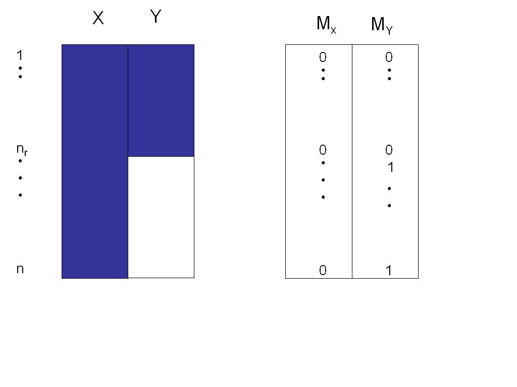
12 partial non-response data integration Missing information can be originated by data integration from dierent sources. For instance, if a unique dataset is created based on data from two dierent surveys A and B, and some variables are not surveyed in both surveys. X : variables only in A Y : variables only in B Z : variables in both A and B Interest is on the joint distribution of X, Y, Z

13 partial non-response nonresponse classifications Two main aspects of non-response are: mechanism analyzing (possibly modeling) non-response mechanism is important in order to have valid inferences. pattern sometimes pattern depends on mechanism. Applicability of dierent methods depend on nonreponse pattern.

14 partial non-response quasi randomization One possible approach to the inference on incomplete data is based on considering non-response as a second phase in sampling. However, the nonresponse mechanism is usually not under control of the researcher. Thus, validity of inferences based on respondents strongly depends on validity of assumptions made on non-response mechanism.

15 partial non-response random mechanisms involved Y N Yˆn U Population S Sample Yˆr R Respondents Design nonresponse

16 partial non-response example: simple random sampling Y = target variable for population of N units Y ˆ n sample mean (estimator of population mean) on a sample of n units: ˆ Y = n i=1 y i If there are r respondents we use the estimator Ŷ r computed on r units instead of n. is the estimator Ŷ r unbiased? is it possible to estimate its precision? it depend on the non-response mechanism. n

17 partial non-response example: simple random sampling (2) If the set of respondents can be considered as a simple random sample of the units included in the sample the estimator Ŷr is unbiased. It is a simple expansion estimator based on r units instead of n units. Of course the precision is lower since there is an increase in variance of n/r. If the hp of SRS for the (non)response is true the nonresponse mechanism is said to be completely at random (MCAR - Missing Completely at Random)

18 nonresponse mechanisms notations Y = (Y obs, Y mis ) data matrix n p Y obs Y mis observed data missing data M matrix n p of NR indicators: M ij = 0 if variable Y j is observed on the i-esima unit and 1 otherwise

19 nonresponse mechanisms nonresponse mechanisms MCAR (Missing Completely At Random) P (M Y) = P (M Y obs, Y mis ) = P (M) MAR (Missing At Random) P (M Y obs, Y mis ) = P (M Y obs ) MNAR (NMAR) (Missing Not At Random) P (M Y) cannot be simplied as in the previous cases.

20 nonresponse mechanisms intuitively.. MCAR Probability that Y mis is missing does not depend on Y (the respondents are a (simple random) sub-sample of the original sample). MAR Probability that Y mis is missing depends only on Y obs. (not on the missing values) NMAR Probability that Y mis is missing depends on Y mis ALSO upon conditioning on Y obs.

21 nonresponse mechanisms example X=class of employees classes: 1-10; 11-50; ; > 100 Y = turnover Assume that X is always observed, but Y is aected by nonresponse. If nonresponse probability P (M) is independent of Y, then the mechanism is MCAR. If, for each employee class, nonresponse probability is constant, but there are dierent probabilities in dierent classes, then the mechanism is MAR. Finally, if even within each class, nonresponse prob. depends on turnover (Y ), then we have NMAR. If we wont to estimate the mean (or total) of Y, we can get unbiased estimators only in the rt two cases (MCAR and MAR)

22 nonresponse mechanisms example(cntd) n: sample size n j : size of employees classes j (j = 1,..., 4) r: number of respondents r j : number of respondents in class j y i : turnover of ith unit(enterprise) Let: ˆ Y n = 1 n n i=1 y i Ŷ r = 1 r r y i Ŷ rj = 1 r j r j all data mean, respondent mean, respondent mean in class j, respectively i=1 i=1 y i

23 nonresponse mechanisms example(cntd) Estimators: complete data: MCAR: ˆ Y n ˆ Y r MAR: 1 n nj Ŷ rj (preferable also with MCAR) NMAR:?

24 treatment adjusting for nonresponse In the MAR case we have re-weighted units separately in dierent adjustment cells (employee classes) to reduce bias. The idea is similar to that used in sampling (randomization): If the inclusion probability for the unit i in the sample is π i, each unit represents w i = π 1 i units in the target population. w i = sampling weight. Sampling weight are known because they are determined by the sampling scheme (inverse of inclusion probabilities). Nonresponse can be viewed as a n additional selection process where, however probabilities are unknown (quasi randomization)

25 treatment adjusting for nonresponse (cntd) If nonresponse probs p ri were known for each sampled unit i, we could calculate the probability: π i = Pr ( i sampled and i respondent )= Pr( i sampled) Pr( i respondent i sampled) = π i p ri. Thus the adjusted weight would be:. π 1 i = 1 π i p ri

26 treatment adjusting for nonresponse (cntd) Usually, response probabilities are unknown. Thus, in practice one to estimate them using the available auxuliary information. In the previous example we have made the assumption that the response probability depends only on the class of employees and we have estimated this probability with rthe response rate in each class: p ri = r j /n j where j is the class of unit i. If all the sample weights are equal (w), this hypothesis leads to the estimator: ( n 4 w) 1 i j r j i w n j y i = 1 nj Ŷ rj r j n

27 treatment complete case (cc) analysis In the example, in case MAR, we used the auxiliary variable class of employees to compensate for the dierence between respondents and nonrespondents in terms of the target variable (turnover). If the mean turnover has been estimated through the mean on the whole population instead of separately for dierent classes we would have obtained a biased estimate. For Instance, if enterprises with low value of turnover have lower propensity to response, we over-estimate the turnover, because the respondents have higher values of turnover. in general, analysis based only on units where all variables are observed is said Complete Cases (CC) analysis.

28 treatment cc analysis

29 treatment advantages of cc simple (standard methods and software) no articial data (imputation) ok in case of small number of missing values and MCAR univariate estimates are comparable, in fact they are computed on the same cases.

30 treatment drawbacks of cc if nonresponse in not MCAR estimates are biased even with MCAR, some information (incomplete cases) is not used > loss of precision in the estimates

31 treatment example(1) Let (X, Y ) be Gaussian r.v.s. Assume that we have a sample of size n where X is always observed, Y has n r missing values (MCAR). We wont to estimate the expected value µ y of Y. Consider the estimator Ȳr = r i=1 y i, the mean of Y over the r respondents. If data were complete, we would use the estimator Ȳn = n i=1 y i. The ratio between the variances of the two estimators is: n/r, so for instance, if the nonresponse rate is 50%, missing values cause the rst variance become twice the second one.

32 treatment example(2) If instead of discarding the incomplete records, we use all the available information (i.e., also the X-values), we can obtain a more ecient estimator Ȳr. For instance the MLE estimator of µ y is: ˆµ yml = ˆµ y = Ȳr + ˆβ r ( X n X r ) where ˆβ r is the estimate of the regression coecient of Y on X. In this case we have: V ar(ˆµ yml )/V ar(ȳr) 1 n r n ρ2

33 treatment conclusion If ρ 2 0, then the two variances are equal, while if ρ 2 1 the variance ratio goes to r/n, i.e., we have the same gain in eciency as using the estimator Ȳn instead of Ȳr This example shows how using auxiliary information can remarkably improve the precision of the estimate if it is related to the target population parameter (in the example ρ close to 1).

34 treatment bias with cc Consider the population mean µ. We can express it in terms of the respondent mean µ r and the non-respondent mean µ nr as: thus the bias is µ = π r µ r + (1 π r )µ nr µ r µ = (1 π r )(µ r µ nr ) where π r is the respondent proportion. Thus, the estimate is unbiased only with MCAR (µ r = µ nr )

35 treatment alternatives analysis on available cases (AC) replacing missing values with articial values (imputation) analysis using all data (complete and incomplete) ( e.g. EM algorithm)

36 treatment available cases For each parameter of interest, one uses all the statistical units where the relevant variables are present. For example, we could use all the units where the variables X and Y are observed (but perhaps other variables are missing) to estimate the correlation coecient ρ xy. This method might produce inconsistent results: e.g., in each entry of the covariance matrix is estimated independently of other entries, the estimate could result in a non-positive denite matrix.

37 treatment General Strategies Complete cases??????????????? Imputation Complete-Case Analyze Analysis Incomplete Complete cases w1 w2 Complete cases Complete cases w3????? Discard????????????????????????? Imputations Weights e.g. maximum likelihood York missing data symposium 1 1

38 treatment using all data this approach includes estimation methods for incomplete data and imputation. estimation with incomplete data Under assumption of some parametric model it is sometimes possible to estimate (e.g. via ML) the parameters using also incomplete data. A popular technique is the EM algorithm. imputation the dataset is completed to obtain a rectangular dataset (without holes), replacing missing values with plausible values (imputed).

39 treatment modeling A parametric model has the advantages of being parsimonious of making the research assumptions explicit. On the other hand it is often dicult to specify a model that ts well data (e.g., zero ination, non gaussian data, etc.). In the context of ocial statistics one is usually interested in nite population quantities (e.g., totals or means), rather than in distribution parameters.

40 treatment imputation Missing values are imputed with plausible values so that standard methods and software can be applied to the completed dataset. advantages: does not require special methodology for analysis. drawbacks: an additional source of uncertainty is introduced. In the analysis phase, one should take into account the fact that imputed data are not really observed (incorporate in the estimation process the source of variability dure to nonresponse). Also, dierent may be appropriate for dierent estimations objectives.

41 non parametric (hot-deck, regression trees...) parametric (Regression, EM,...) mixed (Predictive Mean Matching,...) semi-parametric (mixture modeling,..)

42 simple methods (1) mean imputation. Missing values for each variable are imputed with the variable mean computed on the observed values. Often the population is partitioned into classes (imputation cells) and for each unit to be imputed means are computed within the class the unit belongs to. Within-cell imputation is similar to class-re-weighting within classes in sample theory. regression-based imputation. Imputed values are predictions from a regression model based on some set of covariates. Mean imputation is a particular case. One can add a random residual to the predictive mean.

43 simple methods (2) hot-deck imputation. The value to be imputed for an incomplete record is taken from a similar respondent in the same survey. This is a very common approach in the context of ocial Statistics. = exibility but dicult to make assumptions explicit. cold-deck imputation. Similar to the previous method, but imputed values are taken from a dierent survey.

44 mean imputation(1) May be appropriate if missing are MCAR (respondents are similar to non-respondents) and quantities to be estimated are means or totals (linear quantities). ȳ r : mean over r respondents out of the n sampled units. with mean imputation: 1 n ( r y i + i ) n ȳ r = 1 n (rȳ r + (n r)ȳ r ) = ȳ r r+1 since mechanism is MCAR ȳ r is an unbiased estimate of ȳ n.

45 mean imputation(2) If some non-linear parameter is to be estimated, e.g., the variance, mean imputation is not appropriate, in fact, using imputed data we would obtain: s r (n r 1)/(n 1). If s r is a consistent estimate of the population variance, the estimate resulting from mean imputation is biased (under-estimated) by (n r 1)/(n 1). in fact, mean imputation makes distribution at.

46 conditional mean imputation Using auxiliary information can improve the precision of the estimates based on imputed data. If strongly predictive covariates are available one can impute with the conditional mean. Depending on whether auxiliary variables are categorical or numerical we obtain respectively: mean imputation within strata regression imputation without residual term

47 mean imputation within cells(1) If population is divided into J cells (strata), and ȳ jr is the mean of variable Y over the r j respondents in cell j, the estimate of the mean of Y is: ȳ wc = 1 n J j=1 r j i=1 y ij + n j i=r j +1 ȳ jr = 1 n J n j ȳ jr If (on average) ȳ jr = ȳ j (MCAR) the estimator is unbiased. Note the similarity with stratication in sampling theory. j=1

48 mean imputation within cells(2) the gain deriving from imputing within cells is: V (Ȳ ) V (Ȳwc) = n 2 1 r/n r J j=1 n j n (Ȳj Ȳ )2 The dierence is large if dierences between the cell means and the overall mean is large.

49 imputation via regression without residuals (1) Missing are imputed with predictive means from (linear) regression. Simple case, 2 variables (X, Y ): y i = ˆα + ˆβx i where ˆα and ˆβ are OLS estimates based on the units where both X and Y are observed. In case where covariates are dummy variables identifying population strata, we have mean imputation within cells.

50 imputation via regression without residuals (2) Imputed values are (conditional) expected values, so although the resulting estimators of linear quantities are unbiased, the variance is under-estimated as in the case of mean imputation. In fact, the regression variance is: σ 2 Y X = σ2 Y σ2 XY σ 2 X in the imputed data Y the residual variance (non explained by the regression model) is not taken into account.

51 imputation via regression with residuals (1) In order to preserve the data variability, one can add a residual term ɛ to the imputed (conditional) mean, e.g., drawing from a normal distribution with zero mean and variance equal to the residual regression variance estimated on complete data (both X and Y ). Estimates based on this imputed dataset are nearly consistent for all population parameter as far as the imputed values can be considered random draws from the predictive distribution of missing given observed data. In the following more complex missing patterns will be analyzed.

52 hot-deck (donor) imputation (1) With hot-deck imputation values to be imputed for an incomplete record are taken from another unit (donor) where these values are available. Donor imputation includes random hot-deck and nearest neighbor donor. There are several versions: e.g., when many values are to be imputed they can all be taken from the same donor (joint imputation) or from dierent donors(sequential imputation).

53 hot-deck (donor) imputation (2) Again, assume we have to estimate the mean of Y in a population with N units. Let us assume that from in simple random sample of n units there are only r respondents. If r = n (no nonresponse)the (HT)estimator would be: ȳ n = n i=1 y i n with variance: V ar(ȳ n ) = (n 1 N 1 )S 2 y Now, we impute n r missing values via HD.

54 hot-deck (donor) imputation (3) The mean on the imputed dataset can be expressed as: ȳ HD = {rȳ r + (n r)ȳ nr}/n where ȳ r the mean on the observed values ȳ nr = r i=1 H i y i n r and H i is the number of times that y i is selected as a donor ( r i=1 H i = n r). The properties of the estimator depend on the procedure used to generate the numbers {H 1,..., H r }

55 hot-deck (donor) imputation (4) Assume random hot-deck imputation (with repetition). In this case the random vector {H 1,..., H r } can be considered as a multinomial r.v. with parameters (n r), (1/r,..., 1/r) where 1/r is the selection probability for each unit. So the expected value of each H j is (n r)/r. It follows that the expected value of ȳ HD, given the respondents is ȳ r. We know that in case MCAR respondents can be considered as a SRS of the original sample. Thus the overall expectation (i.e., with respect to the sampling and nonresponse) is: E(ȳ HD ) = Ȳ that is the estimator is unbiased.

56 hot-deck (donor) imputation (5) One can easily show that the variance is: V ar(ȳ HD ) = (r 1 N 1 )S 2 y + (1 r 1 )(1 r/n)s 2 y/n Note that the rst term is the variance of Ȳr in case of SRS of size r. We conclude that imputation causes increase of the estimate variability.

57 advantages Estimates concerning parameters of univariate distributions are approximately unbiased also for non-linear parameters, (e.g., the variance). hot-deck imputation is frequently used in practice in complex survey because it does not require model assumption (it is also applicable when data distribution is semi-continuous, e.g., zero-ination)

58 drawbacks Hot-deck imputation causes decrease of associations among observed variables and missing variables, because observed values in the record to be imputed are not taken into account. One can alleviate the problem by using covariates: hot-deck within strata nearest neighbor donor (NND) As far as the cell denition is concerned the problem is the same as in the case of mena imputation. Let us move on to NND.

59 nearest neighbor donor (nnd) Missing values in a incomplete record (recipient) are replaced with corresponding observed values in (one of) the most similar observation(s). Similarity is dened on the basis of a distance function that depends on suitably chosen covariates (matching variables). Common distance functions: l p : d p (i, j) = k x ik x jk p (p = 1 Manhattan, p = 2 euclidean) max d(i, j) = max k x ik x jk Mahalanobis d(i, j) = (x i x j ) T S 1 xx (x i x j )

60 remarks NND is asimptotic: large number of donors should be necessary (how many?) how to chose the matching variables? how to weightcontributions from dierent variables to the distance function? variables should be standardized. How? in case of many variables to be imputed, joint imputation is preferable (rather than sequential)

61 more complex methods Methods describes so far are applicable only with simple missing patterns (one variable with missing values and an always observed variable). Often data have irregular missing patterns, (holes randomly located ). More general are necessary.

62 Patterns of Missing Data General Pattern variables cases Special Patterns monotone univariate file matching York missing data symposium 1 1

63 nnd with general missing patterns Extending simple NND is simple: donor pool is composed of complete records, and the distance distance function is computed on the basis of the variables which are observed in the current recipient. For example, if we used the Euclidean distance with matching variables X 1, X 2, X 3, X 4, and in the ith unit only variables X 1 and X 3 are observed, only these two variables will be used for computing the distance with respect to potential donor j: d 2 (i, j) = (x i1 x j1 ) 2 + (x i3 x j3 ) 2

64 explicit modeling (1) We can use explicit parametric models in two ways: Regression: some variables are considered as explanatory and other as responses Joint distribution: what is modeled is the joint distribution of all variables simultaneously In any case the objective is imputing missing values with plausible values derived from the assumed model.

65 explicit modeling (2) Methods based on regression are useful when the nonresponse pattern is univariate or when variables can be splitted into always observed variables (X) and variables (Y) which are never observed on a certain subset of sampled units. In this case multiple regression of Y on X can be used. For general patterns it is better to estimate joint distribution.

66 estimation of joint distribution on cc in order to estimate parameters θ of the joint distribution of the data aected by missing values, we could use only complete records. However, this is not optimal for two reasons: 1 loss of precision (big variance) 2 risk of bias if nonresponse is not MCAR

67 estimation using incomplete data We would like to use all the available information, i.e., both complete and incomplete data. If for instance we use ML estimation, the involved probability distribution are: f(y θ) : complete data distribution f(m Y, ψ) : nonresponse (M) distribution conditional on data θ and ψ are distinct sets of parameters

68 mle We are interested in the estimates of parameters θ. ψ are nuisance parameters. Can we make inference on θ regardless of ψ-parameters (i.e., ignoring nonresponse mechanism? The answer is yes if the nonresponse mechanism is MAR: f(m Y obs, Y mis ; ψ) = f(m Y obs ; ψ) i.e., the nonresponse probability, conditional on observed data, does not depend on the non-observed data.

69 estimation under mar Using Bayes formula one can easily show that MAR hp is equivalent to assuming that the missing value distribution, conditional on observed data, is the same for respondents (M = 0) and non-respondents (M = 1): f(y mis M, Y obs ) = f(m Y obs, Y mis )f(y mis Y obs ) f(m Y obs ) = f(y mis Y obs )

70 observed data likelihood (1) In case MAR, the joint distribution of Y obs and M can be factored as product of two functions depending on θ and ψ respectively: f(y obs, M θ, ψ) = f(y obs, Y mis θ)f(m Y obs, Y mis, ψ)dy mis = = f(m Y obs, ψ) f(y obs, Y mis θ)dy mis = = f(m Y obs, ψ)f(y obs θ) L(θ Y obs ) L(θ Y obs ) observed data likelihood

71 observed data likelihood (2) Thus, MLEs can be computed by maximizing the observed likelihood L(θ Y obs ). However, this is a complex function of the target parameters maximization is not easy. An important exception is when the missing pattern is monotone, i.e. when variables Y 1,..., Y p can be ordered so that for each unit, Y k being observed implies Y j is also observed j < k. In fact, in this case the joint distribution can be factored via the chain rule as product of suitable conditional distributions whose parameters can be independently estimated.

72 n 1 n 2 f(y obs θ) = f(y i1 ; θ 1 ) f(y i2 y i1 ; β 2.1 )... n p i=1 i=1... f(y ip y i1, y i2,..., y i(p 1) ; β p.1,...,p 1 ) i=1

73 example: bivariate normal (1) V = (X, Y ) gaussian random vector. Distribution parameters: θ = (µ x, σ 2 x, µ y, σ 2 2, σ xy); X observed on n units; Y observed on n r < n units; We want to compute MLEs of the model parameters. The task is easy because the pattern is monotone.

74

75 example: bivariate normal (2) L(θ V obs ) Σ nr/2 exp { 1 2 n r i=1 σ x (n nr) exp (v i µ) t Σ 1 (v i µ) { 1 2σ 2 x re-parametrization: φ = (µ x, σ 2 x, β 0, β 1, σ 2 y x ) L(θ V obs ) σx n exp σ nr y x exp { { 1 2σ 2 y x 1 2σ 2 x i=1 n r i=1 n i=n r+1 } n (x i µ x ) 2 } (x i µ x ) 2 } (y i β 0 β 1 x i ) 2 }

76 example: bivariate normal (3) The two expressions are equivalent, but the second one can be more easily managed to obtain estimates of the parameters. In fact it is the product of the univariate lik. based on the units 1,..., n and the lik. associated to the regression of Y on X based on the units 1,... n r. Since parameters φ 1 = (µ x, σ 2 x) and φ 2 = (β 0, β 1, σ 2 y x ) are distinct, inferences can be independent. Also the rst expression is the product of two likelihood functions, but the parameters in th etwo factors are not distinct (µ x and σ 2 x are in both factors).

77 example: bivariate normal (4) MLEs can be easily derived: we use the n r units with Y observed to estimate via OLS the parameters φ 2 = (β 0, β 1, σy x 2 ) and all the units to estimate φ 1 = (µ x, σ x ) (ˆµ x = x; ˆσ x 2 = s 2 x;). Then, using re-parametrization formulas: ˆµ y = ˆβ 0 + ˆβ 1ˆµ x ; ˆσ y 2 = ˆσ y x 2 + ˆβ 1 2ˆσ2 x; ˆσ xy = ˆβ 1ˆσ x 2 Replacing the appropriate estimators in the expression for ˆµ y we obtain: ˆµ y = ȳ r + ˆβ 1 ( x x r ) where means are computed on respondents.

78 general patterns

79 em algorithm When analytic expression for MLEs are not available numerical routines have to be used. A popular method for maximization of the incomplete-data likelihood functions is the EM (Expectation-Maximization) algorithm. it allows one to obtain MLEs for incomplete data using (iteratively) standard techniques for complete data. Essentially, it is the formal version of the iterative procedure consisting of the iterative application of the following two steps: 1 replace missing values with values estimated (predicted) on the basis of the current estimates of the model parameters (E-step) 2 compute new estimates of parameters form the complete dataset imputed at the previous step (M-step)

80 em More exactly, the E-step at kth iteration is the computation of the expected value Q(θ θ (k) )of the complete data log-likelihood L(θ Y obs, Y mis ). Expectation is with respect to the distribution of missing values conditional on observed data using the current parameters θ (k) : Q(θ θ (k) ) = l(θ Y obs, Y mis )f(y mis Y obs, θ (k) )dy mis update of the estimates θ (k+1) is obtained by maximizing Q(θ θ (k) ) w.r.t. θ. Under some regularity assumptions it can be shown that the sequence θ (n) converges to the ML estimates of θ.

81 exponential family: e-step For distribution of the exponential family, log-likeluhood based on n observations y = (y 1,..., y n ) can be expressed as: l(θ Y) = η(θ) t T (Y) + ng(θ) + c where η(θ) = (η 1 (θ)), η 2 (θ)),..., η s (θ)) t, is the natural parameter, T (Y) = (T 1 (Y), T 2 (Y),..., T s (Y)) t is a s-dimensional vector of sucient statistics and c is a constant. Since l(θ Y) is linear with respect to the sucient statistics, the E-step reduces to replacing T j (Y) with E(T j (Y) Y obs, θ (t) ). For the exponential family the resulting expression is simple.

82 exponential family: m-step In the case of complete data, MLEs can be found as solution of the moment equation: E(T (Y) θ) = t where t is the realized value of T (Y) the expected value is w.r.t. f(y θ). In case of incomplete data the quantity on the r.h.s. has to be replaced by the output from the E-step. This allows explicit computation of M-step

83 example: univariate Gaussian (1) Complete data (N(µ, σ 2 )): T (Y) = (T 1 (Y), T 2 (Y)) t = ( n Y i, i=1 n i=1 Y 2 i ) t E(T 1 ) = nµ = t 1, E(T 2 ) = nσ 2 + nµ 2 = t 2 realization from (T 1, T 2 ) : where (t 1, t 2 ) are ˆµ = y ˆσ 2 = n 1 n i=1 (y i y) 2 (t 1, t 2 ) = ( n y i, i=1 n yi 2 ) i=1

84 example: univariate Gaussian (2) Incomplete data: (n 1 respondents, n 0 = n n 1 missing): E-step: n 1 n n 1 E(T 1 Y obs, θ) = E( y i + y i ) = y i + n 0 µ i=1 n 1 E(T 2 Y obs, θ) = E( yi 2 + i=n 1 +1 n i=1 n 1 i=1 i=n 1 +1 i=1 yi 2 ) = yi 2 + n 0 (σ 2 + µ 2 )

85 example: univariate Gaussian (3) M-step: [ n1 ] µ (t+1) = n 1 y i + n 0 µ (t) i=1 [ n1 ] [ n1 ] 2 σ 2(t+1) = n 1 yi 2 + n 0 σ 2(t) + n 0 µ 2(t) n 2 y i + n 0 µ (t) i=1 the above iteration converges to: ˆµ = n 1 1 ˆσ 2 = n1 1 n1 i=1 y i n1 i=1 y2 i ˆµ2. i=1

86 problems EM algorithm has to be initialized, i.e., it requires choosing (starting points) sometimes likelihood function has several local maxima. EM may converge to any of them (depending on the starting point) for some models (e.g. mixture of eteroshedastic Gaussian distributions) likelihood function is unbounded. In such cases EM may not converge.

87 imputation via em(1) For imputation purposes, EM is only an intermediate step used to estimate the distribution that generates data. In the next step, from the estimated joint distribution one has to derive the estimates of the relevant conditional distributions corresponding to various nonresponse patterns. Example: parameters: Y = (Y 1, Y 2, Y 3 ) N(µ, Σ) (µ 1, µ 2, µ 3 ; σ 11, σ 12, σ 13, σ 22, σ 23, σ 33 )

88 imputation via em(2) For the pattern where only Y 2 is missing, the parameters of the distribution: f(y 2 Y 1, Y 3 ): (α 2.13, β 2.13, σ 2.13 ) are to be estimated. These can be derived via standard formulas from the joint distribution parameters (µ, Σ) : α 2.13 = µ 2 + Σ 2(13) Σ 1 (13) µ (13) β 2.13 = Σ 2(13) Σ 1 (13) σ 2.13 = σ 22 Σ 2(13) Σ 1 (13) Σ (13)2 where Σ 2(13) is the row-vector (σ 21, σ 23 ), Σ (13) is the matrix (2 2) whose distinct elements are σ 11, σ 13, σ 33, µ (13) is the column vector (µ 1, µ 3 ) t and Σ (13)2 = Σ t 2(13)

89 alternative method More simply, one could use only complete data to estimate via standard linear all the relevant conditional distributions. However this is not optimal for two reason: 1 the parameters of the dierent conditional distributions are estimated separately rather than derived from the joint distribution parameters estimated only once 2 estimation process does not use all the available information

90 with or without residuals? Once we have estimated the distribution f(y mis Y obs ) two are possible: 1 using conditional means E(Y mis Y obs ) 2 adding a random disturbance, i.e., obtaining values to be imputed by drawing from f(y mis Y obs ). The rst method produces more accurate estimates of linear quantities such as means and totals. However, if we wont to preserve the distributional characteristics, the second method is preferable.

91 models The model most commonly used for multivariate numerical data is the Gaussian model. In fact for a lot of method and software are for incomplete normal data are available. However, often normal assumption is not realistic even after some preliminary transformation of data (e.g. logarithms, Box-Cox, etc.) In these cases some other approach may be more appropriate.

92 predictive mean matching Predictive Mean Matching (PMM) is more robust with respect to departure from normality assumption. With PMM, model is used only at an intermediate stage for computing expectations of missing given observed data. However, conditional means are not directly used for imputation. Instead, a suitable distance function is dened in terms of conditional means and used in NND imputation. The function used for NND is not a proper distance function as a function of the observed variates. The method depends to some extent on the model and does not ensures the asimptotic properties of the NND imputation. PMM can be useful when observations are not enough for NND being applied, and at the same time a full parametric approach is dicult (it is dicult to nd an explicit model tting adequately data)

93 pmm: one response variable In case of one response variable Y aected by nonresponse and p covariates (X 1,..., X p ) without missing values, PMM reduces to: for each unit u i determine the conditional expectation y i = E(Y x i1, x i2,..., x ip ) based on the estimated parameters of the regression of Y on X 1, X 2,..., X p for each u i with Y missing, impute the value y i taken from the donor u j, whose predictive mean y j is closest to y i If p = 1, PMM is the same as NND.

94 pmm: general case In the general case of arbitrary response pattern, PMM consists of the following steps: estimate the joint distribution parameters via EM algorithm for each incomplete record u i, compute the conditional mean y = E(Y mis,i y obs,i ) compute the same conditional mean for all complete records (donors) impute u i via NND using the Mahalanobis metrics based on the residual covariance matrix from the regression of Y mis on Y obs.

95 two important references Little, R. J. A. and Rubin, D. B. (2002). Statistical Analysis with Missing Data 2nd edition, Wiley. Shafer, J.L. (1997). Analysis of Incomplete Multivariate Data New York: CRC Press.