1

Transcription

1 i

2 1

3 2

4 3

5 4

6 5

7 6

8 7

9 8

10 9

11 10

12 11

13 12

14 13

15 14

16 15

17 16

18 17

19 18

20 19

21 20

22 21

23 22

24 23

25 24

26 Foreign Liabilities/ Dependen Variabel Rasio Foreign Liabilities Total Debt (1) (2) Konstanta 0.216*** 0.219*** Ekspor/Total Sales Rasio Foreign Asset 0.538*** 1.785*** R-squared N Estimator FE FE Haussman Test

27 26

28 Variabel Dependen Rasio Ekuitas Konstanta FA*Nilai Tukar *** NFA (-1) *** Nilai Tukar (-1) *** Rasio Derivatif (-1) DL (-1) *** R-Squared N Estimator Hausman Test FE Dependen Variabel Rasio Net Income Rasio EBIT Rasio Operating Rasio Interest Expenditures Coverage (1) (2) (3) (4) Konstanta *** 0.65*** *** Rasio Transaksi Derivatif Rasio EBIT Rasio Ekspor Rasio Foreign Asset *** *** 0.563*** Rasio Foreign Liabilities *** 1.125*** -1.01*** * Rasio Liabilities *** *** 2.214*** Rasio Sales *** *** Changes GM 0.511** R-squared N Estimator FE FE FE RE Haussman Test

29 28

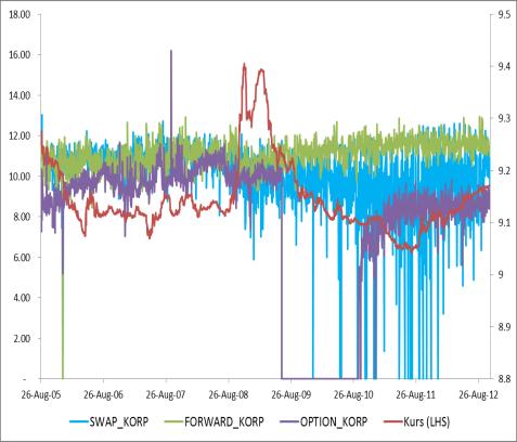
30 Variabel Level 1 st Difference CVAR * DERIVATIF_TOT * FORWARD_TOT * SWAP_TOT ** OPTION_TOT * DER_KORP * FORWARD_KORP * SWAP_KORP * OPTION_KORP * 29

31 30

32 31

33 32

34 33

35 34

36 35

37 . xtreg rfrli rexs rfras, fe Fixed-effects (within) regression Number of obs = 890 Group variable: id Number of groups = 128 R-sq: within = Obs per group: min = 5 between = avg = 7.0 overall = max = 7 F(2,760) = 8.19 corr(u_i, Xb) = Prob > F = rfrli Coef. Std. Err. t P> t [95% Conf. Interval] rexs rfras _cons sigma_u sigma_e rho (fraction of variance due to u_i) F test that all u_i=0: F(127, 760) = 6.37 Prob > F = estimates store fixed. xtreg rfrli rexs rfras, re Random-effects GLS regression Number of obs = 890 Group variable: id Number of groups = 128 R-sq: within = Obs per group: min = 5 between = avg = 7.0 overall = max = 7 Random effects u_i ~ Gaussian Wald chi2(2) = corr(u_i, X) = 0 (assumed) Prob > chi2 = rfrli Coef. Std. Err. z P> z [95% Conf. Interval] rexs rfras _cons sigma_u sigma_e rho (fraction of variance due to u_i). estimates store random. hausman fixed random Coefficients (b) (B) (b-b) sqrt(diag(v_b-v_b)) fixed random Difference S.E. rexs rfras b = consistent under Ho and Ha; obtained from xtreg B = inconsistent under Ha, efficient under Ho; obtained from xtreg Test: Ho: difference in coefficients not systematic chi2(2) = (b-b)'[(v_b-v_b)^(-1)](b-b) = Prob>chi2 =

38 . xtreg rfrtl rexs rfras, fe Fixed-effects (within) regression Number of obs = 890 Group variable: id Number of groups = 128 R-sq: within = Obs per group: min = 5 between = avg = 7.0 overall = max = 7 F(2,760) = corr(u_i, Xb) = Prob > F = rfrtl Coef. Std. Err. t P> t [95% Conf. Interval] rexs rfras _cons sigma_u sigma_e rho (fraction of variance due to u_i) F test that all u_i=0: F(127, 760) = 9.96 Prob > F = estimates store fixed. xtreg rfrtl rexs rfras, re Random-effects GLS regression Number of obs = 890 Group variable: id Number of groups = 128 R-sq: within = Obs per group: min = 5 between = avg = 7.0 overall = max = 7 Random effects u_i ~ Gaussian Wald chi2(2) = corr(u_i, X) = 0 (assumed) Prob > chi2 = rfrtl Coef. Std. Err. z P> z [95% Conf. Interval] rexs rfras _cons sigma_u sigma_e rho (fraction of variance due to u_i). estimates store random. hausman fixed random Coefficients (b) (B) (b-b) sqrt(diag(v_b-v_b)) fixed random Difference S.E. rexs rfras b = consistent under Ho and Ha; obtained from xtreg B = inconsistent under Ha, efficient under Ho; obtained from xtreg Test: Ho: difference in coefficients not systematic chi2(2) = (b-b)'[(v_b-v_b)^(-1)](b-b) = Prob>chi2 =

39 . xtreg rderb rexs rdfras rdfrli, fe Fixed-effects (within) regression Number of obs = 758 Group variable: id Number of groups = 128 R-sq: within = Obs per group: min = 4 between = avg = 5.9 overall = max = 6 F(3,627) = corr(u_i, Xb) = Prob > F = rderb Coef. Std. Err. t P> t [95% Conf. Interval] rexs rdfras rdfrli _cons sigma_u sigma_e rho (fraction of variance due to u_i) F test that all u_i=0: F(127, 627) = 0.96 Prob > F = estimates store fixed. xtreg rderb rexs rdfras rdfrli, re Random-effects GLS regression Number of obs = 758 Group variable: id Number of groups = 128 R-sq: within = Obs per group: min = 4 between = avg = 5.9 overall = max = 6 Random effects u_i ~ Gaussian Wald chi2(3) = corr(u_i, X) = 0 (assumed) Prob > chi2 = rderb Coef. Std. Err. z P> z [95% Conf. Interval] rexs rdfras rdfrli _cons sigma_u 0 sigma_e rho 0 (fraction of variance due to u_i). estimates store random. hausman fixed random Coefficients (b) (B) (b-b) sqrt(diag(v_b-v_b)) fixed random Difference S.E. rexs rdfras rdfrli b = consistent under Ho and Ha; obtained from xtreg B = inconsistent under Ha, efficient under Ho; obtained from xtreg Test: Ho: difference in coefficients not systematic chi2(3) = (b-b)'[(v_b-v_b)^(-1)](b-b) = 0.20 Prob>chi2 =

40 . xtreg rderj rexs rdfras rdfrli, fe Fixed-effects (within) regression Number of obs = 758 Group variable: id Number of groups = 128 R-sq: within = Obs per group: min = 4 between = avg = 5.9 overall = max = 6 F(3,627) = corr(u_i, Xb) = Prob > F = rderj Coef. Std. Err. t P> t [95% Conf. Interval] rexs rdfras rdfrli _cons sigma_u sigma_e rho (fraction of variance due to u_i) F test that all u_i=0: F(127, 627) = 0.96 Prob > F = estimates store fixed. xtreg rderj rexs rdfras rdfrli, re Random-effects GLS regression Number of obs = 758 Group variable: id Number of groups = 128 R-sq: within = Obs per group: min = 4 between = avg = 5.9 overall = max = 6 Random effects u_i ~ Gaussian Wald chi2(3) = corr(u_i, X) = 0 (assumed) Prob > chi2 = rderj Coef. Std. Err. z P> z [95% Conf. Interval] rexs rdfras rdfrli _cons sigma_u 0 sigma_e rho 0 (fraction of variance due to u_i). estimates store random. hausman fixed random Coefficients (b) (B) (b-b) sqrt(diag(v_b-v_b)) fixed random Difference S.E. rexs rdfras rdfrli b = consistent under Ho and Ha; obtained from xtreg B = inconsistent under Ha, efficient under Ho; obtained from xtreg Test: Ho: difference in coefficients not systematic chi2(3) = (b-b)'[(v_b-v_b)^(-1)](b-b) = 0.19 Prob>chi2 =

41 Fixed-effects (within) regression Number of obs = 756 Group variable: id Number of groups = 126 R-sq: within = Obs per group: min = 6 between = avg = 6.0 overall = max = 6 F(6,624) = corr(u_i, Xb) = Prob > F = req Coef. Std. Err. t P> t [95% Conf. Interval] rnfadkurs L rnfa L dkurs L netkumderd~s L dli L rwc _cons sigma_u sigma_e rho (fraction of variance due to u_i) F test that all u_i=0: F(125, 624) = 2.01 Prob > F =

42 . xtreg rni rdert rexs rfrli rfras rli rsa, fe Fixed-effects (within) regression Number of obs = 761 Group variable: id Number of groups = 128 R-sq: within = Obs per group: min = 4 between = avg = 5.9 overall = max = 6 F(6,627) = corr(u_i, Xb) = Prob > F = rni Coef. Std. Err. t P> t [95% Conf. Interval] rdert 3.19e rexs rfrli rfras rlia rsa _cons sigma_u sigma_e rho (fraction of variance due to u_i) F test that all u_i=0: F(127, 627) = 3.74 Prob > F = estimates store fixed. xtreg rni rdert rexs rfrli rfras rli rsa, re Random-effects GLS regression Number of obs = 761 Group variable: id Number of groups = 128 R-sq: within = Obs per group: min = 4 between = avg = 5.9 overall = max = 6 Random effects u_i ~ Gaussian Wald chi2(6) = corr(u_i, X) = 0 (assumed) Prob > chi2 = rni Coef. Std. Err. z P> z [95% Conf. Interval] rdert 4.00e rexs rfrli rfras rlia rsa _cons sigma_u sigma_e rho (fraction of variance due to u_i). estimates store random. hausman fixed random Note: the rank of the differenced variance matrix (5) does not equal the number of coefficients being tested (6); be sure this is what you expect, or there may be problems computing the test. Examine the output of your estimators for anything unexpected and possibly consider scaling your variables so that the coefficients are on a similar scale. Coefficients (b) (B) (b-b) sqrt(diag(v_b-v_b)) fixed random Difference S.E. rdert 3.19e e e-07. rexs rfrli rfras rlia rsa b = consistent under Ho and Ha; obtained from xtreg B = inconsistent under Ha, efficient under Ho; obtained from xtreg Test: Ho: difference in coefficients not systematic chi2(5) = (b-b)'[(v_b-v_b)^(-1)](b-b) = Prob>chi2 = (V_b-V_B is not positive definite) 41

43 . xtreg rebit rdert rexs rfrli rfras rli rsa, fe Fixed-effects (within) regression Number of obs = 761 Group variable: id Number of groups = 128 R-sq: within = Obs per group: min = 4 between = avg = 5.9 overall = max = 6 F(6,627) = corr(u_i, Xb) = Prob > F = rebit Coef. Std. Err. t P> t [95% Conf. Interval] rdert 5.42e rexs rfrli rfras rlia rsa _cons sigma_u sigma_e rho (fraction of variance due to u_i) F test that all u_i=0: F(127, 627) = 4.24 Prob > F = estimates store fixed. xtreg rebit rdert rexs rfrli rfras rli rsa, re Random-effects GLS regression Number of obs = 761 Group variable: id Number of groups = 128 R-sq: within = Obs per group: min = 4 between = avg = 5.9 overall = max = 6 Random effects u_i ~ Gaussian Wald chi2(6) = corr(u_i, X) = 0 (assumed) Prob > chi2 = rebit Coef. Std. Err. z P> z [95% Conf. Interval] rdert 4.88e rexs rfrli rfras rlia rsa _cons sigma_u sigma_e rho (fraction of variance due to u_i). estimates store random. hausman fixed random Note: the rank of the differenced variance matrix (5) does not equal the number of coefficients being tested (6); be sure this is what you expect, or there may be problems computing the test. Examine the output of your estimators for anything unexpected and possibly consider scaling your variables so that the coefficients are on a similar scale. Coefficients (b) (B) (b-b) sqrt(diag(v_b-v_b)) fixed random Difference S.E. rdert 5.42e e e-06. rexs rfrli rfras rlia rsa b = consistent under Ho and Ha; obtained from xtreg B = inconsistent under Ha, efficient under Ho; obtained from xtreg Test: Ho: difference in coefficients not systematic chi2(5) = (b-b)'[(v_b-v_b)^(-1)](b-b) = Prob>chi2 = (V_b-V_B is not positive definite) 42

44 . xtreg ropx rdert rexs rfrli rfras rli rsa, fe Fixed-effects (within) regression Number of obs = 761 Group variable: id Number of groups = 128 R-sq: within = Obs per group: min = 4 between = avg = 5.9 overall = max = 6 F(6,627) = corr(u_i, Xb) = Prob > F = ropx Coef. Std. Err. t P> t [95% Conf. Interval] rdert -1.16e rexs rfrli rfras rlia rsa _cons sigma_u sigma_e rho (fraction of variance due to u_i) F test that all u_i=0: F(127, 627) = 5.15 Prob > F = estimates store fixed. xtreg ropx rdert rexs rfrli rfras rli rsa, re Random-effects GLS regression Number of obs = 761 Group variable: id Number of groups = 128 R-sq: within = Obs per group: min = 4 between = avg = 5.9 overall = max = 6 Random effects u_i ~ Gaussian Wald chi2(6) = corr(u_i, X) = 0 (assumed) Prob > chi2 = ropx Coef. Std. Err. z P> z [95% Conf. Interval] rdert -2.76e rexs rfrli rfras rlia rsa _cons sigma_u sigma_e rho (fraction of variance due to u_i). estimates store random. hausman fixed random Note: the rank of the differenced variance matrix (5) does not equal the number of coefficients being tested (6); be sure this is what you expect, or there may be problems computing the test. Examine the output of your estimators for anything unexpected and possibly consider scaling your variables so that the coefficients are on a similar scale. Coefficients (b) (B) (b-b) sqrt(diag(v_b-v_b)) fixed random Difference S.E. rdert -1.16e e e-06. rexs rfrli rfras rlia rsa b = consistent under Ho and Ha; obtained from xtreg B = inconsistent under Ha, efficient under Ho; obtained from xtreg Test: Ho: difference in coefficients not systematic chi2(5) = (b-b)'[(v_b-v_b)^(-1)](b-b) = Prob>chi2 = (V_b-V_B is not positive definite) 43

45 44

46 45

47 46

48 47

49 48

50 49

51 50

52 51

53 52

54 53

55 54

56 55

57 56

58 57

59 58

60 59

61 60

62 61