Lecture 4: Generalized Linear Mixed Models

Transcription

1 Dankmar Böhning Southampton Statistical Sciences Research Institute University of Southampton, UK S 3 RI, December 2014

2 An example with one random effect An example with two nested random effects

3 An example with one random effect An example: health awareness study three states in the US participated in a health awareness study each state independently devised a health awareness program three cities within each state were selected for participation and five households within each city were randomly selected to evaluate the effectiveness of the program a composite index (a count number) was formed (the large the index, the greater the awareness) the data have the following hierarchical structure:

4 An example with one random effect data: household state city

5 An example with one random effect Poisson model with random effect for state for the health awareness index Y ijk for household k, in city j, and state i: log E[Y ijk ] αi = log µ ijk = µ + α i with a state random effect α i N(0, σ 2 S ) and a Poisson error Y ijk Po(µ ijk )

6 An example with one random effect Poisson model with random effect for state let P(Y ijk = y) = Po(y µ ijk ) = Po(y µ + α i ) likelihood L = Po(y ijk µ + α i ) i,j,k (in the fixed effect case) but α i N(0, σs 2 ), e.g. normal random, so L = Po(y ijk µ + α i )φ(α i )dα i i α i j,k where φ(α i ) is a normal density with mean 0 and variance σ 2 S

7 An example with one random effect

8 An example with one random effect Mixed-effects Poisson regression Number of obs = 45 Group variable: state Number of groups = 3 Obs per group: min = 15 avg = 15.0 max = 15 Integration points = 1 Wald chi2(0) =. Log likelihood = Prob > chi2 =. index IRR Std. Err. z P> z [95% Conf. Interval] _cons Random-effects Parameters Estimate Std. Err. [95% Conf. Interval] state: Identity sd(_cons) LR test vs. Poisson regression: chibar2(01) = Prob>=chibar2 = Note: log-likelihood calculations are based on the Laplacian approximation.

9 An example with two nested random effects Poisson model with random effect for state and random effect for city nested within state let P(Y ijk = y) = Po(y µ ijk ) = Po(y µ + α i + β j(i) ) where β j(i) N(0, σt 2 ), e.g. normal random likelihood L = i α i β j j Po(y ijk µ + α i + β j(i) )φ(β j )dβ j φ(α i )dα i k where φ(α i ) is a normal density with mean 0 and variance σ 2 S where φ(β j ) is a normal density with mean 0 and variance σ 2 T

10 An example with two nested random effects

11 An example with two nested random effects Mixed-effects Poisson regression Number of obs = 45 No. of Observations per Group Integration Group Variable Groups Minimum Average Maximum Points state city Wald chi2(0) =. Log likelihood = Prob > chi2 =. index IRR Std. Err. z P> z [95% Conf. Interval] _cons Random-effects Parameters Estimate Std. Err. [95% Conf. Interval] state: Identity sd(_cons) city: Identity sd(_cons) 7.65e LR test vs. Poisson regression: chi2(2) = Prob > chi2 = Note: LR test is conservative and provided only for reference. Note: log-likelihood calculations are based on the Laplacian approximation.

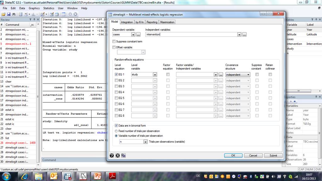
12 Meta-Analysis on BCG vaccine against tuberculosis Colditz et al. 1974, JAMA provide a meta-analysis to examine the efficacy of BCG vaccine against tuberculosis

13 Data on the meta-analysis of BCG and TB the data contain the following details 13 studies each study contains: TB cases for BCG intervention number at risk for BCG intervention TB cases for control number at risk for control also two covariates are given: year of study and latitude expressed in degrees from equator

14 intervention control study year latitude TB cases total TB cases total

15 Data analysis on the meta-analysis of BCG and TB these kind of data can be analyzed by taking TB case as disease occurrence response intervention as exposure (fixed effect) study as random effect latitude and year as further fixed effects

16 Mixed Logistic Regression Model log p xij 1 p xij = µ + α i + β INTER INTER ij + β LAT LAT ij where α i N(0, σ 2 S ) each trial arm within each study contributes a binomial likelihood ( nij y ij ) p y ij x ij (1 p xij ) n ij y ij where p xij = exp(µ + α i + β INTER INTER ij + β LAT LAT ij ) 1 + exp(µ + α i + β INTER INTER ij + β LAT LAT ij )

17 Mixed Logistic Likelihood L = i ( nij α i y ij j ) p y ij x ij (1 p xij ) n ij y ij φ(α i )dα i where φ(α i ) is a normal density with mean 0 and variance σ 2 S

18

19 Integration points = 1 Wald chi2(1) = Log likelihood = Prob > chi2 = cases Odds Ratio Std. Err. z P> z [95% Conf. Interval] intervention _cons Random-effects Parameters Estimate Std. Err. [95% Conf. Interval] study: Identity sd(_cons) LR test vs. logistic regression: chibar2(01) = Prob>=chibar2 = Note: log-likelihood calculations are based on the Laplacian approximation..

20 Integration points = 1 Wald chi2(2) = Log likelihood = Prob > chi2 = cases Odds Ratio Std. Err. z P> z [95% Conf. Interval] intervention latitude _cons Random-effects Parameters Estimate Std. Err. [95% Conf. Interval] study: Identity sd(_cons) LR test vs. logistic regression: chibar2(01) = Prob>=chibar2 =

21 Integration points = 1 Wald chi2(3) = Log likelihood = Prob > chi2 = cases Odds Ratio Std. Err. z P> z [95% Conf. Interval] intervention latitude year _cons Random-effects Parameters Estimate Std. Err. [95% Conf. Interval] study: Identity sd(_cons) LR test vs. logistic regression: chibar2(01) = Prob>=chibar2 =

22 Integration points = 1 Wald chi2(2) = Log likelihood = Prob > chi2 = cases Odds Ratio Std. Err. z P> z [95% Conf. Interval] intervention year _cons Random-effects Parameters Estimate Std. Err. [95% Conf. Interval] study: Identity sd(_cons) LR test vs. logistic regression: chibar2(01) = Prob>=chibar2 =

23 model evaluation model log L AIC BIC intervention latitude year latitude