Testing the Limits of Latent Class Analysis. Ingrid Carlson Wurpts

Transcription

1 Testing the Limits of Latent Class Analysis by Ingrid Carlson Wurpts A Thesis Presented in Partial Fulfillment of the Requirements for the Degree Master of Arts Approved April 2012 by the Graduate Supervisory Committee: Leona Aiken, Co-Chair Christian Geiser, Co-Chair Stephen West ARIZONA STATE UNIVERSITY May 2012

2 ABSTRACT The purpose of this study was to examine under which conditions "good" data characteristics can compensate for "poor" characteristics in Latent Class Analysis (LCA), as well as to set forth guidelines regarding the minimum sample size and ideal number and quality of indicators. In particular, we studied to which extent including a larger number of high quality indicators can compensate for a small sample size in LCA. The results suggest that in general, larger sample size, more indicators, higher quality of indicators, and a larger covariate effect correspond to more converged and proper replications, as well as fewer boundary estimates and less parameter bias. Based on the results, it is not recommended to use LCA with sample sizes lower than N = 100, and to use many high quality indicators and at least one strong covariate when using sample sizes less than N = 500. i

3 TABLE OF CONTENTS Page LIST OF TABLES... iv LIST OF FIGURES... v CHAPTER 1 INTRODUCTION... 1 Model Parameters in LCA... 2 Previous Research on the Performance of LCA... 3 Research Questions METHOD Simulation Conditions and Procedure Label Switching Problem Dependent Variables RESULTS Non-converged Solutions Improper Solutions Boundary Parameter Estimates Standard Error Outliers Parameter Bias Standard Error Bias Estimated Covariate Power ii

4 CHAPTER Page 4 DISCUSSION Sample Size Number of Indicators Indicator Quality Use of a Covariate ML Versus MLR Estimation Planning and LCA Study Limitations and Suggestions for Future Research REFERENCES iii

5 LIST OF TABLES Table Page 1. Summary of Population Specifications for Class Proportions, Class Profiles, and Indicator Quality Acceptable Exclusion Criteria, Parameter Bias, and SE Bias for Selected 2-Class ML Conditions Acceptable Exclusion Criteria, Parameter Bias, and SE Bias for Selected 2-Class MLR Conditions Acceptable Exclusion Criteria, Parameter Bias, and SE Bias for Selected 3-Class ML Conditions Acceptable Exclusion Criteria, Parameter Bias, and SE Bias for Selected 3-Class MLR Conditions iv

6 LIST OF FIGURES Figure Page 1. Label switching in 2-Class conditions Label switching in 3-Class conditions Non-convergence in 2-Class conditions Non -convergence in 3-Class conditions Improper solutions in 2-Class conditions Improper solutions in 3-Class conditions Boundary parameter estimates in 2-Class conditions Boundary parameter estimates in 3-Class conditions Covariate SE in 3-Class ML low quality conditions Covariate SE in 3-Class ML low quality conditions, outliers excluded SE outliers in 2-Class conditions SE outliers in 3-Class conditions Total analyzed replications in 2-Class conditions Total analyzed replications in 3-Class conditions Class 1 bias in 2-Class conditions Class 2 bias in 2-Class conditions Class 1 bias in 3-Class conditions Class 2 bias in 3-Class conditions Class 3 bias in 3-Class conditions High CRP bias in 2-Class conditions v

7 Figure Page 21. Low CRP bias in 2-Class conditions High CRP bias in 3-Class conditions Low CRP bias in 3-Class conditions Covariate bias in 2-Class conditions Covariate bias in 3-Class conditions Class 1 SE bias in 2-Class conditions Class 1 SE bias in 3-Class conditions Class 2 SE bias in 3-Class conditions Class 3 SE bias in 3-Class conditions High CRP SE bias in 2-Class conditions Low CRP SE bias in 2-Class conditions High CRP SE bias in 3-Class conditions Low CRP SE bias in 3-Class conditions Covariate SE bias in 2-Class conditions Covariate SE bias in 3-Class conditions Estimated covariate power in 2-Class conditions Estimated covariate power in 3-Class conditions Conditions with acceptable bias in 2-Class conditions Conditions with acceptable bias in 3-Class conditions vi

8 Chapter 1 INTRODUCTION Latent Class Analysis is a type of latent variable mixture model; it operates under the assumption that there are various latent (unobserved) subgroups within the population, and these subgroups respond differently to a set of observed items or indicators (Vermunt & Magidson, 2004). LCA is used in many disciplines within in the social sciences. For example, Geiser, Lehmann, and Eid (2006) used LCA to identify five subgroups of individuals who differed quantitatively and qualitatively in what strategy they used to solve a set of mental rotations tasks. LCA has also been used in clinical populations to identify discrete subgroups of young adults who self-injure (Klonsky & Olino, 2008). LCA classification of eating disorder patients has been shown to have better predictive validity of mortality rates than classifications based on the DSM-IV (Crow, Swanson, Peterson, Crosby, Wonderlich, & Mitchell, 2011). Furthermore, LCA models can be extended to accommodate multiple groups, covariates, and longitudinal data (Collins & Lanza, 2010). Even though Latent Class Analysis (LCA) is becoming increasingly popular among social science researchers, it is still a relatively new modeling technique. There have not been many studies which explore the limiting conditions of LCA application. In particular, there are no straightforward guidelines about the minimum sample size necessary for LCA, or the impact of having many or few indicators of the latent class variable. Currently available guidelines about minimum sample size or optimal number of indicators in LCA 1

9 are either discrepant, or have not been based on thorough simulation studies. Also, researchers are interested in the importance of the quality of the indicators used. Obviously using the best quality indicators would be ideal. However, this many not always be possible in practice. Therefore, the question arises, under what conditions can lower quality indicators be used and still produce reliable and unbiased results? In the same vein, to which extent can high quality indicators compensate for a small sample size? Is adding more indicators beneficial or detrimental to the quality of estimation in LCA? This simulation study explores the impact of these and other conditions on model estimation and parameter bias in LCA. Model Parameters in LCA The prevalence or relative size a subgroup is called the class proportion, and all class proportions must sum to one. The probability of a subject responding in a specific way to a certain item, given the individual s class membership is called the conditional response probability (CRP), and these parameters can take on any value between 0 and 1. For example, a CRP of.83 for dichotomous indicator 3 in Class 1 means that for each individual in Class 1, his or her probability of answering correctly or affirmatively to indicator 3 is.83. There are two types of model parameters in classical LCA: class proportion parameters, and item parameters. Let L be the latent class variable with c = 1,, C categories (or classes). Then γ c = P(L = c) is the unconditional probability of membership in latent class c; it also indicates the proportion of individuals in the particular class, or the relative size of the class. Let ρ j,rj c = P(u j = r j L = c) be 2

10 the conditional probability of choosing category r j for item j given membership in class c. This, the CRP, gives the probability of an individual endorsing a specific item category, given the individual is in a certain class. CRPs are particular to each item and class. LCA models can also include covariates which predict class membership via logistic regression. Given a covariate X, the probability of membership in class c can be expressed as P(L = c X = x) = for c = 1,, C -1 (Collins & Lanza, 2010). In this logistic regression equation, e β1c represents the odds ratio (OR), or the change in odds of latent class membership between class c and the reference class C for every one-unit change in X. Note that in logistic regression, an arbitrary reference class must be chosen. Certain software programs (e.g., Mplus; Muthén & Muthén, ) automatically choose the last class as reference in LCA. The inclusion of a covariate in the model does not change the interpretation of CRPs, but it does change the interpretation of the class proportion parameters, which are now conditional on different values of X. Previous Research on the Performance of LCA In general, adding indicators to an LCA model increases the number of model-implied response patterns such that many of these patterns may have low response frequency. This problem, called data sparseness, occurs when the 3

11 contingency table of all possible item response patterns contains many empty cells. This often leads to biased p-values of the chi-square model goodness-of-fit (Langeheine, Pannekoek, & Van De Pol, 1996) and an increase in the number of boundary parameter estimates (Galindo-Garre & Vermunt, 2006). Data sparseness often occurs when the sample size is small, but can also occur if there are many indicators or when too many classes are estimated (Uebersax, 2000). Because of this, researchers may be tempted to use a smaller number of indicators when running LCA models. On the other hand, Marsh, Hau, Balla, and Grayson (1998), who varied the number and quality of indicators in a simulation study of confirmatory factor analysis (CFA) models, found that using more highquality indicators per factor results in several advantages: more converged solutions, more proper solutions, and less parameter bias. These advantages were even more pronounced for smaller sample sizes. Similarly, in a study of Latent Transition Analysis (LTA), a longitudinal extension of LCA, Collins and Wugalter (1992) suggested that adding additional indicators to latent class models can outweigh the disadvantage of data sparseness by reducing standard errors. Although Collins and Wugalter s findings point in the same direction as Marsh et al. s results, there has been no systematic research regarding whether this principle of more is better, especially in small sample sizes, generalizes to classical LCA. Although there has been no rigorous simulation work to advise general sample size guidelines for LCA, there have been studies of the performance of various model fit statistics under different sample size conditions in the more 4

12 general Latent Variable Mixture Modeling (LVMM). Nylund, Asparouhov, and Muthén (2007) used simulated sample sizes of N = 200, N = 500, and N = 1000 to test the performance of likelihood-based tests and Information Criteria in determining the number of latent classes in mixture modeling. They found that while the bootstrap likelihood ratio test and the adjusted Bayesian Information Criterion could fairly accurately identify the correct number of latent classes in sample sizes of N = 500 and N = 1000, these statistics were much less accurate at N = 200. Henson, Riese, and Kim (2007) also showed that with N = 500, relative model fit statistics were generally not powerful enough to differentiate between the correct number of components in LVMM; furthermore, they showed that parameter bias was highest when N = 500, and decreased in the N = 1,500 and N = 2,500 conditions. Lo, Mendell, and Rubin (2001) found that the adjusted Lo- Mendell-Rubin statistic had low power to detect the correct number of classes when N = 300 or less. Collins and Wugalter (1992) found that a sufficiently large sample size helps ensure good parameter recovery in LTA when there are few indicators, and they suggest a minimum N of somewhat smaller than 300, although they only tested N = 300 and N = 1,000 conditions. Tueller and Lubke (2011) examined structural equation mixture models (SEMM; a combination of structural equation and mixture models) and suggest a minimum sample size ranging from N = 300 to N = 1000 based on how well the classes are separated, although SEMM is not directly comparable to classical LCA. Overall, Finch and 5

13 Bronk (2011) suggest that N = 500 is a worthy goal for researchers using classical LCA. Also, indicator quality or how close the CRPs are to 1 or 0 is also a factor of interest. High quality indicators are generally desirable for interpretation. However, Galindo-Garre and Vermunt (2006) inspected the logit parameterizations of LCA indicators with extreme population values. They found that indicators with extreme population values had the largest logit estimates, tending towards infinity; these represent boundary estimates in the logit parameterization of the LCA model. Also, these estimates were in general much larger for sample sizes of N = 100 rather than N = 1000 (Galindo-Garre & Vermunt, 2006). In general, CRPs are found to be much closer to the boundary for sample sizes of N = 100 rather than N = 1000 (Galindo-Garre & Vermunt, 2006). Still, there is evidence of benefits to having high quality indicators, at least in the context of structural equation models with continuous latent variables (Marsh et al., 1998). Also, having sufficiently high quality indicators i.e., indicators with CRPs of.9/.1, could compensate for having too few indicators and aid parameter recovery in LTA models. (Collins & Wugalter, 1992). There is also a dearth of empirical simulation studies examining the use of covariates in LCA. Covariates can be related to LCA models by several different methods, but the single-step inclusion method, used here, has shown to best recover the true covariate parameter effect, and to have the highest power and coverage of the effect (Clark & Muthén, 2009). However, Clark and Muthén s simulation only considered 2-Class models with 10 indicators, and two covariate 6

14 logistic regression loading sizes (0.5 and 0); further simulation studies are needed to determine whether these findings hold for more diverse models. Also, this particular simulation only examined competing methods of covariate inclusion and only reported outcomes related to the covariate effect. None of the conditions were compared to similar conditions without a covariate, and none of the other model parameters (class proportion bias, CRP bias) were reported. However, it has been recommended that incorporating covariates into a growth mixture model can aid in enumerating the number of classes (Muthén, 2004). Other simulation work has examined the use of covariates in factor mixture models (a combination of LCA and common factor analysis) and found that increasing the covariate effect size leads to a higher proportion of individuals assigned to the correct class, even if class separation was poor (Lubke & Muthén, 2007). However, these models were not compared to a model without covariates, and other outcomes, such as the recovery of parameters of the measurement model, were not studied. In using real data to estimate an SEMM with and without covariates, the model with covariates performed better, as determined by the BIC (Vermunt & Magidson, 2005). Further simulation work is needed to determine whether the addtion of covariates is beneficial for classical LCA models. Mplus offers two types of standard error estimators: maximum likelihood (ML) and maximum likelihood robust (MLR). The MLR estimator was designed to be more robust to likelihood misspecification (B. O. Muthén, ). In a limited Monte Carlo simulation with small sample sizes and correct likelihood 7

15 specification, the MLR estimator has shown to provide better standard errors than the ML estimator, although both are used by applied researchers doing LCA (B. O. Muthén, ). However, more research is needed to determine whether these sample size recommendations generalize to classical LCA (which uses categorical latent variables and categorical indicators) and whether for other factors for example, the number and quality of indicators, the presence of a covariate, and the type of estimator can compensate for low sample size. In summary, very few studies have examined the performance of LCA models, and those that exist have only looked at LCA under a limited set of conditions. As LCA becomes more popular, it is important for researchers to recognize under which conditions LCA yields reliable and unbiased results, as well as which conditions should be particularly avoided. The goal of this study was to examine in detail different conditions that are particularly relevant for practical applications, and provide guidelines for applied researchers regarding the limiting conditions of LCA: minimum sample size, ideal number and quality of indicators, use of covariates, type of standard error estimator used, and under what conditions can certain good data characteristics compensate for poor characteristics? Research Questions This present study was designed to provide answers to the following questions: What is the minimum sample size that is feasible under the conditions examined here? Is using more indicators beneficial to parameter recovery? How 8

16 much does the quality of indicators affect parameter recovery? How does the inclusion and effect size of a covariate affect parameter recovery? Is ML or MLR estimation better? What characteristics of a study can compensate for poor data characteristics? It was expected that conditions of at least N = 500 will perform consistently well, following Finch and Bronk (2011), and that conditions below this size, especially below N = 300 may be problematic (Henson, Riese, & Kim, 2007). Although the Marsh et al. simulation examined CFA models and there is no guarantee that these results will generalize to LCA, it was also expected that adding more high quality indicators would outweigh the problems of data sparseness (Marsh et al., 1998, Collins & Wugalter, 1992). High quality indicators were expected to be related to better CRP and CRP SE bias (Collins & Wugalter, 1992), but also more frequent occurrence of boundary parameter estimates, at least in small sample sizes (Galindo-Garre and Vermunt, 2006). However, in the Marsh et al. (1998) simulation, indicator quality was confounded with number of indicators, so it remains to be seen if adding more low quality indicators, or increasing indicator quality without increasing the number of indicators, affects results. It was expected that conditions with a large covariate effect size would show good parameter recovery and low standard error bias (Clark & Muthén, 2009), and that models with a covariate would perform better in general than models without a covariate (Vermunt & Magidson, 2005). MLR estimation was expected to perform better than ML estimation in the small sample size conditions (Muthén, ). The answers to these questions should 9

17 serve to give applied researchers thorough recommendations regarding the use of LCA under a wide variety of conditions. 10

18 Simulation Conditions and Procedure Chapter 2 METHOD characteristics: The simulation followed a factorial design with six manipulated data Number of classes: 2, 3 Number of indicators: 4, 5, 6, 7, 8, 9, 10, 11, 12 Effect of covariate on latent class membership: none, small, moderate, large Quality of indicators: low vs. moderate vs. high Type of standard error: ML vs. MLR Sample size: 70, 100, 200, 300, 500, 1000, 2000 All data characteristics are were fully crossed, except in two cases: first, for the 3-Class models, the 4-indicator condition is intrinsically underidentified, and so none of these models were studied (Collins & Lanza, 2010). Second, the set of 2-class models was estimated first with only low and high quality indicators, but after examination of preliminary results, a third moderate quality condition was added to the 3-class models. There were 7 (sample size) x 9 (number of indicators) x 2 (quality of indicators) x 4 (covariate effect) x 2 (standard error estimation) = 1,008 2-class conditions, plus 7 x 8 x 3 x 4 x 2 = 11

19 1,344 3-class conditions totaling 2,352 conditions for the entire simulation. There were 1000 replications for each condition. The independent variables and their respective levels were chosen based on the methods and results of previous SEM and LCA Monte Carlo studies, common findings in substantive research, as well as my own results from a pilot study. Following Marsh et al. (1998), the number of indicators was varied between 4 and 12 to examine whether their more is better suggestion generalizes to LCA, and in particular, whether more high-quality indicators can compensate for low sample size. The number of classes chosen was 2 and 3 because 2- and 3-class models are often estimated in substantive research, and these models also allow exploration of the minimal indicator conditions 4 and 5 indicators, respectively. In the 2-class models, Class 1 was generated to have a class proportion parameter of γ c =.67, so Class 2 was generated with γ c =.33, because Σγ c = 1 by definition of the LCA model. In the 3-class models, the γ c parameters were.4,.4, and.2 for classes 1, 2, and 3, respectively. These class proportions were chosen to reflect common class proportions found in substantive research rarely are all of the classes exactly equal in size; often there is at least one class that is about twice the size of another class. Class profiles were also assigned following Collins and Wugalter (1992) and Nylund et al. (2007) so that Class 1 had high CRPs for all items, Class 2 had high CRPs for half of the items, and low for the other half, and in the 3-class models, Class 3 had low CRPs for all items. See Table 1 for the specific class profiles. 12

20 Mplus requires model specification in terms of logit intercept (or threshold ) parameters. With R j response categories, Mplus requires R j -1 logit thresholds, with the last response category as the reference category. For C classes, Mplus requires C 1 logit thresholds, with the last class as the reference class. This means that Mplus also outputs parameter estimates as logit thresholds. Although these thresholds carry the same information as CRPs and class proportions, they are not as intuitive to interpret. This can easily be overcome by using the MODEL CONSTRAINT command to specify new parameters that simply convert the logit thresholds into class proportions and CRPs and estimate their standard errors as well. Because these class proportions and CRPs contain no new information beyond the logit parameters, the model fit remains the same. All indicators had two response categories, and were generated as locally independent, conditional on latent class membership. High and low quality CRP parameters were chosen following Collins and Wugalter s (1992) strong and weak measurement strength conditions. The indicators in the high quality conditions were generated to either have CRPs (of endorsing the second category) of.9 or.1, while the low quality indicators were generated at.7 or.3. The moderate quality condition with CRPs of.8 and.2 was added after seeing large differences in parameter bias between low and high quality conditions. Exploring these intermediate conditions is useful not only because of the large decrease in parameter bias when moving from low to high quality indicators, but also because extremely high quality indicators are less commonly seen in practice CRPs of 13

21 .7/.3 or.8/.2 are much more common. See Table 1 for a summary of class profiles and class proportion and indicator quality conditions. The continuous covariate X was generated from a normal distribution with a variance of 1 and a mean of 0. The size of the covariate effect was chosen following Rosenthal s (1996) effect size conventions for the odds ratio (OR = e β1c ), where odds ratios of 1.5, 2.5, and 4.0 describe small, moderate, and large covariate effect sizes, respectively. The covariate effect must be specified with logistic regression slope coefficients, β 1c = log(or), and logistic regression intercept coefficients β 0c. In the 2-class models, there is only (2-1) = 1 β 1c parameter to estimate, but in the 3-class models, there are (3-1) = 2 β 1c parameters; in this latter case, both were generated to be the same, within each covariate effect size condition. Also, when a non-zero covariate effect is included in the model, the γ c parameters change for different values of X. The covariate intercept parameter β 0c reflects class proportions when X = 0, which in this case is the mean of the covariate. To be consistent with the no-covariate conditions, in the covariate conditions, the covariate intercepts β 0c were specified to be the same as the latent class thresholds in the corresponding no-covariate conditions, such that the class sizes at the mean of X in the covariate conditions were the same as the unconditional class sizes in the no-covariate conditions. Even though N = 500 has been recommended as a worthy goal by Finch and Bronk (2011), a sample of this magnitude may often be unrealistic for applied researchers. Thus, smaller and more attainable sample size conditions of N = 300, 14

22 N = 200, and N = 100 were used for a pilot simulation and included in the final simulation as well. However, in the pilot simulation, N = 100 was found to have acceptably low class proportion bias in some conditions when using high quality indicators. So, a condition of N = 70 was also included to explore the lower limit of sample size in LCA application. Henson, et al. (2007) showed that sample size and accuracy of likelihood-based statistics improves vastly from N = 500 to N = 1,500, but only moderately from N = 1,500 to N = 2,500. So, N = 2*500 = 1,000 and N = 2*1,000 = 2,000 conditions were included to explore larger sample sizes in LCA, and whether there is a point at which larger N does not continue to meaningfully improve parameter bias and estimation. Mplus 6 was both used to generate the data, using the MONTE CARLO command, and also to fit a correctly specified LCA model to the data. The true population parameters were used as starting values for the estimation in each replication to decrease computing time and to avoid label switching (see discussion below) and the occurrence of local maxima as much as possible (Collins & Lanza, 2010). I wrote a SAS macro to automatically create the 2,352 Mplus data generation files and 2,352,000 Mplus estimation files, as well as a batch file that automatically executes all of the Mplus files. Label Switching Problem In LCA solutions, there are c! possible labeling permutations of c classes, so that even with data generated by well-separated and homogeneous classes, there is the possibility that the parameter estimates may not match the labels of the generated data, which leads to the problem of label switching. This is an 15

23 important issue to consider in simulation studies. Obviously, it would not make sense, for example, to aggregate Class 1 parameter estimates across replications if some of the solutions have switched labels and the class 1 parameter estimates actually refer to Class 2. Although label switching can often be detected by inspecting the solution, this method is unreliable and subjective when the estimated parameters vary greatly from the generating parameters (e.g., due to high sampling error in small samples). Also, any sort of manual inspection of each individual solution is simply not feasible in such a large simulation. Tueller, Drotar, and Lubke (2011) developed an algorithm implemented in the software R that uses true class assignment and estimated class assignment data saved from Mplus to check if label switching has occurred in an LCA solution. The program outputs whether each replication has correct class labels, incorrect labels, or incorrigible labels, meaning the program could not reliably determine if label switching had occurred, usually due to the class assignment matrix not meeting the program s minimum criteria for class assignment accuracy. All incorrigible or incorrectly labeled models were counted and excluded from the final analysis. 1 The population parameter values were used as starting values for each replication of the simulation in order to increase estimation speed and minimize label switching; however, it was still important to determine if any solutions displayed label switching, to ensure class-specific parameter estimates could be properly aggregated within a condition. A trivial amount of models were detected as label switched and subsequently excluded from further analysis. A larger 16

24 problem was the proportion of models which did not meet the criterion for the label switching algorithm to correctly work ( incorrigible replications). The program used to detect label switching only works if the class assignment accuracy, as defined by the conditional proportion correct assignment (the proportion of subjects correctly assigned within each class,) is moderately greater than chance. In order for the label switching detection algorithm to work correctly, the conditional proportion correct assignment must be greater than 1/c in c 1 classes. In models where there are very few low quality indicators, the class assignment accuracy will likely be low and so the model is not amenable to detection of any label switching. These models were marked as incorrigible and also excluded from further analysis. Although there were very few incorrigible models in the high and moderate quality indicator conditions, many of the low quality conditions had at least one third of their replications marked as incorrigible. Improved indicator quality had the largest impact on reducing the number of incorrigible models; increasing the size of the covariate effect and the number of indicators also decreased incidence of incorrigibility, while increasing sample size had a somewhat smaller positive impact. In the 2-Class high quality conditions, the maximum amount of replications excluded per condition for being incorrigible was 1.3%, and a total of only one high quality model was excluded as incorrigible among all the 3-class conditions. The moderate quality conditions also had fairly low instances of incorrigible models: 12.5% of models were excluded in the N = 70, 5-indicator 17

25 conditions, but this number quickly dropped as sample size, number of indicators, and strength of the covariate increased (see Figure 1). Low quality models, however, were much more problematic. In the 2- Class low quality conditions, the maximum proportion of incorrigible models was near 75% at N = 70. Even at N = 2000, without a large covariate effect, the 4- and 5-indicator models had 40-74% of their replications excluded due to incorrigible label switching. Low quality models performed slightly better in the 3-Class conditions: the maximum proportion incorrigible per condition with N = 70 was 51.7%, while in the N = 2000 conditions, the maximum proportion incorrigible was 30% (see Figure 2). There were a very few replications that were actually label switched, and these replications were excluded as well. In total, 217,289 replications were excluded from the analysis for being incorrigible or label switched. Dependent Variables The dependent variables examined include: 1. Number of models excluded from analysis for non-convergence. 2. Number of models excluded from analysis for suspected label switching. 3. Number of models excluded from the analysis because of improper solutions. 4. Number of boundary parameter estimates. 18

26 5. Number of replications with abnormally large standard errors. 6. Relative parameter estimate bias for class proportions, CRPs, and odds ratio of the covariate effect. 7. Relative standard error bias for class proportions, CRPs, and odds ratio of the covariate effect. 8. Estimated power of the covariate regression slope coefficient. The number and type of model estimation problems, as indicated by Mplus warning messages and excluding boundary parameter errors was recorded. Common problematic errors included: The model estimation did not terminate normally due to an ill-conditioned Fisher Information Matrix. Change your model and/or starting values. The standard errors of the model parameter estimates may not be trustworthy for some parameters due to a non-positive definite first-order derivative product matrix. The model estimation has reached a saddle point or a point where the observed and the expected information matrices do not match. Any replications with clear signs of estimation problems, except for solutions that showed boundary parameter estimates as the only problem and otherwise seemed to be properly identified, were also excluded from the final analysis, which was conducted in both SAS 9.3 and SPSS (All graphs were created in SPSS or R.) 19

27 Another outcome of interest was the number of boundary parameters in each condition. Boundary parameter estimates are CRPs (or class proportions) that have been estimated at the boundary of the probability space: exactly 1 or 0. They have no standard error, which makes computing a significance test or confidence interval for the parameter impossible (Galindo-Garre & Vermunt, 2006). Here the focus will be on the much more common CRP boundary estimates. Boundary estimates generally occur when there is data sparseness or the contingency table of all possible item response patterns contains many empty cells (Galindo-Garre & Vermunt, 2006). This is often the case when the sample size is small, but can also occur if there are many indicators or many classes are estimated (Uebersax, 2000). Although some people believe the occurrence of boundary estimates is inconsequential, their presence can cause numerical problems in estimation algorithms, (Vermunt & Magidson, 2004) as well as problems in computing the parameter s asymptotic variance-covariate matrix, (Galindo-Garre & Vermunt, 2006) and they can be a sign of convergence to local maximum solutions or underidentified models (Uebersax, 2000). This later problem is often undesirable because if the parameter estimates are based on a local maximum of the likelihood function, then they may vary drastically in multiple runs of the estimation. Also, a solution with many boundary parameters may be difficult to interpret (Uebersax, 2000). Thus boundary parameters present both statistical and substantive difficulties. 20

28 Even though solutions containing boundary parameters are not necessarily problematic, their prevalence is of interest, because boundary parameter estimates may indicate specific problems in estimation. Individual boundary parameters were counted, but the parameters (and their respective standard errors, which are always zero) were not included in the aggregated average CRP parameter bias calculations. Even when excluding replications with Mplus warning messages about untrustworthy standard errors, there still remained many proper replications with extremely large standard errors, estimated as high as 20 in some replications. These large outlying standard errors would give a large positive skew to the SE distributions within each condition. Even with no Mplus warning messages, applied researchers would probably not interpret a solution with such large standard errors. Replications with excessively large SEs can also be excluded from proper replications in simulation studies (Marsh et al., 1998). Therefore, any replication with an outlying standard error was not included in the calculation of parameter bias. Outliers were defined as those values exceeding 1.5*interquartile range (IQR) more than the 75th percentile or 1.5*IQR less than the 25th percentile. This also helped to make the distribution of the SEs much more symmetric, so that the mean of the distribution could be used in the calculation of bias. Relative bias was calculated by subtracting the true value of the parameter from the mean of the simulated parameter estimates across all replications and dividing the difference by the parameter s true value. Relative standard error bias 21

29 was calculated similarly by finding the difference between the mean of the standard errors of the parameter estimates across replications and the standard deviation of parameter estimates across replications and dividing this difference by the standard deviation of parameter estimates. The mean parameter estimate bias and standard error bias were calculated for all proper replications. In the case of CRPs, bias was averaged only among indicators generated with the same CRP, i.e., in the low-quality condition, the biases of all CRPs generated at.7 are averaged, and the biases of all CRPs generated at.3 are averaged. (See Table 1 for class profiles.) In 2-Class conditions, only two high CRPs and two low CRPs were averaged in each replication, instead of averaging all non-boundary CRPs in each replication. This was done because even within each quality condition, the high and low CRPs had different population values and so the bias could potentially differ because of these values. Also, the 4-indicator conditions had only two low CRPs, and so comparing the average of two of every type of indicator in each replication allowed a fair comparison of parameter bias across conditions with different numbers of indicators. In 3-Class conditions, four CRPs each of high and low indicators were averaged. Class proportion estimate bias was calculated separately for each class. In the covariate conditions, the covariate intercept parameters β 0c (converted into probability scale) were used to examine bias in the class proportion estimates as they reflect conditional class proportions at X = 0, that is, at the mean of the covariate X. In this case, because β 0c was specified to be equal to the logit class 22

30 proportions of the non-covariate conditions, bias is still calculated and interpreted in the same way. Estimated power to detect the covariate effect is the probability of rejecting H 0 : β 1c = 0 given that β 1c is not equal to zero in the population; in the present study, power was estimated as the percent of significant (at α =.05) β 1c parameters among all proper replications in each condition (Muthén & Muthén, 2002). Power was only calculated for those replications where the parameter was not overbiased more than10% and the covariate standard error was not underbiased more than 10%.In the 2-class model there was only one β 1c parameter (converted into an odds ratio OR = e β1c ) for the covariate effect. In the 3-class model, the relative parameter estimate bias and standard error bias of the two β 1c parameters (converted into odds ratios) were averaged, as they were both generated to be the same value. Similarly, the estimated covariate power was averaged for both β 1c parameters in the 3-class models. All of these outcomes, taken together, will be able to give a good picture of what data characteristics researchers should avoid, such as low sample size combined with poor quality indicators, as well as general guidelines for minimum sample size, optimal number of indicators, and in what cases good data characteristics can compensate for poor ones. 23

31 Chapter 3 RESULTS Non-converged Solutions Overall, non-convergence was mostly related to small sample size, fewer indicators, and low quality indicators. Moderate quality indicator conditions (those with CRPs of.8 or.2) overall had a maximum of 2.8% non-convergence, and high quality indicator conditions (those with CRPs of.9 or.1) had less than 1% non-convergence. As seen in Figure 3, the maximum percent of low quality non-converged 2-Class models per condition was 22.6%, and the maximum percent of low quality non-converged 3-Class models per condition was 16.7%, as seen in Figure 4 for the smallest sample size condition of N = 70. By N = 200, the incidence of non-convergence was 10% for both 2- and 3-Class models. Also, in high quality 2-Class models with low sample size, there were several replications (2-6 per condition) for which the generated data on one variable were all equal due to sampling error, meaning that the variance for this variable was zero and the model could not be estimated. In total, 14,307 (0.6%) of all replications did not converge. Improper Solutions All models with any estimation error message (except for boundary parameter messages) in the output were marked as improper and excluded from the final analysis. The number and type of output errors in each condition was also examined as a dependent variable. 24

32 The pattern of improper solutions differed between the N = and N 200 conditions (see Figure 5 and Figure 6). When the sample size was very small (N = ) and the indicators were high quality, increasing the number of indicators increased the number of improper solutions, particularly the number of error messages about untrustworthy standard errors. By comparison, with low or moderate quality indicators and a very small sample size, the lowest number of improper solutions was found with a medium number of indicators. In all conditions with N 200, the number of improper solutions was reduced by increasing the number of indicators, the size of the covariate effect, the quality of the indicators, and the sample size, with a few exceptions. The 4- and 5- indicator conditions actually showed an increasing proportion of improper solutions as the sample size got larger, especially for the high quality models. In the high quality 2-Class models with no covariate, the 4- and 5- indicator models often had untrustworthy standard errors, suggesting that some of these models may be empirically underidentified. It is difficult to determine whether mixture models such as LCA are identified (Muthén, ). In total, of all converged replications had improper solutions, which is 3.5% of the overall replications and 3.51% relative to all converged replications. Boundary Parameter Estimates The frequency of boundary parameter estimates was assessed by calculating the proportion of boundary parameter estimates per total number of independent CRP parameters in each model. This proportion was averaged across all proper models in each condition. The maximum mean proportion of boundary 25

33 parameter estimates was almost 27% in the 3-Class N = 70, high quality, 5- indicator, no covariate condition. In general, increasing sample size, number of indicators, and size of the covariate effect all decreased the incidence of boundary parameters. The relationship between indicator quality and the number of boundary parameters was more complex. With few indicators (4 or 5) or very small sample sizes (N = 70), the high quality models had more boundary parameter estimates than the low quality models, as seen in Figure 7. However, excluding the 4- and 5- indicator models and the N = 70 conditions, the prevalence of boundary solutions for the low quality models was equal to or higher than for the high quality models. The moderate quality indicators in general showed the lowest number of boundary parameter estimates (see Figure 8). Standard Error Outliers Figure 9 shows the distributions of the covariate standard error estimates in the 3-Class, ML, low quality conditions. The estimated standard errors are very large often near 10, and in one case above 60. The distributions of the covariate SE estimates in the same conditions are shown in Figure 10. While the distributions are still somewhat skewed in the smaller sample sizes, the remaining values are not outrageous and would be considered acceptable by most researchers. The covariate SE parameters overall showed the largest outliers and the most skew, but the other SE parameters showed similar patterns. In general, more indicators corresponded to more replications excluded for any SE outlier, except that the 2-Class 4- and 5-indicator conditions often had the 26

34 highest number of replications with SE outliers (see Figure 11). Also, MLR conditions had a higher prevalence of SE outliers (see Figure 12). In total, 659,754 replications (28% of the total replications, and 32.4% of all correctly labeled, converged, and proper replications), were excluded for containing at least one outlying standard error. Note that after removing different numbers of replications from each condition, due to outlying SEs, the parameter bias was calculated based on different replications in corresponding ML and MLR conditions. Thus the relative parameter bias sometimes differed between ML and MLR conditions, but this was an artifact of the differential exclusion of replications based on their standard errors, rather than a true difference in parameter recovery between ML and MLR; more MLR replications were excluded for having large SEs, as the distributions of SEs in the MLR conditions were particularly skewed in the low indicator quality conditions. These two estimation methods only affect the estimation of the standard errors, not the parameters. The parameter bias results are only reported here for ML estimation conditions. Figures 13 and 14 display the number of replications in each condition that met the criteria to be analyzed for parameter bias, i.e. the replications that converged, had correct class labels, had proper solutions, and contained no standard error outliers. In 2-Class conditions, high quality conditions generally had at least 800 usable replications. However, in 2-Class low quality conditions, the number of usable replications varied from less than 200 with 4 indicators to over 500 with 12 indicators and a small sample size, or over 800 with 12 27

35 indicators and large sample size. In 3-Class conditions, high quality conditions usually had at least 600 usable replications, but as few as 400 for N = 70 and indicators, or large sample sizes with 5 indicators. Moderate quality 3-Class conditions had similar patterns to high quality conditions, except that most of the moderate quality conditions with N = had usable replications. In 3-Class low quality conditions, the number of usable replications varied from around 200 with 4 indicators to over 400 with 12 indicators and a small sample size, or over 600 with 12 indicators and large sample size. The following parameter bias results should be interpreted together with the information from Figures 13 and 14. That is, the low parameter bias in a certain condition might be based on very few usable replications, and thus does not imply that the condition is good overall, but rather that in the small amount of proper replications, the parameters were unbiased. The parameter and SE bias results are based on 1,378,579 replications, or 58.6% of the original replications. The results presented here also focus on what is the ideal number of indicators for each sample size, as researchers are often more limited in the size of the sample they are able to collect than in the number of measures. Even if it is not mentioned specifically, in most conditions examined here, as sample size increases, fewer indicators may be used, and vice versa. Parameter Bias Class proportion bias. The two most important factors in reducing class proportion bias were increasing the number of indicators, as well as increasing the indicator quality. The presence and increasing magnitude of the covariate effect 28

36 corresponded to lower class proportion bias as well. Larger sample sizes also somewhat helped decrease bias, especially in the 3-Class conditions. Class proportion bias in 2-Class conditions. Class proportion bias for Class 1 (the larger class) was less than 10% in all high indicator quality conditions, as well as all low indicator quality, large covariate effect size conditions (see Figure 15). Class 1 bias was less than 10% for low indicator quality, moderate covariate effect size conditions with 7-12 indicators. Class 1 bias was also less than 10% for low indicator quality, small or no covariate conditions with 8-12 indicators. Class proportion bias for Class 2 (the smaller class) was less than 10% in all high indicator quality conditions, except the no covariate, N = 2000, 4- and 5- indicator conditions (see Figure 16). Low indicator quality, large covariate effect size conditions had bias less than 10% with N 100 and 6-12 indicators. Low indicator quality conditions with a moderate covariate effect had bias less than 10% with N 100 and 9-12 indicators. Low indicator quality, small covariate effect conditions had bias less than 10% with N 200 and indicators or N 1000 and 8-12 indicators. Low quality conditions with no covariate had bias less than 10% with N = 200 and indicators, or N 300 and indicators, or N 1000 and 8-12 indicators. All low indicator quality conditions with N = 70 and 12 indicators also had acceptable bias. Class proportion bias in 3-Class conditions. The Class 1 proportion bias was less than 10% in all 3-Class conditions (see Figure 17). The class proportion bias for Class 2 and Class 3 was less than 10% in all high and moderate quality 29

37 indicator conditions. Most, but not all, low indicator quality conditions with 6-12 indicators had Class 2 proportion bias less than 10% (see Figure 18). Low quality conditions with a large covariate effect size had Class 3 proportion bias generally less than 10% with 6-12 indicators (see Figure 19). Low quality conditions with a moderate covariate effect size had Class 3 proportion bias less than 10% with 8-12 indicators. Low quality conditions with N 100 and no covariate or a small covariate effect size had Class 3 proportion bias less than 10% with 9-12 indicators. In low quality conditions, 9-10 indicators generally had the lowest bias. CRP Bias. Larger sample size, higher indicator quality, and a greater number of indicators generally helped reduce CRP bias. Increasing indicator quality and sample size were the two most influential factors in decreasing CRP bias for high CRP indicators and larger sample sizes also reduced low CRP indicator bias. However, for the low CRP indicators, the highest overall bias was in the high quality 4- and 5- indicator conditions. Adding more indicators decreased bias for low CRPs, especially with low quality or low sample size conditions. The effect of the covariate effect size was not apparent for the high CRPs, but a larger covariate effect size did seem to decrease bias for the low CRPs, especially in low quality conditions. In 3-Class conditions with low sample sizes, the moderate quality conditions had the lowest bias for low CRP indicators, and the high quality conditions had the highest bias for low CRP indicators. 30

38 CRP bias in 2-Class conditions. All CRP bias in the 2-Class conditions was less than 1.5% for the high CRP indicators, that is, those with population values of.7 or.9 (see Figure 20). Note that high CRPs are different from high quality CRPs. However, there were many conditions in which the low CRP indicators were biased more than 10% (see Figure 21). High indicator quality conditions had low CRP bias less than 10% with N 100 and 6-12 indicators. With N = 70 and high quality indicators, only the moderate and large covariate effect size conditions with 10 indicators had acceptable low CRP bias. With low quality indicators and a large covariate effect, all conditions had low CRP bias less than 10%. Using a moderate covariate and low quality indicators, low CRP bias was less than 10% at N 70 and 7-12 indicators. Using a small covariate and low quality indicators, low CRP bias was less than 10% at N 70 and indicators. With low quality indicators and no covariate, low CRP bias was less than 10% with N 70 and indicators, or N 200 and 8-12 indicators. CRP bias in 3-Class conditions. High CRP indicators had bias less than 4% in all 3-Class conditions (see Figure 22). Low CRP indicators had bias less than 10% in high quality conditions with a large covariate effect size, N 100, and 6-12 indicators; with a moderate covariate effect size, N 100, and 9-12 indicators; or with no or a small covariate effect size, N 200, and 6-12 indicators (see Figure 23). 31

39 Low CRP indicators had bias less than 10% in moderate quality conditions with a large covariate effect size, N 70, and 8-12 indicators; with a moderate covariate effect size, N 70, and indicators; with a small covariate effect size, N 70, and indicators; or with no covariate, N 100, and 7-12 indicators. All moderate quality conditions with N 200 had acceptable low CRP bias using 6-12 indicators. Low quality conditions with N 200 had low CRP bias less than 10%, except N = 200, no covariate, 5-indicator condition. Other low quality conditions with low CRP bias less than 10% were N = 70, with a large covariate effect, and indicators; N = 100, with a large covariate effect, and 4-12 indicators; N = 70, with a moderate covariate effect and 12 indicators; and N = 100, with a moderate covariate effect and 7-12 indicators; Covariate Bias. Larger sample sizes, more indicators, and higher indicator quality all corresponded to lower covariate bias. The effects of sample size and number and quality of indicators were much more pronounced in low quality or low sample size conditions. The effect size of the covariate had little relationship to covariate bias, although in some smaller sample size conditions, bias decreased with smaller covariate effect sizes. Covariate bias in 2-Class conditions. At N = 70, high quality conditions with 6-12 indicators had bias less than 10% (see Figure 24). All high quality conditions with N 100 had bias less than 10% except in one condition (N = 100, 4 indicators, small covariate effect size.) With a large covariate effect size, low quality conditions had bias less than 10% with N 200 and 8-12 indicators. With 32

40 a moderate covariate effect size, low quality conditions had bias less than 10% with N = 70 and N 300 with 5-12 indicators; there were several N = conditions with acceptable bias, but the pattern was much less clear. Low quality conditions with a small covariate effect size mostly had bias less than 10% with N 70 and 6-12 indicators. Covariate bias in 3-Class conditions. All high quality conditions had bias less than 10%, except the N = 70, 6-indicator, large covariate condition (see Figure 25). Moderate quality conditions with N = 70, a large or moderate covariate effect, size and 8-12 indicators had bias less than 10%. Moderate quality conditions with N 70, a small covariate effect, size and 5-12 indicators had bias less than 10%. Almost all moderate quality conditions had bias less than 10% with N 100. Low quality, large covariate effect size conditions with N 100 and 8-12 indicators had bias less than 10%, although conditions with 8-9 indicators generally had the lowest bias. Low quality, moderate covariate effect size conditions with at N 200 and 8-12 indicators had acceptable bias. All low quality, small covariate effect conditions with N 100 had bias less than 10%. There were several low quality, N = 70 conditions with bias less than 10%, but there was no factor within these conditions that consistently contributed to decreased bias. Standard Error Bias Class Proportion SE Bias. Increasing sample sizes, adding more indicators, and increasing indicator quality all generally corresponded to lower 33

41 class proportion SE bias. Overall, the most consistent factor seemed to be quality: higher quality conditions had less bias. Increasing the covariate effect size also decreased bias in 2-Class, large sample size, low indicator quality conditions. Sample size seemed to have little effect on the bias in high quality conditions, but larger sample sizes corresponded to lower bias especially in 3-Class moderate and low indicator quality conditions. However, in 2-Class low indicator quality conditions, bias somewhat increased with larger sample sizes. Bias generally decreased with more indicators; however, the bias remained unchanged or increased with more indicators when N was small and the indicator quality was low. The MLR estimator performed slightly better for moderate to low sample sizes (N 500), and the ML estimator performed slightly better for large sample sizes (N 1000), although this difference was most appreciable in the low indicator quality conditions. Class proportion SE bias in 2-Class conditions. All high quality conditions with 6-12 indicators had bias less than 10%, and high quality conditions with N 300, 4-5 indicators, and a large or moderate covariate effect had bias less than 10% (see Figure 26). Low quality conditions had noticeably fewer conditions with acceptable bias. Bias was less than 10% in low quality conditions when using a large covariate, 6-12 indicators, and N 500. In low quality, moderate covariate effect size conditions, bias was generally less than 10% with 8-12 indicators and N 500. In low quality, small covariate conditions, bias was generally less than 10% 34

42 with indicators and N 500. With no covariate, low quality conditions consistently showed bias less than 10% only with 12 indicators and N 300. Below N = 500, the low indicator quality conditions with bias less than 10% were very sparse, except that at N = 100, using MLR estimation and any size covariate, conditions with 4-9 indicators ha bias less than 10%. Class proportion SE bias in 3-Class conditions. In high quality conditions, Class 1 SE bias was generally less than 10% for N 70, 6-12 indicators, and a moderate or large covariate; N 100, 6-12 indicators, and a small covariate; or N 200, 6-12 indicators, and no covariate (see Figure 27). In moderate quality conditions, Class 1 SE bias was generally less than 10% for N = 200, 8-12 indicators, and ML estimation; or, for N = 200, 6-12 indicators, and MLR estimation. In moderate quality conditions with N 300, 6-12 indicators, and ML or MLR estimation, Class 1 SE bias was generally less than 10%, although there were still several conditions that had bias slightly more than 10%. In low quality conditions with ML estimation, Class 1 SE bias was less than 10% with N 1000 and 8-12 indicators. In low quality MLR conditions, there was no consistent pattern of conditions with Class 1 SE bias less than 10%, but almost no conditions with N < 300 had acceptable bias. In high quality conditions with any size covariate, conditions with 6-12 indicators generally had Class 2 SE bias less than 10% (see Figure 28). In high quality conditions with no covariate and N 100, conditions with 6-10 indicators generally had Class 2 SE bias less than 10%. In moderate quality conditions with N = 200 and ML estimation, conditions with 8-12 indicators generally had Class 2 35

43 SE bias less than 10%. In moderate quality conditions with N = 200 and MLR estimation, conditions with 7-12 indicators generally had Class 2 SE bias less than 10%. In moderate quality, N 300, ML conditions with 6-12 indicators generally had acceptable Class 2 SE bias. In moderate quality, N 300, MLR conditions with 8-12 indicators generally had acceptable Class 2 SE bias. Using low quality indicators and ML estimation, only conditions with N = 500 and indicators or N 1000 and 8-12 indicators consistently had Class 2 SE bias less than 10%. Using low quality indicators and MLR estimation, there was no consistent pattern of conditions with Class 2 SE bias less than 10%, but almost no conditions with N < 300 had acceptable bias. High quality indicator conditions with no covariate generally had Class 3 SE bias less than 10% with N 100 and 5-11 indicators (see Figure 29). High quality indicator conditions with a small covariate effect size generally had Class 3 SE bias less than 10% with N 70 and 5-11 indicators. High quality indicator conditions with a moderate or large covariate effect size generally had Class 3 SE bias less than 10% with N 70 and 5-12 indicators. Moderate quality indicator conditions with N = always had Class 3 SE bias less than 10% with 12 indicators. Moderate quality conditions with N = 200 generally had Class 3 SE bias less than 10% with 8-12 indicators. Moderate quality conditions with N 300 generally had Class 3 SE bias less than 10% with 5-12 indicators. Low quality indicator conditions with N = 500 and ML estimation had Class 3 SE bias less than 10% with 8-12 indicators and a large covariate, 9-12 indicators and a moderate covariate effect size, indicators and a small 36

44 covariate effect size, or 12 indicators and no covariate. With N 1000 and ML estimation, most conditions with 5-12 indicators had Class 3 SE bias less than 10%. Low quality indicator conditions with N = 300 and MLR estimation had Class 3 SE bias less than 10% with indicators and a large or moderate covariate, indicators and a small covariate effect size, or 11 indicators and no covariate. With N 500 and MLR estimation, most conditions with 5-12 indicators had Class 3 SE bias less than 10%. CRP SE Bias. CRP SE bias decreased with larger sample sizes, along with more and better quality indicators. Increasing sample size had a small effect on the high CRPs in the lower quality conditions, but had a negative effect on the low CRPs in some of the lower quality conditions. Increasing indicator quality overall had a positive effect on decreasing bias, but with low sample sizes, moderate quality indicators had the lowest bias. The number of indicators had little effect on the high CRPs, but with low-quality low CRPs, the more indicators corresponded to less bias. MLR conditions had somewhat less bias, especially in low and moderate quality conditions with fewer indicators. Covariate effect size only decreased bias in the 2-Class, large sample size, low quality conditions. CRP SE bias in 2-Class conditions. All high quality conditions had high CRP SE bias less than 10%, except with 4 indicators, no covariate, and N 500 (see Figure 30). In general, low quality conditions had the lowest bias with 11 indicators. Low quality conditions with N 200 and a large or moderate covariate had CRP SE bias less than 10%, except with N = 200, 6 indicators, and a moderate covariate effect size. With low quality indicators, N 300, and a 37

45 small covariate effect size, all conditions had CRP SE bias less than 10% except N = 500, 4 indicators. With low quality indicators, N 300, 5-12 indicators, and no covariate, all conditions had CRP SE bias less than 10% except the N = 1000, 5-indicator condition. For the high quality conditions, low CRP SEs had bias less than 10% with N 200, at least 5 indicators and no covariate (except N = 300 and 5 indicators) or at least 6 indicators and small or moderate covariate effect, or at least 4 indicators, and a large covariate effect (see Figure 31). Low CRP SEs in the low quality conditions had a more complicated pattern of bias. With no covariate and N 200, all conditions with at least 10 indicators had bias less than 10%. With a small covariate, N 200 and at least 8 indicators, all conditions except one (N = 1000, 9 indicators) had low CRP SE bias less than 10%. With a moderate covariate, N 200 and at least 8 indicators, low CRP SE bias was less than 10%. With a large covariate, N 200 and at least 7 indicators, low CRP SE bias was less than 10%. CRP SE bias in 3-Class conditions. High quality conditions had high CRP SE bias less than 10% with 6-12 indicators and N 100, as well as most conditions at N = 70 (see Figure32). Note that from N = , there were several high quality 5 indicator conditions with high CRP SE bias less than 10%. All moderate quality conditions had high CRP SE bias less than 10% with 6-12 indicators and N 200, as well as 8-12 indicators and N = Low quality ML conditions with N = 500 and indicators, or N 1000 with 8-12 indicators had high CRP SE bias less than 10%. High CRP SE 38

46 bias was less than 10% in only five low quality ML conditions with N 300. Low quality MLR conditions with N = 200 and 9-12 indicators, or N 300 and 6-12 indicators had high CRP SE bias less than 10%. Low quality MLR conditions with N = and moderate or large covariate effect sizes had high CRP SE bias less than 10% with indicators. Large sample sizes were generally related to smaller low CRP SE bias in the 3-Class conditions, especially with high or low quality indicators (see Figure 33). However, in the low quality, MLR conditions, larger sample size was actually related to higher SE bias. Indicator quality was another important factor, but the lowest bias occurred with the moderate quality indicators, while the low quality indicators had the most bias. The covariate effect did not seem to be very influential. The type of standard error estimator did not seem to make much difference for high or moderate quality conditions, but MLR seemed to have lower bias with low quality, small sample size conditions, and ML had lower bias with low quality, large sample size conditions. All high quality conditions with N 200 and a small, moderate, or no covariate had low CRP SE bias less than 10%, except in the N = 200, 5-indicator, MLR, no covariate condition. All high quality conditions with N 100 and a large covariate had low CRP SE bias less than 10%, except in the N = 100, 5- indicator, MLR condition. All moderate quality conditions with any covariate effect size had low CRP SE bias less than 10% with two exceptions: N = 200, small covariate, 5- indicator, MLR condition, or N = 70, moderate covariate, 8-indicator condition, 39

47 ML condition. All moderate quality conditions with no covariate and ML estimation had low CRP SE bias less than 10%, except the N = 100, 8-indicator condition. All moderate quality conditions with no covariate, MLR estimation, and at least 7 indicators had low CRP SE bias less than 10%. Low quality conditions with ML estimation only had low CRP SE bias consistently less than 10% with N 1000, or with N 500 and a large covariate effect. Low quality MLR conditions had low CRP SE bias less than 10% for almost all conditions N = 70- N = 300. With N 500, low quality, and MLR estimation, low CRP SE bias was only consistently less than 10% with at least 8 indicators, except in the N = 1000, small covariate, 11-indicator condition. Covariate SE Bias. In general, larger sample size, higher number and quality of indicators, and greater effect size of the covariate all led to reduced covariate standard error bias. Increasing sample size had a positive effect on reducing covariate SE bias especially in the low quality conditions. Higher quality conditions also showed less bias than lower quality conditions, particularly with small sample sizes. Covariate SE bias for 2-Class conditions. All high quality conditions at N 200 had bias less than 10% (see Figure 34). All low quality conditions with 6-12 indicators and N 1000 had bias less than 10%. In general, increasing the number of indicators also reduced covariate SE bias, except that in most low quality cases, the 5-indicator conditions were more biased than the 4-indicator conditions. Larger covariate effect size also decreased bias in the low sample size, low quality conditions. However, as the sample size increased, the effect of 40

48 the covariate effect size became much less pronounced, and with higher sample sizes, the small covariate effect conditions were the least biased. For N = 200 through N = 500, the low quality MLR conditions were less biased than the low quality ML conditions. There were no notable differences between ML and MLR in the remaining conditions. Covariate SE bias in 3-Class conditions. All high quality conditions had covariate SE bias less than 10% (see Figure 35). Moderate quality conditions with N 100 had bias less than 10% with a large covariate effect size, or a moderate covariate effect size and 7-12 indicators. Moderate quality conditions with N 200 and a moderate covariate effect size had bias less than 10%, as well as moderate quality conditions with a small covariate effect size, at least 8 indicators, and N 500, or N 1000 for any number of indicators. Estimated Covariate Power Increasing sample size, increasing the number and quality of indicators, as well as increasing the covariate effect size all increased estimated covariate power. Increasing the number of indicators especially increased power in the 3- Class conditions. Increasing the covariate effect size increased power especially between the small and moderate covariate effect size conditions. Even though ML conditions generally had higher covariate SE bias, power was only computed for replications with acceptable bias, and ML estimation conditions generally showed higher power than MLR estimation conditions. Estimated Covariate Power in 2-Class Conditions. With a small covariate effect, high quality indicators, and N = 300, conditions with

49 indicators had power above 80% (see Figure 36). With a small covariate effect, high quality indicators, and N 500, conditions with 4-12 indicators had power above 80%. With a moderate covariate effect, high quality indicators, ML estimation, and N = 70, conditions with 6-12 indicators had power above 80%. With a moderate covariate effect, high quality indicators, MLR estimation, and N = 100, conditions with 6-12 indicators had power above 80%. With a moderate covariate effect and high quality indicators, conditions with ML estimation and N 100 or conditions with MLR estimation and N 200 had power above 80% with 4-12 indicators. High quality, large covariate effect size conditions had power above 80%, except the 4- and 5-indicator MLR conditions with N = 70. Estimated Covariate Power in 3-Class Conditions. Conditions with N = 70 had power greater than 80% with either high quality indicators and a large covariate effect, or with moderate quality indicators, a large covariate effect, at least 8 indicators, and ML estimation (see Figure 37). Conditions with N = 100 and high quality indicators had power greater than 80% with either a large covariate effect, or a moderate covariate effect, 7-12 indicators, and ML estimation, or with a moderate covariate effect, indicators, and MLR estimation. Most conditions with N 200 had power greater 80% with high or moderate quality indicators and a large or moderate covariate effect size, or with low quality indicators, a large covariate effect size, and ML estimation. Most conditions with N 500 had power greater than 80% with high quality indicators or with low quality indicators and a large or moderate covariate effect size. 42

50 Nearly all conditions with N 1000 had power greater than 80%, except a few of the 5-8 low quality indicator, small covariate effect size conditions. 43

51 Chapter 4 DISCUSSION With LCA becoming increasingly popular across diverse fields within the social sciences, it is important to determine under which conditions LCA performs well, and under which conditions it performs poorly. To date, there have been very few simulation studies examining LCA performance regarding the minimum sample size, ideal number and quality of indicators, and use of covariates. Although current research suggests a minimum sample size of N = 500 (Finch & Bronk, 2011), as well as the benefits of having more indicators (Marsh et al., 1998, Collins & Wugalter, 1992), higher quality indicators (Collins & Wugalter, 1992), adding a covariate, and using the MLR estimator (Muthén, ), these findings have either been taken from the SEM or LVMM literature in general, or they have not been based on comprehensive simulation work. The present study sought to provide recommendations for LCA applications regarding these data characteristics by simulating 1000 data sets for each of 2352 conditions, and estimating a correct model for every condition. Replications with potential label switching were removed, as were any with an improper solution or an abnormally large standard error. The parameter and standard error relative bias was examined in the remaining conditions. The results generally support the expected outcomes: conditions with at least N = 500 performed well, although there were many conditions as low as N = 100 that displayed acceptable parameter and SE bias. Also, the addition of more 44

52 indicators had a positive effect on reducing the bias of almost every type of parameter and SE, as did increasing indicator quality, as well as adding and increasing the effect size of a covariate. MLR estimation conditions also generally had lower SE bias than ML estimation conditions. This study is the first to study LCA under so many conditions, and the results clearly indicate which factors are important in increasing convergence and proper solutions, as well as decreasing parameter and SE bias. Sample Size Many applied researchers are limited in the size of the sample data they can gather, and there exist no empirically tested guidelines regarding the minimum sample size for using LCA. Based on the existing literature (e.g., Finch & Bronk, 2011), it was expected that conditions with at least N = 500 would perform well, with conditions below N = 300 performing poorly. According to the results of the present simulation study, when estimating 2 classes, sample sizes as small as N = 100 result in reliable results as long as at least 6 indicators of high quality (i.e., if CRPs are very high or very low) are used. With low quality indicators, the minimum sample size recommended is N = 500, and only with at least l1-12 indicators, or 8-12 indicators and a moderate or large covariate (see Figure 38, Table 2, and Table 3). When estimating 3 classes, sample sizes as small as N = 100 can be used with 6-12 high quality indicators and a large covariate, or 9-12 high quality indicators and a moderate covariate. With N 200, at least 6 high quality indicators should be used with or without a covariate. With 3 classes and only 45

53 moderate quality indicators, sample sizes lower than N = 200 should be avoided, unless there are 12 indicators. With N = 200, at 9-12 moderate quality indicators should be used, or 6-12 moderate quality indicators and N = 300. With low quality indicators, sample sizes below N = 500 are not generally recommended, and N = 500 should not be used unless using 12 indicators, or at least 10 indicators and a moderate or strong covariate. Above N = 1000, at least 6 low quality indictors will suffice (see Figure 39, Table 4, and Table 5). Note that for some factors expected to have very good outcomes, i.e. N = 2000, there were conditions that still did not have all parameter and SE bias less than 10%. This was often because one of the class proportion SE bias averages was slightly larger than the strict cut-off of 10% usually no more than 15% bias. These findings extend previous suggestions about the minimum recommended sample size for LCA. In addition, they are very important in highlighting what factors can compensate for a lower sample size higher number and quality of indicators, adding a covariate and which factors require higher sample sizes lower number and quality of indicators. These results will give researchers using LCA a better idea of the minimum sample size they should strive for, as well as the type and number of indicators and covariates they should attempt to use. Number of Indicators One of the key factors examined here was the influence of the number of indicators, and whether adding more indicators is beneficial, following the results of Marsh et al. (1998). The answer is that yes, having more indicators is generally 46

54 beneficial with a few exceptions. At the smallest sample size condition of N = 70, especially in the 3-Class conditions, adding more indicators resulted in more improper solutions up to half of the replications in some cases. This could be because with such a small sample size and so many estimated parameters, the data contingency table was too sparse (Uebersax, 2000). Also, adding more indicators often contributed to more replications being excluded for abnormally large standard errors. However, this is logical as adding more indicators means that there are more SEs to be estimated and thus more of a chance that one of them will be large. Still, adding more indicators usually reduced or did not affect parameter and SE bias, as expected (Marsh, et al., 1998, Collins & Wugalter, 1992), except in the case of class proportion SE bias in small N, 2-Class conditions and low SE bias in small N, 2- and 3-Class conditions. Note that the 4- and 5- indicator models were very problematic, with the highest number of improper replications, boundary parameter estimates, and often the highest parameter or SE bias. This could be because the particular population class profiles chosen for these models often resulted in empirically underidentified solutions. The replication may have passed the Mplus criterion for identification while it was in fact underidentified. More simulations should be done to see whether the 4- and 5- indicator conditions are generally problematic, or whether they perform better with different class profiles. Further studies should examine whether these trends apply to models with many more indicators, such as 20 or more: there may be a point at which, even with a reasonably large sample size, having too many indicators is bad. 47

55 Indicator Quality Another key factor of interest to this study was the quality of indicators: whether higher quality indicators are always better, and if indicator quality can compensate for low sample size. The answer here is for the most part yes increasing indicator quality almost always improves outcomes, even beyond just parameter recovery (Collins & Wugalter, 1992). Higher quality indicator conditions were associated with fewer incorrigible or label switched solutions, fewer non-converged replications, fewer improper replications (except with N = 70), fewer replications with SE outliers, lower parameter bias (except for low CRP bias and low CRP SE bias in the N = or 4- and 5- indicator conditions), and higher covariate power. The only outcome for which high quality indicators performed poorly was the prevalence of boundary parameter estimates, most likely because CRPs of.9 or.1 are very close to 1 or 0 and so are most easily estimated at the boundary, especially in smaller samples (Galindo-Garre & Vermunt, 2006). Taken together, these results suggest that higher quality indicators should be used whenever possible, with the understanding that boundary estimates are more likely to occur, and parameter and SE estimates for low-crp high quality indicators (CRPs of.1) will be slightly biased. Use of a Covariate The results indicate that adding and increasing the effect size of a covariate used in the model to predict class membership may also be beneficial to LCA model estimation in general, resulting in fewer incorrigible and label- 48

56 switched replications, fewer improper solutions, and fewer boundary parameter estimates. Adding a covariate also resulted in lower class proportion bias, lower CRP bias in the low quality conditions, lower class proportion SE and CRP SE bias in the 2-Class low sample size, low quality conditions, lower covariate SE bias, and higher covariate power. This extends upon previous findings that it is beneficial to add a covariate to a mixture model (Vermunt & Magidson, 2005; Muthén, 2004). In particular, the relationship between covariate use and the number of incorrigible replications follows the findings from Lubke and Muthén (2007) that adding a covariate increases proper class assignment; the algorithm used to determine label switching marked replications as poor if the class assignment was very low (Tueller, Drotar, & Lubke, 2011). These findings further lend support to the argument for inclusion of a covariate in an LCA model. The single-step regression method for including a covariate in LCA has been shown to have the best estimate of the covariate effect and the highest coverage and power among other methods (Clark & Muthén, 2009). The results here extend the previous conclusion: not only does the singlestep regression method of covariate inclusion result in the best possible covariate estimates, but the presence and effect size of a covariate estimated in the model can have many significant benefits to model parameters beyond the covariate. The only negative effects of adding a covariate or increasing covariate effect size included more non-converged solutions in low quality, low sample size conditions, and increasing low CRP indicator bias in low quality conditions. 49

57 ML Versus MLR Estimation The difference between ML and MLR estimation was not very pronounced, although MLR conditions performed slightly better than ML conditions in low or moderate quality, low sample size, fewer indicator conditions. However, ML conditions in general showed higher covariate power. It is recommended to use MLR estimation with small sample sizes (N 500) if the SE bias is of great interest. ML is recommended with larger sample sizes above N = 500. Although the ML conditions generally showed higher power, this may have been because the ML covariate standard errors were more underbiased than the MLR covariate standard errors. However, these recommendations should be taken with a great note of caution: the frequency of improper solutions and standard error outliers did differ somewhat between ML and MLR conditions. So the standard error bias between corresponding ML and MLR conditions was calculated using different replications. It could be that the apparent benefit of using MLR with low sample size is due to the fact that in these conditions, the very poor MLR replications did not converge, or were excluded for having an improper solution or a standard error outlier. Still, the finding here suggest that for converged, proper models, MLR works best with small sample sizes. Planning an LCA Study The results here give clear evidence of how certain factors number and quality of indicators and use of a covariate affect LCA model estimation. When planning an LCA study, researchers can draw upon these findings to use LCA 50

58 most efficiently. Using a larger sample size will usually result in better model estimation, but large sample size is not always easy to achieve. Instead, the careful choice of high quality indicators and a good covariate can overcome a limited sample size, to a certain extent. A useful strategy for practical applications could be as follows: after gathering a set of theoretically relevant indicators, a pilot study should be done to determine which indicators have very high or very low CRPs. The goal is to identify which indicators have the highest quality. Although this simulation did not examine the effects of including both high and low quality indicators together in a model, at least 6 high quality indicators should be used with sample sizes of N 100. A covariate which is strongly related to the latent structure should be added, but only after a baseline model (an LCA model with no covariates) had been fit to the pilot data, and the latent structure has been examined (Collins & Lanza, 2010). Ideally, the covariate should be related to the latent class prevalences, but not directly to the item response probabilities, as this will make interpretation much more complex (Collins & Lanza, 2010). Note that the covariate may be centered so that the conditional class proportion will represent the class size at the mean of the covariate. Limitations and Suggestions for Future Research The conditions examined here show the effects of a wide variety of conditions on many different outcomes of interest to researchers using LCA. Still, there are ways in which simulation studies are limited. The simulated data 51

59 were specified so that within each model, there were only two values of CRP parameters, most likely making the model easier to estimate than a real data set with varying CRPs. Also, the number of classes and relative class proportions were confounded with the class profiles, so results can be attributed neither to the size of the class, nor to the class profile. Future research should examine these two factors independently to discern their specific effects on estimation and parameter recovery. The class proportions examined here were also relatively equal; the results may not apply to models with much smaller classes, or models with classes that are completely equal in size. Similarly, only 2- and 3-Class models were studied here, and the results, particularly sample size recommendations, likely do not generalize to models with more classes. As each additional class is added to a model, the number of parameters estimated as well as the number of cells in the data contingency table (and thus data sparseness) increases. The results for the 3- Class conditions show that adding more high quality indicators is only helpful with N 100, and below this, having more than 8 indicators worsens the outcomes. For models with more classes, this minimum sample size at which adding indicators becomes beneficial may well be larger than N = 100. Another caution in interpreting the CRP and class proportion bias: relative bias is calculated by finding the difference between the mean parameter estimate and the population value of the parameter, and then dividing this difference by the population value. Thus, even if the estimated mean and population difference is the same for two parameters, the relative bias for the parameter with a smaller 52

60 population value will be higher. The higher bias for low CRPs and for smaller classes is due at least in part to this mathematical property. Although a wide variety of conditions were examined here, there still remain many other factors to examine in future simulation studies. In particular, in practice it is rare to use a set of indicators with equal CRPs as done in the present study. Could combining mostly high quality indicators with a few low or moderate quality indicators potentially negate the few negative effects of using all high quality indicators, or would the results worsen? Also, only dichotomous indicators were studied here, and further research should examine whether the results hold for polytomous indicators as well. Future research should also consider more intermediate sample size conditions, such as N = 250, N = 400, or N = 700 to examine more precisely the minimum sample size necessary under low or high quality indicator conditions. Also, more intermediate indicator quality conditions could be examined; perhaps CRPs of.85 or.15 would be a good compromise leading to the positive outcomes found in both the high and moderate quality conditions examined here. Furthermore, if the addition of one covariate aids estimation and parameter recovery, could adding more covariates be even better? The current findings lay a good base for further exploration of the many applications of LCA. 53

61 REFERENCES Clark, S. & Muthén, B. (2009). Relating latent class analysis results to variables not included in the analysis. Retrieved from Collins, L.M., & Lanza, S. T. (2010). Latent class and latent transition analysis: With applications in the social, behavioral, and health sciences. Hoboken : John Wiley & Sons Inc. Collins, L. M., & Wugalter, S.E. (1992). Latent class models for stage-sequential dynamic latent variables. Multivariate Behavioral Research, 27(1), Crow, S. J., Swanson, S. A., Peterson, C. B, Crosby, R. D., Wonderlich, S. A, & Mitchell, J. E. (2011). Latent class analysis of eating disorders: Relationship to mortality. Journal of Abnormal Psychology,121(1): Finch, W. H., & Bronk, K. C. (2011). Conducting confirmatory latent class analysis using Mplus. Structural Equation Modeling, 18(1): Galindo-Garre, F. & Vermunt, J. (2006). Avoiding boundary estimates in latent class analysis by Bayesian posterior mode estimation. Behaviormetrika, 33(1), Geiser, C., Lehmann, W., & Eid, M. (2006). Separating rotators from nonrotators in the mental rotations test: A multigroup latent class analysis. Multivariate Behavioral Research, 41, Henson, J. M., Reise, S. P., & Kim, K. H. (2007). Detecting mixtures from structural model differences using latent variable mixture modeling: A comparison of relative model fit statistics. Structural Equation Modeling, 14(2), Klonsky, E. D., & Olino, T. M. (2008). Indentifying clinically distinct subgroups of self-injurers among young adults: A latent class analysis. Journal of Consulting and Clinical Psychology, 76(1), Langeheine, R., Pannekoek, J., & Van De Pol, F. (1996). Bootstrapping goodnessof-fit measures in categorical data analysis. Sociological Methods & Research, 24(4), Lo, Y., Mendell, N. R., & Rubin, D. B. (2001). Testing the number of components in a normal mixture. Biometrika, 88(3),

62 Lubke, G., & Muthén, B.O. (2007). Performance of factor mixture models as a function of model size, covariate effects, and class-specific parameters. Structural Equation Modeling, 14(1), Marsh, H., Hau, K., Balla, J., & Grayson, D. (1998). Is more ever too much? The number of indicators per factor in confirmatory factory analysis. Multivariate Behavioral Research, 33(2), Muthén, B.O. ( ). Mplus technical appendices. Los Angeles, CA: Muthén & Muthén. Muthén, B.O. (2004). Latent variable analysis: Growth mixture modeling and related techniques for longitudinal data. In D. Kaplan (Ed.), Handbook of quantitative methodology for the social sciences (pp ). Newbury Park, CA: Sage. Muthén, L. K., & Muthén, B. O. ( ). Mplus User's Guide. Sixth Edition. Los Angeles, CA: Muthén & Muthén. Muthén, L.K, & Muthén, B.O. (2002). How to use a Monte Carlo study to decide on sample size and determine power. Structural Equation Modeling, 9(4), Nylund, K. L., Asparouhov, T., & Muthén, B.O. (2007). Deciding on the number of classes in latent class analysis and growth mixture modeling: A Monte Carlo simulation study. Structural Equation Modeling, 14(4), Rosenthal, J. A. (1996). Qualitative descriptors of strength of association and effect size. Journal of Social Service Research, 21(4), Tueller, S. J., Drotar, S., & Lubke, G.H. (2011). Addressing the problem of switched class labels in latent variable mixture model simulation studies. Structural Equation Modeling, 18(1), Tueller, S. J., & Lubke, G.H. (2011). Evaluation of structural equation mixture models parmeter estimates and correct class assignment. Structural Equation Modeling, 17(2), Uebersax, J. (2000). A brief study of local maximum solutions in latent class analysis. Retrieved from Vermunt, J.K., and Magidson, J. (2004). Latent class analysis. In: M.S. Lewis- Beck, A. Bryman, and T.F. Liao (eds.), The Sage Encyclopedia of Social 55

63 Sciences Research Methods, Thousand Oakes, CA: Sage Publications. Vermunt, J. K., & Magidson, J. (2005). Structural equation models: Mixture models. In B. Everitt & D. Howell (Eds.), Encyclopedia of statistics in behavioral science (pp ). Chichester, UK:Wiley. 56

64 1 However, this program requires that the true and estimated class assignment data is saved as a separate file for each model replication. This means the simulation must be run externally, so that for each specific condition, one Mplus file generates and saves 1000 data sets, and 1000 separate Mplus files estimate the correct model for each generated data set. The SAS macro I wrote also outputs an R script which automatically runs the label switching detection algorithm. 57

65 58

66 59

67 60

68 61

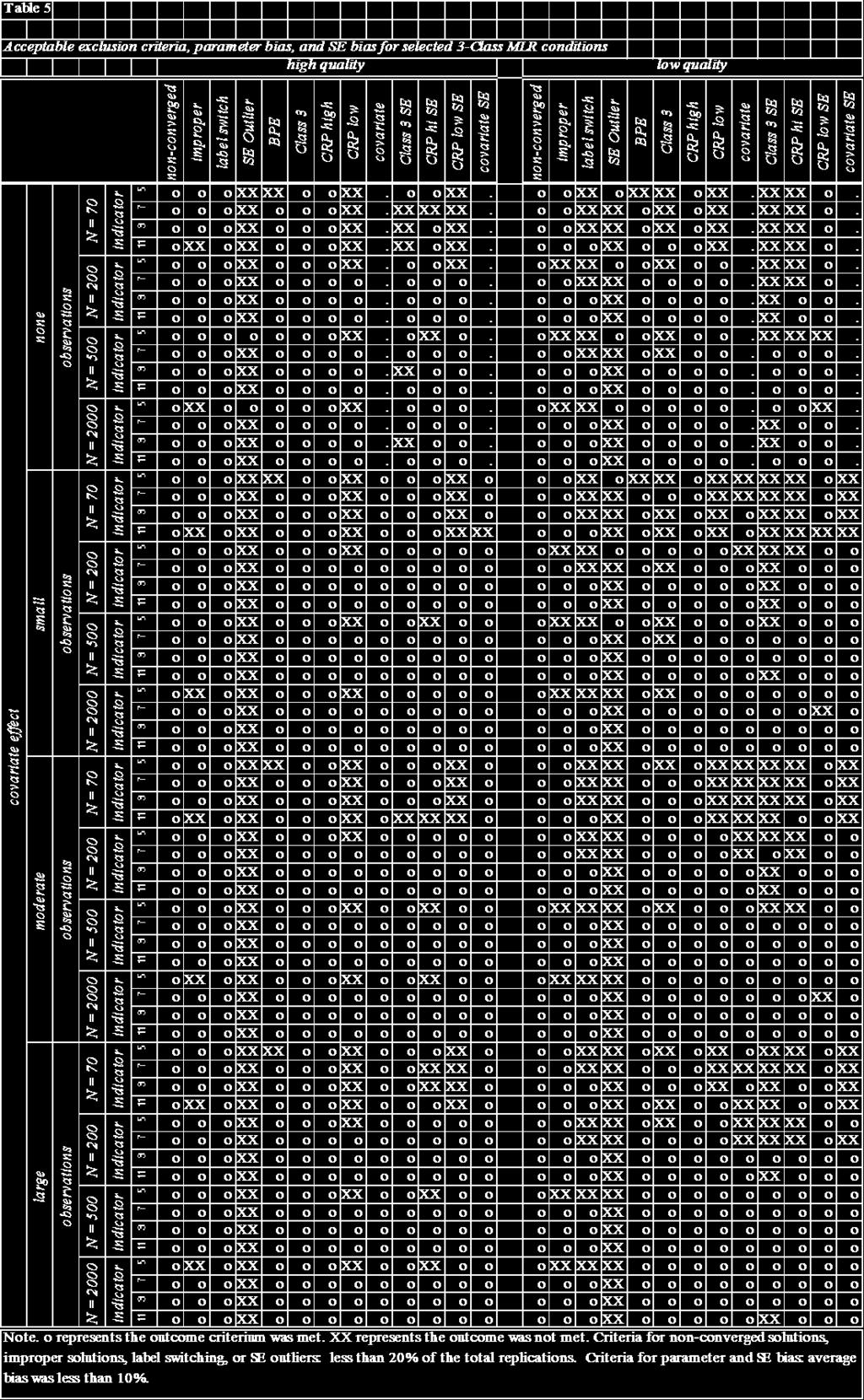
69 62

70 63

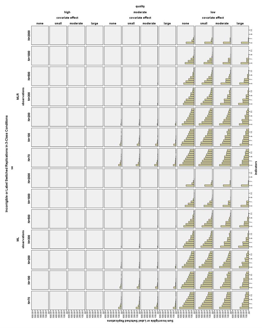
71 64

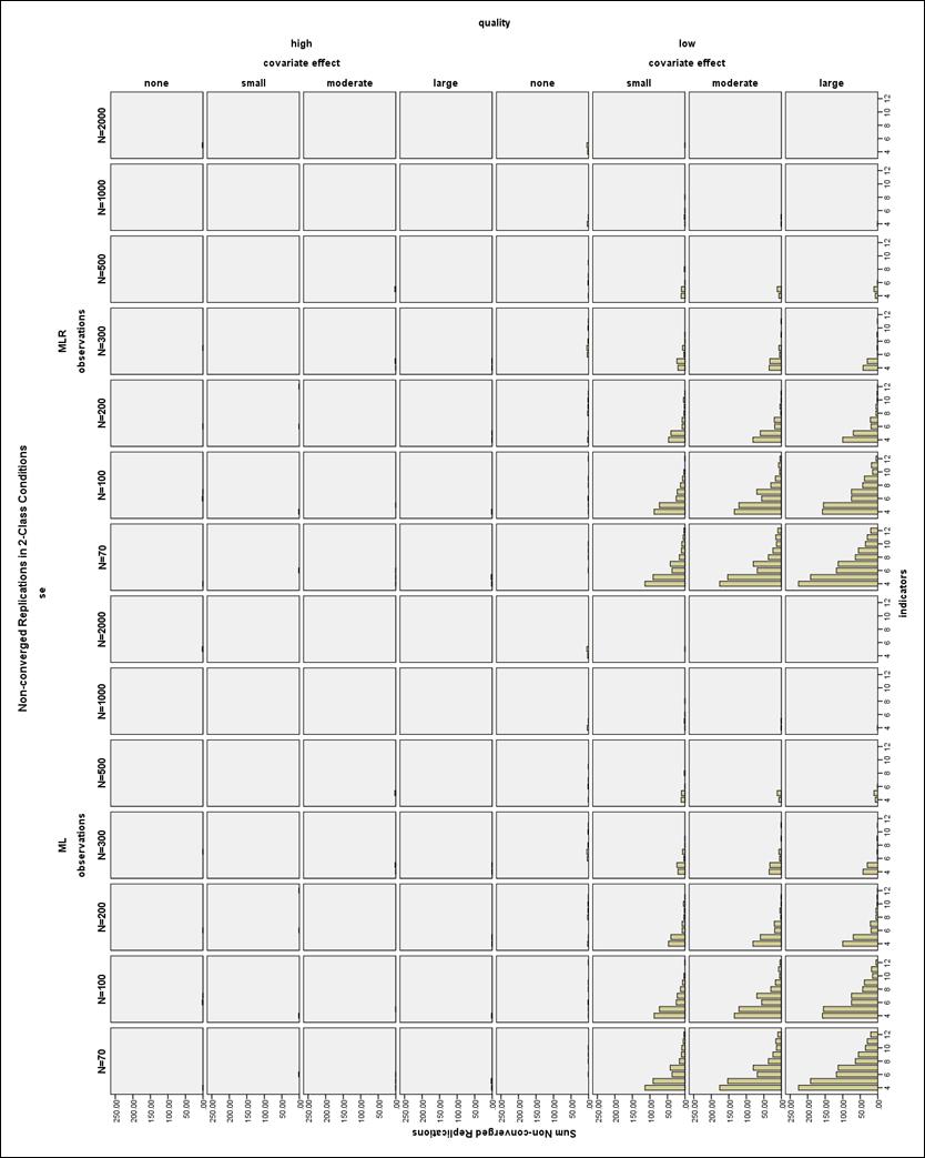
72 65

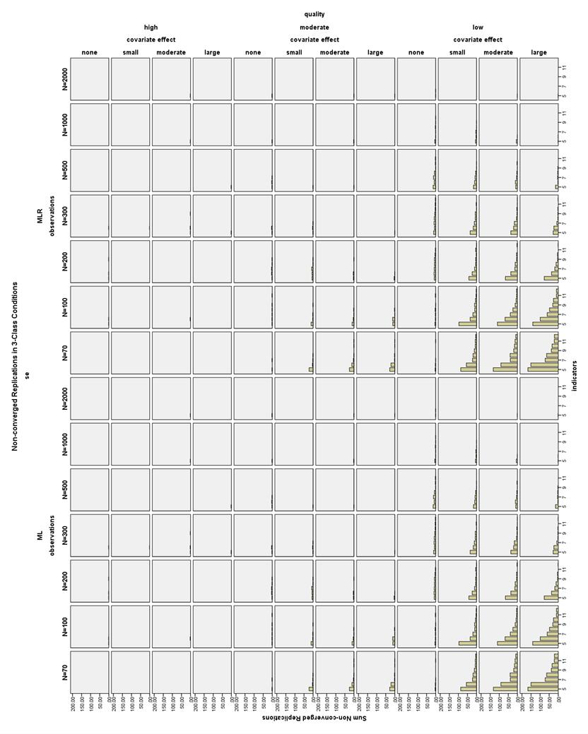
73 66

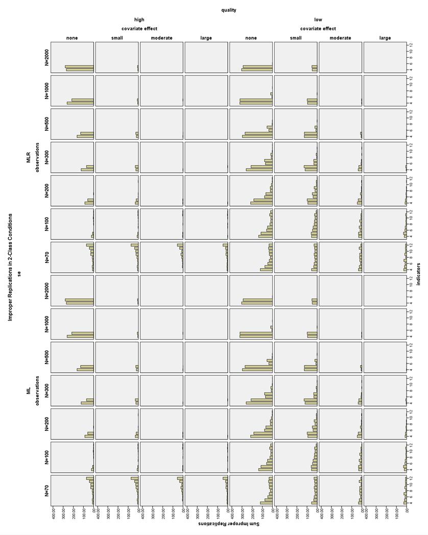
74 67

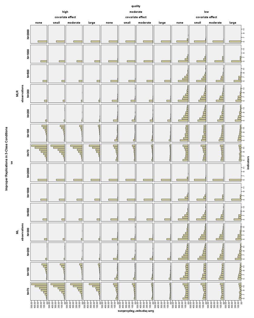
75 68

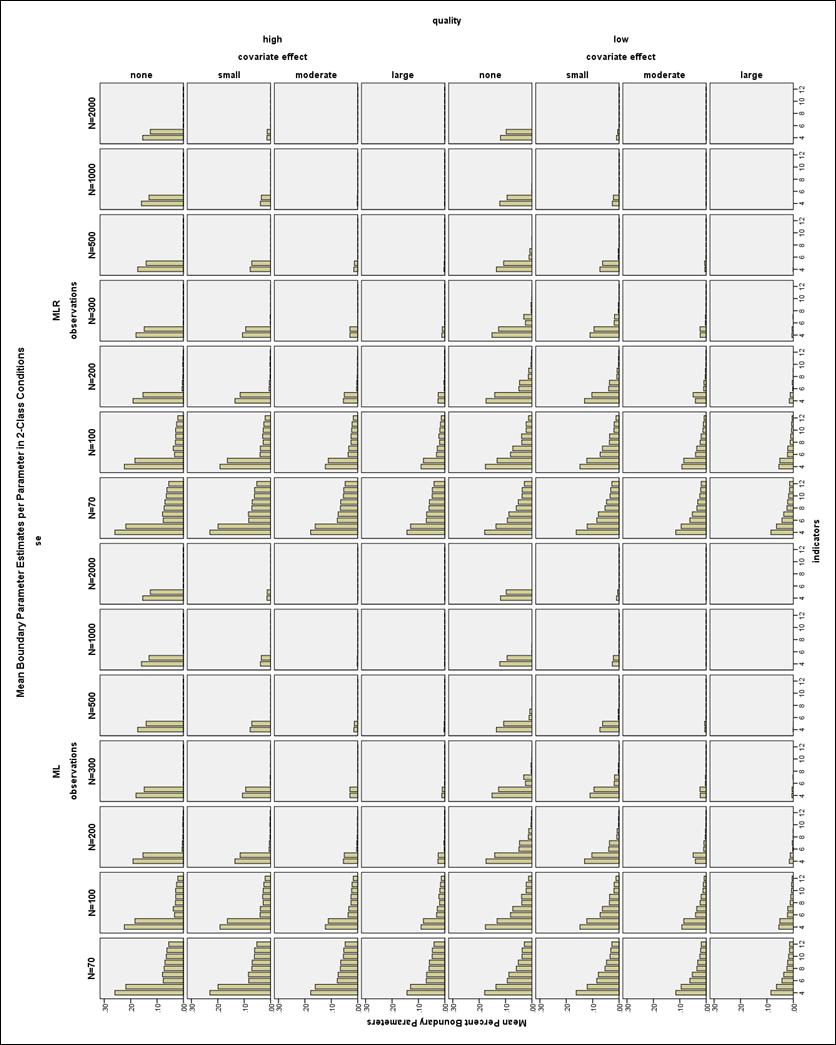
76 69

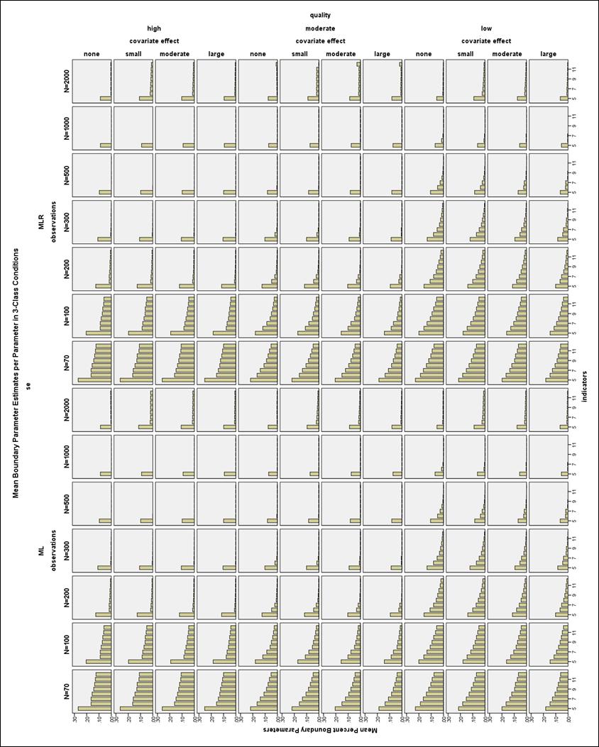
77 70

78 Figure 9. Covariate SE in 3-Class ML low quality conditions. 71

79 Figure 10. Covariate SE in 3-Class ML low quality conditions, outliers excluded. 72

80 73

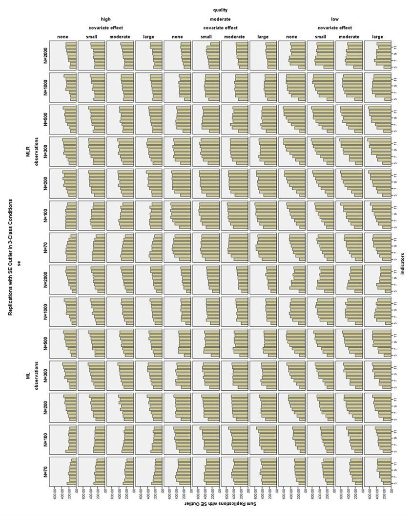
81 74

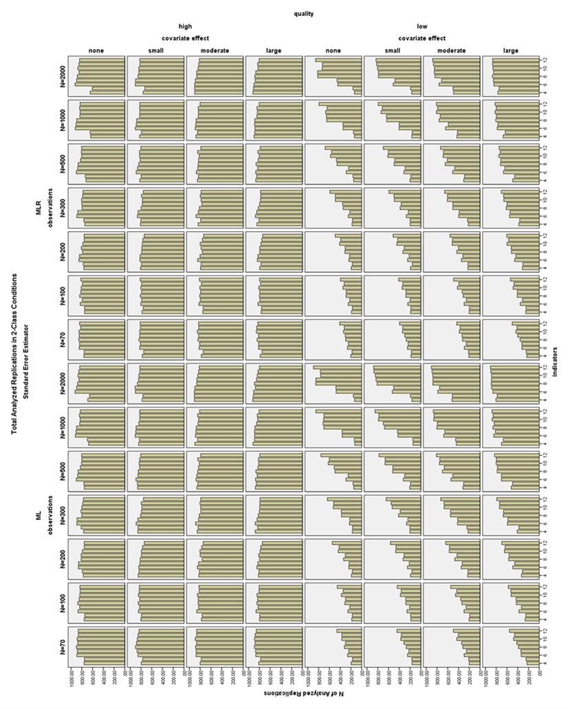
82 75

83 76

84 77

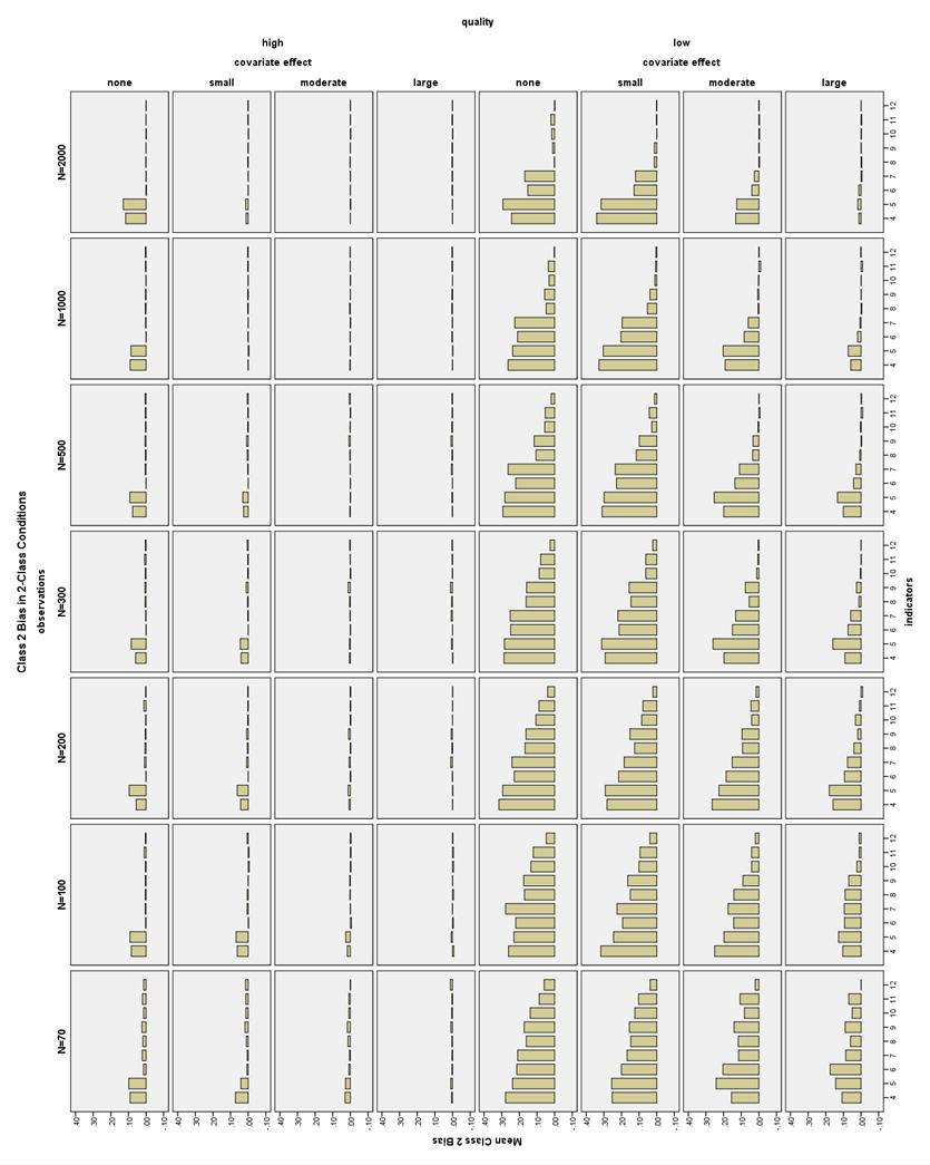
85 78

86 79

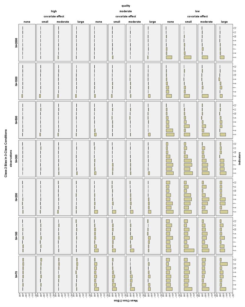
87 80

88 81

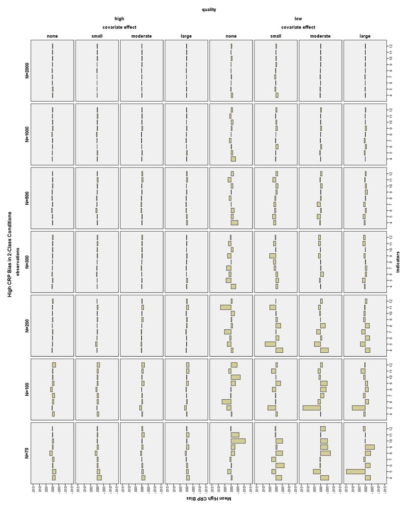
89 82

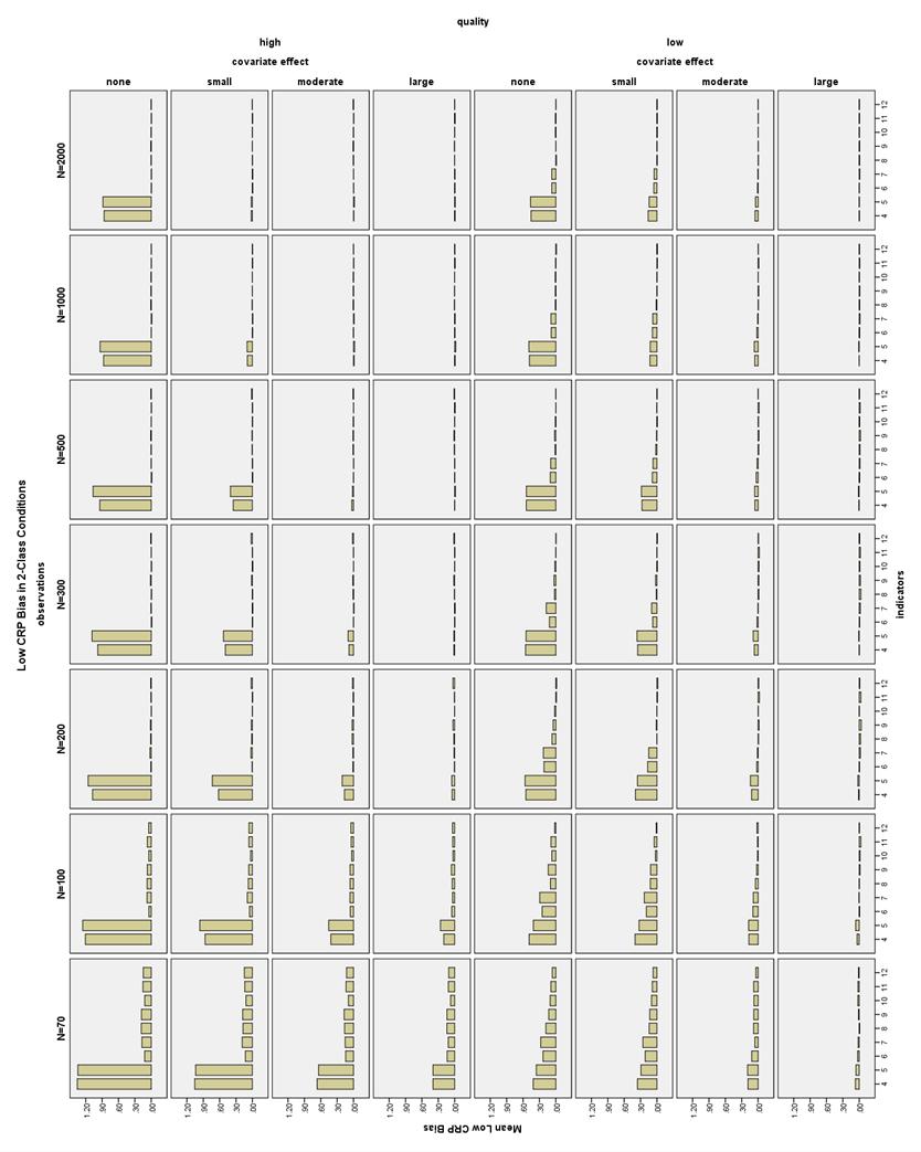
90 83

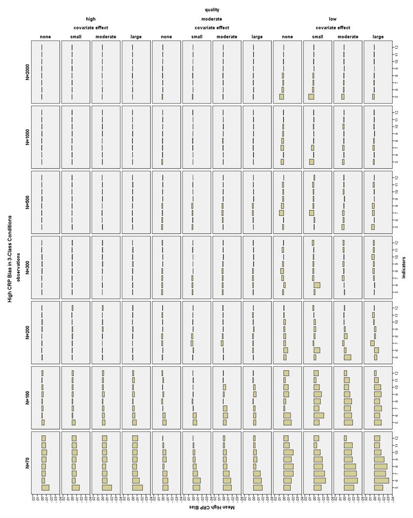
91 84

92 85

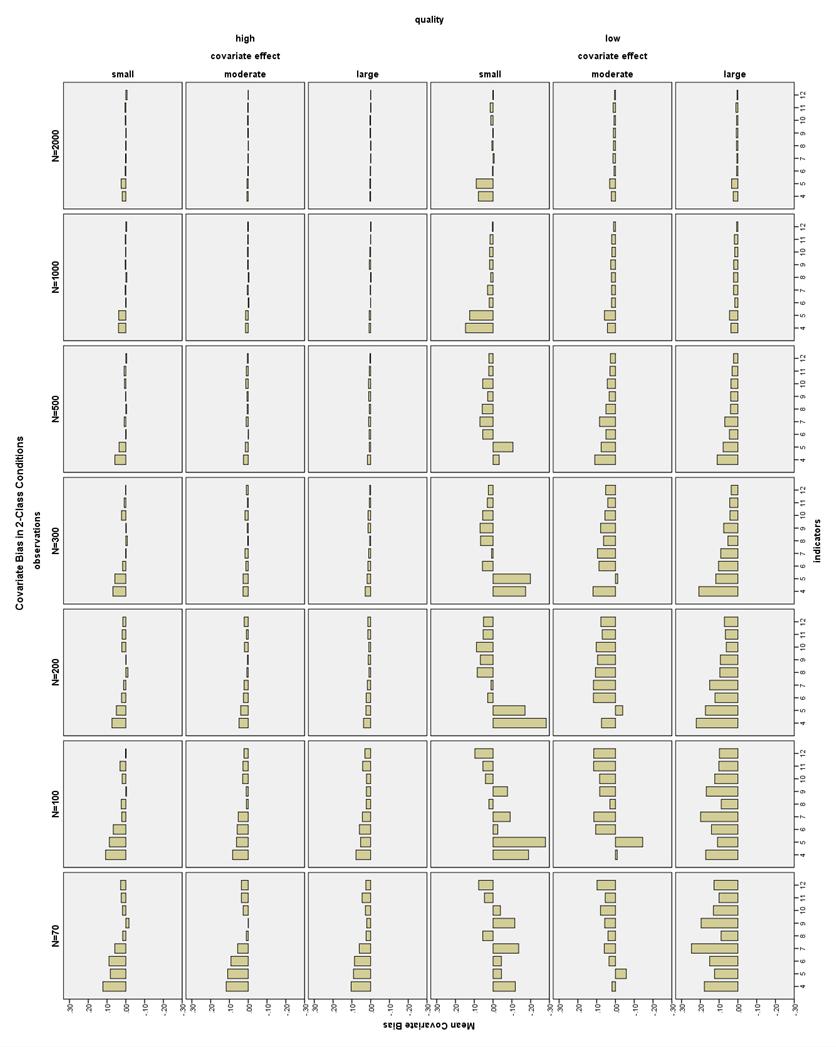
93 86

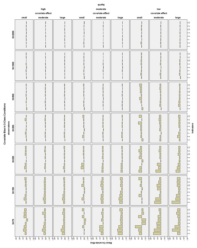
94 87

95 88

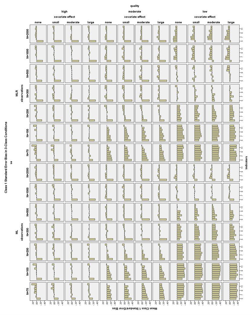
96 89

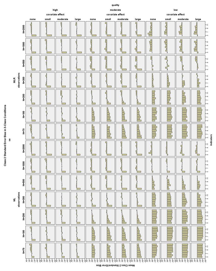
97 90

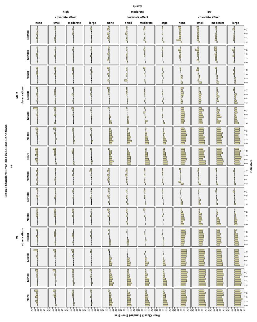
98 91

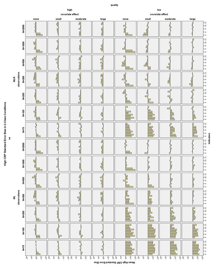
99 92

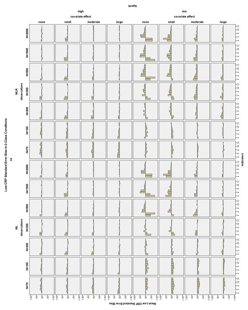
100 93

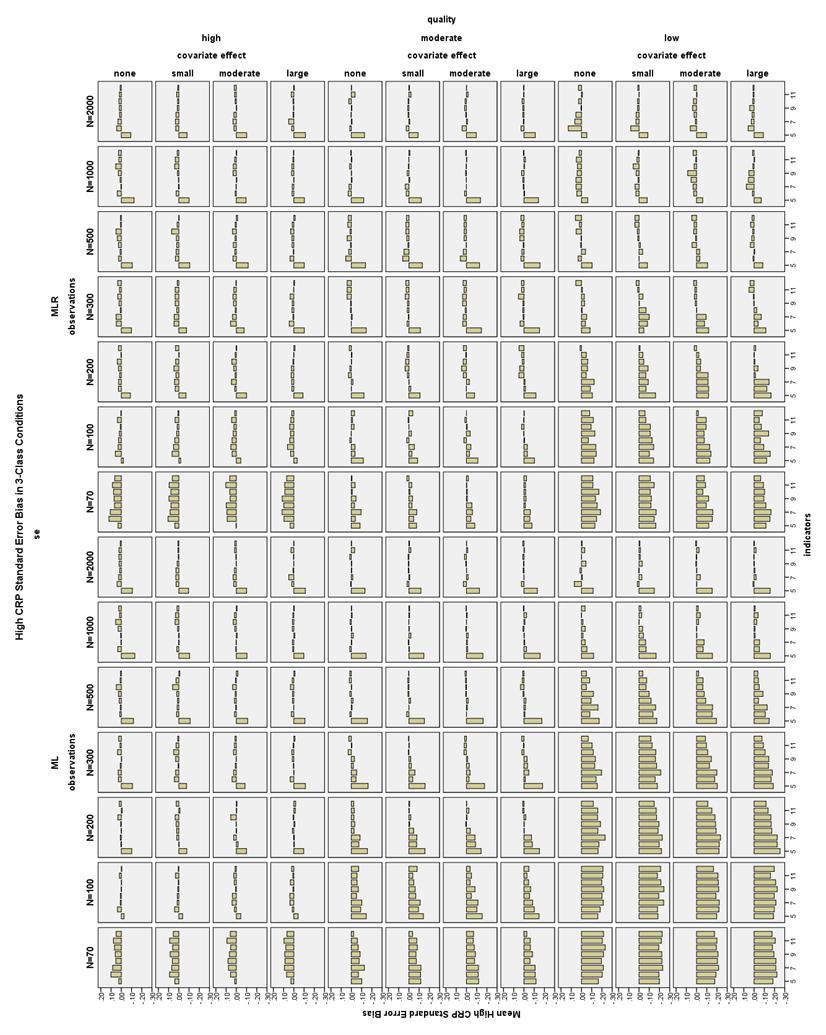
101 94

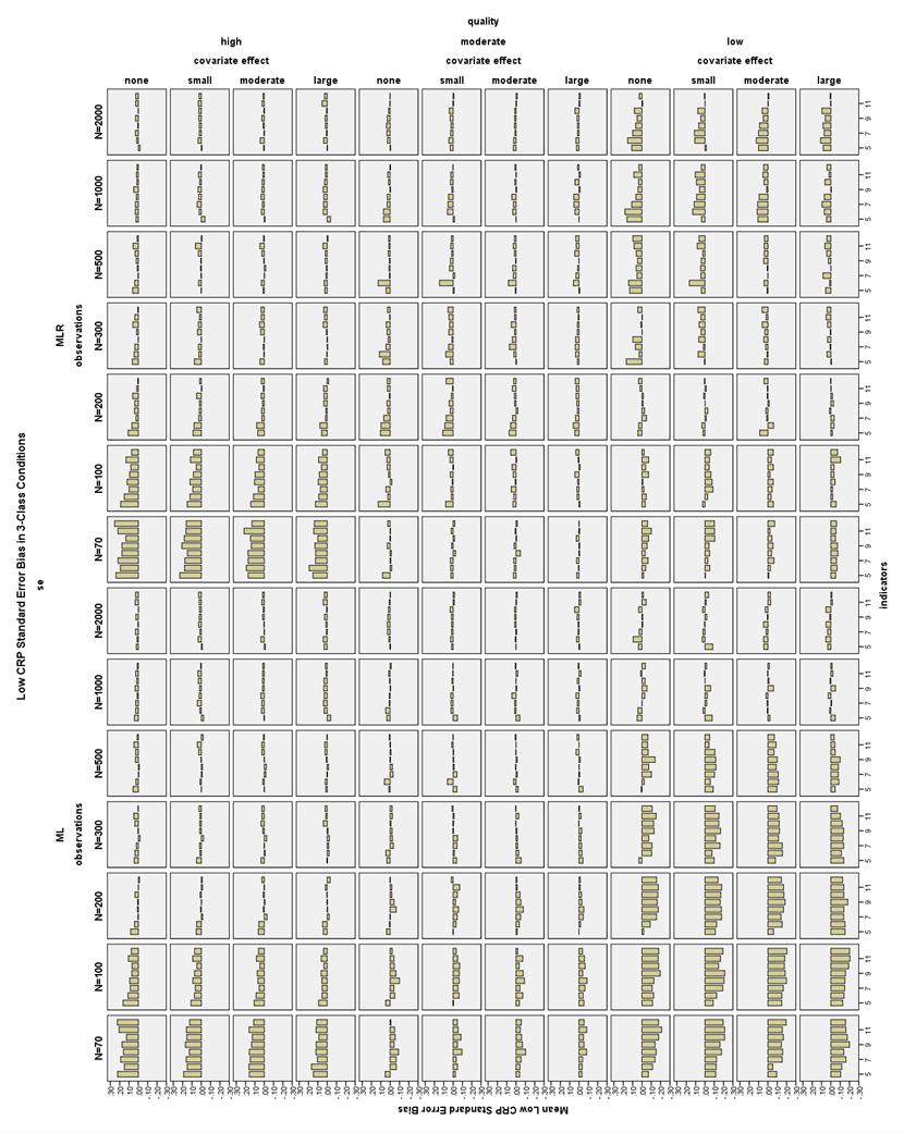
102 95

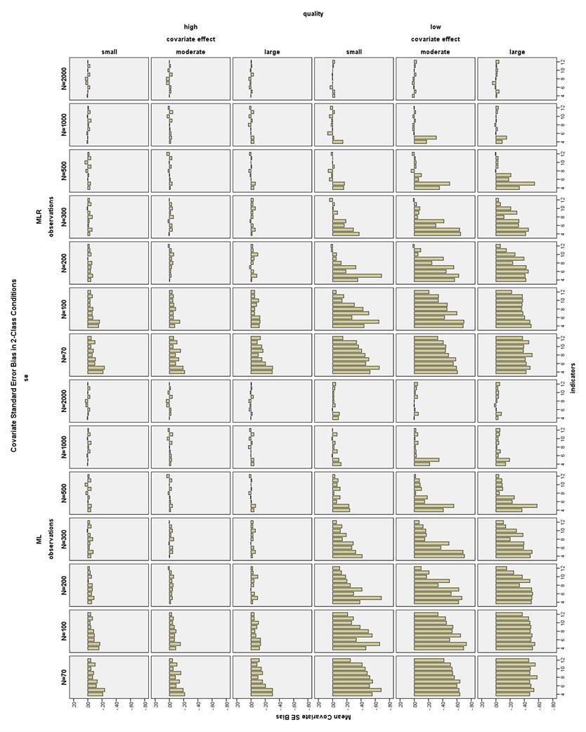
103 96

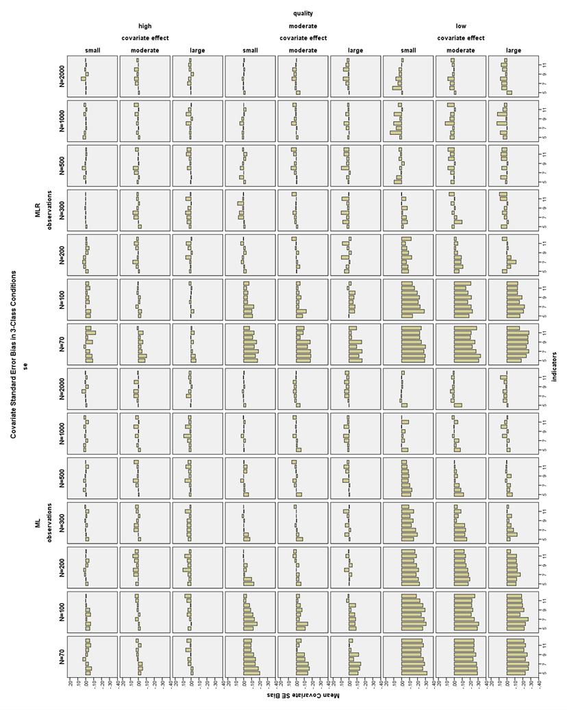
104 97

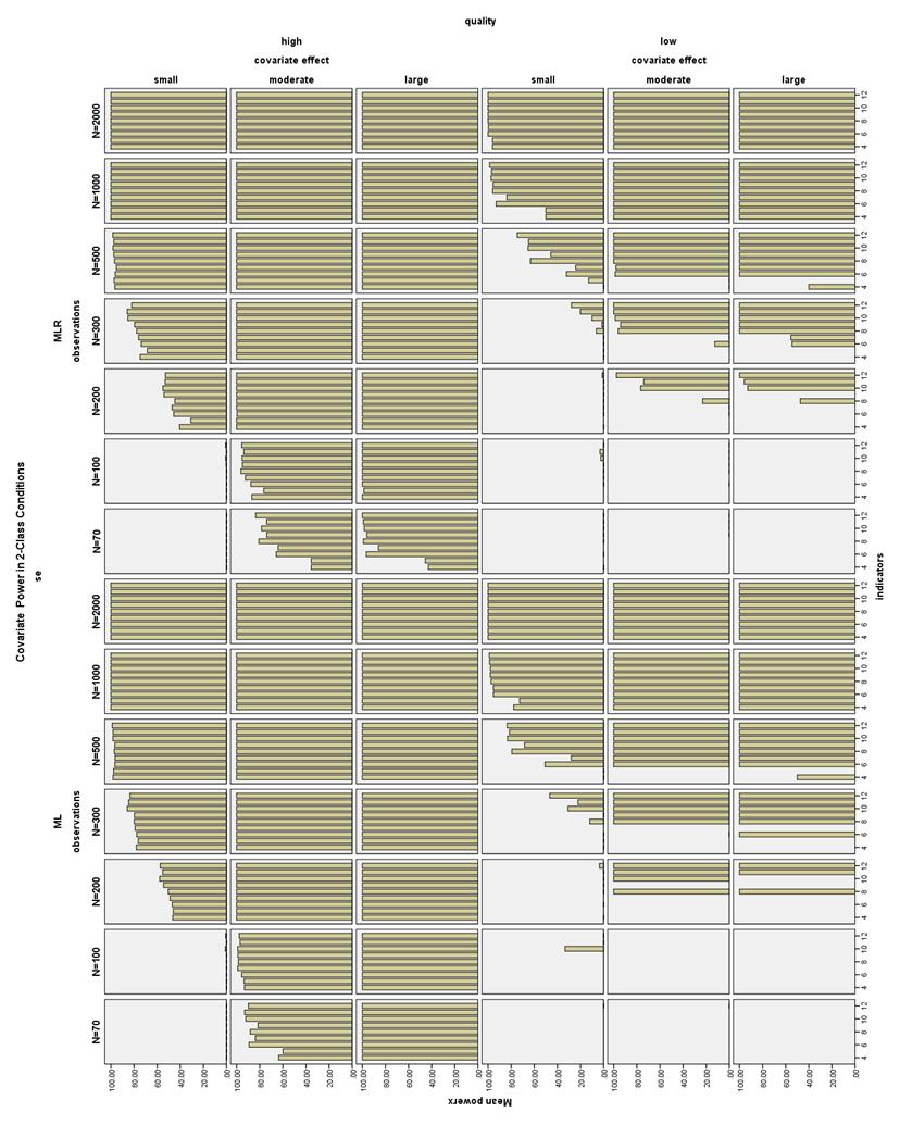
105 98

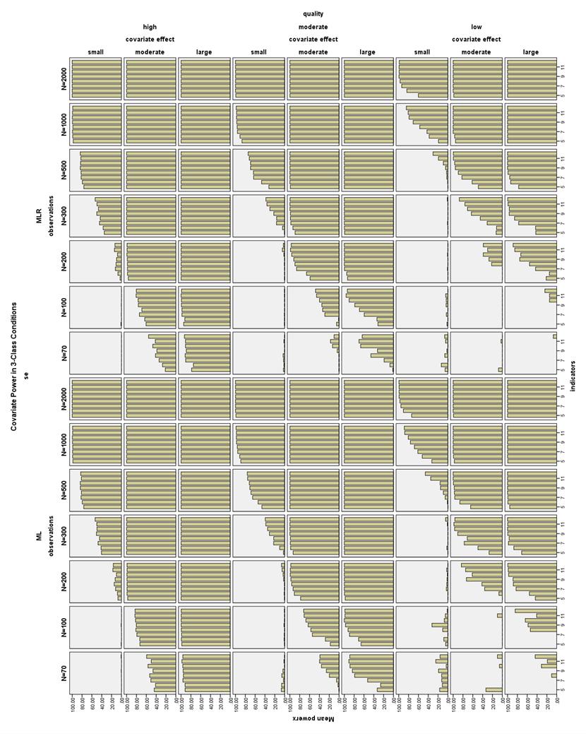
106 99

107 100

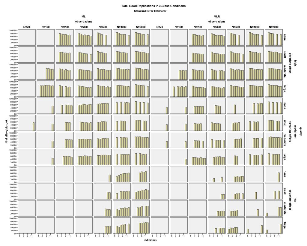
108 101