NMR Oil Well Logging: Diffusional Coupling and Internal Gradients in Porous Media. Vivek Anand

Transcription

1 RICE UNIVERSITY NMR Oil Well Logging: Diffusional Coupling and Internal Gradients in Porous Media by Vivek Anand A THESIS SUBMITTED IN PARTIAL FULFILLMENT OF THE REQUIREMENTS FOR THE DEGREE Doctor of Philosophy APPROVED, THESIS COMMITTEE George J. Hirasaki, A. J. Hartsook Professor, Chair Chemical and Biomolecular Engineering Walter G. Chapman, William W. Akers Chair, Chemical and Biomolecular Engineering Andreas Luttge, Associate Professor Earth Science and Chemistry HOUSTON, TEXAS APRIL 2007 i

2 ii ABSTRACT NMR Oil Well Logging: Diffusional Coupling and Internal Gradients in Porous Media by Vivek Anand The default assumptions used for interpreting NMR measurements with reservoir rocks fail for many sandstone and carbonate formations. This study provides quantitative understanding of the mechanisms governing NMR relaxation of formation fluids for two important cases in which default assumptions are not valid. The first is diffusional coupling between micro and macropore, the second is susceptibility-induced magnetic field inhomogeneties. Understanding of governing mechanisms can aid in better estimation of formation properties such as pore size distribution and irreducible water saturation. The assumption of direct correspondence between relaxation time and pore size distribution of a rock fails if fluid in different sized pores is coupled by diffusion. Pore scale simulations of relaxation in coupled micro and macropores are done to analyze the effect of governing parameters such as surface relaxivity, pore geometry and fluid diffusivity. A new coupling parameter () is introduced which quantifies the extent of coupling by comparing the rate of relaxation in a coupled pore to the rate of diffusional transport. Depending on, the pores can communicate through total, intermediate or

3 iii decoupled regimes of coupling. This work also develops a new technique for accurate estimation of irreducible saturation, an approach that is applicable in all coupling regimes. The theory is validated for representative cases of sandstone and carbonate formations. Another assumption used in NMR formation evaluation is that the magnetic field distribution corresponds to the externally applied field. However, strong field inhomogenities can be induced in the presence of paramagnetic minerals such as iron on pore surfaces of sedimentary rocks. A generalized relaxation theory is proposed which identifies three asymptotic relaxation regimes of motionally averaging, localization and free diffusion. The relaxation characteristics of the asymptotic regimes such as T 1 /T 2 ratio and echo spacing dependence are quantitatively illustrated by random walk simulations and experiments with paramagnetic particles of several sizes. The theory can aid in better interpretation of diffusion measurements in porous media as well as imaging experiments in Magnetic Resonance Imaging (MRI).

4 iv ACKNOWLEDGEMENTS First and foremost, I would like to acknowledge my advisor Dr. George J. Hirasaki for his continuous support and inspiration. I will remain indebted to him throughout my life for the things he has taught me. I would also like to thank Dr. Walter G. Chapman and Dr. Andreas Luttge for serving on my thesis committee. I am very thankful to William Knowles, Jie Yu and Shyam Benegal for their help with the BET, DLS and Coulter Counter measurements. I am also thankful to Dr. Vicki L. Colvin s Lab for providing magnetite nanoparticles and TEM measurements. Many thanks go to Jim Howard at Conoco Phillips for proving North Burbank cores and Chuck Devier at PTS labs for making mercury porosimetry and permeability measurements. I greatly appreciate Dr. Marc Fluery at French Institute of Petroleum (IFP) for sharing his carbonate NMR measurements at high temperatures. I would like to acknowledge Department of Energy (grant number DE-PS26-04NT15515) and consortium for processes in porous media for the financial support. Most importantly, I would like to thank my parents, my family members for their love and support.

5 v TABLE OF CONTENTS TITLE PAGE i ABSTRACT ii ACKNOWLEDGEMENTS...iv TABLE OF CONTENTS.v LIST OF TABLES..ix LIST OF FIGURES...xi Chapter 1. Introduction...1 Chapter 2. Diffusional Coupling Literature Review Nuclear Magnetism Pulse tipping and Free Induction Decay Longitudinal relaxation Transverse relaxation NMR formation evaluation Diffusional coupling Spectral BVI and tapered T 2,cutoff Diffusional coupling between micro and macropore Mathematical modeling Magnetization decay in coupled pore Coupling Parameter Micropore relaxation Macropore relaxation Estimation of irreducible saturation and Unification of spectral and sharp T 2,cutoff theory Diffusional coupling between pore lining clays and pore body Pore size distribution of North Burbank sandstone...32

6 vi Numerical solution of Bloch equation in pore size distribution Simulated T 2 distributions Coupling regimes in North Burbank sandstone Estimation of surface relaxivity Effect of clay distribution on diffusional coupling Synthesis of model shaly sands with laminated and dispersed clays T 2 distribution of shaly sands Estimation of irreducible water saturation in shaly sands Diffusional coupling in microporous grainstones Coupling parameter for grainstones Experimental validation of grain size dependence on pore coupling Estimation of irreducible saturation for the sandstone and grainstone systems Effect of temperature on diffusional coupling Temperature dependence of Temperature dependence of T 2 distributions of silica gels and carbonate core Discussion Conclusions 71 Chapter 3. Paramagnetic Relaxation in Sandstones: Generalized Relaxation Theory Introduction and Literature Review Generalized secular relaxation theory Characteristic time scales for secular relaxation Characteristic time scale for restricted diffusion in a constant gradient Characteristic time scale for relaxation in field induced by paramagnetic sphere Asymptotic regimes of secular relaxation Motionally averaging regime Free diffusion regime...83

7 vii Localization regime Parametric representation of asymptotic regimes Relaxation regimes in sedimentary rocks Paramagnetic particles at dilute surface concentration Paramagnetic particles at high surface concentration Random walk simulations Non-dimensionalization of Bloch equations Algorithm Validation of numerical solution Unrestricted diffusion in constant gradient Restricted diffusion in constant gradient Results Conclusions..117 Chapter 4. Paramagnetic Relaxation in Sandstones: Experiments Paramagnetic particles in aqueous dispersions Ferric Ion Polymer coated magnetite nanoparticles Magnetite nanoparticles coated with citrate ion Characteristic time scales for paramagnetic particles in dispersion Paramagnetic particles on silica surface Fine sand coated with ferric ions Fine sand coated with magnetite nanoparticles Fine sand with dispersed 2.4 m magnetite Coarse sand coated with magnetite nanoparticles Paramagnetic relaxation in sandstones Motionally averaging regime Free diffusion regime Localization regime Parametric representation of asymptotic regimes in experimental systems Conclusions..159

8 viii Chapter 5. Conclusions 161 Chapter 6. Future Work..166 REFERENCES Appendix A. Numerical solution of Bloch equations in coupled pore model 174 Appendix B. Relaxation time of micropore in coupled pore model Appendix C. Characteristic parameters for the sandstones and grainstone systems..185 Appendix D. Characteristic parameters for the experimental systems of Chapter

9 ix LIST OF TABLES Table 2.1: Characteristic parameters for the simulations for three NB cores 39 Table 2.2: Physical Properties of Fine Sand, Kaolinite and Bentonite clays.44 Table 2.3: Physical properties of the grainstone systems..55 Table 4.1: Characteristic Time scales for the ferric ions and magnetite nanoparticles Table 4.2: Longitudinal and transverse relaxation times of water-saturated fine sand coated with ferric ions at different surface concentrations (area/ferric ion) Table 4.3: Longitudinal and transverse relaxation times of water-saturated fine sand coated with 25 nm magnetite at different surface concentrations 137 Table 4.4: Longitudinal and transverse relaxation times of water-saturated fine sand coated with 110 nm magnetite at different surface concentrations Table 4.5: Longitudinal and transverse relaxation times of water-saturated fine sand with dispersed 2.4 m magnetite Table 4.6: Longitudinal and transverse relaxation times of water-saturated coarse sand coated with 25 nm magnetite at different surface concentrations 144 Table 4.7: Characteristic time scales for relaxation in coarse sand coated with 25nm 2 ( 710 nm 2 6 /particle) and fine sand coated with 110nm magnetite ( nm 2 /particle) Table 4.8: Characteristic time scales for relaxation in fine sand coated with 25 nm and 110 nm magnetite at high surface concentrations Table 4.9: Characteristic time scales for relaxation in fine with dispersed 2.4 µm magnetite Table 4.10: Logmean longitudinal and transverse relaxation times of water saturated North Burbank cores 151 Table A.1: Model parameters for magnetization decay simulations Table C.1: Characteristic parameters for North Burbank sandstone..185 Table C.2: Characteristic parameters for chalk 185 Table C.3: Characteristic parameters for silica gels 185

10 x Table C.4: Characteristic parameters for molecular sieves.186 Table C.5: Characteristic parameters for silica gels at 30, 50, 75 and 95 o C Table C.6: Characteristic parameters for reservoir carbonate core at 25, 50, 80 o C.186 Table D.1: Characteristic parameters for fine sand coated with 25 nm magnetite at D different surface concentrations. and 1 T are dimensionless ,sec Table D.2: Characteristic parameters for fine sand coated with 110 nm magnetite at D different surface concentrations. and 1 T are dimensionless ,sec Table D.3: Characteristic parameters for coarse sand coated with 25 nm magnetite at D different surface concentrations. and 1 T are dimensionless ,sec Table D.4: Characteristic parameters for fine sand with dispersed 2.4m magnetite at D different concentrations. and 1 T are dimensionless ,sec Table D.5: Characteristic parameters for North-Burbank sandstones. and 1 T dimensionless D 2,sec are

11 xi LIST OF FIGURES Figure 2.1: Conceptual model of pore coupling in clay-lined pores in sandstones (Straley et al., 1995) (a) at 100% water saturation (b) at irreducible saturation.12 Figure 2.2: Physical model of coupled pore geometry. Fluid molecules relax at the micropore surface while diffusing between micro and macropore 14 Figure 2.3: Contour plots of magnetization at t =1 in coupled pores with = 0.5 and = 10 and different values of. The gradients along the longitudinal direction for larger imply that micropore is relaxing faster compared to macropore...18 Figure 2.4: Contour plots of magnetization at t =1 in coupled pores with = 0.5 and = 0.1 and different values of. For comparison, the aspect ratios are not drawn to scale. Note the difference in contour plots for systems with same...19 Figure 2.5: Simulated T 2 distributions of coupled pores with = 0.5 and = 10 and different values of. The systems transition from unimodal to bimodal distribution with increase in..21 Figure 2.6: Simulated T 2 distributions of coupled pores with = 0.5 and = 0.1 and different values of. The T 2 distributions transition from unimodal to bimodal distribution with increase in even though µ remains same 22 Figure 2.7: Plot of independent microporosity fraction (/β) with for different simulation parameters. The inset shows plot of (/β) with for same simulation parameters..24 Figure 2.8: Plot of dimensionless relaxation time of macropore with (1 ).26 Figure 2.9: Contour plots of correlations for and T 2,macro /T 2,µ in the and parameter space...28 Figure 2.10: Plot of vs. T 2,macro /T 2,µ for different. A spectral or tapered cutoff is required for the estimation of irreducible saturation in the intermediate coupling regime. A sharp cutoff is applicable for decoupled regime 30 Figure 2.11: (a) Model of a clay-lined pore showing micropores opening to a macropore (Straley et al., 1995) (b) Simplified model with rectangular clays arranged along macropore wall Figure 2.12: Pore throat distribution of the North Burbank sandstone obtained from mercury porosimetry. The bimodal distribution arises due to pore-lining chlorite... 32

12 xii Figure 2.13: Lognormal pore size distribution simulated to approximate the distribution of macropores. Also shown are the pores with changing proportion of pore volume occupied by the clay flakes Figure 2.14: Simulated T 2 distributions for c = 0.3 and c = 100 showing transition from unimodal to bimodal distribution with increase in...37 Figure 2.15: Comparison of simulated and experimental T 1 distributions for three water saturated North Burbank cores Figure 2.16: (a) Independent microporosity fraction agrees with the lognormal relationship (Equation 2.25) for the three North Burbank cores (b) Normalized macropore relaxation time also agrees with the cubic relationship (Equation 2.27)...40 Figure 2.17: Comparison of simulated and experimental distributions for two hexane saturated North Burbank cores...41 Figure 2.18: T 2 distributions of dispersed kaolinite-sand systems for different clay weight fractions. 46 Figure 2.19: T 2 distributions of laminated kaolinite-sand systems for different clay weight fractions.46 Figure 2.20: T 2 distributions of dispersed bentonite-sand systems for different clay weight fractions..47 Figure 2.21: T 2 distributions of laminated bentonite-sand systems for different clay weight fractions..47 Figure 2.22: Linear dependence of the relaxation rates of dispersed clay-sand systems with the clay content..48 Figure 2.23: Comparison of the irreducible water saturation calculated using the inversion technique and measured experimentally for dispersed systems 51 Figure 2.24: Pore coupling model in grainstone systems. The three-dimensional model (Ramakrishan et al., 1999) can be mapped to a two-dimensional model of periodic array of microporous grains separated by macropores...52 Figure 2.25: T 2 distributions of microporous chalk as a function of grain radius. The transition from decoupled (R g = 335 m) to total coupling regime (R g = 11 m) is predicted by the values of Figure 2.26: T 2 distributions of silica gels as a function of grain radius. The transition from almost decoupled (R g = 168 m) to total coupling regime (R g = 28 m) is predicted by the values of...59

13 xiii Figure 2.27: T 2 distributions of alumino-silicate molecular sieves as a function of grain radius.60 Figure 2.28: The lognormal and cubic relationships of Equations (2.25) and (2.27) hold for the grainstone systems.61 Figure 2.29: Comparison of calculated and experimentally measured values of microporsoity fraction () for the grainstone and sandstone systems. The values are estimated within 4% average absolute error..62 Figure 2.30: Comparison of calculated and experimentally measured values of for the grainstone and sandstone systems. The values are estimated within 11% error for all coupling regimes Figure 2.31: T 2 distributions of silica gels at 100% water saturation and at 30, 50, 75 and 95 o C...66 Figure 2.32: T 2 distribution of medium coarse silica gel at irreducible saturation and at 30, 50, 75 and 95 o C...66 Figure 2.33: T 2 distributions of the Thamama formation carbonate core at 100% water (upper panel) and irreducible water saturation (lower panel) at 25, 50 and 80 o C (Fleury, 2006).69 Figure 2.34: Plot of independent microporosity fraction (/) with for grainstone systems and carbonate core Figure 2.35: Comparison of the microporosity fraction calculated using the inversion technique and measured experimentally for silica gels and carbonate core..71 Figure 3.1: Magnetic field lines in the presence of a paramagnetic sphere with magnetic susceptibility 10 6 times that of the surrounding medium. The field lines concentrate in their passage through the sphere 76 Figure 3.2: Contour plots of z component of internal magnetic field (dimensionless) induced by a unit paramagnetic sphere in a vertical plane passing through the center of the sphere. The external magnetic field is applied in the vertical z direction Figure 3.3: Schematic diagram of asymptotic relaxation regimes in ( R, E ) parameter space..88 Figure 3.4: (a) Contour plots of dimensionless magnetic field (Equation 3.12) in the outer region of a silica grain coated with paramagnetic spheres at dilute concentrations(no. of particles per unit area ~ 3). Radial distance is normalized with respect to the radius of the grain. The ratio of radius of the silica grain to that of paramagnetic particles is 10. (b) Contour plots in a quadrant at higher magnification

14 xiv Figure 3.5: (a) Contour plots of dimensionless magnetic field (Equation 3.12) in the outer region of a silica grain coated with paramagnetic spheres at high concentrations (No. of particles per unit area ~ 30). Radial distance is normalized with respect to the radius of the grain. The ratio of radius of the silica grain to that of paramagnetic particles is 10. (b) Contour plots in a quadrant at higher magnification.93 Figure 3.6: Contour plots of dimensionless magnetic field (Equation 3.12) in the outer region of a paramagnetic shell around a unit sphere. The thickness of the shell is calculated such the volume of the shell is same as the total volume of paramagnetic particles in Figure Figure 3.7 Schematic diagram of a tetrahedral pore between four touching silica grains of radius R g. The length scale of field inhomogeneity is equal to the dimension of the tetrahedral pore when the paramagnetic particles are present at high concentration on the surface of the grains...96 Figure 3.8: Comparison of analytical and simulated echo decay for unrestricted diffusion in a constant gradient. The parameters used in the simulations are g = 100 G/cm, E = 2 ms, N w = 10,000 and dt = 0.1 µs. The simulated echo decay matches within 0.1% of the analytical decay 102 Figure 3.9: Comparison of simulated and analytical echo decays for restricted diffusion in a sphere with a constant gradient. The parameters used in the simulations are L g * = 1.2 and L d * = 2 (upper panel) and L d * = 3 (lower panel). Lesser number of points in the lower figure is due to smaller sampling rate with larger L d *. The analytical rate is given by Equation (3.54) normalized by 1/t c Figure 3.10: Comparison of simulated and analytical echo decays for restricted diffusion in a sphere with a constant gradient. The parameters used in the simulations are L g * = 1.5 and L d * = 2 (upper panel) and L d * = 3 (lower panel). Lesser number of points in the lower figure is due to smaller sampling rate with larger L d *. The analytical rate is given by Equation (3.54) normalized by 1/t c Figure 3.11: Plot of simulated secular relaxation rate (dimensionless) with R as a -4 function of E. The parameters used in the simulations are = , k = 1.2, B 0 = 496 Gauss. The solid, dotted and dash-dotted line are the theoretically estimated secular relaxation rates according to the outer sphere theory (Equation 3.60), mean gradient diffusion theory (Equation 3.61) and modified mean gradient diffusion theory (Equation 3.62) plotted in the respective regimes of validity. The dashed lines are the boundaries R = 1 and E = 1 that delineate the asymptotic regimes.107 Figure 3.12: Contour plots of dimensionless secular relaxation rate in the ( R, E ) parameter space. Contours differ by a factor of 10. The parameters used in the -4 simulations are = , k = 1.2, B 0 = 496 Gauss. The dotted lines are the

15 xv corresponding plots for the theoretically predicted relaxation rates given by Equations (3.60), (3.61) and (3.62). The bold dashed lines are the boundaries between asymptotic -4 regimes. The contours are invariant for dilute volume fractions ( ).112 Figure 3.13: Plot of secular relaxation rates (dimensionless) with dimensionless echo -4 spacing E for R 1. The parameters used in the simulations are = , k = 1.2, B 0 = 496 Gauss. The dotted lines are the plots of theoretically predicted relaxation rates in the motionally averaging regime given by Equation (3.60). The bold dashed line is the boundary E = R delineating free diffusion and motionally averaging regimes. The relaxation rates are almost independent of the echo spacing in the motionally averaging regime Figure 3.14: Plot of secular relaxation rates (dimensionless) with dimensionless echo -4 spacing E for R >>1. The parameters used in the simulations are = , k = 1.2, B 0 = 496 Gauss. The dotted and dash-dotted lines are the theoretically predicted relaxation rates in the free diffusion and the localization regime given by Equations (3.61) and (3.62) respectively. The bold dashed line is the boundary E =1 delineating free diffusion and localization regimes. The dependence of the relaxation rates on echo spacing is less than quadratic in the localization regime.114 Figure 3.15: Contour plots of dimensionless secular relaxation rate in the ( R, E ) parameter space for = 0.6. A paramagnetic shell with susceptibility 0.2 (SI units) and 3ε/R g = 10-3 is assumed for the simulations. Contours differ by a factor of 10. The dotted lines are the corresponding plots for the theoretical relaxation rates given by Equations (3.60), (3.61) and (3.62). The bold dashed lines are the boundaries between asymptotic regimes..116 Figure 3.16: Plot of average absolute deviation (%) of simulations with higher volume fractions from the simulations with = The deviation is less than 10% for < Figure 4.1: Longitudinal and Transverse relaxation rates ( E = 0.2 ms) of ferric chloride solutions as a function of the concentration of the solution. No echo spacing dependence of T 2 relaxation was observed and T 1 /T 2 ratio is equal to unity Figure 4.2: TEM images of magnetite nanoparticles. (a) 4 nm magnetite (b) 9 nm magnetite (c) 16 nm magnetite (Agarwal, 2007). 122 Figure 4.3: Plots of transverse, longitudinal and secular relaxation rates with the concentration of aqueous dispersions of polymer-coated nanoparticles of three different sizes. The average diameter of the nanoparticles (D p ) and slopes of the linear best fits are also mentioned

16 xvi Figure 4.4: T 1 and T 2 distributions of aqueous dispersions of ferric ions and polymer coated magnetite nanoparticles. The T 2 distributions are independent of the echo spacing and T 1 / T 2 ratio increases with the particle size Figure 4.5: T 1 /T 2 ratio of the aqueous dispersions of paramagnetic particles as a function of the particle size. The T 1 /T 2 ratio increases with the particle size in the motionally averaging regime..125 Figure 4.6: Particle size distribution of magnetite dispersions synthesized using Massart s method (1981). The average diameters of the particles are 25 nm (upper panel) and 110 nm (lower panel) respectively Figure 4.7: Plots of transverse, longitudinal and secular relaxation rates with the concentration of aqueous dispersions of magnetite nanoparticles synthesized using Massart s Method (1981). The average diameters of the nanoparticles (D p ) and slopes of the linear best fits are also mentioned Figure 4.8: T 1 and T 2 distributions of aqueous dispersions of ferric ions and citrate coated magnetite nanoparticles. The T 2 distributions are independent of the echo spacing and T 1 /T 2 ratio increases with the particle size Figure 4.9: T 1 and T 2 distributions of fine sand coated with ferric ions at different surface concentrations..135 Figure 4.10: T 1 and T 2 distribution of water-saturated fine sand coated with 25 nm magnetite nanoparticles at various concentrations..138 Figure 4.11: T 1 and T 2 distribution of water-saturated fine sand coated with 110 nm magnetite nanoparticles at various concentrations Figure 4.12: T 1 and T 2 distributions of fine sand with dispersed 2.4 m magnetite at two concentrations. A large T 1 / T 2 ratio and echo spacing dependence of transverse relaxation is observed Figure 4.13: T 1 and T 2 distributions of coarse sand coated with 25 nm magnetite at different surface concentrations Figure 4.14: Plot of the secular relaxation rate of water-saturated coated sand with E for cases in which free diffusion regime is observed. The surface concentrations are nm 2 2 /110 nm particle (fine sand) and 710 nm 2 /25 nm particle (coarse sand) respectively. The vertical lines are the boundary E = 1 at which the two systems transition from the free diffusion to the localization regime. The solid lines are the regression lines for the power-law fits in the two relaxation regimes. Relaxation rates show almost quadratic dependence on echo spacing in the free diffusion regime and less than linear dependence in the localization regime

17 xvii Figure 4.15: T 1 and T 2 distributions of water saturated North Burbank sandstone cores 1 and Figure 4.16: Plot of secular relaxation rate with half echo spacing for the several cases of the localization regime. The solid lines are the regression lines for the power law fits to the data. The exponents of the power law fits are less than unity for all cases Figure 4.17: Parametric representation of dimensionless secular relaxation rates for experimental systems in the ( R, E ) parameter space. The symbols are the experimental systems: (+) aqueous dispersion of 4nm, 9nm, 16nm particles, (*) fine and coarse sand coated with dilute concentrations of 25nm, ( ) fine sand coated with dilute surface concentration of 110nm magnetite, (Δ) fine sand coated with 25nm magnetite 3 Conc. = 710 nm 2 3 /part, ( ) fine sand coated with 25nm magnetite Conc. = 3 10 nm 2 2 /part., () coarse sand coated with 25nm magnetite Conc. = 7 10 nm 2 /part., ( ) fine 6 sand coated with 110nm magnetite Conc. = nm 2 /part., ( ) fine sand coated with 5 110nm magnetite Conc. = 310 nm 2 /part, () fine sand with dispersed 2.4µm magnetite, () North Burbank sandstone. (a) Comparison with contour plots for (b) Comparison with contours for = Figure 4.18: Plot of secular relaxation rates with E for experimental systems in free diffusion and localization regimes. The relaxation rates show nearly quadratic dependence on echo spacing in the free diffusion regime and less than linear dependence in the localization regime.158 Figure 4.19: T 1 /T 2 ratio for experimental systems. The ratio ranges from 1.1 to 13 and is echo spacing dependent for several systems Figure A.1: Finite difference approximation scheme along the x=0 boundary Figure B.1: Plot of micropore relaxation time with for different simulation parameters. Micropore appears to relax faster when coupled with macropore Figure B.2: Simulated relaxation data for =10 (=0.5,=100 and µ=0.2). The black dashed line is an exponential decay with relaxation time of 1. The solid line is a biexponential fit ( 0.26exp( t 0.4) 0.74 exp( t 2.2) ) of the data

18 1 Chapter 1. Introduction Nuclear Magnetic Resonance (NMR) well logging has become an important tool for formation evaluation. NMR measurements provide useful information about formation properties such as porosity, permeability, irreducible water saturation, oil saturation and viscosity. Interpretation of NMR measurements with fluid-saturated rocks is usually based on default assumptions about fluid and rock properties. However, in several scenarios, the default assumptions are not valid. For example, application of a sharp T 2,cutoff to partition the T 2 spectrum at 100% water saturation in free fluid and bound volume fractions is not valid if micro and macropores are coupled by diffusion. The objective of this work is to develop analytical and experimental techniques for the interpretation of NMR measurements when the default assumptions are not satisfied. Two important cases are elucidated in which the default assumptions fail. First is diffusional coupling between micro and macropores, second is magnetic field inhomogeneities induced due to susceptibility differences between the solid matrix and the pore fluid. A brief description of the two cases is mentioned below. The estimation of pore size distribution from NMR T 2 measurements assumes that pores of different sizes relax independently of each other. Provided that the pores remain in the fast diffusion regime, relaxation rate of a fluid in an isolated pore is related to the surface-to-volume ratio of the pore (Brownstein et al., 1979). Thus, the T 2 distribution of a fluid-saturated rock provides a signature of the pore size distribution. However, this interpretation fails if the fluid in micro and macropores is coupled through diffusion. In such cases, the relaxation rate of the fluid is influenced by the surface-to-volume ratio of both the micro and macropores and thus, the correspondence between T 2 and pore size

19 2 distribution is lost. The estimation of formation properties such as permeability and irreducible water saturation using the traditional T 2,cutoff method would give erroneous results. Another assumption usually employed in NMR formation evaluation is that the magnetic field distribution in pore spaces corresponds to the externally applied field. However, magnetic field inhomogeneities are often induced when a fluid-saturated rock is placed in an external magnetic field due to susceptibility differences between the solid matrix and the pore fluid. The presence of the field inhomogeneities can influence NMR measurements in various ways. Diffusion of spins in the inhomogeneous field leads to additional transverse relaxation (Bloch, 1946). The inhomogeneities can also interfere and cause distortions in imaging or diffusion measurements (Hürlimann, 1998). The thesis is organized as follows. Chapter 2 provides a theoretical and experimental understanding of NMR relaxation in systems with diffusionally coupled micro and macropores. Relaxation is modeled such that the fluid molecules relax at the surface of the micropore and simultaneously diffuse between the two pore types. The governing parameters are combined in a single coupling parameter () which provides a quantitative estimate of pore coupling. The theoretical models are validated for representative cases of pore coupling in microporous grainstones and clay-lined pores in sandstones. Chapter 3 proposes a generalized relaxation theory of transverse relaxation due to diffusion in inhomogeneous magnetic fields. Three characteristic time scales are defined which characterize transverse relaxation in inhomogeneous fields: time for significant dephasing, diffusional correlation time, and half echo spacing for Carr-Purcell-Meiboom-

20 3 Gill (CPMG) pulse sequence. Depending on the shortest characteristic time scale, T 2 relaxation in inhomogeneous fields is classified in three asymptotic regimes. Random walk simulations of T 2 relaxation in an inhomogeneous field induced by paramagnetic spheres illustrate the relaxation characteristics of the asymptotic regimes. In Chapter 4, asymptotic regimes in porous media are experimentally analyzed. A series of model sandstones are synthesized by coating coarse and fine sand with paramagnetic particles of known sizes and concentrations. The experimental results illustrate the transition of the asymptotic regimes as a function of the governing parameters. Chapter 5 concludes the important findings of this study and Chapter 6 suggests possible directions for future work.

21 4 Chapter 2. Diffusional Coupling Interpretation of NMR measurements with fluid-saturated rocks assumes that the T 1 or T 2 distribution is directly related to the pore size distribution. However, this assumption fails if the fluid in different sized pores is coupled through diffusion. In such cases, estimation of formation properties such as permeability and irreducible water saturation using the traditional T 2,cutoff method would give erroneous results. This chapter develops a theoretical understanding of NMR relaxation in systems with diffusionally coupled micro and macropores. The theoretical framework is applied to interpret NMR measurements in microporous grainstones and clay-lined pores in sandstones Literature Review NMR relaxation measurements provide useful information about formation properties such as porosity, permeability, pore size distribution, oil saturation and viscosity. This section reviews the phenomenological relaxation process of atomic nuclei in external magnetic fields and its application in formation evaluation. In addition, the effect of diffusional coupling and the techniques of Spectral BVI (Coates et al., 1998) and Tapered T 2,cutoff (Kleinberg et al., 1997) that have been introduced to account for diffusional coupling are also described Nuclear magnetism Nuclear Magnetic Resonance refers to the response of atomic nuclei to external magnetic fields (Coates et al., 1999). When the spins of the protons and/or neutrons comprising a nucleus are not paired, the overall spin of the nucleus generates a magnetic

22 5 moment along the spin axis. In presence of an external magnetic field, B0, the individual magnetic moments align parallel or antiparallel to the field. There is a slight preponderance of nuclei aligned parallel with the magnetic field giving rise to a net magnetization (M 0 ) along the direction of the applied magnetic field. The macroscopic magnetization ( M ) is not collinear with the external field but precesses about an angle. The equation of motion is given by equating the torque due to the external field with the rate of change of M shown below. d M M ( B 0) dt (2.1) The parameter is called the gyromagnetic ratio. Equation (2.1) says that the changes in M are perpendicular to both M and B 0. Thus, the angle between M and B0 does not change and the magnetization precesses around the magnetic field with an angular B0 frequency f called the Larmor frequency Pulse tipping and Free Induction Decay M remains in equilibrium state until perturbed. If a magnetic field rotating at Larmor frequency is applied in the plane perpendicular to the static field, the magnetization tips from the longitudinal (z) direction to the transverse plane. The angle θ through which the magnetization is tipped is given as B t (2.2) 1 p where t p is the time over which the oscillating field is applied and B 1 is the amplitude of applied magnetic field. In NMR measurements, usually a π (θ=180 o ) or π/2 (θ=90 o ) Radio frequency (RF) pulse is applied. When the RF pulse is removed, relaxation mechanisms

23 6 (Fukushima et al., 1981) cause the magnetization to return to equilibrium condition and at the same time the transverse components to decay to zero. If a coil of wire is set up around an axis perpendicular to B 0, oscillation of M induces a sinusoidal current in the coil called the Free Induction Decay (FID) Longitudinal relaxation The relaxation of the longitudinal magnetization after the application of the RF pulse is exponential in simplest cases. The time constant of the exponential response is called the longitudinal or spin-lattice relaxation time (T 1 ). The equation describing the longitudinal relaxation is given as dm z [ M M ] dt T z 0 (2.3) 1 where M 0 is the equilibrium magnetization and M z is the z component of the magnetization. A common pulse sequence used to measure T 1 relaxation time is the Inversion-Recovery (IR) pulse sequence. The IR sequence starts with a 180 o pulse which flips the magnetization in the negative z direction. After a fixed amount of time t, a 90 o pulse is applied which brings the magnetization to the x-y plane. Free induction decay of the magnetization after the 90 o pulse induces a sinusoidal voltage which is detected by the receiver coil. The amplitude of the FID immediately after the 90 o pulse gives the value of M z after the wait time t. A series of such experiments are performed for a range of values of t which gives the values of M z increasing from M 0 to +M 0. The T 1 relaxation time is determined by fitting an exponential fit to the measured values of M z given as z 0 M t M t 1 2exp T 1 (2.4)

24 Transverse relaxation After the application of the RF pulse, M also has transverse components which relax to the equilibrium value of zero by redistributing energy among spins. This process is referred to as the transverse or spin-spin relaxation. Bloch (1946) showed that in simplest cases, the transverse components of magnetization (M x and M y ) relax exponentially with characteristic time T 2 called the spin-spin relaxation time. The equation describing transverse relaxation is given as dm dt M (2.5) T x, y x, y 2 Transverse relaxation is additionally influenced by the inhomogeneity of the static magnetic field as described below. The transverse magnetization is the sum of small magnetization vectors in different parts of the sample called isochromats which are experiencing a homogeneous static field (Fukushima et al., 1981). After the application of the 90 o pulse, isochromats which are experiencing larger magnetic field precess faster than those experiencing smaller magnetic fields. Thus, the isochromats get out of phase with each other resulting in additional transverse relaxation due to loss of phase coherence. This transverse relaxation rate in inhomogeneous magnetic field is denoted by 1/ T and is given as * B0 (2.6) T T * 2 2 where ΔB 0 is the inhomogeneity of the magnetic field. Carr-Purcell-Meiboom-Gill (CPMG) pulse sequence (Carr et al., 1954; Meiboom et al., 1958) was designed to partially offset this effect of the inhomogeneous field. A CPMG spin echo train starts with a 90 o RF pulse along the x'-axis in the rotating frame (Fukushima et al., 1981) that

25 8 tips the magnetization onto the y' axis. After the initial 90 o pulse, the spin isochromats dephase due to the inhomogeneity of the field. Then, after a time (half echo spacing), a 180 o pulse is applied along the y' axis. The 180 o pulse rephases the spin isochromats on y' axis at time 2 to form a spin echo. Subsequent 180 o pulses are applied at 3, 5, 7... and the spin echoes are formed at time 4, 6, 8 The amplitudes of the spin echoes are recorded to yield the decay curve from which the effect of the inhomogeneous dephasing has been partially removed. The decay, if single exponential, can be expressed as M t M x, y( ) 0 exp t T2 (2.7) where t = [2, 4, 6 ] NMR formation evaluation NMR logging tools measure the relaxation of hydrogen nuclei in pore fluids such as water and hydrocarbons. These measurements can provide useful information about the formation such as porosity, pore size distribution and fraction of producible fluids as described below. 1. Porosity - The estimation of porosity from NMR is based on the fact that low field measurements are only sensitive to the signal from protons in pore fluids. Thus, the initial amplitude of the decay curve is directly proportional to the number of polarized protons within the sensitive region of the tool. Porosity is given as the ratio of this amplitude to the tool response in a tank of water divided by the hydrogen index of the formation fluid. Hydrogen index is defined as the ratio of the number of hydrogen nuclei per unit volume of a fluid to the number of

26 9 hydrogen nuclei per unit volume of pure water at standard temperature and pressure (Coates et al., 1999). 2. Pore size distribution - The NMR response of protons in pore spaces of rocks is usually different from that in the bulk due to interactions with the pore surfaces. Provided that the pores remain in the fast-diffusion regime (i.e. relaxation at the surface of pores is much slower compared to the diffusional transport of spins to the surface), T 2 of a fluid in a single pore is related to the surface-to-volume (S/V) pore ratio of the pore (Brownstein et al., 1979) as 1 S T 2 2 V pore (2.8) The parameter ρ 2 called the T 2 surface relaxivity, measures the T 2 relaxing strength of the grain surface. Hence for a 100% water saturated rock, the decay curve can be fitted to a sum of exponentials to obtain a T 2 distribution. Each component of the T 2 distribution represents a pore with surface-to-volume ratio given by Equation (2.8). An inherent assumption in this interpretation is that the pores of different sizes are relaxing independently. 3. Free fluid index - The T 2 spectrum of fluid-saturated rocks can also be used to estimate the fraction of fluids that will flow under normal reservoir conditions called free fluid index (FFI). The estimation of FFI assumes that movable fluids are present in larger pores and have long relaxation times, while bound fluids are present in smaller pores and have short relaxation times (Coates et al., 1999). A T 2,cutoff value can be chosen which partitions the T 2 spectrum in two components: (a) the component with T 2 greater than T 2,cutoff corresponds to the movable fluids in the larger pores and (b) the component with T 2 shorter than T 2,cutoff corresponds

27 10 to the immovable fluids in the smaller pores. Hence, the T 2 spectrum can be divided into the free fluid index porosity and the bound fluid porosity or bulk volume irreducible (BVI). The value of T 2,cutoff is lithology specific and is usually determined in the laboratory from NMR measurements on representative core samples. The technique for the determination of T 2,cutoff is as follows. T 2 distributions of core samples are obtained from NMR measurements at 100% water saturation and at irreducible saturation. Irreducible saturation can be achieved by using the centrifuge technique or the porous plate technique at a specified capillary pressure. The two T 2 distributions are displayed on a cumulative porosity plot. The cumulative porosity at which the sample is at irreducible saturation is horizontally projected on the cumulative porosity plot for 100% water saturation. The T 2 value of the intersection point between the projection and the cumulative porosity plot for 100% water saturation is the T 2,cutoff Diffusional Coupling As was described earlier, NMR T 2 measurements are often used to estimate pore size distribution of fluid-saturated rocks. NMR pore size estimation assumes that in the fast diffusion limit, T 2 of a fluid in a single pore is given by Equation (2.8). For a rock sample with a pore size distribution, each pore is assumed to be associated with a T 2 component and the net magnetization relaxes as a multiexponential decay. t M ( t) f j exp (2.9) j T 2, j

28 11 where f j is the amplitude of each T 2,j. Such interpretation of NMR measurements assumes that pores of different sizes relax independently of each other. However, the assumption breaks down if the fluid molecules in different sized pores are coupled with each other through diffusion. This is especially true for shaly sandstones and carbonates such as grainstones and packstones. Ramakrishnan et al. (1999) demonstrated that T 2 spectrum of peloidal grainstones having pore spaces with widely separated length scales may consist of single peak indicating that the direct link between T 2 and pore size is lost. They explained that the failure could be understood by considering the diffusion of fluid molecules between inter (macro) and intragranular (micro) pores. In an isolated pore, relaxation rate of the fluid is proportional to the surface-to-volume ratio of the pore (Equation 2.8). When the fluid in macropores diffuses into micropores, it relaxes faster than that predicted by Equation (2.8) due to larger surface-to-volume ratio of the micropores. Similarly, diffusion of fluid from micropores to macropores causes it to decay slower. Thus, the relaxation rate of fluid is influenced by an average surface-tovolume ratio of micro and macropores and the direct correspondence between pore size and T 2 distribution is lost. In such cases, the estimation of formation properties such as permeability and irreducible water saturation using the traditional T 2,cutoff method would give erroneous results. The effect of diffusional coupling on accurate estimation of irreducible saturation can be illustrated for the case of clay-lined pores in sandstones. Figure 2.1 shows the schematic diagram of a clay-lined pore (Straley et al., 1995) (a) at 100% water saturation and (b) at irreducible saturation after capillary drainage of the macropore. First consider the case of the pore at irreducible saturation in Figure 2.1(b). Since the macropore is

29 12 drained, there is no diffusional exchange between fluids in micro and macropore. Thus, the fluid in micropores relaxes with a rate proportional to the surface-to-volume ratio of the micropores. Now consider the case of 100% water-saturated pore in Figure 2.1(a). If the fluid in micropores is in diffusional exchange with that in macropore, its apparent volume is larger but the surface area for relaxation remains same. Thus, the fluid in micropores relaxes with a smaller relaxation rate at 100% saturation than at irreducible saturation. If a sharp T 2,cutoff based on the relaxation rate of fluid in micropores at irreducible saturation is employed, then it may under-predict the irreducible saturation because a fraction of fluid in micropores may be relaxing slower than T 2,cutoff. Macropore Clay Flakes Micropores Undisplaced Micropores a Figure 2.1: Conceptual model of pore coupling in clay-lined pores in sandstones (Straley et al., 1995) (a) at 100% water saturation (b) at irreducible saturation. b Spectral BVI and tapered T 2,cutoff Straley et al. (1995) found that the T 1 spectrum of some sandstones showed a build up in short T 1 components after reduction of water saturation by centrifuging, implying that some water remains in the large pores. Thus, application of fixed cutoff to the 100% water saturated spectra would under-predict the irreducible water saturation in

30 13 such cases. The concept of spectral BVI was introduced by Coates et al. (1998) to take into account the diffusional coupling of bulk pore fluids with fluid in regions of high radius of curvature. The method is based on the premise that each pore size has its own inherent irreducible water saturation. The fraction of bound water associated with each pore size is defined by a weighting function W(T 2,i ), where 0 W(T 2,i ) 1. The spectral BVI (SBVI) is given as SBVI n W (2.10) i1 i i where n is the number of bins in the T 2 distribution and i is the porosity associated with each bin. The weighting factors are usually determined from core analysis or using empirical permeability models or cylindrical pore models in cases where core data are not available. The irreducible water saturations predicted using SBVI were found to correlate better with core measurements than the usual fixed cutoff method. Kleinberg et al. (1997) considered the effect of diffusional coupling in estimating BVI by considering a layer of water remaining on the surface of cylindrical pores after centrifugation. The thickness of this layer depends on the capillary pressure generated by centrifugation and the interfacial tension between the wetting and non-wetting fluids. A tapered cutoff was introduced in which the bound water was found from a weighted sum of amplitudes in the T 2 distribution. The tapered cutoff was found to give better estimation of BVI in formations that are substantially water saturated. 2.2 Diffusional coupling between micro and macropores The techniques of spectral BVI or tapered T 2,cutoff usually provide better estimates of formation properties when diffusional coupling between pores of different sizes is

31 14 significant. However, a theoretical basis for application of these techniques needs to be established. This section describes pore scale simulations of NMR relaxation in coupled pores that provide a theoretical understanding of the effect of governing parameters on diffusional coupling. A new coupling parameter is introduced which provides a quantitative basis for the application of spectral or sharp cutoffs Mathematical modeling NMR relaxation is modeled in a coupled pore geometry consisting of a micropore in physical proximity to a macropore as shown in Figure 2.2. The fluid molecules relax at the surface of the micropore and simultaneously diffuse between the two pore types. As a result, T 2 distribution of the pore is determined by several parameters such as micropore surface relaxivity, diffusivity of the fluid and geometry of the pore system. The simple model helps to keep the analysis tractable and also captures the essential features of more complicated pore coupling models (Toumelin et al., 2003). Macropore Symmetry Planes Micropore L 2 L 2 y x L 1 Figure 2.2: Physical model of coupled pore geometry. Fluid molecules relax at the micropore surface while diffusing between micro and macropore.

32 15 The coupled pore is defined by three geometrical parameters: half-length of the pore (L 2 ), half-width of the pore (L 1 ) and microporosity fraction (). The decay of magnetization per unit volume (M) in the pore is given by the Bloch-Torrey equation M t 2 D M M T 2B (2.11) where D is the diffusivity of the fluid and T 2B is the fluid bulk relaxation time. The boundary conditions are Dn M M 0 n M 0 at micropore surface (2.12) at symmetry planes (2.13) where n is the unit normal pointing outwards from the pore surface and is the surface relaxivity. A uniform magnetization is assumed in the entire pore initially. In addition, bulk relaxation is assumed to be very small in comparison to surface relaxation and is neglected. The governing Equations ( ) can be made dimensionless by introducing characteristic parameters. The spatial variables are, thus, non-dimensionalized with respect to the half-length of the pore (L 2 ), magnetization with respect to initial magnetization and time with respect to a characteristic relaxation time, T 2,c defined as T 2,c V L L L S L total (2.14) active 2 In the above equation, S active refers to the surface area of the micropore at which relaxation is taking place and V total refers to the total volume of the pore. An analogous relaxation time of the micropore, T 2,, can be defined as

33 16 T 2,µ 1 V L2L1 L1 S L 2 (2.15) where (V/S) refers to the volume-to-surface ratio of the micropore. The characteristic relaxation time T 2,c can be related to T 2, by comparing Equations (2.14) and (2.15) T 2, T2,c (2.16) Equation (2.16) is used to normalize relaxation time for the experimental systems shown in the later sections. Three dimensionless groups are next introduced: aspect ratio of the pore, Brownstein number (Brownstein et al., 1979) and coupling parameter, defined as L L 2 (2.17) 1 L 2 (2.18) D 2 L2 (2.19) DL 1 is the ratio of the characteristic dimension of the macropore to that of micropore. and are the ratios of relaxation rate to diffusion rate but treats the system as a single macropore while includes the contribution of the micropore to the total surface-tovolume ratio. The physical significance of the parameters is detailed in the next sections. The governing equations can, thus, be expressed in terms of above mentioned dimensionless parameters as shown in Appendix A. A finite difference Alternation Direction Implicit technique (Peaceman et al., 1955) is employed for the numerical

34 17 solution of the dimensionless equations. The details of the numerical technique are also mentioned in Appendix A Magnetization decay in coupled pore The decay of magnetization in the coupled pore is characterized by three parameters: aspect ratio of the pore (), microporosity fraction (β) and Brownstein number (µ). Depending on the value of µ, defined as Relaxation rate L L (2.20) Diffusion rate D L D 2 the decay can be classified into fast, intermediate and slow diffusion regimes. In the fast diffusion regime (µ<<1), the lowest eigen value of the diffusion Equation (2.11) completely dominates, and the decay curve is mono-exponential. However, in the slow diffusion regime (µ>>10), the higher modes also contribute to the relaxation and the decay curve is multi-exponential (Brownstein et al., 1979). These diffusion regimes can be visualized with the help of snapshots of magnetization in the pore at intermediate decay times. Figure 2.3 shows the contour plots of magnetization for β = 0.5 and = 10 at dimensionless time t =1 for various values of µ. For µ small compared to 1 (µ = 0.1), fast diffusion leads to nearly homogeneous magnetization in the entire pore. With the increase in the value of µ, gradients in magnetization along the longitudinal direction become substantial. The gradients imply that the micropore is relaxing much faster than the macropore.

35 18 Figure 2.3: Contour plots of magnetization at t =1 in coupled pores with = 0.5 and = 10 and different values of. The gradients along the longitudinal direction for larger imply that micropore is relaxing faster compared to macropore. Note that µ is based on an analysis for a one-dimensional pore with a single characteristic length (L 2 ). For a one dimensional pore, µ can also be expressed as the square of the ratio of pore length to diffusion length as shown 2 L2 L 2 L 2 D DL2 DT2,1-D 2 (2.21) where 1/T 2,1-D is the relaxation rate of the one-dimensional pore given as 1 S T V L 2,1-D pore 2 (2.22) The assumption of a single surface-to-volume ratio inherent in the definition of µ fails for a system of coupled micropore and macropore with different surface-to-volume ratios. Figure 2.4 shows the contour plots of magnetization at dimensionless time t = 1 for three coupled pore systems with = 0.5 and µ = 0.1 but with increasing aspect ratios. Even

36 19 though µ remains same, the systems with larger show larger gradients in magnetization. This increase in gradients is because as increases, the dimension of micropore decreases ( = L 2 /L 1 ) and thus, the relaxation rate of micropore increases. Since µ is independent of the micropore dimension, it can not characterize relaxation regimes in coupled pore systems. Figure 2.4: Contour plots of magnetization at t = 1 in coupled pores with = 0.5 and = 0.1 and different values of. For comparison, the aspect ratios are not drawn to scale. Note the difference in contour plots for systems with same Coupling parameter Two processes characterize the decay of magnetization in the coupled geometry: relaxation of spins at the micropore surface and diffusion of spins between the micro and macropore. If the relaxation of spins in the micropore is much faster than the inter-pore diffusion, coupling between the two pore types is small. On the other hand, if the

37 20 diffusion rate is much greater than the relaxation rate, the two pores are significantly coupled with each other. Thus, the extent of coupling can be characterized with the help of a coupling parameter () which is defined as the ratio of the characteristic relaxation rate of the pore to the rate of diffusional mixing of spins between micro and macropore, i.e. 2 1 T2 c L1 L2 2 2 D L2 D L2 DL1 (2.23) The physical significance of can be illustrated with the help of simulated T 2 distributions for the previously mentioned case of β = 0.5 and = 10 as shown in Figure 2.5. For small (= 0.5), relaxation at micropore surface is small compared to diffusional mixing between the two pore types. Thus, the micro and macropore relax at the same rate and the T 2 distribution shows a single peak. As the value of increases ( = 5), some spins in the micropore are able to relax faster than they can diffuse into the macropore. This results in the appearance of a peak at short relaxation times (micropore peak). In addition, the spins in the macropore diffuse to the micropore slowly and thus, the macropore peak shifts towards longer relaxation times. As a still weaker coupling regime is approached ( = 50), the inter-pore diffusion becomes negligible and the entire micropore relaxes independent of the macropore. Thus, the amplitude of the micropore peak in the T 2 distribution approaches the true microporosity fraction.

38 21 Figure 2.5: Simulated T 2 distributions of coupled pores with = 0.5 and = 10 and different values of. The systems transition from unimodal to bimodal distribution with increase in. can also be expressed as the square of the ratio of the pore length to the diffusion distance in characteristic relaxation time T 2,c (Equation 2.14) as shown below 2 2 L2 L 2 L 2 DL1 D( L1 / ) DT2,c 2 (2.24) Thus, if the macropore length is much larger than the diffusion distance in characteristic time (i.e L2 DT2, 1 ), the pores are decoupled and vice versa. Since the c characteristic relaxation time takes into account the effective surface-to-volume ratio of the coupled pore, provides a better metric than µ to quantify coupling between the

39 22 micro and macropore. Figure 2.6 shows the simulated T 2 distributions of systems with = 0.5 and µ = 0.1 but with increasing. The systems progressively transition from unimodal to bimodal distribution as increases even though µ remains same. The decrease in coupling is, however, quantified by increasing values of. Figure 2.6: Simulated T 2 distributions of coupled pores with = 0.5 and = 0.1 and different values of. The T 2 distributions transition from unimodal to bimodal distribution with increase in even though µ remains same. The relaxation of micro and macropore can be separately analyzed in terms of as described below Micropore relaxation The amplitude of the micropore peak (called ) in the T 2 distribution gives the magnitude of the fraction of the microporosity which is decoupled from the rest of the

40 23 pore.,thus, serves as the criterion to quantify the extent of coupling between the micro and macropore. For totally coupled micro and macropore = 0 while for decoupled pores = β. A value of between 0 and β indicates intermediate state of diffusional coupling. Figure 2.7 shows the plot of the normalized by β (henceforth referred to as independent microporosity fraction) with. The curves correspond to different β and span a range of from 10 to The results show that depending on the value of, micro and macropore can be in one of the three states of: 1. Total coupling ( 1 ) - For values of less than 1, diffusion is much faster than relaxation of magnetization in the micropore. Thus, the micropore is totally coupled with the macropore and the entire pore relaxes with a single relaxation rate. 2. Intermediate coupling ( ) - In this case, diffusion is just fast enough to couple part of the micropore with the macropore. The T 2 distribution consists of distinct peaks for the two pore types but the amplitudes of the peaks are not proportional to the porosity fractions. 3. Decoupled ( 250 ) - The two pore types relax independently of each other and the T 2 spectrum consists of separate peaks with amplitudes representative of the porosity fractions (β and 1-β for micro and macroporosity respectively). Furthermore, the dimensionless relaxation time of the micropore peak reaches a value β (Appendix B) indicating complete independence of the two pores. It can be seen that the independent microporosity fraction correlates more strongly with than with µ (inset in Figure 2.7). This is because has dependence on the length scale of

41 24 both the micro and macropore and thus, it provides a better measure to quantify the extent of coupling. The sigmoidal character of the curves in Figure 2.7 suggests that a lognormal relationship can be established between the independent microporosity fraction and. Mathematically, the relationship can be expressed as 1 log erf (2.25) The choice of mean and standard deviation of the lognormal relationship is governed by experimental results, as shown later. Figure 2.7: Plot of independent microporosity fraction (/β) with for different simulation parameters. The inset shows plot of (/β) with for same simulation parameters.

42 Macropore relaxation Since the relaxation of both micro and macropore is governed by the same Bloch Equation (2.11), relaxation time of the macropore is expected to also correlate with. It is however, found that the macropore relaxation time correlates with the product of and square of macroporosity fraction (1-). This is because the product (1-) 2 represents the normalized diffusion time (t d ) within the macropore as described below (1 ) 2 L D t (2.26) L T 2 2 d (1 ) 1 2, c Figure 2.8 shows the plot of the dimensionless relaxation time of the macropore with (1 ) for different parameter values. Here, the relaxation time is correlated with instead of its square because is proportional to the length scale, L 2, of macropore (Equation 2.26). A cubic relationship between the dimensionless macropore relaxation time and can be established as shown in Equation (2.27). The cubic relationship provides a better statistical correlation with the experimental results than a quadratic one. The functional relationship, although fitted to experimental results for sandstones and grainstones as shown later, closely match the simulation results. * 2 3 T2,macro v 0.4v 0.009v (2.27) where 10-1 < < 10 1.

43 =0.1,=100 =0.25,=100 =0.5,=10 =0.75,=1000 Cubic Fit T 2,macro * Figure 2.8: Plot of dimensionless relaxation time of macropore with (1 ) Estimation of irreducible water saturation and The sharp cutoff method for estimating irreducible water saturation (S w,irr ) employs a lithology-specific sharp T 2,cutoff to partition the T 2 spectrum into free fluid and bound fluid saturations. For formations with diffusionally coupled micro and macropores, the use of a sharp cutoff may give incorrect estimates since in such cases the direct relationship between the pore size and the T 2 distribution no longer holds. In case of pore coupling, the estimation of S w,irr amounts to the calculation of microporosity fraction () for a given T 1 or T 2 distribution at 100% water saturation. The

44 27 solution of this inverse problem is obtainable by making use of the correlations for independent microporosity fraction and normalized macropore relaxation time (Equations 2.25 and 2.27). Three parameters are required for the estimation: micropore peak amplitude (), micropore relaxation time (T 2,µ ) and macropore relaxation time (T 2,macro ). It is assumed that T 2,µ is known from laboratory core analysis and is same for the formation. This assumption is justified if the formation has similar relaxivity and micropore structure as the cores. From the T 2 spectrum at 100% water saturation, the values of and T 2,macro can be calculated as the area under the micropore peak and relaxation time of the mode of the macropore peak, respectively. Hence, for the calculated parameter values, the correlations can be simultaneously solved for the values of and. Graphically, the solution involves determining the intersection point of contours of and T 2,macro /T 2,µ in the and parameter space as shown in Figure 2.9. The values of contour lines for T 2,macro /T 2,µ differ by a factor of 2 and those for differ by 0.1. The coordinates of the intersection point of the contours for experimentally determined values of and T 2,macro /T 2,µ estimates the value of and for the formation. For a unimodal distribution with = 0 (total coupling regime), the microporosity fraction can be calculated from the ratio of the relaxation times of micro and macropore, i.e. T T 2, 2,macro, 0 (2.28) In this case, the value of is indeterminate and can be anything less than 1. This is because as approaches 0, the contours for T 2,macro /T 2,µ asymptote to the reciprocal value independent of. (Note = 0 implies totally coupled micro and macropore and not necessarily the absence of microporosity). The inversion technique provides accurate

45 28 estimates of microporosity fraction for the experimental sandstone and grainstone systems as shown in later sections. Figure 2.9: Contour plots of correlations for and T 2,macro /T 2,µ in the and parameter space Unification of spectral and sharp T 2,cutoff theory The estimation of S w,irr using spectral or tapered T 2,cutoff is based on the premise that each pore size has its own inherent irreducible water saturation (Coates et al., 1998; Kleinberg et al., 1997). An implicit assumption of the above-mentioned techniques is that the producible and irreducible fractions of each pore are totally coupled at 100% water saturation. However, the analysis of a single coupled pore shows that the micro and macropore can communicate through decoupled and intermediate coupling regimes as

46 29 well. Thus, in a general coupling scenario, the response of the pore shows distinct peaks for micro and macropore with amplitudes and (1-), respectively. The amplitude can vary from 0 to depending on the coupling regime. Therefore, the portion of the microporosity coupled with the macropore divided by the macropore amplitude is given as TT 1 2,macro (, ) (2.29) 2, is a function of the ratio of macropore relaxation time to micropore relaxation time (T 2,macro /T 2,µ ) and which determines the microporosity portion coupled with the macropore response. As increases, the extent of pore coupling decreases and thus, the microporosity fraction coupled with the macropore response also decreases. Figure 2.10 shows the plot of with (T 2,macro /T 2,µ ) for different values of. The procedure for estimating as a function of (T 2,macro /T 2,µ ) is as follows. For a known value of, is calculated from Equation (2.29) for several values of using Equation (2.25). Similarly, T 2,macro /T 2,µ is calculated for the known and same values of by substituting the expression of T 2,c from Equation (2.16) in Equation (2.27) 2 3 T v 0.4v 0.009v (2.30) 2,macro T2, Thus, the values of and (T 2,macro /T 2,µ ) for the same and can be cross-plotted as shown in Figure The curves in Figure 2.10 show that a spectral or tapered cutoff is required for the estimation of irreducible saturation in total or intermediate coupling regime. As increases, decreases for same T 2,macro /T 2,µ indicating lesser correction for diffusional

47 30 coupling is required for larger. Once the pores are decoupled, a sharp cutoff is suitable for estimating irreducible fraction as illustrated by sharp fall of curve to zero for > 250. This sharp decrease in could also probably explain the suitability of a single lithology-specific T 2,cutoff for estimating irreducible saturations when the formation is in decoupled regime irrespective of the properties. More experiments are however, needed to prove this postulate =1 =10 =50 =100 = increasing T /T 2,macro 2, Figure 2.10: Plot of vs. T 2,macro /T 2,µ for different. A spectral or tapered cutoff is required for the estimation of irreducible saturation in the intermediate coupling regime. A sharp cutoff is applicable for the decoupled regime.

48 Diffusional coupling between pore lining clays and pore body In this section, the theory developed in the previous section is applied to describe diffusional coupling in clay-lined pores in sandstones. Straley et al. (1995) modeled the clay flakes as forming microchannels perpendicular to the pore walls such that each micropore opens to a macropore (Figure 2.11a). The two dimensional structure of the clay-lined pore can be modeled as an array of rectangular flakes arranged along the wall of a macropore (Zhang et al., 2001; Zhang et al., 2003). Since the model is periodic, the relaxation process can be adequately modeled by considering only the symmetry element between two clay flakes. The model can be further simplified to the one described in Figure 2.2 by approximating the flakes to be needle shaped with negligible thickness as shown in Figure 2.11(b). Macropore Micropore Clay flakes (a) (b) Figure 2.11: (a) Model of a clay-lined pore showing micropores opening to a macropore (Straley et al., 1995) (b) Simplified model with rectangular clays arranged along macropore wall.

49 Pore size distribution of North Burbank sandstone To experimentally validate the theoretical model, NMR response of North Burbank (NB) sandstone with pores lined with chlorite flakes is simulated (Trantham and Clampitt, 1977). Analysis of the sandstone cores yielded an average porosity of 0.22 and air/brine permeability of 220 md. The pore throat distribution obtained by mercury porosimetry for one of the cores is shown in Figure The bimodal structure of the distribution arises due to the presence of pore-lining chlorite flakes. Mercury first invades the macropores giving rise to the peak at larger pore radii. The clay flakes, being closely spaced, are invaded by mercury at high capillary pressures which gives rise to the peak at smaller pore radii Volume fraction Pore radius(m) Figure 2.12: Pore throat distribution of the North Burbank sandstone obtained from mercury porosimetry. The bimodal distribution arises due to pore-lining chlorite.

50 33 A lognormal distribution with mean of 8 m and standard deviation is simulated to approximate the distribution of macropores (Figure 2.13). Since mercury porosimetry measures the distribution of pore throats, the distribution of pore bodies is obtained by assuming a fixed pore body to pore throat ratio of 3 (Lindquist et al., 2000). Thus, the most abundant pore has the pore radius (L 2 ) of 24 m. Each pore is then modeled to be lined with clay flakes which are assumed to be of constant length and equally spaced in all pores. As a result, the flakes completely occupy the small pores and form just a thin rim on the surface of larger pores. The distance between the flakes (L 1 ) is given by the peak at smaller pore radius in the pore size distribution ( 0.03 m). Figure 2.13: Lognormal pore size distribution simulated to approximate the distribution of macropores. Also shown are the pores with changing proportion of pore volume occupied by the clay flakes.

51 Numerical solution of Bloch equation in pore size distribution In order to solve Equation (2.11) for the decay of magnetization in the i th pore, three parameters are needed for each pore: 1. Microporosity fraction i 2. Aspect ratio L2, L1, i i i 3. Brownstein number i L2, i D The parameters in different pores are, however, not totally independent of each other since they are constrained by the assumptions of constant length and equal spacing between clay flakes in all pores. Mathematically, the constraints imply L1, i L1, c const. (2.31) il2, i cl2, c = const. (2.32) where the subscript c refers to the characteristic (most abundant) pore. Since the value of L 1 is constant (constraint 1), the aspect ratio of the i th pore (L 2,i /L 1,i ) is related to the aspect ratio of the characteristic pore as L L L L i (2.33) L L L L 2, i 2, c 2, i 2, i c 1 1 2, c 2, c Constraint 2 provides a similar relationship between microporosity fractions of the individual pores to the microporosity fraction for the characteristic pore ( c ), ( L ) ( L ) (2.34) 2 i 2 c L 2, c i c (2.35) L2, i

52 35 Further, assuming that the value of the clay surface relaxivity and the diffusion coefficient of the fluid remains constant in all the pores, the Brownstein number of the individual pore ( i ) is also related to that of the characteristic pore as L2, i L2, c L 2, i L 2, i i c D D L 2, c L 2, c (2.36) Hence, the parameters for the only characteristic pore need to be specified and Equations ( ) can be used to calculate the parameters for rest of the pores. Similar to the analysis of a single pore in the previous section, the governing Equations ( ) for each pore are non-dimensionalized with respect to common characteristic parameters. Hence, the spatial and temporal variables are respectively normalized by the radius and characteristic relaxation time (Equation 2.14) of the most abundant pore. The dimensionless diffusion equation (Equation A.1, Appendix A) is solved for the decay of magnetization in each pore individually. The magnetization in the entire pore structure is computed by linearly interpolating the individual magnetization values at some common values of time, and then integrating them over the entire pore volume. Interpolation is needed since the algorithm for computing magnetization in individual pores uses an adaptive time stepping to reduce the computational time and truncation errors (Appendix A). Hence, the magnetization in different pores is not known at same values of time. The decay times for the slowest relaxing pore, i.e. with smallest microporosity fraction, are taken as the common time values for interpolation. The total magnetization (M t ) in the pore size distribution is given as N p M ( t) V M ( t) (2.37) t p, i i i

53 36 where N p is the number of pores, V p,i is the volume fraction of the i th pore and M i is the magnetization in the i th pore at dimensionless time t. The T 2 distribution for the pore structure is obtained by fitting a multi-exponential fit to the total magnetization Simulated T 2 distributions Since each pore in the lognormal pore size distribution has a different value of, a volume averaged for the distribution can be defined as V (2.38) i i p, i The simulated T 2 distributions for the pore size distribution with typical values of c and c ( c = 0.3 and c = 100) are shown in Figure 2.14 as a function of. It can be seen that the T 2 distribution changes from unimodal to bimodal with increase in. This transition occurs because when <1, the pores are in total coupling regime and each pore relaxes single exponentially with the dimensionless relaxation time,t 2,i, given as T 2, i V S L2, i 2, c i 2, c c i (2.39) T L Thus, for <1, the T 2 distribution exactly replicates the unimodal lognormal distribution of the pore radii. As the pores enter the intermediate coupling regime ( >1), a fraction of micropores starts relaxing faster than the rate of diffusional mixing with the macropores, thereby giving the T 2 distributions a bimodal shape.

54 37 f =0.9 =2.9 =8.6 = T 2 (dimensionless) Figure 2.14: Simulated T 2 distributions for c = 0.3 and c = 100 showing transition from unimodal to bimodal distribution with increase in Coupling regimes in North Burbank sandstone The simulations with characteristic parameters ( c, c, c ) representative of the core properties can be compared with the experimental results for North Burbank. Hence, the value of c is calculated such that the microporosity fraction of the simulated pore size distribution corresponds to the irreducible water saturation, Np ivp, i Sw, irr (2.40) i c L S 2, c w, irr Np i V L p, i 2, i (2.41) The aspect ratio c is calculated as the ratio of the macropore to micropore radius obtained from mercury porosimetry. The third parameter c is specified such that the simulations best match with the experimental results.

55 38 Figure 2.15 shows the comparison of T 1 distributions of three water-saturated NB cores with the corresponding simulated distributions. Here, the comparison is made with the T 1 (instead of T 2 ) distributions since T 2 relaxation is additionally influenced by internal gradients induced by chlorite flakes (Zhang et al., 2001; Zhang et al., 2003). Diffusional coupling however, influences both T 1 and T 2 relaxation since it arises due to diffusion between pores of different surface-to-volume ratios. The characteristic parameters for the simulations are shown in Table 2.1. The dimensionless simulated distributions are dimensionalized by choosing T 2,c = 50, 44 and 40 ms respectively which gives the best overlay of the simulated and experimental distributions. The simulated distributions very well estimate the location as well as the amplitudes of the micro and macropore peaks. The values of (=12.2, 15 and 16.6) indicate that the two pore types are in intermediate coupling regime. This is also demonstrated in Figure 2.16 (a) which shows the plot of the amplitude of the micropore peak at 100% water saturation normalized with the total microporosity fraction with for the three cores. The measurements fall in the intermediate coupling regime of the lognormal relationship (Equation 2.25). Figure 2.16 (b) shows that the cubic relationship (Equation 2.27) for the normalized macropore relaxation time also holds for the three cores. In this figure, the relaxation time of the macropore is normalized by a characteristic relaxation time defined by Equation (2.16).

56 39 Table 2.1: Characteristic parameters for the simulations for three NB cores. Core c c c NB NB NB Figure 2.15: Comparison of simulated and experimental T 1 distributions for three water saturated North Burbank cores.

57 40 Figure 2.16: (a) Independent microporosity fraction agrees with the lognormal relationship (Equation 2.25) for the three North Burbank cores (b) Normalized macropore relaxation time also agrees with the cubic relationship (Equation 2.27). To explore another coupling regime, measurements were done with dry cores saturated with hexane. Higher extent of coupling is expected with hexane than with water due to higher diffusivity and lower surface relaxivity for hexane. The lower surface relaxivity for hexane is due to intrinsic smaller hydrocarbon relaxivity of the sandstone surfaces (Chen et al., 2005). Figure 2.17 shows the T 1 distributions of cores NB1 and NB2 saturated with hexane and the corresponding simulated distributions. The dimensionless simulated distributions are dimensionalized by choosing T 2,c = 450 and 360 ms respectively. In this case, the T 1 distributions are unimodal implying the merger of the

58 41 micro and macropore peak. The smaller values of also suggest stronger coupling for hexane than for water. f S o =1 Simulation = f = T 1 (ms) Figure 2.17: Comparison of simulated and experimental distributions for two hexane saturated North Burbank cores Estimation of surface relaxivity The values of surface relaxivity for the North Burbank cores can be calculated from the corresponding values of. For the values of parameters L 2,c = 24 µm, L 1 = 0.03 µm, diffusivity for water and hexane D W = cm 2 /s and D H = cm 2 /s (Reid et al., 1987), the average value of relaxivity is found to be 7.1 µm/sec for water and 1.6 µm/sec for hexane. The lower surface relaxivity of hexane is not due to water-wetness of the sandstone since hexane was in direct contact with the mineral surfaces and no water was present. Another estimate of relaxivity can be obtained by comparing the cumulative

59 42 pore size distributions obtained from T 1 relaxation and mercury porosimetry. However, the estimates from the latter method are about three times (20 µm/sec) as high as those calculated from simulations. This is because mercury porosimetry does not take into account the large surface area provided by the clay flakes in the estimation of relaxivity Effect of clay distribution on pore coupling The previous section illustrated the applicability of to quantify coupling between pore-lining clays and pore bodies in sandstones. This section demonstrates that the theory can also be applied to analyze the effect of clay distribution on pore coupling in shaly sands. NMR well logging has evolved as a promising technology for the formation evaluation of shaly sands. Coates et al. (1994) proposed that the fast relaxing components of the T 2 spectrum in clayey rocks can be attributed to water adsorbed on clays. This idea was extended by Prammer et al. (1996) who found that clays in sandstones exhibited specific transverse relaxation times proportional to their surface area and cation exchange capacity (CEC). Thus, they postulated that the position of fast relaxing T 2 peak can be used for clay typing. This claim was disputed by Matteson et al. (2000) who found that relaxation time of clay-brine slurries is a function of compaction of clays. Since the degree of compaction of formation clays is usually not known, they argued that clay typing from T 2 measurements alone is not possible. In addition, they found that distinct peaks for clay-bound and free water were not visible for the clay-brine slurries. In order to understand the phenomenological factors causing the apparent differences, a systematic study of the relaxation characteristics of clay-sand systems was undertaken. Two systems of model shaly sands consisting of fine sand and varying

60 43 amount of either kaolinite or bentonite clay were prepared. In the first system, the clays were uniformly dispersed (dispersed systems) with the sand such that the clays occupied the interstitial voids between the sand grains. For the second system, clays were present as a separate, discrete layer with the sand (laminated systems). NMR response of the systems was measured at 100% and irreducible water saturations Synthesis of model shaly sands with laminated and dispersed clays Fine sand (grain radius 50 m), kaolinite and bentonite clays were obtained from Sigma Aldrich. The physical properties of the materials are given in Table 2.2. The dispersed and laminated systems were prepared in four sets such that the clay (either kaolinite or bentonite) constituted 0, 2, 5 and 10% of the total solid content. For each set, the systems were prepared at total and irreducible water saturation separately. The details for the preparation of the systems are included below. 1. Dispersed systems - To prepare the dispersed system at 100% water saturation, 15 grams of fine sand was taken in a plastic centrifuge tube. The amount of either clay required to make the desired weight percentage content was added to the sand and the mixture was vigorously shaken to disperse the clay in the interstitial voids between the sand grains. 5 ml of 0.1M Calcium Chloride (CaCl 2 ) solution was added to the mixture to make thick slurries. The slurries were mixed with a glass rod to further homogenize the clays with the sand and then compacted at a relative centrifugal force (RCF) of 1500g. The small amount of supernatant water obtained after centrifuging was removed. The dispersed systems at irreducible conditions were made by first preparing the water saturated slurries in a 1 by 1 Teflon sleeve. The base of the

61 44 sleeve was sealed with a covering of Teflon tape. 15 grams of sand and desired amount of either clay were mixed in the sleeve and the mixture was saturated with 5 ml of CaCl 2 solution The slurries were then centrifuged in a Beckman rock core centrifuge at an air/water capillary pressure of 50 psi (which also approximately corresponds to 1500g RCF) for 3 hours to drain the free water. The Teflon base is permeable to water but prevents any grain loss during centrifugation. 2. Laminated systems 15 grams of fine sand and 15ml CaCl 2 solution were taken in a centrifuge tube and compacted at 1500g RCF for half hour. The required amount of either clay was then added to the sand and centrifuged for 3 hours to compact the systems. Since the sand had already settled before the introduction of clay, there was no elutriation of the clay with sand. Clay thus, compacted as a laminated layer on top of the sand. Laminated systems at irreducible conditions were prepared analogously to the dispersed systems at irreducible condition. 15 grams of sand was allowed to settle gravimetrically in 10 ml calcium chloride solution in a 1 by 1 sleeve with a sealed base. The required amount of either clay was added to the sand and the systems were centrifuged at 50 psi air/brine capillary pressure to drain the free water. Table 2.2: Physical Properties of Fine Sand, Kaolinite and Bentonite clays. Surface Area (m 2 /gm) Relaxivity (m/sec) Sand Kaolinite Bentonite

62 T 2 Distributions of model shaly sands Figures 2.18 and 2.19 show the T 2 distributions of the dispersed and laminated kaolinite systems at 100% water saturation. Figures 2.20 and 2.21 show the corresponding distributions for the dispersed and laminated bentonite systems. For each case, the distributions at irreducible conditions are also shown for comparison. Analysis of the T 2 distributions in Figures shows that the systems exhibit different relaxation characteristics when the clays are dispersed or layered with sand. For the dispersed systems, the T 2 distributions at 100% water saturation show unimodal spectra. The laminated systems, on the other hand, show bimodal T 2 distributions at 100% water saturation. The fast and slow relaxing peaks in the bimodal distributions correspond to water in the clay and sand layer respectively. Note that the faster relaxation of water in bentonite (~ 4 ms) compared to that in kaolinite (~ 25 ms) is due to the large interlayer surface area in swelling bentonite clay (Prost et al., 1998). Bimodal T 2 distributions of the laminated systems indicate that water populations in the clay and sand layer are decoupled. In contrast, unimodal T 2 distributions for the dispersed systems indicate that water in the interstitial pores between clay and sand is diffusionally coupled. Figure 2.22 shows that the relaxation rate of water in dispersed systems is linearly related to the clay content. Extrapolation of the linear relationship to zero clay fractions has an intercept close to the relaxation rate of water in sand-only system. Thus, the relaxation rate of water in the dispersed systems can be expressed as 1 S S T V sand sand clay clay (2.42) 2 total where sand S sand and clay S clay are the products of relaxivity and surface area for sand and clay respectively and V total is the total volume of water. Since the relaxation rate is

63 46 simultaneously influenced by both clay and sand surface areas, distinct peaks for irreducible and free water are not observed. f S w =1 S w =S w,irr 0% Kaolinite f S w =1 S w =S w,irr 0% Kaolinite f 2% Kaolinite Dispersed f 2% Kaolinite Laminated f 5% Kaolinite Dispersed f 5% Kaolinite Laminated f 10% Kaolinite Dispersed f 10% Kaolinite Laminated T 2 (ms) Figure 2.18: T 2 distributions of dispersed kaolinite-sand systems for different clay weight fractions T 2 (ms) Figure 2.19: T 2 distributions of laminated kaolinite-sand systems for different clay weight fractions.

64 47 f S w =1 S w =S w,irr 0% Bentonite f S w =1 S w =S w,irr 0% Bentonite f 2% Bentonite Dispersed f 2% Bentonite Laminated f 5% Bentonite Dispersed f 5% Bentonite Laminated f 10% Bentonite Dispersed f 10% Bentonite Laminated T 2 (ms) Figure 2.20: T 2 distributions of dispersed bentonite-sand systems for different clay weight fractions T 2 (ms) Figure 2.21: T 2 distributions of laminated bentonite-sand systems for different clay weight fractions.

65 Kaolinite Bentonite Fine Sand 1/T 2 (ms) Clay Weight (gm) Figure 2.22: Linear dependence of the relaxation rates of dispersed clay-sand systems with the clay content. A quantitative estimate of characteristic lengths required for the systems to be in coupled or decoupled regime can be obtained from the analysis of. For coupled systems, is given as (Equation 2.23) S V active total (2.43) 2 D L2 Since the surface area of the sand is negligible compared to that of the clays, relaxation at the surface of the sand grains can be neglected in comparison to that at the clay surface S S (2.44) active clay clay For totally coupled regime is less than 1. Thus,

66 49 L DV total 2 clays (2.45) clay for totally coupled regime. For decoupled regime is greater than 50 (based on / = 0.97 in Equation 2.25). Thus, L 50DV total 2 clays (2.46) clay for decoupled regime. From the values of relaxivity and surface area of the clays (Table 2.2), characteristic diffusion length for total coupling regime should be less than 15 m and 5 m for kaolinite and bentonite respectively. Since these values are of the order of the interstitial pores between the sand grains with grain radius of 50 m, irreducible and free water in dispersed systems are coupled with each other. For the decoupled regime, the diffusion length should be greater than 110 m and 35 m for kaolinite and bentonite, respectively. Since the separation between clay and sand layer is of the order of two centimeters in the laminated systems, distinct peaks are observed for the irreducible and free water Estimation of irreducible water saturation in shaly sands Irreducible water for the clay-sand systems consists of both clay-bound and capillary-bound water. The two populations are in close physical proximity and thus, relax at same rates due to fast diffusional exchange (Allen et al., 1998). If however, the distance between the irreducible and free water is large, the two populations can relax independently with distinct relaxation times. This was experimentally demonstrated for the laminated systems which showed separate peaks for clay and sand layers at 100% water saturation. Thus, for laminated systems a sharp cutoff is applicable to partition the

67 50 T 2 distributions into the irreducible and free water fractions. Note that in the model shaly sands considered in this study, there will be an overestimation of irreducible water if a sharp T 2,cutoff is applied at the valley between the clay and sand peak. This is due to the additional compaction of the clays during centrifugation as the water squeezes out of the clay layer. The dispersed systems in contrast, are in coupled regime and application of a sharp T 2,cutoff to estimate the irreducible water would give wrong estimates. For example, application of conventional 33 ms cutoff would overestimate the irreducible saturation in the case of bentonite and underestimate in the case of kaolinite particularly for cases with high clay content. The coupled response necessitates the application of the inversion technique (Figure 2.9) for accurate estimation of the irreducible saturation. Since the systems are in totally coupled regime (unimodal T 2 distributions), the irreducible saturation is given by the ratio of modes of relaxation time peaks at irreducible saturation and at 100% water saturation (Equation 2.28) S w, irr T T 2,µ 2,macro 1 (2.47) Figure 2.23 shows the plot of the irreducible saturation obtained using Equation (2.47) with that obtained experimentally from NMR measurements at irreducible saturation. The estimates fall within 4% of the average absolute deviation proving the applicability of the technique. The higher irreducible saturation for bentonite systems than for kaolinite is due to the presence of interlayer water. These experiments also resolve the apparent differences in the results reported by Matteson et al. (2000) and Prammer et al. (1996). The absence of a peak at short

68 51 relaxation time for the clay slurries which can be interpreted as the clay-bound water is due to fast diffusional exchange between the clay-bound and free water. However, when clays are present as laminated layers or as pore filling masses, the separation between irreducible water and free water is large enough to decouple the NMR responses. Thus, some sandstones can display distinct peaks for clay and free water with the clay response being proportional to the CEC of the clay, as was indeed observed by Prammer et al. (1996). 0.6 Kaolinite Bentonite 0.5 S w,irr (Calculated) S w,irr (Experimental) Figure 2.23: Comparison of the irreducible water saturation calculated using the inversion technique and measured experimentally for dispersed systems.

69 Diffusional coupling in microporous grainstones The analysis of Section (2.2) can also be applied to describe pore coupling in grainstone carbonates. Ramakrishnan et al. (1999) modeled grainstones as microporous spherical grains surrounded by intergranular pores. This three dimensional model can be mapped into a two-dimensional model of periodic array of slab-like grains separated by intergranular macropores as shown in Figure This model can be further transformed to the one in Figure 2.2 by neglecting the thickness of grain between the micropores and assuming the pores to be linear in shape. Note that in this model, relaxation at the outer surface of the grains is neglected. This assumption is justified if the surface-to-volume ratio of the micropore is much larger compared to external surface-to-volume ratio of the spherical grains. Macropore Micropore Microporous Grain Macropore Figure 2.24: Pore coupling model in grainstone systems. The three-dimensional model (Ramakrishan et al., 1999) can be mapped to a two-dimensional model of periodic array of microporous grains separated by macropores.

70 Coupling parameter for grainstones The transformation of the spherical grain model to the 2-D model of Figure 2.2 helps to define a coupling parameter for grainstones through a mapping of characteristic parameters. In Figure 2.2, L 1 was defined to be the half-width of the micropore. Hence for microporous grains, L 1 corresponds to the radius of the micropore (R ) i.e. L1 R (2.48) Also, as a first approximation, L 2 can be taken to be equal to the grain radius (R g ) L R (2.49) 2 g Substituting Equations (2.48) and (2.49) in Equation (2.19), the definition of for grainstones is given as 2 R g grain (2.50) DR grain, thus, shows a quadratic dependence on the grain radius and inverse dependence on the micropore radius. This relationship suggests that grainstones with large grain radius and/or small micropore radius are expected to show less effect of diffusional coupling. The above definition of coupling parameter also helps to understand the analysis of grainstone model developed by Ramakrishnan et al. (1999). They suggested that in the case when the decay of magnetization in macropore occurs on a time scale much larger than that for the decay of magnetization in micropore, relaxation in the coupled geometry can be expressed as a bi-exponential decay. at t M ( t) m exp ( m)exp V sm T2, (2.51)

71 54 In the above equation, V sm is the macropore volume-to-surface ratio, and m are the total porosity and macroporosity respectively and a is the apparent relaxivity for the macropore. The bi-exponential model is valid when the diffusion length of magnetization within the microporous grain is much smaller than the grain radius i.e. DT 2, F R (2.52) g where F is the formation factor. The above condition can be explained by substituting the expressions for the parameters from the grainstone model as described below. The relaxation rate of micropore is related to the micropore radius, assuming cylindrical pores, as 1 S 2 T V R 2, (2.53) Microporosity fraction (β) is equal to the product of grain fraction (1- m ) and porosity of grains µ normalized by total porosity, (1 m) (2.54) Substituting the expressions for 1/T 2,µ and µ from Equations (2.53) and (2.54) in Equation (2.52), the following condition is obtained DR (1 ) 2 F m R (2.55) g 2 R g (1 m) grain (2.56) DR 2 F

72 55 The above condition implies that the micropore relaxes independently of the macropore for large values of, which is the same condition for the decoupled regime obtained for the model in Figure 2.2. However, for typical values of grainstone parameters, the value of apparent relaxivity can be much larger than the micropore relaxivity (Ramakrishnan et al., 1999). Thus, even though the surface-to-volume ratio of macropore may be significantly smaller than that of micropore, diffusional coupling can result in the decay of macro and micropore at comparable time scales. For such cases, the pores are in intermediate coupling regime and the amplitudes of the bi-exponential fit are not representative of the actual micro and macroporosity fractions as was observed in the numerical simulations of Ramakrishnan et al. (1999) Experimental validation of grain size dependence on pore coupling In order to experimentally validate the grainstone model, NMR response of three systems -- microporous chalk, silica gels and alumino-silicate molecular sieves -- was studied as a function of grain radius. These systems with varying physical properties help to systematically analyze the effect of different governing parameters on pore coupling. The physical properties of the systems are listed in Table 2.3. Table 2.3: Physical properties of the grainstone systems. Chalk Silica Gels Molecular Sieves Surface Area (m 2 /g) Micropore Diameter (Å) Surface Relaxivity (m/sec)

73 56 1. Chalk - Crushed microporous chalk (Crayola) was sieved into five fractions with average grain radius of 335 m, 200 m, 112 m, 56 m and 11 m. Known quantities of sorted fractions were water saturated in 1 by 1 Teflon sleeves whose bases were sealed with a covering of Teflon tape. After measuring the NMR response at 100% water saturation, the systems were centrifuged in a Beckman rock core centrifuge at an air/water capillary pressure of 100 psi for 3 hours to drain the macropores. The Teflon base is permeable to water but prevents any grain loss during centrifugation. Note that even though the sieve fractions are unconsolidated, they have irreducible microporosity which is not displaced on capillary drainage. The T 2 distributions of the five fractions at 100% water saturation and the corresponding distributions at irreducible saturation are shown in Figure The values of grain calculated using Equation (2.50) and grain ( R D) are also mentioned for each sieve fraction. It can be seen that for the two coarsest fractions (R g = 335 m and 200 m), the T 2 distributions show distinct peaks for micro and macropores and the area under the micropore peak is the same as that at irreducible conditions. This implies that the systems are in the decoupled regime which is verified by large values of grain. The effect of coupling becomes more pronounced for systems with R g = 112 m and 56 m, which show a build-up of micropore peak amplitude at irreducible saturation. This build-up of amplitude is observed because at irreducible condition, there is no diffusional exchange of the fluid in micro and macropores and hence, the fluid relaxes with the surface-tovolume ratio of the micropores. However, at 100% saturation part of the fluid in g

74 57 micropores is exchanging with the macropores. Thus, the apparent volume of the fluid is larger in surface-to-volume ratio which decreases its relaxation time. This is the same explanation given by Coates et al. (1998) for the observed increase in amplitude of short T 2 components at irreducible saturation in sandstone cores. The values of grain for R g = 112 m and 56 m correspond to the intermediate coupling regime and thus, quantitatively supports the explanation. The unimodal T 2 distribution of the finest fraction (R g = 11 m) at 100% water saturation shows that the system is in total coupling regime ( grain = 0.8<1). 2. Silica gels - A homologous series of silica gels (provided by Sigma-Aldrich) with grain radii of 168 m, 55 m and 28 m constituted the second system. Figure 2.26 shows the T 2 distributions at 100% water saturation and at irreducible saturation for the three fractions. Similar to the response of chalk, the distributions change from being bimodal to unimodal with the decrease in particle radius indicating increased coupling. The values of grain suggest intermediate coupling regime for the two coarsest fractions (R g = 168 m and 55 m) and total coupling regime for the finest fraction (R g = 28 m).

75 58 f R g =335m =433;= f R g =200m =283;= f R g =112m =58;= f R g =56m =15;= R g =11m f =0.8;= T 2 (ms) Figure 2.25: T 2 distributions of microporous chalk as a function of grain radius. The transition from decoupled (R g = 335 m) to total coupling regime (R g = 11 m) is predicted by the values of.

76 59 f S w =1 S w =S w,irr R g =168m =43;= R g =55m f =5;= f R g =28m =1.7;= T 2 (ms) Figure 2.26: T 2 distributions of silica gels as a function of grain radius. The transition from almost decoupled (R g = 168 m) to total coupling regime (R g = 28 m) is predicted by the values of. 3. Molecular sieves - Alumino-Silicate molecular sieves with nominal pore diameter of 4 Å, supplied by Fisher Chemicals, was crushed and sieved into four fractions with average grain radius of 200 m, 112 m, 56 m and 16 m. The T 2 distributions of the four fractions are shown in Figure 2.27 at 100% water saturation and at irreducible saturation. The response shows similar trend of narrowing T 2 distributions with decrease in grain diameter. An increase in

77 60 micropore peak amplitude at irreducible condition for fractions with R g = 56 m and 16 m is also observed. The values of grain for the respective fractions predict the transition of the coupling regimes. f S w =1 S w =S w,irr R g =200m =1140;= f R g =112m =410;= f R g =56m =79;= f R g =16m =9;= T 2 (ms) Figure 2.27: T 2 distributions of alumino-silicate molecular sieves as a function of grain radius.

78 61 Figure 2.28 shows that the lognormal and cubic relationships of Equations 2.25 and 2.27 also hold for the three systems establishing the validity of the grainstone model / Silica Gels Molecular Sieves Chalk Lognormal Fit Silica Gels Molecular Sieves Chalk Cubic Fit T 2,macro /T 2, Figure 2.28: The lognormal and cubic relationships of Equations (2.25) and (2.27) hold for the grainstone systems.

79 Estimation of irreducible saturation for the sandstone and grainstone systems The inversion technique developed in Section 2.2 can be applied to estimate irreducible saturation for the grainstone systems and North Burbank sandstone (section 2.3). The characteristic parameters (, T 2,, T 2,macro ) required for the inversion technique are mentioned in Appendix C. Figures 2.29 and 2.30 show the comparison of the calculated values of and using inversion technique with the values determined experimentally for the two systems. An average value of T 2,µ obtained from the individual values for different sieve fractions or cores is used for calculations. The estimates lie within an average absolute deviation of 4% and 11% for and, respectively. This indicates that the technique is applicable to all the systems studied irrespective of the properties and coupling regimes Silica Gels Molecular Sieves Chalk NB Sandstone 0.6 calc true Figure 2.29: Comparison of calculated and experimentally measured values of microporosity fraction () for the grainstone and sandstone systems. The values are estimated within 4% average absolute error.

80 Silica Gels Molecular Sieves Chalk NB Sandstone calc true Figure 2.30: Comparison of calculated and experimentally measured values of for the grainstone and sandstone systems. The values are estimated within 11% error for all coupling regimes Effect of temperature on diffusional coupling Relaxation rates of bulk fluids are strongly temperature sensitive due to the thermal modulation of translational and rotational correlation times. For fluids in porous media, relaxation is usually dominated by surface relaxation which can be temperature dependent. In addition, diffusional coupling between pores of different sizes can also increase with temperature due to increased diffusional transport of fluid molecules. Thus, the interpretation of temperature effect on NMR measurements in porous media needs to take into account the temperature variation of both surface relaxation and diffusional coupling.

81 Temperature dependence of The effect of temperature on pore coupling can be quantified by incorporating the temperature dependence of surface relaxivity and diffusion coefficient in the functional relationship for (Equation 2.19). Surface relaxation of fluid molecules in porous media is governed by two processes (Godefroy et al., 2001). First, translational motion of the fluid molecules near the paramagnetic sites at pore surface and second, exchange between surface and bulk molecules. The temperature dependence of surface relaxation arises from the thermal activation of the translational motion at the pore surface as well as increased exchange between surface and bulk fluid molecules. Quantitatively, the temperature dependence can be expressed as an Arrhenius relationship (Godefroy et al., 2001) E 0 exp RT (2.57) where E is the effective activation energy and R is the universal gas constant. Selfdiffusion of bulk fluids is also a thermally activated process and the diffusion coefficient usually shows Arrhenius dependence with temperature, Ea exp D Do RT (2.58) In the above equation, E a is the activation energy for the diffusion process and D o is the diffusion coefficient at infinite temperature. Substituting Equations (2.57) and (2.58) in the expression for α (Equation 2.19) and grouping variables, a temperature dependent functional relationship of α can be given as o exp Ea E 1 1 R T T o (2.59)

82 65 where α o is the value of coupling parameter at a reference temperature T o. Thus, pore coupling can either increase or decrease with temperature if the difference in the activation energy for diffusion and relaxation process (E a +E) is positive or negative, respectively Temperature dependence of T 2 distributions of silica gels and carbonate core The effect of temperature on NMR diffusional coupling is experimentally illustrated for two systems of porous media. The first system consists of a homologous series of microporous silica gels with varying grain radii. The second system consists of a reservoir carbonate core with bimodal pore size distribution. For both systems NMR measurements are performed at 100% water saturation and irreducible water saturation as a function of temperature. 1. Silica gels - Silica gels with mean grain radii of 168 m (Medium Coarse), 55 m (Very Fine) and 28 m (Silt size) were obtained from Sigma Aldrich. The physical properties of the gels have been mentioned previously in Table 2.3. Figure 2.31 shows the T 2 distributions at 100% water saturation for the three silica gels at 30, 50, 75 and 95 o C. At each temperature, the distributions are normalized with the pore volume (area under the curve) to account for the Curie Law. Figure 2.32 shows the normalized T 2 distributions at irreducible condition for the medium coarse silica gel at the above mentioned temperatures. The NMR apparatus has a response around 1 ms at high temperatures which has been subtracted from the distributions.

83 66 f 30 o C 50 o C 75 o C 95 o C R g = 168m f R g = 55m f R g = 28m T 2 (ms) Figure 2.31: T 2 distributions of silica gels at 100% water saturation and at 30, 50, 75 and 95 o C. f 30 o C 50 o C 75 o C 95 o C T 2 (ms) Figure 2.32: T 2 distribution of medium coarse silica gel at irreducible saturation and at 30, 50, 75 and 95 o C.

84 67 The increase in relaxation time at irreducible condition with temperature (Figure 2.32) shows that the surface relaxivity decreases as the temperature is increased. This result is in agreement with those obtained by Ramakrishnan and Fordham et al. (1999) who saw a similar increase in the relaxation time of watersaturated systems with temperature. The temperature behavior at 100% water saturation can now be interpreted keeping in mind the negative dependence of relaxivity on temperature. Each of the three silica gels in Figure 2.31 represents a different coupling scenario. The medium coarse silica gel is almost in decoupled regime (/ = 0.97) at 30 o C. As the temperature is increased, surface relaxivity decreases and diffusivity of water increases. As a result, coupling between micro and macropores increases and the system transitions from almost decoupled to intermediate coupling regime. This transition is evidenced by the reduction in the amplitude of the micropore peak and decrease in the relaxation time of the macropore with temperature. Very fine silica gel is in intermediate coupling regime at 30 o C (/ = 0.24). Increasing the temperature increases coupling so that the T 2 distribution changes from bimodal at 30 o C to unimodal at higher temperatures. However, the increase in relaxation rate of the macropore due to coupling is offset by the decrease in surface relaxation and thus, the position of macropore peak remains unchanged. Silt size silica gel has a unimodal T 2 distribution at 30 o C suggesting that the system is in total coupling regime (/ ~ 0). Increase in temperature has no further effect on coupling but the corresponding decrease in surface relaxivity leads to a shift of T 2 distribution to longer relaxation times. The results demonstrate that temperature can have

85 68 apparently different effects on the NMR response even though the systems may be governed by similar principles. 2. Reservoir carbonate core - The carbonate core studied is a Thamama reservoir carbonate with porosity 21.2% and water permeability of 13 md. Analysis of lithology shows that the carbonate is a packstone/wackestone with mainly moldic macroporosity in leached areas. The microporosity is predominantly inside pellets and mud. Figure 2.33 shows the T 2 distributions of the core at 100% water saturation and at irreducible water saturation (oil saturated) for three temperatures of 25, 50 and 80 o C (Fleury, 2006). As the temperature is increased, the amplitude of the micropore peak and relaxation time of the macropore decrease at 100% water saturation. These observations suggest that diffusional coupling between micro and macropores increases with temperature. Similar to the case for silica gels, the increase in pore coupling is due to increase in water diffusivity as well as decrease in surface relaxivity with temperature. The latter claim is based on the fact that the relaxation time of residual water in the micropores of oil-saturated core increases with temperature (lower panel of Figure 2.33). An important implication of the results is that application of a sharp T 2,cutoff based on a laboratory calibration at room temperature for the estimation of irreducible saturation may not be suitable for high temperature formations.

86 69 f 25 o C 50 o C 80 o C S w = f S w =S w,irr T 2 (ms) Figure 2.33: T 2 distributions of the Thamama formation carbonate core at 100% water (upper panel) and irreducible water saturation (lower panel) at 25, 50 and 80 o C (Fleury, 2006) Discussion Effect of temperature on pore coupling for the two systems can be analyzed quantitatively from the temperature variation of. For silica gels, at different temperatures can be calculated by including the temperature dependence of surface relaxivity and diffusivity in the definition of for grainstone systems (Equation 2.50) 2 ( T ) R g grain ( T ) (2.60) D( T ) R Here R g is the grain radius and R is the micropore radius (75 Å for silica gels). The temperature variation of surface relaxivity is obtained from measurements at irreducible

87 70 saturation (Figure 2.32). The estimates of self-diffusion coefficient of water as a function of temperature are obtained from the experimental data of Holz et al. (2000). For the carbonate core, is calculated using the inversion technique described earlier (Figure 2.9). The plot of the independent microporosity fraction () with is shown in Figure 2.34 for the three silica gels and carbonate core. It can be seen that accurately predicts the transition of the different coupling regimes with temperature as the systems move downward along the empirical relationship (Equation 2.25). The microporosity fraction, estimated using the inversion technique, agrees within 5% average absolute deviation as shown in Figure Thus, the technique can prove useful in accurately estimating formation properties for reservoirs at elevated temperatures / 0.4 Medium Coarse SG Very Fine SG 0.2 Silt SG Carbonate Core Lognormal Relationship Figure 2.34: Plot of independent microporosity fraction (/) with for grainstone systems and carbonate core.

88 Medium Coarse SG Very Fine SG Silt SG Carbonate Core Unity 0.6 calc true Figure 2.35: Comparison of the microporosity fraction calculated using the inversion technique and measured experimentally for silica gels and carbonate core Conclusions A theoretical and experimental understanding of NMR relaxation in systems with diffusionally coupled micro and macropores is provided. It is shown that the Brownstein number fails to characterize relaxation regimes in coupled pores due to its dependence on macropore length scale only. Instead, a coupling parameter () has been introduced which is defined as the ratio of the characteristic relaxation rate of the pore system to the rate of diffusional mixing of magnetization between micro and macropore. Depending on the value of, the two pore types can communicate through total, intermediate or decoupled regimes. A technique for the estimation of microporosity fraction and for formations with unknown geometrical parameters is also introduced. The required

89 72 parameters for the estimation are easily obtainable from laboratory core analysis and the T 2 (or T 1 ) spectrum at 100% water and irreducible saturation. It is assumed that the relaxation time of micropores is the same in the cores and in the field. Experiments with representative sandstone and grainstone systems prove the applicability of to quantify the extent of coupling. The effect of temperature on pore coupling is evaluated by incorporating the temperature dependence of surface relaxivity and fluid diffusivity in the definition of. Experimental NMR measurements on reservoir carbonate rocks and model grainstone systems are performed at different temperatures. As temperature is increased, the T 2 spectrum for water-saturated systems progressively changes from bimodal to unimodal distribution. This enhanced pore coupling is caused by a combined effect of increase in water diffusivity and decrease in surface relaxivity with temperature. Extent of coupling at each temperature can be quantified by the values of.

90 73 Chapter 3. Paramagnetic Relaxation in Sandstones: Generalized Relaxation Theory 3.1. Introduction and Literature Review NMR relaxation measurements have become an important tool to estimate petrophysical properties of rocks. Relaxation of fluids in pores of sedimentary rocks is primarily governed by magnetic interactions of the fluid molecules with the paramagnetic sites at the pore surfaces. However, the relaxation mechanisms at pore surfaces are not understood completely. Kleinberg et al. (1993) studied the low field (2 MHz) NMR response of several sandstones and found that the T 1 /T 2 ratio varied over a large range from 1 to 2.6. For most cases, no echo spacing dependence of the T 2 relaxation was observed. Based on these and other observations, Kleinberg et al. (1994) suggested that transverse relaxation is additionally influenced by scalar coupling between fluid molecules and surface paramagnetic sites and hence, the T 1 /T 2 ratio is greater than unity. While scalar coupling is an important relaxation mechanism for paramagnetic Mn 2+ ions, it is not so for ferric ions and the T 1 /T 2 ratio of protons in ferric solutions is unity (Soloman,I., 1955; Morgan et al., 1959). Thus, scalar coupling alone can not explain the T 1 /T 2 ratio of sandstones when the predominant paramagnetic mineral is iron. In addition, several studies with fluid-saturated porous media have reported a strong dependence of transverse relaxation on echo spacing (Hürlimann et al., 1998; Appel et al., 1999; Dunn et al., 2001; Zhang et al., 2001; Fantazzini et al., 2003; Fantazzini et al., 2005). However, the dependence is not always quadratic as predicted by the classical expression (Carr et al., 1954). A theoretical and experimental understanding

91 74 of the principles governing the relaxation characteristics of the sedimentary rocks is, thus, needed for accurate interpretation of NMR measurements. This study demonstrates that the observed range of T 1 /T 2 ratio and echo spacing dependence of transverse relaxation in sandstones can arise due to diffusion in internal magnetic field inhomogeneities. In porous media, internal field inhomogeneities are often induced due to differences in magnetic susceptibility of pore fluids and paramagnetic minerals on pore surfaces (Glasel et al., 1974; Rothwell et al., 1985; Rueslåtten et al., 1998; Song et al., 2002; Sun et al., 2002). Figure 3.1 shows magnetic field lines in the presence of a paramagnetic sphere of unit radius with susceptibility 10 6 times that of the surrounding medium. The field lines concentrate in their passage through the paramagnetic sphere. Similarly, large field inhomogeneities can also occur around corners or sharp discontinuities in pore system (Brown et al., 1993, Zhang et al., 2003). Diffusion of fluid molecules in such inhomogeneous fields leads to additional relaxation of transverse magnetization due to dephasing. The additional relaxation is called secular relaxation (Gillis et al., 1987) and is defined as the difference in the transverse and longitudinal relaxation rates, (3.1) T T T 2,sec 2 1 Strictly speaking, secular relaxation refers to the residual transverse relaxation at high magnetic fields at which longitudinal relaxation rates are dispersed to zero (Gillis et al., 1987). However, in this study, secular relaxation is defined in Equation (3.1) as the additional transverse relaxation due to diffusion of spins in inhomogeneous fields. At present, there is no exact theory which explains secular relaxation in porous media in a general inhomogeneous field. However, two ideal cases of relaxation in a constant

92 75 gradient and relaxation in an inhomogeneous field induced by paramagnetic spheres have been described analytically in the past. DeSwiet et al. (1994) described three length scales that characterize secular relaxation in a constant gradient g: 1) Pore structural length, L s 2) Diffusion length, L d, defined as L = D (3.2) d E where E is the echo spacing for CPMG pulse sequence, and 3) Dephasing length, L g, defined as the distance over which the spins have to diffuse in order to dephase by 1 radian given as L 3 g = D g (3.3) where D is the diffusivity of the fluid and is the proton gyromagnetic ratio. Depending on the smallest length scale, secular relaxation can be characterized into three relaxation regimes of motionally averaging, free diffusion and localization. Similarly, secular relaxation in the field induced by paramagnetic spheres has been classified into regimes of motionally averaging, weak magnetization and strong magnetization depending on three characteristic time scales (Gillis et al., 1987, Brooks et al., 2001., Gillis et al., 2002). Analytical expressions for secular relaxation rates have been proposed for the different asymptotic regimes. This study proposes a generalized relaxation theory which extends the definition of the asymptotic regimes defined for the ideal case of diffusion in constant gradient to general inhomogeneous fields. The regimes are determined by the shortest characteristic time scale (Brooks et al., 2001) which can be defined for a general inhomogeneous field

93 76 rather than the smallest length scale. The time scales also quantify the characteristics of the relaxation regimes such as the echo spacing dependence and T 1 /T 2 ratio. The chapter is organized as follows. In section 3.2, the generalized theory of relaxation regimes in inhomogeneous fields is provided. The theory is independent of the particular choice of inhomogeneous field distribution. The two cases of relaxation in constant gradient and relaxation by paramagnetic spheres are described for each regime to explain the correspondence between the characteristic parameters. Section 3.3 illustrates the dependence of characteristic time scales in sedimentary rocks on governing parameters such as the concentration and the size of paramagnetic particles. Section 3.4 describes random walk simulations of the secular relaxation in field induced by paramagnetic spheres to quantitatively explain the characteristics of the relaxation regimes. Figure 3.1: Magnetic field lines in the presence of a paramagnetic sphere with magnetic susceptibility 10 6 times that of the surrounding medium. The field lines concentrate in their passage through the sphere.

94 Generalized secular relaxation theory Characteristic time scales for secular relaxation Transverse relaxation due to dephasing in magnetic field inhomogeneities induced either internally due to susceptibility differences or externally due to applied gradients is characterized by three time scales (Brooks et al., 2001): 1) time taken for significant dephasing,, defined as the inverse of the spread in Larmor frequencies () existing in the system 1 (3.4) 2) diffusional correlation time, R, defined as the time taken to diffusionally average the inhomogeneities 2 L R (3.5) D where L is the characteristic length of field inhomogeneity in the system, and 3) half echo spacing used in CPMG pulse sequence, E, given as TE E (3.6) 2 where TE is the echo spacing for the CPMG sequence. The length scale of the field inhomogeneity (L) and spread in Larmor frequencies () depend on particular system parameters. The characteristic time scales for the two ideal cases of relaxation in a constant gradient and in the field induced by paramagnetic spheres are described below.

95 Characteristic time scales for restricted diffusion in a constant gradient. For the case of restricted diffusion in a constant gradient g in a pore, field inhomogeneity exists over the entire length of the pore. Thus, the length scale of the field inhomogeneity is equal to the structural length (L s ) of the pore i.e. L=L s (3.7) The diffusional correlation time is proportional to the square of the field inhomogeneity length scale (Equation 3.5). Thus, 2 Ls R (3.8) D using Equation (3.7). Furthermore, the spread in Larmor frequencies is equal to the frequency difference at the pore boundaries since the inhomogeneity exists over the entire pore length. Thus, the time for significant dephasing ( ) is given as 1 1 gl (3.9) s Characteristic time scales for relaxation in the field induced by a paramagnetic sphere A paramagnetic particle of magnetic susceptibility different from that of the surrounding medium induces internal magnetic field gradients when placed in an external magnetic field. Potential theory can be used to estimate the induced internal fields in idealized geometries. The field induced by a paramagnetic sphere of radius R 0 placed in an external magnetic field, B0, is given as (Menzel, 1955) B 3 3 2( 1) 0 ( 1) 0 cos 1 k R sin 1 k R r 3 3 (3.10) B ( k 2) r ( k 2) r 0

96 79 where k = (1+ sphere )/(1+ medium ), sphere and medium are the magnetic susceptibility of the sphere and medium respectively. θ is the azimuthal angle from the direction of B0, and r is the radial distance from the centre of the paramagnetic sphere. and r are the unit vectors in the azimuthal and radial direction respectively. Thus, the component of the induced field along the direction of external field B0 is given as k 1 R B z B (3cos 1) k 2 r (3.11) The component of the internal field along the external magnetic field is considered since this component determines the precession frequency (Brown et al., 1993). Figure 3.2 shows the contour plots of the dimensionless internal magnetic field defined as B * z ( k 1) /( k 2) B r 2 B z 3cos 1 *3 0 (3.12) where the radial distance r * is normalized with respect to the radius of the paramagnetic sphere. r * r (3.13) R 0 The internal field is maximum at the surface of the sphere (positive at poles and negative at equator) and falls as the cube of the radial distance from the center. Thus, the range of Larmor frequencies in the system is the difference in the polar and equatorial fields at the surface of the sphere 3( k 1) B ( k 2) 0 (3.14) is given by the reciprocal of. In addition, field inhomogeneity extends to distances proportional to the radius of the sphere. Thus, R is given as

97 80 2 R0 R (3.15) D Z* Y* Figure 3.2: Contour plots of z component of internal magnetic field (dimensionless) induced by a unit paramagnetic sphere in a vertical plane passing through the center of the sphere. The external magnetic field is applied in the vertical z direction Asymptotic regimes of secular relaxation Secular relaxation in inhomogeneous fields can be characterized by three regimes of motionally averaging, free diffusion and localization depending on the shortest characteristic time scale as described below. The particular cases of relaxation in a constant gradient and relaxation in the field induced by paramagnetic sphere are also described for each regime. For the case of relaxation in a constant gradient, the conditions for the relaxation regimes can be derived in terms of characteristic length scales (DeSwiet

98 81 et al., 1994) from the more general conditions in terms of the time scales. Thus, the time scales extends the classification of relaxation regimes to general inhomogeneous fields Motionally averaging regime The motionally averaging regime is characterized by fast diffusion of protons such that the inhomogeneities in magnetic field are motionally averaged. This occurs when the diffusional correlation time is much shorter compared to the half echo spacing and the time taken for significant dephasing due to the presence of field inhomogeneities. The conditions of motionally averaging regime are (Gillis et al., 1987) R R E (3.16) An important characteristic of the motionally averaging regime is that the secular relaxation rate is independent of the echo spacing. Since the diffusional correlation time is much shorter than the echo spacing, field inhomogeneities are motionally averaged in time much shorter compared to the echo spacing. 1. Motionally averaging in a constant gradient - The conditions for motionally averaging in constant gradient in a pore of length L s can be obtained in terms of the characteristic length scales (Equations (3.2) and (3.3)) by substituting Equations (3.8) and (3.9) in Equation (3.16) given as L L s s L g L d (3.17) Equations (3.17) imply that the motionally averaging regime is observed when the pore structural length is small compared to the diffusion length during time E (L d ) and the dephasing length (L g ). Thus, the spins typically diffuse several times the

99 82 pore size during the measurement and any magnetic field inhomogeneities are motionally averaged by their motion. Neumann (1974) derived the expression for the secular relaxation rate in the motionally averaging regime by assuming the distribution of phase shifts to be Gaussian given as 1 T 2,sec Ls g (3.18a) 120D Using Equations (3.8) and (3.9), Equation (3.18a) can be expressed in terms of characteristic parameters as shown R (3.18b) T 120 2,sec Thus, the relaxation rate is independent of the echo spacing and shows a quadratic dependence on the field inhomogeneity () in the motionally averaging regime. This quadratic dependence on field inhomogeneity was also derived for a non constant field gradient in one-dimensional restricted geometry by Tarczon et al. (1985). 2. Motionally averaging in internal fields induced by paramagnetic spheres- The motionally averaging regime is observed for relaxation in fields induced by paramagnetic spheres when the diffusional correlation time (Equation 3.15) is the shortest characteristic time scale. Thus, the conditions for the motionally averaging regime in terms of system parameters are

100 83 2 R0 1 ( k 2) D 3( k 1) B R D 2 0 E 0 (3.19) The expression for in Equation (3.19) is substituted from Equation (3.14). The quantum-mechanical outer sphere theory (Gillis et al., 1987) suggests that when conditions for motionally averaging are satisfied, the secular relaxation rate is given as ( k 1) R B0R0 T2,sec 9 45D k 2 2 (3.20) where is the volume fraction of the paramagnetic particles and is the root mean square frequency shift at the surface of the sphere given as 4 ( k 1) B 5 ( k 2) 0 (3.21) Equation (3.20) is derived by solving quantum mechanical equations for the flip rates of the protons using time dependent perturbation theory (Gillis et al., 1987). Note the similar functional form of the secular relaxation rate predicted by the outer sphere theory (Equation 3.20) and Equation (3.18b) Free diffusion regime The free diffusion regime is valid when half echo-spacing is the shortest characteristic time scale. The effect of restriction as well as large field inhomogeneities is not felt by the spins in the time of echo formation. Thus, the spins dephase as if diffusing in an unrestricted medium. The conditions for free diffusion regime are

101 84 E E R (3.22) 1. Free diffusion in a constant gradient- For the case of diffusion in a constant gradient in a pore, the free diffusion regime of transverse relaxation may arise for small echo spacing such that the spins do not experience the restriction effects in the time for echo formation. The conditions for free diffusion inside a pore of length L s can be obtained in terms of the characteristic length scales (Equations (3.2) and (3.3)) by substituting Equations (3.8) and (3.9) in Equation (3.22) given as L L d d L g L s (3.23) Thus, the free diffusion regime arises when the diffusion distance in E is much shorter compared to the dephasing length and the pore length. In this regime, the secular relaxation rate is given by the classical expression derived by Carr and Purcell (1954) for unrestricted diffusion in a constant gradient 1 T 2,sec g ED (3.24) 3 The relaxation rate thus shows a quadratic dependence on echo spacing as long as the conditions for free diffusion regime are satisfied. 2. Free diffusion in internal fields induced by paramagnetic spheres - The free diffusion regime has been described as the weak magnetization regime ( E 1) in the magnetic resonance imaging (MRI) literature mentioned below. The regime arises physically when weakly magnetized paramagnetic

102 85 particles are used as contrast agents for medical imaging or in biological tissues with iron rich cells or deoxygenated red blood cells (Jenson et al., 2000). Brooks et al. (2001) calculated the mean squared gradient of the magnetic field induced by a paramagnetic sphere (Equation 3.11) given as 9 ( ) 2 2 g (3.25) 2 2 R0 Substituting Equation (3.25) in the expression for the relaxation rate in unrestricted diffusion (Equation 3.24) and accounting for restriction from neighboring particles, the relaxation rate in the presence of weakly magnetized spheres is given as (Brooks et al., 2001) ( ) E 9 ( k 1) 2 D B0 E 2 2,sec R 5 ( 2) 0 T k R (3.26) The above expression (called the Mean Gradient Diffusion Theory, MGDT) shows the similar quadratic dependence of the secular relaxation rate on the echo spacing as the expression for unrestricted diffusion in the constant gradient (Equation 3.24). However, the relaxation rate shows an inverse squared dependence on the paramagnetic particle size which is opposite to that in the motionally averaging regime (Equation 3.20). This inverse dependence arises because the mean squared field gradient in Equation (3.25) decreases as the square of the particle size Localization regime Localization regime of secular relaxation arises when the dephasing time is the shortest time scale. The conditions for the localization regime are

103 86 R E (3.27) 1. Localization regime in constant gradient- Using Equations (3.8) and (3.9) for and R for restricted diffusion in constant gradient in a pore of length L s, Equations (3.27) reduce to the following equations in special cases L L g g L d L s (3.28) Thus, the dephasing length (L g ) is the smallest characteristic length in the localization regime. The spins typically dephase to such an extent during the measurement time that they do not contribute to the total magnetization. The signal comes primarily from the spins near the boundaries which see smaller change in the magnetic field due to reflection (Sen et al., 1999). Localization regime is most difficult to treat theoretically because of the presence of large gradients. DeSwiet et al. (1994) have shown that at long times, the echo amplitude decays as M g L c e c e 3 M 0 Ls gls (, 2 1/ 3 2 / 3 2 / 3 E ) g a1 ( Ld / Lg ) D a1d g E 1/ 3 (3.29) where a 1 = and c = for parallel plates. The exponent is independent of the pore geometry, but the prefactor is modified for other geometries (Hürlimann et al., 1995). 2. Localization regime in internal fields induced by paramagnetic spheres- Secular relaxation in the localization regime has also been discussed in the MRI literature. The regime arises physically for relaxation in presence of strongly

104 87 magnetized contrast agents such as superparamagnetic particles for which E >1. Gillis et al. (2002) proposed a semi-empirical model for decay in internal fields induced by strongly magnetized spheres. In their model, the region surrounding the paramagnetic particle is divided into two regions: an inner region with very strong internal gradients and an outer region with only weak gradients. The boundary radius ( R ' ) between the inner and outer region is related to the system parameters as (Gillis et al., 2002) R ' E R0 a b E 1/ 3 (3.30) where a and b are model parameters. Since the gradients in the outer region (r> R ' ) are weak, Gillis et al. (2002) suggested that relaxation in the outer region can be described by theory for weakly magnetized particles. Thus, the relaxation rate in the outer region is given by Equation (3.26) with a modification to account for the excluded volume of the inner region as shown below ( ) E E T2,sec R a b E 5/ 3 (3.31) The values of the parameters a (=1.34) and b (=0.99) were calculated by Gillis et al. (2002) by fitting Equation (3.31) to numerical simulations of transverse relaxation in the presence of strongly magnetized spheres. In the inner region (r< R ' ), the spins experience strong gradients and dephase very rapidly. Due to rapid dephasing, they do not contribute much to the macroscopic relaxation rate; therefore Equation (3.31) can provide a good measure of relaxation rate in presence of strongly magnetized particles.

105 Parametric representation of asymptotic regimes The asymptotic regimes of secular relaxation are schematically shown in Figure 3.3 as a function of two dimensionless parameters: R and E. The boundaries between the asymptotic regimes are drawn at the equality between the characteristic time scales. Thus, the regimes are typically valid in the regions away from the boundaries Localization E = E / Motionally averaging R << R << E << R << E 10-1 Free Diffusion E << R E << R = R / Figure 3.3: Schematic diagram of asymptotic relaxation regimes in ( R, E ) parameter space Relaxation regimes in sedimentary rocks Sedimentary rocks usually contain paramagnetic minerals such as iron on the surfaces of silica grains (Foley et al., 1996). Thus, the relaxation of pore fluids can be influenced by field inhomogeneities induced due to the susceptibility difference between

106 89 the paramagnetic minerals and the pore fluid. The asymptotic regimes of Figure 3.3 can provide useful insights for understanding the relaxation characteristics of sedimentary rocks such as the T 1 /T 2 ratio and the echo spacing dependence. For the case of paramagnetic relaxation in sedimentary rocks, the characteristic time scales depend not only on the size and susceptibility of paramagnetic particles but also on the concentration of the particles and the size of silica grains. The two cases of dilute and high surface concentrations of paramagnetic particles are described below Paramagnetic particles at dilute surface concentration At low concentrations of paramagnetic particles on silica surfaces, there is negligible superposition of the fields induced by individual particles. Figure 3.4 (a) shows the contour plots of z component of the dimensionless internal field (Equation 3.12) in the outer region of a silica grain coated with paramagnetic spheres at dilute concentration (Number of particles per unit area ~ 3). In the lower panel of the figure, the contour plots in a quadrant of the outer region are shown at higher magnification. The particles are separated far enough from each other such that the field induced by one particle is not significantly influenced by the fields induced by neighboring particles. Due to insignificant superposition, the protons in the outer region of the grain dephase as if diffusing in an internal field induced by a single particle. Thus, the asymptotic regimes mentioned for a single particle are applicable for describing secular relaxation in sandstones with dilute paramagnetic concentration. The spread in Larmor frequency () and diffusional correlation time ( R ) are given by Equations (3.14) and (3.15) defined for a single paramagnetic particle.

107 90 Paramagnetic particle Silica Grain (a) Paramagnetic Particle Silica Grain (b) Figure 3.4: (a) Contour plots of dimensionless magnetic field (Equation 3.12) in the outer region of a silica grain coated with paramagnetic spheres at dilute concentrations (No. of particles per unit area ~ 3). The radial distance is normalized with respect to the radius of the grain. The ratio of radius of the silica grain to that of paramagnetic particles is 10. (b) Contour plots in a quadrant at higher magnification.

108 Paramagnetic particles at high surface concentration At high surface concentrations of paramagnetic particles, the internal fields induced by individual particles overlap. Thus, the inhomogeneous field extends to larger distances than at lower surface concentrations due to superposition. Figure 3.5 shows the contour plots of the internal field (dimensionless) in the outer region of a grain coated with paramagnetic particles at high concentration (No. of particles per unit area ~ 30). The lower panel shows the contour plots in the quadrant at higher magnification. Strong field gradients are induced close to the surface of the particles. In addition, the fields induced by neighboring particles superpose and extend to length scales comparable to the size of the substrate silica grain. The field is similar to that of a single solid sphere shown in Figure 3.2. At high concentrations, the particles can be visualized as forming a paramagnetic shell around the silica grain. Consider a grain of radius R g coated with a paramagnetic shell of thickness ε. The internal field induced by the paramagnetic shell can be calculated by subtracting the field induced by a sphere of radius R g from the field induced by a concentric sphere of radius R g +ε. Thus, the internal field contribution of only the spherical shell survives. Using Equation (3.11) for the field induced by a paramagnetic sphere, the field distribution for a paramagnetic shell is given as ( k 1) B ( ) 0(3cos 1) Rg R g B, r R 3 3 g ( k 2) r r 2 ( k 1) B0 (3cos 1) ( k 2) 3 R r 2 g 3, R g (3.32)

109 92 Similar to the field distribution of a solid sphere (Equation 3.11), the field is maximum at the surface of the shell (positive at poles and negative at equator) and falls as the cube of the radial distance. Thus, the range of Larmor frequencies is the difference in polar and equatorial frequencies at the surface given as shell ( k 1) B0 9 ( k 2) Rg (3.33) The frequency range ( shell ) is proportional to the ratio of the thickness of paramagnetic shell to the radius of the silica grain. As a validation of this relationship, consider the limiting case of the field induced by an infinite paramagnetic sheet (R g ). A paramagnetic sheet perpendicular to an externally applied field does not induce any field gradients since the field lines still remain parallel. This is also quantitatively verified by Equation (3.33) which shows shell 0 as R g. Figure 3.6 shows the contour lines of the internal field induced by a paramagnetic shell around a sphere of unit radius. For comparison, the thickness of the shell is calculated such that the volume of the shell is equal to the total volume of paramagnetic particles on the silica surface in Figure 3.5. Good match between the contour lines in Figures 3.5 and 3.6 supports the claim that particles can be assumed as forming a paramagnetic shell around silica grains at high concentrations.

110 93 Silica Grain (a) Silica Grain (b) Figure 3.5: (a) Contour plots of dimensionless magnetic field (Equation 3.12) in the outer region of a silica grain coated with paramagnetic spheres at high concentrations (No. of particles per unit area ~ 30). The radial distance is normalized with respect to the radius of the grain. The ratio of radius of the silica grain to that of paramagnetic particles is 10. (b) Contour plots in a quadrant at higher magnification.

111 94 Paramagnetic Shell Silica Grain Figure 3.6: Contour plots of dimensionless magnetic field (Equation 3.12) in the outer region of a paramagnetic shell around a unit sphere. The thickness of the shell is calculated such the volume of the shell is same as the total volume of paramagnetic particles in Figure 3.5. Equation (3.33) shows that the frequency range for a paramagnetic shell decreases by a factor 3ε/R g in comparison to that for a single solid particle (Equation 3.14). Thus, the time for significant dephasing ( ) increases by the same factor. In addition, the field inhomogeneity extends to a length scale comparable to the size of the substrate silica grain. Thus, for a close-packing structure of silica grains in sandstones, the length scale of field inhomogeneity (L) is given by the dimension of the interstitial pore between

112 95 grains as shown in Figure 3.7. The radius of the largest sphere that can fit in the interstitial pore is given as (Vainshtein et al., 2000) L 0.225R g (3.34) Thus, the diffusional correlation time ( R ) increases as the square of the silica grain radius rather than the paramagnetic particle radius. For sufficiently coarse grained sandstones, R can become larger than. Hence, the system can experience the localization regime (if < E ) or the free diffusion regime (if E < ) of secular relaxation even if silica grains are coated with fine-sized paramagnetic particles. At the transition from an individual particle at low concentration to a paramagnetic shell at high concentration, the range of induced Larmor frequencies changes from that for a particle (Equation 3.14) to that for a shell (Equation 3.33). In addition, the paramagnetic volume fraction () also changes. At low concentrations, is the ratio of the volume of the paramagnetic particles to the total volume. However, at high concentrations, corresponds to the solid matrix volume fraction since the particles cover the surface of silica grains. The condition for transition from individual particle at low concentration to a paramagnetic shell at high concentration is that the product of the volume fraction and frequency range is the same for the particle and the shell. (3.35) This condition ensures that the secular relaxation rates vary smoothly at the transition. particle shell

113 96 2R g Figure 3.7 Schematic diagram of a tetrahedral pore between four touching silica grains of radius R g. The length scale of field inhomogeneity is equal to the dimension of the tetrahedral pore when the paramagnetic particles are present at high concentration on the surface of the grains Random walk simulations The decay of transverse relaxation due to diffusion in inhomogeneous fields is elucidated with the help of random walk simulations. The simulations provide a convenient method to quantitatively illustrate the characteristics of the asymptotic regimes in a general inhomogeneous field. Secular relaxation in the imhomogeneous field induced in the annular region of a paramagnetic sphere is modeled. Surface relaxation at the inner radius (R 0 ) and outer radius (R e ) of the annulus is neglected. It is also assumed that spin-echoes are measured by CPMG pulse sequence technique with ideal pulses.

114 Non-dimensionalization of Bloch equations The relaxation of transverse magnetization (M) in an inhomogeneous field B z after the application of first /2 pulse is given by the Bloch-Torrey equation M t M 2 i BzM D M T2, B (3.36) where D is the diffusivity of the fluid and T 2,B is the bulk relaxation time. No surface relaxation at the inner and outer boundaries implies nm nm 0 at r = R 0. (3.37) 0 at r = R e. (3.38) Here r is the radial distance from the center and n is the outward pointing normal. By substituting M M x im and y i 0 2 M me t t T B ( 0 B0 ), Equation (3.36) can be expressed as m t 2 i B m D m (3.39) z Here B z (= B z -B 0 ) is the component of the internal field along the direction of the externally applied field. m represents the transverse magnetization with the precession at Larmor frequency ( 0 ) and bulk relaxation factored out (Bergman et al., 1995). The following dimensionless variables are introduced to normalize the governing equations r r t, *, t * Re t0 * m m M 0

115 98 where t 0 is a characteristic time and M 0 is the initial magnetization. Substituting the dimensionless variables and Equation (3.11) for the field induced by a paramagnetic sphere in Equation (3.39), the following dimensionless equation is obtained 3 * 2 (3cos 1) B0 ( k 1) R 0 * *3 0 ( 2) e m i t m N m t r k R * *2 * D (3.40) where dimensionless group N D is defined as N D Dt (3.41) R 0 2 e The characteristic time t 0 is chosen such that the coefficient of the second term in Equation (3.40) is unity. Thus, t 0 ( k 2) 1 B0 ( k 1) (3.42) where is the volume fraction of the paramagnetic particle given as R R 0 e 3 (3.43) Using Equation (3.14) for the frequency range () of the inhomogeneous field induced by paramagnetic sphere, t 0 can also be expressed as 3 t0 (3.44) Equation (3.44) is used to normalize secular relaxation rates for the experimental systems as described in Chapter 4. The dimensionless parameter, N D, can be expressed in terms of system parameters by substituting Equation (3.42) in Equation (3.41) N D Dt ( k 2) DR 3 R k B R 0 e 2 3 1/3 e ( 1) 0 0 R (3.45)

116 99 Equation (3.45) shows that N D is not an independent dimensionless group but is specified if two dimensionless parameters R and are specified. Thus, the governing Bloch equation in dimensionless form becomes m t (3cos 1) i m N m r * 2 * *3 * *2 * D (3.46) The dimensionless boundary conditions are m r * 0 * at r * =1 (3.47) m r * 0 * at r R (3.48) R * 0 e In addition, the application of pulse at dimensionless half echo spacing E * reverses the y component of the magnetization. Thus, m m at t*= * E, 3 * E, 5 * E. (3.49) * * * * t t where the dimensionless half echo spacing, E *, is given as E * = E /t 0. (3.50) Algorithm A continuous random walk algorithm (Weisskoff et al., 1994) is applied to model T 2 relaxation of spins (Equations ) diffusing in an inhomogeneous internal field B z (r,). The random walkers are initially distributed uniformly in an annular region of the spherical paramagnetic particle. The outer radius is taken to be 20 times the radius of the concentric paramagnetic particle (R e = 20R 0 ). Since the magnetic field falls as the cube of the radial distance, the field becomes negligible in the region greater than 10

117 100 times the inner radius. Thus, an outer radius of 20R 0 is sufficient to avoid any boundary effects (Weisskoff et al., 2000). The walkers start with a zero initial phase. In dimensionless time step dt *, the n th walker at a position (r*,) accumulates a phase of n = * (r*,)dt *. The dimensionless Larmor frequency * is obtained by normalizing the Larmor frequency = B z (where B z is given by Equation 3.11) with the characteristic rate (1/t 0 ) as shown below 2 * * ( r, ) (3cos 1) ( r, ) (3.51) *3 1/ t r 0 After every time step dt *, the stochastic diffusion of a walker is simulated by choosing a random displacement with zero mean and standard deviation * 2N D dt in the x, y and z directions in Cartesian coordinates. The clock in incremented by dt * after every time step. At the time of the application of pulses t * = * E,3 * E,5 * E., the phase of all random walkers is inverted. Perfect reflection at the inner and outer boundaries is simulated by returning the walker to the same position if the next displacement takes it outside the boundaries. The echo intensity at times t * = 2 * E,4 * E,6 * E is evaluated by averaging the phase of all walkers 1 M t i t (3.52) N * * ( ) exp( n ( )) N n1 where N is the number of walkers and n (t * ) is the phase of the n th walker at time t *. The dimensionless relaxation rate is calculated from the slope of exponential fit to the simulated echo intensities. However, the magnetization decay is multi-exponential for simulations such that R >1000. For such cases, the relaxation rate is calculated from the slowest component of the multi-exponential decay.

118 101 There are two simulation parameters which should be appropriately chosen to ensure the accuracy of the solution: 1. Number of walkers (N w ) Number of walkers determines the statistical noise in the simulations. Simulations with different number of walkers show that N=10,000 gives a good accuracy (<1% average absolute deviation from the analytical solutions) and a reasonable amount of computational time. 2. Time step (dt * ) The value of the time step should be chosen such that the dimensionless time step dt* is less than the (normalized) characteristic time scales of the system R E dt*, dt*, dt* (3.53) t t t Validation of numerical solution The random walk simulations are validated for unrestricted and restricted diffusion in a constant gradient by comparing the simulations with the known analytical expressions for the transverse relaxation in the two cases Unrestricted diffusion in a constant gradient For unrestricted diffusion in a constant gradient g, echo attenuation due to diffusion follows an exponential decay with a time constant given by the Equation (3.24). Figure 3.8 shows the comparison between the analytical and the simulated echo decay for the case of g = 100 G/cm and E = 2 ms. The two solutions match within 0.1% absolute average deviation, thereby indicating the validity of the algorithm. The algorithm was validated for more cases and for each case the solutions matched within good agreement.

119 Analytical Echo Decay Simulated Echo Decay M/Mo Time (sec) Figure 3.8: Comparison of analytical and simulated echo decay for unrestricted diffusion in a constant gradient. The parameters used in the simulations are g = 100 G/cm, E = 2 ms, N w = 10,000 and dt = 0.1 µs. The simulated echo decay matches within 0.1% of the analytical decay Restricted diffusion in constant gradient For the case of restricted diffusion, random walk simulations are validated by comparing them with the analytical expression for transverse relaxation in constant gradient inside a sphere. In motionally averaging regime, relaxation due to diffusion in a constant gradient g in a sphere of radius R s is given as (Neumann, 1974) 1 T Rs g (3.54) 175D

120 103 Simulations are done in terms of dimensionless variables by normalizing the spatial variables with the radius of the sphere (R s ). Thus, the normalized characteristic lengths (Equations 3.2 and 3.3) are given as L * g L 1 D R R g g = 3 (3.55) s s L L 1 = D E (3.56) R * d d Rs s The temporal variable is normalized with a characteristic time (t c ) defined as t c 1 gr (3.57) s The characteristic time t c defines the characteristic time for relaxation in constant gradient in contrast to t 0 (Equation 3.42) which was defined for relaxation in the presence of a paramagnetic sphere. The expression for t c is derived by following the same procedure as is used to derive t 0 except that the inhomogeneous field (B z ) is for a constant gradient given as B z gz (3.58) Secular relaxation due to diffusion in constant gradient with L * g = 1.2 and 1.5 is numerically simulated. For each case, two values of L * d = 2 and 3 (i.e two echo spacings) are chosen. The values of L * g and L * d are chosen greater than one so that the systems are in motionally averaging regime and relaxation rate is given by Equation (3.54) normalized by characteristic rate 1/t c. Figures 3.9 and 3.10 show the comparison between simulated and analytical echo decay for the two cases of L * g = 1.2 and 1.5 respectively. The two cases of L * d = 2 and 3 are shown in the upper and lower panel of the figures. The

121 104 simulated and analytical echo amplitudes match very well (<1% absolute average deviation) for all simulations, thereby indicating the validity of the numerical technique Analytical Echo Decay Simulated Echo Decay M/M Time (dimensionless) M/M Time (dimensionless) Figure 3.9: Comparison of simulated and analytical echo decays for restricted diffusion in a sphere with a constant gradient. The parameters used in the simulations are L g * = 1.2 and L d * = 2 (upper panel) and L d * = 3 (lower panel). Lesser number of points in the lower figure is due to smaller sampling rate with larger L d *. The analytical rate is given by Equation (3.54) normalized by 1/ t c.

122 Analytical Echo Decay Simulated Echo Decay M/M Time (dimensionless) M/M Time (dimensionless) Figure 3.10: Comparison of simulated and analytical echo decays for restricted diffusion in a sphere with a constant gradient. The parameters used in the simulations are L g * = 1.5 and L d * = 2 (upper panel) and L d * = 3 (lower panel). Lesser number of points in the lower figure is due to smaller sampling rate with larger L d *. The analytical rate is given by Equation (3.54) normalized by 1/t c Results The results for random walk simulations of secular relaxation in the presence of paramagnetic spheres are next described. The secular relaxation of protons in inhomogeneous field induced by a paramagnetic sphere of susceptibility 0.2 (SI units) surrounded by a medium of susceptibility (SI units) is simulated. These values of susceptibilities are representative of magnetite and water respectively. The external magnetic field B 0 corresponds to a proton Larmor frequency of 2 MHz. The radius of

123 106 paramagnetic sphere is varied from 10 nm to 25 µm to change the diffusional correlation time ( R ). For each particle size, simulations with several values of half echo spacing ( E ) are performed to illustrate the echo spacing dependence of secular relaxation in different regimes. Thus, the simulations span the entire ( R, E ) parameter space of Figure 3.3. D Figure 3.11 shows the plot of simulated dimensionless relaxation rates ( 1/ T ) as a function of R for different values of E. The superscript D refers to dimensionless relaxation rate. The relaxation rates can be made dimensional by using the following equation. 2,sec 1 1 ( k 2) 1 T t T ( k 1) B T D D 2,sec 0 2,sec 0 2,sec (3.59) and R are calculated from Equations (3.14) and (3.15) respectively for the specified values of radius and susceptibility of the paramagnetic sphere. The plots of corresponding theoretical relaxation rates in the respective regimes are also shown for comparison. The solid black line is the plot of the theoretical relaxation rate (Equation 3.20) in the motionally averaging regime normalized by the characteristic rate 1/t 0 (Brooks et al., 2001) 1 t 16 (, ) T 0 D R R E R 2,sec T2,OS 135 (3.60) The dotted lines are the normalized relaxation rate (Equation 3.26) given by mean gradient diffusion theory valid in the free diffusion regime (Brooks et al., 2001) 1 T D 2,sec t 3( ) 3( ) E 2,FD 5 E 5 E R E T R R (, ) (3.61)

124 107 The dash-dotted lines are the plots of normalized relaxation rates (Equation 3.31) given by modified mean gradient diffusion theory (Gillis et al., 2002) valid in the localization regime given as 5/ t0 3( ) 4 / 45 E E D 2,sec 2,Loc 5 4 / 45 E R R E T T a b (, ) (3.62) The dashed lines mark the boundaries R = 1 and E = 1 that delineate the asymptotic regimes Motionally Averaging Localization D 1/T 2,sec E =3000 E =300 E =30 E =3 E =1 E =0.3 E =0.1 Free Diffusion ( k 1) B R R ( k 2) D Figure 3.11: Plot of simulated secular relaxation rate (dimensionless) with R as a -4 function of E. The parameters used in the simulations are = , k = 1.2, B 0 = 496 Gauss. The solid, dotted and dash-dotted lines are the theoretically estimated secular relaxation rates according to the outer sphere theory (Equation 3.60), mean gradient diffusion theory (Equation 3.61) and modified mean gradient diffusion theory (Equation 3.62) plotted in the respective regimes of validity. The dashed lines are the boundaries R = 1 and E = 1 that delineate the asymptotic regimes. E

125 108 The characteristics of the secular relaxation rate in Figure 3.11 can be described in terms of the three asymptotic regimes. 1. Motionally averaging regime: Motionally averaging regime exists for R <<1 and sufficiently large values of E >>1. In this regime, the secular relaxation rates are independent of the echo spacing because the field inhomogeneities are averaged in time much shorter compared to E. In addition, the rates increase with diffusional correlation time and thus with particle size. A physical understanding of the increase in relaxation rate with R can be obtained by considering the chemical exchange (CE) model of transverse relaxation (Gutowsky et al., 1953; Meiboom, 1961; Luz et al., 1963). The CE model consists of two sites A and B with a frequency shift () between the two sites. The fraction of protons in the two sites is given by F A and F B respectively. When F B <<1, the relaxation rate is given as (Meiboom, 1961) 1 T 2 F B ex ex (3.63) where ex is the time to exchange between the two sites. In motionally averaging regime ( ex <<1) of the CE model, Equation (3.63) reduces to 1 T 2 F B ex 2 (3.64) Equation (3.64) shows that the relaxation rates increase with the exchange time ex. In motionally averaging regime, exchange of protons between the two sites is fast compared to the dephasing rate ( <<1/ ex ). Thus, the rate determining step is the amount of dephasing in the exchange time ex. As ex increases, the protons in the two sites are dephased by a larger amount and hence, the relaxation rates increase with ex.

126 109 This CE model is analogous to the relaxation model in the outer region of a paramagnetic sphere (Gillis et al., 1987). The protons may be considered either near the sphere (site B) where there is frequency shift of order or far away where there is no shift (site A). The exchange time from site B to site A is proportional to the diffusional correlation time which is the time to diffuse the length scale of field inhomogeneity. Thus, when diffusional exchange between the two sites is fast compared to the dephasing rate (i.e. motionally averaging, R <<1), relaxation rates increase with R similar to the predictions of CE model. 2. Localization regime: The localization regime exists for R >>1 and large values of E >>1. The secular relaxation rates show strong dependence on echo spacing. Additionally, the dependence of the relaxation rate on the diffusional correlation time (and thus, the particle size) is inversed in contrast to that in the motionally averaging regime. The relaxation rates now decrease with the particle size. The CE model provides an explanation for the decrease in relaxation rates with particle size in the localization regime. When the condition ex >>1 holds, Equation (3.63) reduces to 1 FB T 2 (3.65) ex Thus, the relaxation rates are inversely proportional to ex in contrast to Equation (3.64) for the motionally averaging regime. For >>1/ ex, the dephasing rate is much larger compared to the rate at which protons exchange between sites A and B. Due to large dephasing, the protons are lost from the signal in a single exchange from site A to site B. In other words, site B acts like a sink in which protons are dephased by a single visit (Brooks et al., 2002). Thus, the relaxation rate is determined by the rate at which protons

127 110 exchange between the two sites i.e. 1/ ex. For relaxation by paramagnetic spheres, a similar inverse dependence of relaxation rates on R (which is analogous to ex ) is observed when R >>1. The simulated relaxation rates in the localization regime of Figure 3.11 match well with the predictions of modified MGDT (Equation 3.62) except at large values of E and R. This deviation is probably because at large values of parameters E and R, the contribution of the inner region (r< R ' ) to the overall decay becomes substantial. Thus, the assumption that the decay is only governed by outer region in the derivation of Equation (3.62) may not be entirely valid. 3. Free diffusion regime: The free diffusion regime exists for small echo spacings such that E <<1 and E << R. Due to effective refocusing by pulses in free diffusion regime, the simulated relaxation rates are significantly smaller than the ones in the localization or the motionally averaging regime. For R >1, the relaxation rates show inverse dependence on the particle size similar to that in the localization regime. The simulated rates match well with the predictions of the mean gradient diffusion theory (Equation 3.61). The above mentioned characteristics of the asymptotic regimes can be easily visualized in the ( R, E ) parameter space. Figure 3.12 shows the contour plots (solid curves) of the simulated dimensionless relaxation rates in the ( R, E ) domain. The contour plots differ by a factor of 10. Corresponding plots (dotted curves) for the theoretically predicted relaxation rates given by Equations (3.60), (3.61) and (3.62) are also shown in the respective regions of validity. The boundaries between the asymptotic regimes are shown by dashed lines. In the motionally averaging regime ( R <<1, E-

128 111 >>1), the contour plots are almost parallel to the E axis implying that the relaxation rates are independent of the echo spacing. Also, the rates increase with R showing that the secular relaxation increases with particle size. In localization and free diffusion regimes, the dependence of relaxation on R is reversed and the rates decrease with particle size. In addition, the rates are echo spacing dependent in these regimes. The contours are more closely spaced and have lesser slope in the free diffusion regime than in the localization regime. Thus, the dependence of the relaxation rate on the echo spacing is higher in free diffusion than in the localization regime.

129 E = 3(k-1)/(k+2)B 0 E ( k 1) B R R ( k 2) D Figure 3.12: Contour plots of dimensionless secular relaxation rate in the ( R, E ) parameter space. Contours differ by a factor of 10. The parameters used in the -4 simulations are = , k = 1.2, B 0 = 496 Gauss. The dotted lines are the corresponding plots for the theoretically predicted relaxation rates given by Equations (3.60), (3.61) and (3.62). The bold dashed lines are the boundaries between asymptotic -4 regimes. The contours are invariant for dilute volume fractions ( ). The echo spacing dependence of the simulated rates in the different regimes needs to be quantitatively studied. Figure 3.13 shows the plot of simulated relaxation rate with dimensionless echo spacing E for cases in which R 1. The dashed curve shows the boundary E = R delineating free diffusion and motionally averaging regimes. In the motionally averaging regime, the relaxation rates increase with particle size in accordance to the predictions of outer sphere theory. In addition, the relaxation rates are 10-5

130 113 dependent on the echo spacing in the free diffusion regime while they are almost independent of the echo spacing in the motionally averaging regime Motionally Averaging R =1 R =0.25 R =0.06 R = D 1/T 2,sec Free Diffusion ( k 1) B0 E E ( k 2) Figure 3.13: Plot of secular relaxation rates (dimensionless) with dimensionless echo -4 spacing E for R 1. The parameters used in the simulations are = , k = 1.2, B 0 = 496 Gauss. The dotted lines are the plots of theoretically predicted relaxation rates in the motionally averaging regime given by Equation (3.60). The bold dashed line is the boundary E = R delineating free diffusion and motionally averaging regimes. The relaxation rates are almost independent of echo spacing in the motionally averaging regime. Figure 3.14 shows the plot of simulated relaxation rates with E for cases in which R >>1. The dashed line shows the boundary E =1 between free diffusion and localization regimes. The dotted and dash-dotted lines are the theoretically predicted relaxation rates in free diffusion and localization regimes given by Equations (3.61) and (3.62) respectively. Relaxation rates show quadratic dependence on the echo spacing in

131 114 the free diffusion regime as predicted by Equation (3.60). However, the slopes of relaxation rates decrease as the systems transition from the free diffusion to the localization regime. Power-law fits of relaxation rates with E in the localization regime show that the exponent is approximately unity for low values of E (1 E 15) and decreases to less than 0.6 for larger values of E (10 2 E 10 3 ). These results are similar to the computations of Hardy et al. (1989) who found that the relaxation rates in presence of magnetic grains were proportional to 0.6 E Free Diffusion D 1/T 2,sec Localization R =36 R =144 R =576 R = ( k 1) B0 E E ( k 2) Figure 3.14: Plot of secular relaxation rates (dimensionless) with dimensionless echo -4 spacing E for R >>1. The parameters used in the simulations are = , k = 1.2, B 0 = 496 Gauss. The dotted and dash-dotted lines are the theoretically predicted relaxation rates in the free diffusion and the localization regime given by Equations (3.61) and (3.62) respectively. The bold dashed line is the boundary E =1 delineating free diffusion and localization regimes. The dependence of the relaxation rates on echo spacing is less than quadratic in the localization regime.

132 115 Since the theory is presented in dimensionless terms, the plots of relaxation rates in Figures are invariant under changes in parameters such as magnetic susceptibility of the paramagnetic spheres, diffusivity of the fluid, external magnetic field etc. However, the relaxation rates are invariant under changes in volume fraction for only dilute volume fractions ( ). Figure 3.15 shows the contour plots of the simulated dimensionless relaxation rates in the ( R, E ) space for = 0.6. This value of corresponds to the parmagnetic volume fraction in a packing of very-well sorted sand grains coated with paramagnetic particles at high concentration. The field distribution (B z ) for the simulations is specified by Equation (3.32) for a paramagnetic shell of susceptibility 0.2 (SI units) and assuming 3ε/R g = The contour plots differ by a factor of 10. Corresponding plots for the theoretically predicted relaxation rates are shown by the dotted curves in the respective regions of validity. The boundaries between the asymptotic regimes are shown by dashed lines. Although the contours for = 0.6 and (Figures 3.15 and 3.12) have similar trends, there are quantitative as well as qualitative differences. First, the relaxation rates are typically larger for = 0.6 than for = This deviation is because for = 0.6, the walkers experience larger field inhomogeneity due to the effect of enhanced restriction. Second, the relaxation rates for = 0.6 can be simulated for only small values of E 50. For larger values of E, random walkers dephase even before the first few echoes can be formed. Third, the contours for = 0.6 in the localization regime have smaller slopes than those for =

133 E R Figure 3:15: Contour plots of dimensionless secular relaxation rate in the ( R, E ) parameter space for = 0.6. A paramagnetic shell with susceptibility 0.2 (SI units) and 3ε/R g = 10-3 is assumed for the simulations. Contours differ by a factor of 10. The dotted lines are the corresponding plots for the theoretical relaxation rates given by Equations (3.60), (3.61) and (3.62). The bold dashed lines are the boundaries between asymptotic regimes. Figure 3.16 shows the plot of average absolute deviation of simulations with higher volume fractions from the simulations with = The deviations are less than 10% for <10-3 and greater than 50% for = 0.6.

134 Average Absolute Deviation (%) Volume Fraction () Figure 3.16: Plot of average absolute deviation (%) of simulations with higher volume fractions from the simulations with = The deviation is less than 10% for < Conclusions The loss of phase coherence between nuclear spins due to diffusion in magnetic field inhomogeneities leads to additional transverse relaxation called secular relaxation. A generalized relaxation theory is proposed which identifies three characteristic time scales governing secular relaxation: diffusional correlation time ( R ), time for significant dephasing ( ) and half echo spacing of the CPMG sequence ( E ). The characteristic time scales can be defined for a general inhomogeneous field distribution. Depending on the shortest time scale, secular relaxation can be classified in three asymptotic regimes of motionally averaging, localization and free diffusion. These asymptotic regimes have been earlier identified by other authors for the particular case of restricted diffusion in

135 118 constant gradient. However, the generalized theory need not make assumption about the distribution of the inhomogeneous field. The asymptotic regimes show different relaxation characteristics. In the motionally averaging regime, field inhomogeneities are averaged due to fast diffusion in time much shorter than E. Thus, no echo spacing dependence of transverse relaxation is observed. Additionally, the relaxation rate increases with the length scale of field inhomogeneity. In the free diffusion regime, E is the shortest characteristic time scale. Secular relaxation rates show quadratic dependence on echo spacing in this regime. The localization regime is characterized by as being the shortest characteristic time scale. A sub-linear echo spacing dependence of secular relaxation rates is observed in localization regime. In contrast to motionally averaging regime, relaxation rates in free diffusion and localization regime are inversely dependent on the length scale of inhomogeneity. The dependence on field inhomogeneity length scale is reversed because when R / <1, the relaxation rate is determined by the amount of dephasing in diffusional correlation time. Thus, relaxation rates increase with R (thus, with inhomogeneity length scale) in the motionally averaging regime. However, when R / >1, the relaxation rate is determined by the rate at which spins diffuse out of the region of field inhomogeneity. Thus, in localization and free diffusion regimes, relaxation rates are inversely proportional to the field inhomogeneity length scale. The characteristics of the relaxation regimes can be demonstrated in a single contour map of dimensionless relaxation rates in ( R /, E / ) parameter space.

136 119 Chapter 4. Paramagnetic Relaxation in Sandstones: Experiments In the previous chapter, generalized theory of T 2 relaxation due to diffusion in inhomogeneous fields was developed. This chapter experimentally analyzes the characteristics of the secular relaxation in porous media. Model sandstones are synthesized by coating silica grains with paramagnetic particles of known sizes and concentrations. These model systems simulate secular relaxation in sedimentary rocks in which field inhomogeneities are often induced due to presence of paramagnetic minerals and clays. The chapter is organized in four sections. In the first section, NMR measurements with aqueous dispersions of paramagnetic particles of various sizes are detailed. These experiments help to quantitatively estimate the characteristic time scales for relaxation in field inhomogeneities induced by paramagnetic particles. In the second section, proton relaxation measurements with model sandstones are described. A conceptual understanding of T 2 relaxation due to diffusion in internal field gradients in sandstones is developed in the third and fourth sections based on theoretical and experimental results Paramagnetic particles in aqueous dispersions Ferric ion The smallest paramagnetic particle studied was ferric ion (hydrated ionic diameter = 0.12 nm, Vainshtein et al., 2000). Solutions of ferric chloride were prepared at various solute concentrations in 0.1N Hydrochloric acid. Acidic ph of the solutions prevents the formation of ferric hydroxide. Proton longitudinal and transverse relaxation of the solutions was measured at 2 MHz and 30 o C.

137 120 Figure 4.1 shows the T 1 and T 2 relaxation rates of the aqueous solution of ferric ions as a function of the solution concentration. The relaxation rates of the solutions increase linearly with the concentration. Furthermore, the T 1 /T 2 ratio is unity and no echo spacing dependence of the transverse relaxation is observed. T 1 /T 2 ratio of unity suggests that the secular relaxation does not contribute significantly to the transverse relaxation for ferric ion solutions. This hypothesis is validated by the calculation of characteristic time scales shown in the interpretation section later /T 2 1/T 1 y= 73x /T 1, 1/T 2 (ms) Conc (g/ml) Figure 4.1: Longitudinal and transverse relaxation rates ( E = 0.2 ms) of ferric chloride solutions as a function of the concentration of the solution. No echo spacing dependence of T 2 relaxation is observed and T 1 /T 2 ratio is equal to unity Polymer-coated magnetite nanoparticles To explore a larger length scale of field inhomogeneity, NMR relaxation of the aqueous dispersions of magnetite nanoparticles was studied. Aqueous dispersions of

138 121 nanoparticles of various sizes were obtained from Dr. V.L. Colvin s Lab in Chemistry Department at Rice University. The nanoparticles were synthesized by the pyrolysis of iron carboxylate salts in an organic solvent and subsequently dispersing the nanoparticles in water (Yu et al., 2004). Particles were then coated with a layer of a polymer which prevents agglomeration of the particles in external magnetic field due to interparticle dipole attraction. The size of the particles was controlled by changing the time of reaction. Figure 4.2 shows the TEM images of 4 nm, 9 nm and 16 nm magnetite particles (Agarwal, 2007) used in this study. The hydrodynamic diameters of the particles, measured using dynamic light scattering, are equal to 10 nm, 12 nm and 22 nm respectively. Proton relaxation rates of the aqueous dispersions were measured as a function of the concentration of the dispersion. Figure 4.3 shows the plots of longitudinal, transverse and secular relaxation rates with the concentration of the dispersion for the three particle sizes. The solid lines are the linear best fits of the experimental points. The relaxation rates increase linearly with the concentration of the paramagnetic particles. In addition, T 2 relaxation rates are independent of the echo spacing. This lack of echo spacing dependence is illustrated in Figure 4.4 which shows the T 1 and T 2 distributions of the dispersions at approximately same concentration (C~ g/ml) for the three particle sizes. Corresponding distributions for the ferric ion (D p = 0.12 nm) solution are also shown for comparison. T 2 distributions with E = 0.2 ms and 2 ms overlay on each other for all cases. In contrast to the ferric ion solution however, the T 1 /T 2 ratio for magnetite dispersions is greater than one and increase monotonically with the particle size (Figure 4.5).

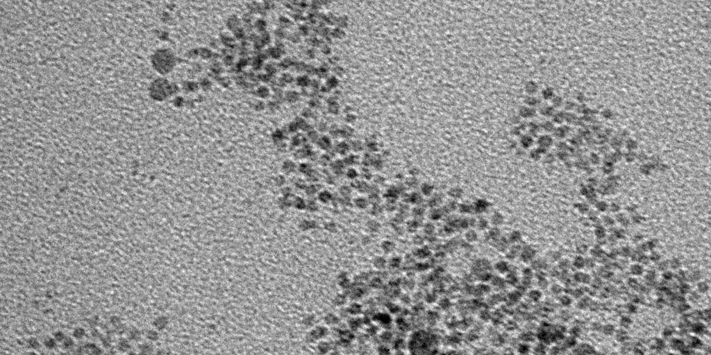
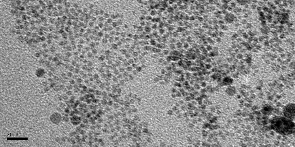
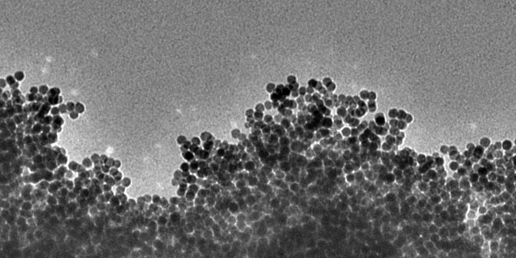
139 122 (a) (b) (c) Figure 4.2: TEM images of magnetite nanoparticles. (a) 4 nm magnetite (b) 9 nm magnetite (c) 16 nm magnetite (Agarwal, 2007).