STUDENT TEXTBOOK JUST-IN-TIME MATH SKILLS SUPPORT FOR MATH 135P MATH FOR LIBERAL ARTS PLUS

Transcription

1 STUDENT TEXTBOOK JUST-IN-TIME MATH SKILLS SUPPORT FOR MATH 135P MATH FOR LIBERAL ARTS PLUS Page 1

2 Beginning and Intermediate Algebra An open source (CC-BY) textbook Available for free download at: by Tyler Wallace Page 2

3 ISBN # Copyright 2010, Some Rights Reserved CC-BY. Beginning and Intermediate Algebra by Tyler Wallace is licensed under a Creative Commons Attribution 3.0 Unported License. ( Based on a work at You are free: to Share: to copy, distribute and transmit the work to Remix: to adapt the work Under the following conditions: Attribution: You must attribute the work in the manner specified by the author or licensor (but not in any way that suggests that they endorse you or your use of the work). With the understanding that: Waiver: Any of the above conditions can be waived if you get permission from the copyright holder. Public Domain: Where the work or any of its elements is in the public domain under applicable law, that status is in no way affected by the license. Other Rights: In no way are any of the following rights affected by the license: Your fair dealing or fair use rights, or other applicable copyright exceptions and limitations; The author s moral rights; Rights other persons may have either in the work itself or in how the work is used such as publicity or privacy rights Notice: For any reuse or distribution, you must make clear to others the license term of this work. The best way to do this is with a link to the following web page: This is a human readable summary of the full legal code which can be read at the following URL: Page 3

4 Special thanks to: My beautiful wife, Nicole Wallace who spent countless hours typing problems and my two wonderful kids for their patience and support during this project Another thanks goes to the faculty reviewers who reviewed this text: Donna Brown, Michelle Sherwood, Ron Wallace, and Barbara Whitney One last thanks to the student reviewers of the text: Eloisa Butler, Norma Cabanas, Irene Chavez, Anna Dahlke, Kelly Diguilio, Camden Eckhart, Brad Evers, Lisa Garza, Nickie Hampshire, Melissa Hanson, Adriana Hernandez, Tiffany Isaacson, Maria Martinez, Brandon Platt, Tim Ries, Lorissa Smith, Nadine Svopa, Cayleen Trautman, and Erin White Page 4

5 Acknowledgments for the notes on Graphing Linear Inequalities and Systems of Linear Inequalities From Chapters 2 and 3 of Elementary Algebra by John Redden. This is an open source textbook. Available for free download at: About the Author John Redden earned his degrees at California State University Northridge and Glendale Community College. He is now a professor of mathematics at the College of the Sequoias, located in Visalia, California. With over a decade of experience working with students to develop their algebra skills, he knows just where they struggle and how to present complex techniques in more understandable ways. His student-friendly and commonsense approach carries over to his writing of Intermediate Algebra and various other open-source learning resources. I would like to thank the following reviewers whose feedback helped improve the final product: Katherine Adams, Eastern Michigan University Sheri Berger, Los Angeles Valley College Seung Choi, Northern Virginia Community College Stephen DeLong, Colorado Mountain College Keith Eddy, College of the Sequoias Solomon Emeghara, William Patterson University Audrey Gillant, SUNY Maritime Barbara Goldner, North Seattle Community College Joseph Grich, William Patterson University Caroll Hobbs, Pensacola State College Clark Ingham, Mott Community College Valerie LaVoice, NHTI, Concord Community College Sandra Martin, Brevard Schools Bethany Mueller, Pensacola State College Tracy Redden, College of the Sequoias James Riley, Northern Arizona University Bamdad Samii, California State University Northridge Michael Scott, California State University Monterey Bay Nora Wheeler, Santa Rosa Junior College I would also like to acknowledge Michael Boezi and Vanessa Gennarelli of Unnamed Publisher. The success of this project is in large part due to their vision and expertise. Finally, a special heartfelt thank-you is due to my wife, Tracy, who spent countless hours proofreading and editing these pages all this while maintaining a tight schedule for our family. Without her, this textbook would not have been possible. Page 5

6 Table of Contents I. Just-In-Time Math Skills Support for Voting Theory and Identification Numbers A. Pre-Algebra Integers Practice Problems Integers Fractions Practice Problems Fractions II. Just-In-Time Math Skills Support for Finance and Fair Division 23 A. Pre-Algebra Order of Operations Practice Problems Order of Operations Properties of Algebra Practice Problems Properties of Algebra B. Solving Linear Equations One Step Equations Practice Problems One Step Equations Two Step Equations Practice Problems Two Step Equations General Equations Practice Problems General Equations Fractions Practice Problems Fractions Formulas Practice Problems Formulas Word Problems: Number and Geometry Practice Problems Word Problems: Number and Geometry Problems Page 6

7 C. Polynomials Exponents Properties Practice Problems Exponents Properties Negative Exponents Practice Problems Negative Exponents Scientific Notation Practice Problems - Scientific Notation Introduction to Polynomials Practice Problems Introduction to Polynomials Multiplying Polynomials Practice Problems Multiplying Polynomials Multiplying Special Products Practice Problems Multiplying Special Products Divide Polynomials Practice Problems Divide Polynomials III. Just-In-Time Math Skills Support for Linear Programming and Statistics. 105 A. Graphing Lines Points and Lines Practice Problems Points and Lines Slope Practice Problems Slope Slope and Intercept Form Practice Problems Slope and Intercept Form Point-Slope Form Practice Problems Point-Slope Form B. Systems of Linear Equations Graphing Practice Problems Graphing Substitution Practice Problems Substitution Addition/Elimination Page 7

8 6. Practice Problems Elimination C. Graphing Linear Inequalities Identify and check solutions Practice Problems Identify and check solutions Graphing Practice Problems Graphing. 155 D. Systems of Linear Inequalities Check Solutions Practice Problems Check Solutions Graph Solutions Practice Problems Graph Solutions 165 IV. Appendix: Answers to All Practice Problems Just-In-Time Math Skills Support for Voting Theory and Identification Numbers. 167 A. Pre-Algebra Answers to Practice Problems Integers Answers to Practice Problems Fractions Just-In-Time Math Skills Support for Finance and Fair Division A. Pre-Algebra Answers to Practice Problems Order of Operations Answers to Practice Problems Properties of Algebra B. Solving Linear Equations Answers to Practice Problems One Step Equations Answers to Practice Problems Two Step Equations Answers to Practice Problems General Equations Answers to Practice Problems Fractions Answers to Practice Problems Formulas Answers to Practice Problems Word Problems. 176 Page 8

9 C. Polynomials Answers to Practice Problems Exponents Properties Answers to Practice Problems Negative Exponents Answers to Practice Problems Scientific Notation Answers to Practice Problems Introduction to Polynomials Answers to Practice Problems Multiplying Polynomials Answers to Practice Problems Multiplying Special Products Answers to Practice Problems Divide Polynomials 183 Just-In-Time Math Skills Support for Linear Programming and Statistics. A. Graphing Lines Answers to Practice Problems Points and Lines Answers to Practice Problems Slope Answers to Practice Problems Slope and Intercept Form Answers to Practice Problems Point-Slope Form. 189 B. Systems of Equations Answers to Practice Problems Graphing Answers to Practice Problems Substitution Answers to Practice Problems Elimination. 192 C. Graphing Linear Inequalities Answers to Practice Problems Identify and check solutions Answers to Practice Problems Graphing. 194 D. Systems of Linear Inequalities Answers to Practice Problems Check Solutions Answers to Practice Problems Graph Solutions. 199 Page 9

10 JUST-IN-TIME MATH SKILLS SUPPORT FOR VOTING THEORY AND IDENTIFICATION NUMBERS Page 10

11 Pre-Algebra - Integers Objective: Add, Subtract, Multiply and Divide Positive and Negative Numbers. The ability to work comfortably with negative numbers is essential to success in algebra. For this reason we will do a quick review of adding, subtracting, multiplying and dividing of integers. Definition: Integers are all the positive whole numbers, zero, and their opposites (negatives). As this is intended to be a review of integers, the descriptions and examples will not be as detailed as a normal lesson. World View Note: The first set of rules for working with negative numbers was written out by the Indian mathematician Brahmagupta. Adding Integers When adding integers we have two cases to consider. Case I: The first is if the signs match, both positive or both negative. If the signs match we will add the numbers together and keep the sign. This is illustrated in the following examples Example ( 3) 8 Same sign, add 5 +3, keep the negative Our Solution Example ( 5) 12 Same sign, add 7 +5, keep the negative Our Solution Case II: If the signs don t match, one positive and one negative number, we will subtract the numbers (as if they were all positive) and then use the sign from the larger number. This means if the larger number is positive, the answer is positive. If the larger number is negative, the answer is negative. This is shown in the following examples. Example Different signs, subtract 7 2, use sign from bigger number, negative Our Solution Page 11

12 Example Different signs, subtract 6 4, use sign from bigger number, positive 2 Our Solution Example ( 3) Different signs, subtract 4 3, use sign from bigger number, positive 1 Our Solution Example ( 10) Different signs, subtract 10 7, use sign from bigger number, negative 3 Our Solution Subtracting Integers For subtraction of negatives we will change the problem to an addition problem which we can then solve using the above methods. The way we change a subtraction to an addition is to add the opposite of the number after the subtraction sign. Often this method is refered to as add the opposite. This is illustrated in the following examples. Example Add the opposite of ( 3) Different signs, subtract 8 3, use sign from bigger number, positive 5 Our Solution Example Add the opposite of ( 6) Same sign, add 4 +6, keep the negative 10 Our Solution Example 9. 9 ( 4) Add the opposite of Same sign, add 9 +4, keep the positive 13 Our Solution Page 12

13 Example ( 2) Add the opposite of 2 Different sign, subtract6 2, use sign from bigger number, negative Our Solution Multiplying and Dividing Integers Multiplication and division of integers both work in a very similar pattern. The short description of the process is we multiply and divide like normal, if the signs match (both positive or both negative) the answer is positive. If the signs don t match (one positive and one negative) then the answer is negative. This is shown in the following examples. Example 11. (4)( 6) 24 Signs do not match, answer is negative Our Solution Example Signs match, answer is positive 4 Our Solution Example 13. 2( 6) Signs match, answer is positive 12 Our Solution Example Signs do not match, answer is negative Our Solution Page 13

14 Common Errors With Integers A few things to be careful of when working with integers. 1. First be sure not to confuse a problem like 3 8 with 3( 8). The second problem is a multiplication problem because there is nothing between the 3 and the parenthesis. If there is no operation written in between the parts, then we assume that means we are multiplying. The 3 8 problem, is subtraction because the subtraction separates the 3 from what comes after it. 2. Another item to watch out for is to be careful not to mix up the pattern for adding and subtracting integers with the pattern for multiplying and dividing integers. They can look very similar, for example if the signs match on addition, the we keep the negative, 3 + ( 7) = 10, but if the signs match on multiplication, the answer is positive, ( 3)( 7) = 21. Page 14

15 Practice - Pre-Algebra -Integers Evaluate each expression. 1) 1 3 3) ( 6) ( 8) 5) ( 3) 3 7) 3 ( 5) 9) ( 7) ( 5) 11) 3 ( 1) 13) ) ( 5)+3 17) ) ( 8) ( 5) 21) ( 2)+( 5) 23) 5 ( 6) 25) ( 6)+3 27) ) ( 7)+7 2) 4 ( 1) 4) ( 6)+8 6) ( 8) ( 3) 8) ) ( 4)+( 1) 12) ( 1)+( 6) 14) ( 8)+( 1) 16) ( 1) 8 18) ) ( 5)+7 22) 1 +( 1) 24) 8 ( 1) 26) ( 3)+( 1) 28) ) ( 3)+( 5) Find each product. 31) (4)( 1) 33) (10)( 8) 35) ( 4)( 2) 37) ( 7)(8) 39) (9)( 4) 41) ( 5)(2) 43) ( 5)(4) 32) (7)( 5) 34) ( 7)( 2) 36) ( 6)( 1) 38) (6)( 1) 40) ( 9)( 7) 42) ( 2)( 2) 44) ( 3)( 9) Page 15

16 45) (4)( 6) Find each quotient. 46) ) ) ) ) ) ) ) ) ) ) ) ) ) ) Page 16

17 Pre-Algebra - Fractions Objective: Reduce, add, subtract, multiply, and divide with fractions. Working with fractions is a very important foundation to algebra. Here we will briefly review reducing, multiplying, dividing, adding, and subtracting fractions. As this is a review, concepts will not be explained in detail as other lessons are. World View Note: The earliest known use of fraction comes from the Middle Kingdom of Egypt around 2000 BC! Reducing Fractions We always like our final answers when working with fractions to be reduced. Reducing fractions is simply done by dividing both the numerator and denominator by the same number. This is shown in the following example Example = = 3 7 Both numerator and denominator are divisible by 4 Both numerator and denominator are still divisible by 3 Our Solution The previous example could have been done in one step by dividing both numerator and denominator by 12. We also could have divided by 2 twice and then divided by 3 once (in any order). It is not important which method we use as long as we continue reducing our fraction until it cannot be reduced any further. Multiplying Fractions The easiest operation with fractions is multiplication. We can multiply fractions by multiplying straight across, multiplying numerators together and denominators together. Example Multiply numerators across and denominators across Our Solution Page 17

18 When multiplying we can reduce our fractions before we multiply. We can either reduce vertically with a single fraction, or diagonally with several fractions, as long as we use one number from the numerator and one number from the denominator. Example Reduce 25 and 55 by dividing by 5. Reduce 32 and 24 by dividing by 8 Multiply numerators across and denominators across Our Solution Dividing Fractions Dividing fractions is very similar to multiplying with one extra step. Dividing fractions requires us to first take the reciprocal of the second fraction and multiply. Once we do this, the multiplication problem solves just as the previous problem. Example Multiply by the reciprocal Reduce 21 and 28 by dividing by 7. Reduce 6 and 16 by dividing by 2 Multiply numerators across and denominators across Our Soultion Adding and Subtracting Fractions To add and subtract fractions we will first have to find the least common denominator (LCD). There are several ways to find an LCD. One way is to find the smallest multiple of the largest denominator that you can also divide the small denomiator by. Example 5. Find the LCD of 8 and 12 Test multiples of 12 12? 12 8 Can t divide 12 by 8 24? 24 8 =3 Yes! We can divide 24 by 8! 24 Our Solution Page 18

19 Adding and subtracting fractions is identical in process. If both fractions already have a common denominator we just add or subtract the numerators and keep the denominator. Example Same denominator, add numerators Reduce answer, dividing by 2 Our Solution While 5 can be written as the mixed number 4 11, in algebra we will almost never 4 use mixed numbers. For this reason we will always use the improper fraction, not the mixed number. Example Same denominator, subtract numerators 13 9 Reduce answer, dividing by 2 Our Solution If the denominators do not match we will first have to identify the LCD and build up each fraction by multiplying the numerators and denominators by the same number so the denominator is built up to the LCD. Example LCD is 18. Multiply the numerator and denominator of the first fraction by 3, and multiply the numerator and deonominator of the second fraction by 2 Same denominator, add numerators, Our Solution Page 19

20 Example LCD is 6 Multiply the numerator and denominator of the first fraction by 2, the second fraction already has a denominator of 6 Same denominator, subtract numerators, 4 1 Reduce answer, dividing by 3 Our Solution Page 20

21 Practice - Pre-Algebra -Fractions Simplify each. Leave your answer as an improper fraction. 1) ) ) ) ) ) ) ) ) ) ) ) ) ) ) ) ) ) ) ) Find each product. 21) (9)( 8 9 ) 23) (2)( 2 9 ) 25) ( 2)( 13 8 ) 27) ( 6 5 )( 11 8 ) 29) (8)( 1 2 ) 31) ( 2 3 )(3 4 ) 33 (2)( 3 2 ) 35) ( 1 2 )( 7 5 ) 22) ( 2)( 5 6 ) 24) ( 2)( 1 3 ) 26) ( 3 2 )(1 2 ) 28) ( 3 7 )( 11 8 ) 30) ( 2)( 9 7 ) 32) ( 17 9 )( 3 5 ) 34) ( 17 9 )( 3 5 ) 36) ( 1 2 )(5 7 ) Page 21

22 Find each quotient. 37) ) ) ) ) ) ) ) Evaluate each expression. 53) ( 4 3 ) 55) ) ) ) ) ( 2 7 ) 65) 1 +( 1 3 ) 67) ( 1 2 ) ) ) ( 5 7 ) ) ) ) ( 15 8 ) ) ( 1) ( 1 6 ) 81) 5 3 ( 1 3 ) 38) ) ) ) ) ) ) ) ) ) ( 11 7 ) 58) ( 2)+( 15 8 ) 60) ( 1) ) ) ( 2) ) ) ) ) ( 1 3 )+( 8 5 ) 74) ( 6)+( 5 3 ) 76) ( 1) ( 1 3 ) 78) ) ( 1 2 ) ( 3 5 ) 82) 9 7 ( 5 3 ) Page 22

23 JUST-IN-TIME MATH SKILLS SUPPORT FOR FINANCE AND FAIR DIVISION Page 23

24 Pre-Algebra - Order of Operations Objective: Evaluate expressions using the order of operations, including the use of absolute value. When simplifying expressions it is important that we simplify them in the correct order. Consider the following problem done two different ways: Example Add First Multiply 7 3 Multiply Add 21 Solution 17 Solution The previous example illustrates that if the same problem is done two different ways we will arrive at two different solutions. However, only one method can be correct. It turns out the second method, 17, is the correct method. The order of operations ends with the most basic of operations, addition (or subtraction). Before addition is completed we must do repeated addition or multiplication (or division). Before multiplication is completed we must do repeated multiplication or exponents. When we want to do something out of order and make it come first we will put it in parenthesis (or grouping symbols). This list then is our order of operations we will use to simplify expressions. Order of Operations: Parenthesis (Grouping) Exponents Multiply and Divide (Left to Right) Add and Subtract (Left to Right) Multiply and Divide are on the same level because they are the same operation (division is just multiplying by the reciprocal). This means they must be done left to right, so some problems we will divide first, others we will multiply first. The same is true for adding and subtracting (subtracting is just adding the opposite). Often students use the word PEMDAS to remember the order of operations, as the first letter of each operation creates the word PEMDAS. However, it is the author s suggestion to think about PEMDAS as a vertical word written as: P E MD AS so we don t forget that multiplication and division are done left to right (same with addition and subtraction). Another way students remember the order of operations is to think of a phrase such as Please Excuse My Dear Aunt Sally where each word starts with the same letters as the order of operations start with. Page 24

25 World View Note: The first use of grouping symbols are found in 1646 in the Dutch mathematician, Franciscus van Schooten s text, Vieta. He used a bar over the expression that is to be evaluated first. So problems like 2(3 + 5) were written as Example (9 4) 2 Parenthesis first 2 +3(5) 2 Exponents 2 + 3(25) Multiply Add 77 Our Solution It is very important to remember to multiply and divide from from left to right! Example Divide first (left to right!) 10 2 Multiply 20 Our Solution In the previous example, if we had multiplied first, five would have been the answer which is incorrect. If there are several parenthesis in a problem we will start with the inner most parenthesis and work our way out. Inside each parenthesis we simplify using the order of operations as well. To make it easier to know which parenthesis goes with which parenthesis, different types of parenthesis will be used such as { } and [ ] and ( ), these parenthesis all mean the same thing, they are parenthesis and must be evaluated first. Example 4. 2{8 2 7[32 4(3 2 +1)]( 1)} Inner most parenthesis, exponents first 2{8 2 7[32 4(9 +1)]( 1)} Add inside those parenthesis 2{8 2 7[32 4(10)]( 1)} Multiply inside inner most parenthesis 2{8 2 7[32 40]( 1)} Subtract inside those parenthesis 2{8 2 7[ 8]( 1)} Exponents next 2{64 7[ 8]( 1)} Multiply left to right, sign with the number 2{ ( 1)} Finish multiplying 2{64 56} Subtract inside parenthesis 2{8} Multiply 16 Our Solution Page 25

26 As the above example illustrates, it can take several steps to complete a problem. The key to successfully solve order of operations problems is to take the time to show your work and do one step at a time. This will reduce the chance of making a mistake along the way. There are several types of grouping symbols that can be used besides parenthesis. One type is a fraction bar. If we have a fraction, the entire numerator and the entire denominator must be evaluated before we reduce the fraction. In these cases we can simplify in both the numerator and denominator at the same time. Example ( 8) Exponent in the numerator, divide in denominator 16 ( 8) Multiply in the numerator, subtract in denominator 16 ( 24) Add the opposite to simplify numerator, denominator is done. Reduce, divide 20 Our Solution Another type of grouping symbol that also has an operation with it, absolute value. When we have absolute value we will evaluate everything inside the absolute value, just as if it were a normal parenthesis. Then once the inside is completed we will take the absolute value, or distance from zero, to make the number positive. Example ( 8) ( 5) 2 Evaluate absolute values first, exponents ( 8) Add inside absolute values Evaluate absolute values 1 +3(8)+2(28) Multiply left to right (28) Finish multiplying Add left to right Add 81 Our Solution Page 26

27 The above example also illustrates an important point about exponents. Exponents only are considered to be on the number they are attached to. This means when we see 4 2, only the 4 is squared, giving us (4 2 ) or 16. But when the negative is in parentheses, such as ( 5) 2 the negative is part of the number and is also squared giving us a positive solution, 25. Page 27

28 Practice - Pre-Algebra-Order of Operations Solve. 1) 6 4( 1) 3) 3 + (8) 4 5) ) [ 9 (2 5)] ( 6) 9) 6 +( 3 3) ) ) [ 1 ( 5)] ) ) [ ( 6)]( ) 21) 6 23) 25) ( 1) 3 + ( 6) [ 1 ( 3)] 8 4 +( 4) [ 4 ( 3)] ( ) ( 4) [ 5( 1)( 5)] [5 + 3(2 2 5)] ) 2) ( 6 6) 3 4) 5( 5 +6) 6 2 6) ) ( ) ( 4) 10) ( 7 5) [ 2 2 ( 6)] 12) 10 6 ( 2) ) 3 {3 [ 3(2 + 4) ( 2)]} 16) 4 [2 + 4( 6) ] 18) 2 ( 3)+3 6[ 2 ( 1 3)] 20) 52 + ( 5) ) 9 2 (3 6) 1 ( 2 + 1) ( 3) 24) 13+ ( 3)2 + 4( 3)+1 [ 10 ( 6)] {[4+5] [ (4 3) 8]}+12 Page 28

29 Pre-Algebra - Properties of Algebra Objective: Simplify algebraic expressions by substituting given values, distributing, and combining like terms. In algebra we will often need to simplify an expression to make it easier to use. There are three basic forms of simplifying which we will review here. World View Note: The term Algebra comes from the Arabic word al-jabr which means reunion. It was first used in Iraq in 830 AD by Mohammad ibn- Musa al-khwarizmi. The first form of simplifying expressions is used when we know what number each variable in the expression represents. If we know what they represent we can replace each variable with the equivalent number and simplify what remains using order of operations. Example 1. p(q + 6) when p =3and q = 5 Replace p with 3 and q with 5 (3)((5) + 6) Evaluate parenthesis (3)(11) Multiply 33 Our Solution Whenever a variable is replaced with something, we will put the new number inside a set of parenthesis. Notice the 3 and 5 in the previous example are in parenthesis. This is to preserve operations that are sometimes lost in a simple replacement. Sometimes the parenthesis won t make a difference, but it is a good habbit to always use them to prevent problems later. Example 2. ( ) x x + zx(3 z) when x= 6 and z = 2 Replace allx s with 6 andz s with 2 3 ( ) ( 6) ( 6) +( 2)( 6)(3 ( 2)) Evaluate parenthesis (5)( 2) Multiply left to right (5)( 2) ( 2) Multiply left to right Multiply Subtract Our Solution It will be more common in our study of algebra that we do not know the value of the variables. In this case, we will have to simplify what we can and leave the variables in our final solution. One way we can simplify expressions is to combine like terms. Page 29

30 Definition: Like terms are terms where the variables match exactly (exponents included). Examples of like terms would be 3xy and 7xy or 3a 2 b and 8a 2 b or 3 and 5. If we have like terms we are allowed to add (or subtract) the numbers in front of the variables, then keep the variables the same. This is shown in the following examples. Example 3. 5x 2y 8x +7y 3x + 5y Combine like terms 5x 8x and 2y + 7y Our Solution Example 4. 8x 2 3x +7 2x 2 +4x 3 Combine like terms 8x 2 2x 2 and 3x +4x and 7 3 6x 2 + x +4 Our Solution As we combine like terms we need to interpret subtraction signs as part of the following term. This means if we see a subtraction sign, we treat the following term like a negative term, the sign always stays with the term. A final method to simplify is known as distributing. Often as we work with problems there will be a set of parenthesis that make solving a problem difficult, if not impossible. To get rid of these unwanted parenthesis we have the distributive property. Using this property we multiply the number in front of the parenthesis by each term inside of the parenthesis. Distributive Property: a(b+c)=ab + ac Several examples of using the distributive property are given below. Example 5. 4(2x 7) Multiply each term by 4 8x 28 Our Solution Example 6. 7(5x 6) Multiply each term by 7 Our Solution Page 30

31 In the previous example we again use the fact that the sign goes with the number, this means we treat the 6 as a negative number, this gives ( 7)( 6) = 42, a positive number. The most common error in distributing is a sign error, be very careful with your signs! It is possible to distribute just a negative through parenthesis. If we have a negative in front of parenthesis we can think of it like a 1 in front and distribute the 1 through. This is shown in the following example. Example 7. (4x 5y +6) 1(4x 5y +6) 4x + 5y 6 Negative can be thought of as 1 Multiply each term by 1 Our Solution Distributing through parenthesis and combining like terms can be combined into one problem. Order of operations tells us to multiply (distribute) first then add or subtract last (combine like terms). Thus we do each problem in two steps, distribute then combine. Example (2x 4) Distribute 3, multipling each term 5 + 6x 12 Combine like terms x Our Solution Example 9. 3x 2(4x 5) 3x 8x x + 10 Distribute 2, multilpying each term Combine like terms 3x 8x Our Solution In the previous example we distributed 2, not just 2. This is because we will always treat subtraction like a negative sign that goes with the number after it. This makes a big difference when we multiply by the 5 inside the parenthesis, we now have a positive answer. Following are more involved examples of distributing and combining like terms. Example 10. 2(5x 8) 6(4x +3) Distribute2into first parenthesis and 6 into second 10x 16 24x 18 Combine like terms 10x 24x and x 34 Our Solution Page 31

32 Example 11. 4(3x 8) (2x 7) Negative (subtract) in middle can be thought of as 1 4(3x 8) 1(2x 7) Distribute 4 into first parenthesis, 1 into second 12x 32 2x + 7 Combine like terms 12x 2x and x 25 Our Solution Page 32

33 Practice - Pre-Algebra-Properties of Algebra Evaluate each using the values given. 1) p+1+ q m; use m =1, p =3, q =4 3) p pq ; use p=6and q =5 6 5) c 2 (a 1); use a =3and c=5 7) 5j + kh ; useh=5, j = 4,k =2 2 9) 4 (p m) 2 + q; use m =4, p=6, q = 6 11) m +n+m+ n ; use m = 1 and n =2 2 2) y 2 + y z; use y =5, z =1 4) 6+z y ; use y = 1,z = 4 3 6) x +6z 4y; use x =6, y = 4,z =4 8) 5(b +a)+1+c; use a=2,b=6,c=5 10) z +x (1 2 ) 3 ; use x =5, z =4 12) 3 +z 1 + y 1; use y = 5,z = 4 13) q p (q 1 3); use p=3, q = 6 14) p+(q r)(6 p); use p=6, q = 5,r = 5 15) y [4 y (z x)]; use x =3, y = 1,z = 6 16) 4z (x + x (z z)); use x =3, z =2 17) k 3 2 (j + k) 5; use j =4, k =5 19) zx (z 4+x ); usex=2,z =6 6 18) a 3 (c 2 c); use a =3, c=2 20) 5 + qp+ pq q; use p =6, q = 3 Combine Like Terms. 21) r ) n +n 25) 8v +7v 27) 7x 2x 29) k ) x 10 6x ) m 2m 35) 9n 1 +n+4 22) 4x ) 4b b 26) x+8x 28) 7a ) 8p +5p 32) 1 10n 10 34) 1 r 6 36) 4b + 9b Page 33

34 Distribute. 37) 8(x 4) 39) 8n(n +9) 41) 7k( k + 6) 43) 6(1 +6x) 45) 8m(5 m) 47) 9x(4 x) 49) 9b(b 10) 51) 8n(5 + 10n) Simplify. 53) 9(b + 10)+5b 55) 3x(1 4x) 4x 2 57) 4k 2 8k (8k +1) 59) 1 7(5 + 7p) 61) 10 4(n 5) 63) 4(x +7) +8(x +4) 65) 8(n+6) 8n(n+8) 67) 7(7 + 3v) + 10(3 10v) 69) 2n( 10n +5) 7(6 10n) 71) 5(1 6k) + 10(k 8) 73) (8n 2 3n) (5 + 4n 2 ) 75) (5p 6) +(1 p) 77) (2 4v 2 ) +(3v 2 +2v) 79) (4 2k 2 )+(8 2k 2 ) 81) (x 2 8) +(2x 2 7) 38) 3(8v +9) 40) ( 5 +9a) 42) 10x(1 +2x) 44) 2(n+1) 46) 2p(9p 1) 48) 4(8n 2) 50) 4(1 +7r) 52) 2x(8x 10) 54) 4v 7(1 8v) 56) 8x + 9( 9x +9) 58) 9 10(1 + 9a) 60) 10(x 2) 3 62) 6(5 m)+3m 64) 2r(1 +4r)+8r( r +4) 66) 9(6b +5) 4b(b + 3) 68) 7(4x 6)+2(10x 10) 70) 3(4 +a)+6a(9a + 10) 72) 7(4x+3) 10(10x + 10) 74) (7x 2 3) (5x 2 + 6x) 76) (3x 2 x) (7 8x) 78) (2b 8)+(b 7b 2 ) 80) (7a 2 +7a) (6a 2 + 4a) 82) (3 7n 2 )+(6n 2 + 3) Page 34

35 Solving Linear Equations - One Step Equations Objective: Solve one step linear equations by balancing using inverse operations. Solving linear equations is an important and fundamental skill in algebra. In algebra, we are often presented with a problem where the answer is known, but part of the problem is missing. The missing part of the problem is what we seek to find. An example of such a problem is shown below. Example 1. 4x + 16 = 4 Notice the above problem has a missing part, or unknown, that is marked by x. If we are given that the solution to this equation is 5, it could be plugged into the equation, replacing the x with 5. This is shown in Example 2. Example 2. 4( 5) + 16 = 4 Multiply 4( 5) = 4 Add = 4 True! Now the equation comes out to a true statement! Notice also that if another number, for example, 3, was plugged in, we would not get a true statement as seen in Example 3. Example 3. 4(3) + 16 = 4 Multiply 4(3) = 4 Add =/ 4 False! Due to the fact that this is not a true statement, this demonstates that 3 is not the solution. However, depending on the complexity of the problem, this guess and check method is not very efficient. Thus, we take a more algebraic approach to solving equations. Here we will focus on what are called one-step equations or equations that only require one step to solve. While these equations often seem very fundamental, it is important to master the pattern for solving these problems so we can solve more complex problems. Page 35

36 Addition Problems To solve equations, the general rule is to do the opposite. For example, consider the following example. Example 4. x +7= x = 12 The7is added to the x Subtract 7 from both sides to get rid of it Our solution! Then we get our solution, x = 12. The same process is used in each of the following examples. Example x =8 4 4 x = 4 7 = x = x Table 1. Addition Examples 5 = 8 +x =x Subtraction Problems In a subtraction problem, we get rid of negative numbers by adding them to both sides of the equation. For example, consider the following example. Example 6. x 5 =4 The 5 is negative, or subtracted fromx Add 5 to both sides x =9 Our Solution! Then we get our solution x = 9. The same process is used in each of the following examples. Notice that each time we are getting rid of a negative number by adding. Example x = x = 4 10 = x = x Table 2. Subtraction Examples 5 = 8 + x =x Page 36

37 Multiplication Problems With a multiplication problem, we get rid of the number by dividing on both sides. For example consider the following example. Example 8. 4x = 20 Variable is multiplied by Divide both sides by 4 x = 5 Then we get our solution x = 5 Our solution! With multiplication problems it is very important that care is taken with signs. If x is multiplied by a negative then we will divide by a negative. This is shown in example 9. Example 9. 5x = x = 6 Variable is multiplied by 5 Divide both sides by 5 Our Solution! The same process is used in each of the following examples. Notice how negative and positive numbers are handled as each problem is solved. Example 10. 8x = x = 3 4x = x =5 Table 3. Multiplication Examples 42 =7x =x Division Problems In division problems, we get rid of the denominator by multiplying on both sides. For example consider our next example. Example 11. x = 3 Variable is divided by 5 5 (5) x = 3(5) Multiply both sides by5 5 x = 15 Our Solution! Page 37

38 Then we get our solution x = 15. The same process is used in each of the following examples. Example 12. (-7) x 7 = 2 x 7 = 2(-7) x = 14 x 8 = 5 (8) x 8 =5(8) x = 40 Table 4. Division Examples x 4 =9 ( 4) x 4 = 9(-4) x = 36 The process described above is fundamental to solving equations. once this process is mastered, the problems we will see have several more steps. These problems may seem more complex, but the process and patterns used will remain the same. World View Note: The study of algebra originally was called the Cossic Art from the Latin, the study of things (which we now call variables). Page 38

39 Solve each equation. Practice Linear Equations - One Step Equations 1) v + 9 = 16 3)x 11 = 16 5) 30=a+20 7) x 7= 26 9) 13=n 5 11) 340= 17x 13) 9= n 12 15) 20v = ) 340=20n 19) 16x=320 21) 16+n= 13 23) p 8= 21 25) 180=12x 27) 20b= ) r 14 = ) 7=a+4 33) 10=x 4 35) 13a= ) p 20 = 12 39) 9 + m = 7 2) 14=b+3 4) 14 =x 18 6) 1 + k = 5 8) 13 + p = 19 10) 22=16+m 12) 4r= 28 14) 5 = b ) 20x= 80 18) 1 = a ) k = ) 21=x+5 24) m 4= 13 26) 3n=24 28) 17= x 12 30) n+8=10 32) v 16= 30 34) 15=x 16 36) 8k=120 38) 15= x 9 40) 19= n 20 Page 39

40 Linear Equations - Two-Step Equations Objective: Solve two-step equations by balancing and using inverse opperations. After mastering the technique for solving equations that are simple one-step equations, we are ready to consider two-step equations. As we solve two-step equations, the important thing to remember is that everything works backwards! When working with one-step equations, we learned that in order to clear a plus five in the equation, we would subtract five from both sides. We learned that to clear divided by seven we multiply by seven on both sides. The same pattern applies to the order of operations. When solving for our variable x, we use order of operations backwards as well. This means we will add or subtract first, then multiply or divide second (then exponents, and finally any parentheses or grouping symbols, but that s another lesson). So to solve the equation in the first example, Example 1. 4x 20 = 8 We have two numbers on the same side as the x. We need to move the 4 and the 20 to the other side. We know to move the four we need to divide, and to move the twenty we will add twenty to both sides. If order of operations is done backwards, we will add or subtract first. Therefore we will add 20 to both sides first. Once we are done with that, we will divide both sides by 4. The steps are shown below. 4x 20 = 8 Start by focusing on the subtract Add 20 to both sides 4x =12 Now we focus on the 4 multiplied by x 4 4 Divide both sides by 4 x =3 Our Solution! Notice in our next example when we replace the x with 3 statement. we get a true 4(3) 20 = 8 Multiply 4(3) = 8 Subtract = 8 True! The same process is used to solve any two-step equation. Add or subtract first, then multiply or divide. Consider our next example and notice how the same process is applied. Page 40

41 Example 2. 5x +7= 7 Start by focusing on the plus Subtract 7 from both sides 5x = 0 Now focus on the multiplication by Divide both sides by 5 x = 0 Our Solution! Notice the seven subtracted out completely! Many students get stuck on this point, do not forget that we have a number for nothing left and that number is zero. With this in mind the process is almost identical to our first example. A common error students make with two-step equations is with negative signs. Remember the sign always stays with the number. Consider the following example. Example x = 10 Start by focusing on the positive Subtract 4 from both sides 2x =6 2 2 x = 3 Negative(subtraction) stays on the 2x Divide by 2 Our Solution! The same is true even if there is no coefficient in front of the variable. Consider the next example. Example 4. 8 x=2 Start by focusing on the positive Subtract 8 from both sides x = 6 Negative(subtraction) stays on the x 1x = 6 Remember, no number in front of variable means Divide both sides by 1 x =6 Our Solution! Solving two-step equations is a very important skill to master, as we study algebra. The first step is to add or subtract, the second is to multiply or divide. This pattern is seen in each of the following examples. Page 41

42 Example 5. 3x +7= x = x =5 2 +9x = x = x = 1 8 = 2x =2x = x 7 5x = x = x = 2 5 3x = x = x = 0 Table 1. Two-Step Equation Examples 3 = x (5)(1) = x 5 (5) 5 =x As problems in algebra become more complex the process covered here will remain the same. In fact, as we solve problems like those in the next example, each one of them will have several steps to solve, but the last two steps are a twostep equation like we are solving here. This is why it is very important to master two-step equations now! Example 6. 3x x+6 1 x x = 1 3 5x 5 +1=x log 5 (2x 4) =1 World View Note: Persian mathematician Omar Khayyam would solve algebraic problems geometrically by intersecting graphs rather than solving them algebraically. Page 42

43 Solve each equation. Practice Linear Equations - Two-Step Problems 1) 5+ n =4 4 3) 102= 7r +4 5) 8n+3 = 77 7) 0= 6v 9) 8= x ) 0 = 7+ k 2 13) 12+3x=0 15) 24=2n 8 17) 2= 12+2r 19) b +7= ) 152=8n+64 23) 16=8a+64 25) 56+8k =64 27) 2x+4=22 29) 20=4p+4 31) 5=3+ n 2 33) r 6= ) 40=4n 32 37) 87=3 7v 39) x+1= 11 2) 2= 2m+12 4) 27=21 3x 6) 4 b=8 8) 2+ x = ) 5= a ) 6=15+3p 14) 5m+2 = 27 16) 37=8+3x 18) 8+ n = ) x 8= ) 11= 8+ v 2 24) 2x 3= 29 26) 4 3n= 16 28) 67=5m 8 30) 9=8+ x 6 32) m 1= ) 80=4x 28 36) 33=3b+3 38) 3x 3= 3 40) 4+ a =1 3 Page 43

44 Solving Linear Equations - General Equations Objective: Solve general linear equations with variables on both sides. Often as we are solving linear equations we will need to do some work to set them up into a form we are familiar with solving. This section will focus on manipulating an equation we are asked to solve in such a way that we can use our pattern for solving two-step equations to ultimately arrive at the solution. One such issue that needs to be addressed is parenthesis. Often the parenthesis can get in the way of solving an otherwise easy problem. As you might expect we can get rid of the unwanted parenthesis by using the distributive property. This is shown in the following example. Notice the first step is distributing, then it is solved like any other two-step equation. Example 1. 4(2x 6) = 16 Distribute 4 through parenthesis 8x 24 = 16 Focus on the subtraction first Add 24 to both sides 8x = 40 Now focus on the multiply by Divide both sides by 8 x =5 Our Solution! Often after we distribute there will be some like terms on one side of the equation. Example 2 shows distributing to clear the parenthesis and then combining like terms next. Notice we only combine like terms on the same side of the equation. Once we have done this, our next example solves just like any other two-step equation. Example 2. 3(2x 4) +9=15 Distribute the 3 through the parenthesis 6x 12 +9=15 Combine like terms, x 3 = 15 Focus on the subtraction first Add3to both sides 6x = 18 Now focus on multiply by Divide both sides by 6 x =3 Our Solution A second type of problem that becomes a two-step equation after a bit of work is one where we see the variable on both sides. This is shown in the following example. Page 44

45 Example 3. 4x 6 =2x + 10 Notice here the x is on both the left and right sides of the equation. This can make it difficult to decide which side to work with. We fix this by moving one of the terms with x to the other side, much like we moved a constant term. It doesn t matter which term gets moved, 4x or 2x, however, it would be the author s suggestion to move the smaller term (to avoid negative coefficients). For this reason we begin this problem by clearing the positive 2x by subtracting 2x from both sides. 4x 6 = 2x + 10 Notice the variable on both sides 2x 2x Subtract 2x from both sides 2x 6 = 10 Focus on the subtraction first Add 6 to both sides 2x = 16 Focus on the multiplication by Divide both sides by 2 x =8 Our Solution! The next example shows the check on this solution. Here the solution is plugged into the x on both the left and right sides before simplifying. Example 4. 4(8) 6 =2(8) + 10 Multiply 4(8) and 2(8) first 32 6 = Add and Subtract 26 = 26 True! The next example illustrates the same process with negative coefficients. Notice first the smaller term with the variable is moved to the other side, this time by adding because the coefficient is negative. Example 5. 3x + 9 =6x 27 Notice the variable on both sides, 3x is smaller +3x +3x Add 3x to both sides 9 =9x 27 Focus on the subtraction by Add 27 to both sides 36 = 9x Focus on the mutiplication by Divide both sides by 9 4 = x Our Solution Page 45

46 Linear equations can become particularly intersting when the two processes are combined. In the following problems we have parenthesis and the variable on both sides. Notice in each of the following examples we distribute, then combine like terms, then move the variable to one side of the equation. Example 6. 2(x 5)+3x =x+18 Distribute the 2 through parenthesis 2x x =x+18 Combine like terms 2x+3x 5x 10 =x+18 Notice the variable is on both sides x x Subtract x from both sides 4x 10 = 18 Focus on the subtraction of Add 10 to both sides 4x = 28 Focus on multiplication by Divide both sides by 4 x = 7 Our Solution Sometimes we may have to distribute more than once to clear several parenthesis. Remember to combine like terms after you distribute! Example 7. 3(4x 5) 4(2x +1) =5 Distribute 3 and 4 through parenthesis 12x 15 8x 4 =5 Combine like terms 12x 8x and x 19 =5 Focus on subtraction of Add 19 to both sides 4x = 24 Focus on multiplication by Divide both sides by 4 x =6 Our Solution This leads to a 5-step process to solve any linear equation. While all five steps aren t always needed, this can serve as a guide to solving equations. 1. Distribute through any parentheses. 2. Combine like terms on each side of the equation. 3. Get the variables on one side by adding or subtracting 4. Solve the remaining 2-step equation (add or subtract then multiply or divide) Page 46

47 5. Check your answer by plugging it back in for x to find a true statement. The order of these steps is very important. World View Note: The Chinese developed a method for solving equations that involved finding each digit one at a time about 2000 years ago! We can see each of the above five steps worked through our next example. Example 8. 4(2x 6) +9=3(x 7)+8x Distribute 4 and 3 through parenthesis 8x 24 +9=3x x Combine like terms 24 +9and3x + 8x 8x 15 = 11x 21 Notice the variable is on both sides 8x 8x Subtract 8x from both sides 15 = 3x 21 Focus on subtraction of Add 21 to both sides 6 =3x Focus on multiplication by Divide both sides by 3 2 =x Our Solution Check: 4[2(2) 6] +9=3[(2) 7]+8(2) Plug 2 in for each x. Multiply inside parenthesis 4[4 6]+9=3[ 5] +8(2) Finish parentesis on left, multiply on right 4[ 2]+9= 15 +8(2) Finish multiplication on both sides = Add 1 =1 True! When we checked our solution of x = 2 we found a true statement, 1 = 1. Therefore, we know our solution x =2 is the correct solution for the problem. There are two special cases that can come up as we are solving these linear equations. The first is illustrated in the next two examples. Notice we start by distributing and moving the variables all to the same side. Example 9. 3(2x 5)=6x 15 Distribute3through parenthesis 6x 15 =6x 15 Notice the variable on both sides 6x 6x Subtract 6x from both sides 15 = 15 Variable is gone! True! Page 47

48 Here the variable subtracted out completely! We are left with a true statement, 15 = 15. If the variables subtract out completely and we are left with a true statement, this indicates that the equation is always true, no matter what x is. Thus, for our solution we say all real numbers or R. Example 10. 2(3x 5) 4x =2x + 7 Distribute 2 through parenthesis 6x 10 4x =2x + 7 Combine like terms 6x 4x 2x 10 =2x + 7 Notice the variable is on both sides 2x 2x Subtract 2x from both sides 10 =/ 7 Variable is gone! False! Again, the variable subtracted out completely! However, this time we are left with a false statement, this indicates that the equation is never true, no matter what x is. Thus, for our solution we say no solution or. Page 48

49 Practice - Linear Equations - General Linear Equations Solve each equation. 1) 2 ( 3a 8)=1 3) 5( 4 +2v)= 50 5) 66=6(6 + 5x) 7) 0= 8(p 5) 9) 2 +2(8x 7) = 16 11) 21x+12= 6 3x 13) 1 7m= 8m +7 15) 1 12r = 29 8r 17) 20 7b= 12b+30 19) 32 24v=34 2v 21) 2 5(2 4m)=33+5m 23) 4n+ 11=2(1 8n) +3n 25) 6v 29= 4v 5(v+1) 27) 2(4x 4)= 20 4x 29) a 5(8a 1)=39 7a 31) 57= ( p + 1)+2(6+8p) 33) 2(m 2)+7(m 8) = 67 35) 50=8 (7 +7r) (4r +6) 37) 8(n 7) +3(3n 3)=41 39) 61= 5(5r 4)+4(3r 4) 41) 2(8n 4) =8(1 n) 43) 3( 7v+3)+8v=5v 4(1 6v) 45) 7(x 2)= 4 6(x 1) 47) 6(8k + 4)= 8(6k +3) 2 49) 2(1 7p)=8(p 7) 2) 2( 3n+8)= 20 4) 2 8( 4 +3x)=34 6) 32=2 5( 4n + 6) 8) 55=8 + 7(k 5) 10) (3 5n) = 12 12) 3n 27= 27 3n 14) 56p 48=6p+2 16) 4 +3x= 12x+4 18) 16n+12=39 7n 20) 17 2x=35 8x 22) 25 7x=6(2x 1) 24) 7(1+b) = 5 5b 26) 8(8r 2)=3r+16 28) 8n 19= 2(8n 3) +3n 30) 4+4k =4(8k 8) 32) 16= 5(1 6x)+3(6x +7) 34) 7=4(n 7)+5(7n+7) 36) 8(6+6x)+4( 3 +6x)= 12 38) 76=5(1 + 3b) +3(3b 3) 40) 6(x 8) 4(x 2) = 4 42) 4(1 +a)=2a 8(5+3a) 44) 6(x 3)+5= 2 5(x 5) 46) (n+8)+n = 8n + 2(4n 4) 48) 5(x+7)=4( 8x 2) 50) 8( 8n+4)=4( 7n+8) Page 49

50 Solving Linear Equations - Fractions Objective: Solve linear equations with rational coefficients by multiplying by the least common denominator to clear the fractions. Often when solving linear equations we will need to work with an equation with fraction coefficients. We can solve these problems as we have in the past. This is demonstrated in our next example. Example x 7 2 = Focus on subtraction Add 7 to both sides 2 Notice we will need to get a common denominator to add Notice we have a 6 2 common denominator of 6. So we build up the denominator, 7 ( 3 ) =, and we 6 can now add the fractions: 3 4 x 21 6 = 5 6 Same problem, with common denominator Add 21 6 to both sides 3 4 x = 26 6 Reduce 26 6 to x = 13 3 Focus on multiplication by 3 4 We can get rid of 3 by dividing both sides by 3. Dividing by a fraction is the 4 4 same as multiplying by the reciprocal, so we will multiply both sides by 4. 3 ( ) x = 13 3 x = 52 9 ( ) 4 3 Multiply by reciprocal Our solution! While this process does help us arrive at the correct solution, the fractions can make the process quite difficult. This is why we have an alternate method for dealing with fractions - clearing fractions. Clearing fractions is nice as it gets rid of the fractions for the majority of the problem. We can easily clear the fractions by finding the LCD and multiplying each term by the LCD. This is shown in the Page 50

51 next example, the same problem as our first example, but this time we will solve by clearing fractions. Example x 7 2 = 5 6 (12)3 x (12)7 = (12) LCD =12, multiply each term by 12 Reduce each 12 with denominators (3)3x (6)7 =(2)5 Multiply out each term 9x 42 = 10 Focus on subtraction by Add 42 to both sides 9x = 52 Focus on multiplication by Divide both sides by 9 x = 52 9 Our Solution The next example illustrates this as well. Notice the 2 isn t a fraction in the original equation, but to solve it we put the 2 over 1 to make it a fraction. Example x 2 = 3 2 x (6)2 3 x (6)2 = (6)3 1 2 x + (6)1 6 LCD =6, multiply each term by 6 Reduce 6 with each denominator (2)2x (6)2 =(3)3x +(1)1 Multiply out each term 4x 12 = 9x +1 Notice variable on both sides 4x 4x Subtract 4x from both sides 12 = 5x +1 Focus on addition of1 1 1 Subtract 1 from both sides 13 =5x Focus on multiplication of5 5 5 Divide both sides by =x Our Solution We can use this same process if there are parenthesis in the problem. We will first distribute the coefficient in front of the parenthesis, then clear the fractions. This is seen in the following example. Page 51

52 Example 4. ( x (18)5 x + (18) (3)5x +(2)2 =(18)3 ) = 3 Distribute 3 through parenthesis, reducing if possible x + 2 = 3 9 LCD =18, multiply each term by 18 = (18)3 Reduce 18 with each denominator 15x +4= Multiply out each term Focus on addition of4 Subtract 4 from both sides 15x = 50 Focus on multiplication by Divide both sides by 15. Reduce on right side. x = 10 Our Solution 3 While the problem can take many different forms, the pattern to clear the fraction is the same, after distributing through any parentheses we multiply each term by the LCD and reduce. This will give us a problem with no fractions that is much easier to solve. The following example again illustrates this process. Example x 1 2 = 1 3 (3 4 x + 6) x 1 2 = 1 4 x (4)3 4 x (4)1 = (4)1 2 4 x + (4)2 (4)7 1 2 Distribute 1, reduce if possible 3 LCD =4, multiply each term by 4. Reduce 4 with each denominator (1)3x (2)1 =(1)1x +(4)2 (2)7 Multiply out each term 3x 2 =x+8 14 Combine like terms x 2 =x 6 Notice variable on both sides x x Subtract x from both sides 2x 2 = 6 Focus on subtraction by Add2to both sides 2x = 4 Focus on multiplication by Divide both sides by 2 x = 2 Our Solution World View Note: The Egyptians were among the first to study fractions and linear equations. The most famous mathematical document from Ancient Egypt is the Rhind Papyrus where the unknown variable was called heap Page 52

53 Practice - Linear Equations-Fractions Solve each equation. 1) 3 21 (1 + p)= ) 0 = 5 4 (x 6 5 ) 5) m = ) = 5 2 ( x) 9) 2b = ) 3 2 (7 3 n+1)= ) a 5 4 ( 8 3 a +1) = ) 55 6 = 5 2 (3 2 p 5 3 ) 17) 16 9 = 4 3 ( 4 3 n 4 3 ) 19) 5 8 = 5 4 (r 3 2 ) 21) b= 5 2 (b 5 3 ) 23) ( 5 2 x 3 2 ) = 3 2 +x 25) n= 7 n ) 3 2 (v ) = 7 4 v ) x = 5 3 (5 2 x +1) 2) 1 2 = 3 2 k ) 3 2 n 8 3 = ) r = ) 16 9 = 4 3 (5 3 + n) 10) v = ) 41 9 = 5 2 (x ) 1 3 x 14) 1 3 ( 7 4 k +1) 10 3 k = ) 1 2 (2 3 x 3 4 ) 7 2 x = ) 2 (m + 9 ) 10 = ) 1 12 = 4 3 x (x 7 4 ) 22) n = 3 2 n + 2(n+ 3 2 ) 24) r= 7 4 r 5 4 ( 4 3 r + 1) 26) 7 2 (5 3 a )= 11 4 a ) 8 1 x = 3 2 4x 2 13 ( x+1) ) 1 3 n = 2(4 3 n ) Page 53

54 Solving Linear Equations - Formulas Objective: Solve linear formulas for a given variable. Solving formulas is much like solving general linear equations. The only difference is we will have several varaibles in the problem and we will be attempting to solve for one specific variable. For example, we may have a formula such as A = πr 2 + πrs (formula for surface area of a right circular cone) and we may be interested in solving for the varaible s. This means we want to isolate the s so the equation has s on one side, and everything else on the other. So a solution might look like s = A πr2. This second equation gives the same information as the first, πs they are algebraically equivalent, however, one is solved for the area, while the other is solved for s (slant height of the cone). In this section we will discuss how we can move from the first equation to the second. When solving formulas for a variable we need to focus on the one varaible we are trying to solve for, all the others are treated just like numbers. This is shown in the following example. Two parallel problems are shown, the first is a normal onestep equation, the second is a formula that we are solving for x. Example 1. 3x = 12 wx =z In both problems, x is multiplied by something 3 3 w w To isolate the x we divide by 3 or w. x = 4 x = z Our Solution w We use the same process to solve 3x = 12 for x as we use to solve wx = z for x. Because we are solving for x we treat all the other variables the same way we would treat numbers. Thus, to get rid of the multiplication we divided by w. This same idea is seen in the following example. Example 2. m +n= p forn Solving for n, treat all other variables like numbers m m Subtract m from both sides n = p m Our Solution As p and m are not like terms, they cannot be combined. For this reason we leave the expression as p m. This same one-step process can be used with grouping symbols. Page 54

55 Example 3. a(x y) = b fora Solving for a, treat(x y) like a number (x y) (x y) Divide both sides by (x y) a= b x y Our Solution Because (x y) is in parenthesis, if we are not searching for what is inside the parenthesis, we can keep them together as a group and divide by that group. However, if we are searching for what is inside the parenthesis, we will have to break up the parenthesis by distributing. The following example is the same formula, but this time we will solve for x. Example 4. a(x y)=b for x Solving for x, we need to distribute to clear parenthesis ax ay =b +ay+ay ax =b+ay This isatwo step equation, ay is subtracted from our x term Add ay to both sides Thexis multipied by a a a Divide both sides by a x = b + ay Our Solution a Be very careful as we isolate x that we do not try and cancel the a on top and bottom of the fraction. This is not allowed if there is any adding or subtracting in the fraction. There is no reducing possible in this problem, so our final reduced answer remains x = b + ay. The next example is another two-step problem a Example 5. y = mx +b form Solving form, focus on addition first b b Subtract b from both sides y b=mx m is multipied by x. x x Divide both sides by x y b =m Our Solution x It is important to note that we know we are done with the problem when the variable we are solving for is isolated or alone on one side of the equation and it does not appear anywhere on the other side of the equation. The next example is also a two-step equation, it is the problem we started with at the beginning of the lesson. Page 55

56 Example 6. A =πr 2 + πrs fors Solving for s, focus on what is added to the term with s πr 2 πr 2 A πr 2 = πrs Subtract πr 2 from both sides s is multipied by πr πr πr Divide both sides by πr A πr 2 = s Our Solution πr Again, we cannot reduce the πr in the numerator and denominator because of the subtraction in the problem. Formulas often have fractions in them and can be solved in much the same way we solved with fractions before. First identify the LCD and then multiply each term by the LCD. After we reduce there will be no more fractions in the problem so we can solve like any general equation from there. Example 7. h = 2m n (n)h= (n)2m n for m To clear the fraction we use LCD =n Multiply each term by n nh = 2m Reduce n with denominators 2 2 Divide both sides by 2 nh = m Our Solution 2 The same pattern can be seen when we have several fractions in our problem. Example 8. (b)a b a b + c =e fora To clear the fraction we use LCD =b b + (b)c = e(b) Multiply each term by b b a+c=eb Reducebwith denominators c c a =eb c Subtract c from both sides Our Solution Depending on the context of the problem we may find a formula that uses the same letter, one capital, one lowercase. These represent different values and we must be careful not to combine a capital variable with a lower case variable. Page 56

57 Example 9. (2 b)a = a = A 2 b (2 b)a 2 b forb Use LCD (2 b) as a group Multiply each term by (2 b) (2 b)a =A reduce (2 b) with denominator 2a ab = A Distribute through parenthesis 2a 2a Subtract 2a from both sides ab=a 2a The b is multipied by a a a Divide both sides by a b = A 2a Our Solution a Notice the A and a were not combined as like terms. This is because a formula will often use a capital letter and lower case letter to represent different variables. Often with formulas there is more than one way to solve for a variable. The next example solves the same problem in a slightly different manner. After clearing the denominator, we divide by a to move it to the other side, rather than distributing. Example 10. a = A 2 b forb Use LCD =(2 b) asagroup (2 b)a (2 b)a = 2 b Multiply each term by (2 b) (2 b)a =A Reduce (2 b) with denominator a a Divide both sides by a 2 b= A Focus on the positive 2 a 2 2 Subtract 2 from both sides b = A a 2 Still need to clear the negative ( b)= A a 2 Multiply (or divide) each term by 1 b = A a + 2 Our Solution Both answers to the last two examples are correct, they are just written in a different form because we solved them in different ways. This is very common with formulas, there may be more than one way to solve for a varaible, yet both are equivalent and correct. Page 57

58 World View Note: The father of algebra, Persian mathematician Muhammad ibn Musa Khwarizmi, introduced the fundamental idea of blancing by subtracting the same term to the other side of the equation. He called this process al-jabr which later became the world algebra. Page 58

59 Practice - Linear Equations Formulas Solve each of the following equations for the indicated variable. 1) ab = c for b 3) f x =b for x g 5) 3x= a b forx 7) E = mc 2 for m 9) V = 4 3 πr3 for π 11) a + c = b for c 13) c = 4y m+n for y 15) V = πdn 12 for D 17) P =n(p c) for n 19) T = D d L for D 21) L = L o (1+at) forl o 23) 2m + p = 4m + q for m 25) k m r = q for k 27) h= vt 16t 2 for v 29) Q 1 =P(Q 2 Q 1 ) for Q 2 31) R= ka(t 1 + T 2 ) d 33) ax + b = c for a 35) lwh = V for w 37) 1 a +b= c a for a 39) at - bw=s for t for T 1 41) ax + bx = c for a 43) x + 5y = 3 for y 45) 3x + 2y = 7 for y 47) 5a 7b=4 forb 49) 4x 5y = 8 for y 2) g = h i 4) p= 3y q for h for y 6) ym b = c d for y 8) DS = ds for D 10) E = mv2 2 for m 12) x f =g for x 14) rs a 3 = k for r 16) F = k(r L) for k 18) S=L+2B for L 20) I= E a E q R for E a 22) ax + b = c for x 24) q = 6(L p) for L 26) R= at + b for T 28) S=πrh +πr 2 for h 30) L = π(r 1 +r 2 ) +2d for r 1 32) P = V 1(V 2 V 1 ) g 34) rt = d for r 36) V = πr2 h 3 for h 38) 1 a +b= c a for b 40) at -bw=s for w forv 2 42) x + 5y = 3 for x 44) 3x + 2y = 7 for x 46) 5a 7b=4 for a 48) 4x 5y=8 forx 50) C = 5 (F 32) for F 9 Page 59

60 Linear Equations - Number and Geometry Objective: Solve number and geometry problems by creating and solving a linear equation. Word problems can be tricky. Often it takes a bit of practice to convert the English sentence into a mathematical sentence. This is what we will focus on here with some basic number problems, geometry problems, and parts problems. A few important phrases are described below that can give us clues for how to set up a problem. A number (or unknown, a value, etc) often becomes our variable Is (or other forms of is: was, will be, are, etc) often represents equals (=) x is 5 becomes x =5 More than often represents addition and is usually built backwards, writing the second part plus the first Three more than a number becomes x + 3 Less than often represents subtraction and is usually built backwards as well, writing the second part minus the first Four less than a number becomes x 4 Using these key phrases we can take a number problem and set up and equation and solve. Example 1. If 28 less than five times a certain number is 232. What is the number? 5x 28 Subtraction is built backwards, multiply the unknown by 5 5x 28 = 232 Is translates to equals Add 28 to both sides 5x = 260 The variable is multiplied by Divide both sides by 5 x = 52 The number is 52. This same idea can be extended to a more involved problem as shown in the next example. Page 60

61 Example 2. Fifteen more than three times a number is the same as ten less than six times the number. What is the number 3x x 10 First, addition is built backwards Then, subtraction is also built backwards 3x + 15 =6x 10 Is between the parts tells us they must be equal 3x 3x Subtract3x so variable is all on one side 15 =3x 10 Now we haveatwo step equation Add 10 to both sides 25 = 3x The variable is multiplied by Divide both sides by = x Our number is 3 3 Another type of number problem involves consecutive numbers. Consecutive numbers are numbers that come one after the other, such as 3, 4, 5. If we are looking for several consecutive numbers it is important to first identify what they look like with variables before we set up the equation. This is shown in the following example. Example 3. The sum of three consecutive integers is 93. What are the integers? Firstx Make the first number x Second x +1 To get the next number we go up one or +1 Third x +2 Add another 1 (2 total) to get the third F + S +T = 93 First (F) plus Second(S) plus Third (T) equals 93 (x)+(x+1)+(x +2) = 93 ReplaceF with x, S with x +1, and T with x +2 x + x +1+x+2=93 Here the parenthesis aren t needed. 3x +3=93 Combine like termsx+x+xand Add3to both sides 3x = 90 The variable is multiplied by Divide both sides by 3 x = 30 Our solution for x First 30 Replace x in our origional list with 30 Second (30) +1=31 The numbers are 30, 31, and 32 Third (30) +2=32 Page 61

62 Sometimes we will work consective even or odd integers, rather than just consecutive integers. When we had consecutive integers, we only had to add 1 to get to the next number so we had x, x + 1, and x + 2 for our first, second, and third number respectively. With even or odd numbers they are spaced apart by two. So if we want three consecutive even numbers, if the first is x, the next number would be x + 2, then finally add two more to get the third, x + 4. The same is true for consecutive odd numbers, if the first is x, the next will be x + 2, and the third would be x + 4. It is important to note that we are still adding 2 and 4 even when the numbers are odd. This is because the phrase odd is refering to our x, not to what is added to the numbers. Consider the next two examples. Example 4. The sum of three consecutive even integers is 246. What are the numbers? First x Make the first x Second x +2 Even numbers, so we add 2 to get the next Third x +4 Add2more (4 total) to get the third F + S + T = 246 SummeansaddFirst(F)plusSecond(S)plusThird(T) (x)+(x +2) +(x + 4)=246 Replace eachf,s, and T with what we labeled them x +x+2+x+4=246 Here the parenthesis are not needed 3x + 6 = 246 Combine like termsx+x+xand Subtract 6 from both sides 3x = 240 The variable is multiplied by Divide both sides by 3 x = 80 Our solution forx First 80 Replace x in the origional list with 80. Second (80)+2=82 The numbers are 80, 82, and 84. Third (80)+4=84 Example 5. Find three consecutive odd integers so that the sum of twice the first, the second and three times the third is 152. Firstx Second x +2 Third x +4 2F + S + 3T = 152 2(x)+(x +2) +3(x +4) = 152 2x +x+2+3x + 12 = 152 Make the first x Odd numbers so we add 2 (same as even!) Add2more (4 total) to get the third Twicethefirstgives2F andthreetimesthethirdgives3t ReplaceF,S, and T with what we labled them Distribute through parenthesis Page 62

63 6x + 14 = 152 Combine like terms 2x + x +3x and Subtract 14 from both sides 6x = 138 Variable is multiplied by Divide both sides by 6 x = 23 Our solution for x First 23 Replace x with 23 in the original list Second (23)+2=25 The numbers are 23, 25, and 27 Third (23)+4=27 When we started with our first, second, and third numbers for both even and odd we had x, x + 2, and x + 4. The numbers added do not change with odd or even, it is our answer for x that will be odd or even. Another example of translating English sentences to mathematical sentences comes from geometry. A well known property of triangles is that all three angles will always add to 180. For example, the first angle may be 50 degrees, the second 30 degrees, and the third 100 degrees. If you add these together, = 180. We can use this property to find angles of triangles. World View Note: German mathematician Bernhart Thibaut in 1809 tried to prove that the angles of a triangle add to 180 without using Euclid s parallel postulate (a point of much debate in math history). He created a proof, but it was later shown to have an error in the proof. Example 6. The second angle of a triangle is double the first. The third angle is 40 less than the first. Find the three angles. First x Second 2x Thirdx 40 With nothing given about the first we make that x The second is double the first, The third is 40 less than the first F + S + T = 180 All three angles add to 180 (x) +(2x)+(x 40)=180 x +2x + x 40 = 180 ReplaceF, S, and T with the labeled values. Here the parenthesis are not needed. 4x 40 = 180 Combine like terms, x +2x +x Add 40 to both sides 4x = 220 The variable is multiplied by Divide both sides by 4 x = 55 First 55 Our solution forx Replace x with 55 in the original list of angles Second 2(55)=110 Our angles are 55, 110, and 15 Third(55) 40 = 15 Page 63

64 Another geometry problem involves perimeter or the distance around an object. For example, consider a rectangle has a length of 8 and a width of 3. There are two lengths and two widths in a rectangle (opposite sides) so we add = 22. As there are two lengths and two widths in a rectangle an alternative to find the perimeter of a rectangle is to use the formula P = 2L + 2W. So for the rectangle of length 8 and width 3 the formula would give, P = 2(8) + 2(3) = = 22. With problems that we will consider here the formula P = 2L + 2W will be used. Example 7. The perimeter of a rectangle is 44. The length is 5 less than double the width. Find the dimensions. Lengthx We will make the length x Width 2x 5 Width is five less than two times the length P =2L + 2W The formula for perimeter of a rectangle (44) =2(x)+2(2x 5) ReplaceP,L, and W with labeled values 44 = 2x +4x 10 Distribute through parenthesis 44 =6x 10 Combine like terms 2x +4x Add 10 to both sides 54 =6x The variable is multiplied by Divide both sides by 6 9 =x Our solution for x Length 9 Replacexwith9in the origional list of sides Width 2(9) 5 = 13 The dimensions of the rectangle are 9 by 13. We have seen that it is imortant to start by clearly labeling the variables in a short list before we begin to solve the problem. This is important in all word problems involving variables, not just consective numbers or geometry problems. This is shown in the following example. Example 8. A sofa and a love seat together costs S444. The sofa costs double the love seat. How much do they each cost? Love Seatx With no information about the love seat, this is ourx Sofa 2x Sofa is double the love seat, so we multiply by 2 S +L=444 Together they cost 444, so we add. (x) +(2x)=444 ReplaceS and L with labeled values Page 64

65 3x = 444 Parenthesis are not needed, combine like terms x +2x 3 3 Divide both sides by 3 x = 148 Our solution forx Love Seat 148 Replacexwith 148 in the origional list Sofa 2(148)=296 The love seat costs S148 and the sofa costs S296. Be careful on problems such as these. Many students see the phrase double and believe that means we only have to divide the 444 by 2 and get S222 for one or both of the prices. As you can see this will not work. By clearly labeling the variables in the original list we know exactly how to set up and solve these problems. Page 65

66 Practice Linear Equations - Word Problems: Number and Geometry Solve. 1. When five is added to three more than a certain number, the result is 19. What is the number? 2. If five is subtracted from three times a certain number, the result is 10. What is the number? 3. When 18 is subtracted from six times a certain number, the result is 42. What is the number? 4. A certain number added twice to itself equals 96. What is the number? 5. A number plus itself, plus twice itself, plus 4 times itself, is equal to 104. What is the number? 6. Sixty more than nine times a number is the same as two less than ten times the number. What is the number? 7. Eleven less than seven times a number is five more than six times the number. Find the number. 8. Fourteen less than eight times a number is three more than four times the number. What is the number? 9. The sum of three consecutive integers is 108. What are the integers? 10. The sum of three consecutive integers is 126. What are the integers? 11. Find three consecutive integers such that the sum of the first, twice the second, and three times the third is The sum of two consecutive even integers is 106. What are the integers? 13. The sum of three consecutive odd integers is 189. What are the integers? 14. The sum of three consecutive odd integers is 255. What are the integers? 15. Find three consecutive odd integers such that the sum of the first, two times the second, and three times the third is The second angle of a triangle is the same size as the first angle. The third angle is 12 degrees larger than the first angle. How large are the angles? 17. Two angles of a triangle are the same size. The third angle is 12 degrees smaller than the first angle. Find the measure the angles. 18. Two angles of a triangle are the same size. The third angle is 3 times as large as the first. How large are the angles? 19. The third angle of a triangle is the same size as the first. The second angle is 4 times the third. Find the measure of the angles. Page 66

67 20. The second angle of a triangle is 3 times as large as the first angle. The third angle is 30 degrees more than the first angle. Find the measure of the angles. 21. The second angle of a triangle is twice as large as the first. The measure of the third angle is 20 degrees greater than the first. How large are the angles? 22. The second angle of a triangle is three times as large as the first. The measure of the third angle is 40 degrees greater than that of the first angle. How large are the three angles? 23. The second angle of a triangle is five times as large as the first. The measure of the third angle is 12 degrees greater than that of the first angle. How large are the angles? 24. The second angle of a triangle is three times the first, and the third is 12 degrees less than twice the first. Find the measures of the angles. 25. The second angle of a triangle is four times the first and the third is 5 degrees more than twice the first. Find the measures of the angles. 26. The perimeter of a rectangle is 150 cm. The length is 15 cm greater than the width. Find the dimensions. 27. The perimeter of a rectangle is 304 cm. The length is 40 cm longer than the width. Find the length and width. 28. The perimeter of a rectangle is 152 meters. The width is 22 meters less than the length. Find the length and width. 29. The perimeter of a rectangle is 280 meters. The width is 26 meters less than the length. Find the length and width. 30. The perimeter of a college basketball court is 96 meters and the length is 14 meters more than the width. What are the dimensions? 31. A mountain cabin on 1 acre of land costs S30,000. If the land cost 4 times as much as the cabin, what was the cost of each? 32. A horse and a saddle cost S5000. If the horse cost 4 times as much as the saddle, what was the cost of each? 33. A bicycle and a bicycle helmet cost S240. How much did each cost, if the bicycle cost 5 times as much as the helmet? 34. Of 240 stamps that Harry and his sister collected, Harry collected 3 times as many as his sisters. How many did each collect? 35. If Mr. Brown and his son together had S220, and Mr. Brown had 10 times as much as his son, how much money had each? 36. In a room containing 45 students there were twice as many girls as boys. How many of each were there? 37. Aaron had 7 times as many sheep as Beth, and both together had 608. How many sheep had each? Page 67

68 38. A man bought a cow and a calf for S990, paying 8 times as much for the cow as for the calf. What was the cost of each? 39. Jamal and Moshe began a business with a capital of S7500. If Jamal furnished half as much capital as Moshe, how much did each furnish? 40. A lab technician cuts a 12 inch piece of tubing into two pieces in such a way that one piece is 2 times longer than the other. 41. A 6 ft board is cut into two pieces, one twice as long as the other. How long are the pieces? 42. An eight ft board is cut into two pieces. One piece is 2 ft longer than the other. How long are the pieces? 43. An electrician cuts a 30 ft piece of wire into two pieces. One piece is 2 ft longer than the other. How long are the pieces? 44. The total cost for tuition plus room and board at State University is S2,584. Tuition costs S704 more than room and board. What is the tuition fee? 45. The cost of a private pilot course is S1,275. The flight portion costs S625 more than the groung school portion. What is the cost of each? Page 68

69 Polynomials - Exponent Properties Objective: Simplify expressions using the properites of exponents. Problems with exponents can often be simplified using a few basic exponent properties. Exponents represent repeated multiplication. We will use this fact to discover the important properties. World View Note: The word exponent comes from the Latin expo meaning out of and ponere meaning place. While there is some debate, it seems that the Babylonians living in Iraq were the first to do work with exponents (dating back to the 23rd century BC or earlier!) Example 1. a 3 a 2 (aaa)(aa) a 5 Expand exponents to multiplication problem Now we have 5a s being multiplied together Our Solution A quicker method to arrive at our answer would have been to just add the exponents: a 3 a 2 = a 3+2 = a 5. This is known as the product rule of exponents. Product Rule of Exponents: a m a n = a m+n The product rule of exponents can be used to simplify many problems. We will add the exponent on like variables. This is shown in the following examples. Example Same base, add the exponents Our Solution Example 3. 2x 3 y 5 z 5xy 2 z 3 10x 4 y 7 z 4 Multiply 2 5, add exponents onx, y and z Our Solution Rather than multiplying, we will now try to divide with exponents Page 69

70 Example 4. a 5 a 2 aaaaa aa aaa a 3 Expand exponents Divide out two of thea s Convert to exponents Our Solution A quicker method to arrive at the solution would have been to just subtract the exponents, a5 a 2 =a 5 2 =a 3. This is known as the quotient rule of exponents. Quotient Rule of Exponents: am a n = am n The quotient rule of exponents can similarly be used to simplify exponent problems by subtracting exponents on like variables. This is shown in the following examples. Example Same base, subtract the exponents 7 8 Our Solution Example 6. 5a 3 b 5 c 2 2ab 3 c Subtract exponents on a, b and c 5 2 a2 b 2 c Our Solution A third property we will look at will have an exponent problem raised to a second exponent. This is investigated in the following example. Example 7. (a 2 ) 3 This means we havea 2 three times a 2 a 2 a 2 a 6 Add exponents Our solution A quicker method to arrive at the solution would have been to just multiply the exponents, (a 2 ) 3 = a 2 3 = a 6. This is known as the power of a power rule of exponents. Power of a Power Rule of Exponents: (a m ) n = a mn Page 70

71 This property is often combined with two other properties which we will investigate now. Example 8. (ab) 3 (ab)(ab)(ab) a 3 b 3 This means we have (ab) three times Three a s and three b s can be written with exponents Our Solution A quicker method to arrive at the solution would have been to take the exponent of three and put it on each factor in parenthesis, (ab) 3 = a 3 b 3. This is known as the power of a product rule of exponents. Power of a Product Rule of Exponents: (ab) m = a m b m It is important to be careful to only use the power of a product rule with multiplication inside parenthesis. This property does NOT work if there is addition or subtraction. Warning 9. (a +b) m =/ a m +b m These are NOT equal, beware of this error! Another property that is very similar to the power of a product rule is considered next. Example 10. ( a b ) 3 This means we have the fraction three times ( a b )( a b )( a b ) Multiply fractions across the top and bottom, using exponents a 3 b 3 Our Solution A quicker method to arrive at the solution would have been to put the exponent on every factor in both the numerator and denominator, ( a ) 3 = a3. This is known b b as the power of a quotient rule of exponents. 3 ( ) a m= a Power of a Quotient Rule of Exponents: m b b m Page 71

72 The power of a power, product and quotient rules are often used together to simplify expressions. This is shown in the following examples. Example 11. (x 3 yz 2 ) 4 Put the exponent of4on each factor, multiplying powers x 12 y 4 z 8 Our solution Example 12. ( ) a 3 b 2 Put the exponent of2on each factor, multiplying powers c 8 d 5 a 6 b 2 c 8 d 10 Our Solution As we multiply exponents its important to remember these properties apply to exponents, not bases. An expressions such as 5 3 does not mean we multipy 5 by 3, rather we multiply 5 three times, = 125. This is shown in the next example. Example 13. (4x 2 y 5 ) 3 Put the exponent of3on each factor, multiplying powers 4 3 x 6 y 15 Evaluate4 3 64x 6 y 15 Our Solution In the previous example we did not put the 3 on the 4 and multipy to get 12, this would have been incorrect. Never multipy a base by the exponent. These properties pertain to exponents only, not bases. In this lesson we have discussed 5 different exponent properties. These rules are summarized in the following table. Rules of Exponents Product Rule of Exponents Quotient Rule of Exponents Power of a Power Rule of Exponents Power of a Product Rule of Exponents Power of a Quotient Rule of Exponents a m a n = a m+n a m a = n am n (a m ) n = a mn (ab) m = a m b m ( ) a m= a m b b m Page 72

73 These five properties are often mixed up in the same problem. Often there is a bit of flexibility as to which property is used first. However, order of operations still applies to a problem. For this reason it is the suggestion of the auther to simplify inside any parenthesis first, then simplify any exponents (using power rules), and finally simplify any multiplication or division (using product and quotient rules). This is illustrated in the next few examples. Example 14. (4x 3 y 5x 4 y 2 ) 3 In parenthesis simplify using product rule, adding exponents (20x 7 y 3 ) 3 With power rules, put three on each factor, multiplying exponents 20 3 x 21 y 9 Evaluate x 21 y 9 Our Solution Example 15. 7a 3 (2a 4 ) 3 7a 3 (8a 12 ) 56a 15 Parenthesis are already simplified, next use power rules Using product rule, add exponents and multiply numbers Our Solution Example 16. 3a 3 b 10a 4 b 3 2a 4 b 2 30a 7 b 4 2a 4 b 2 15a 3 b 2 Simplify numerator with product rule, adding exponents Now use the quotient rule to subtract exponents Our Solution Example 17. 3m 8 n 12 (m 2 n 3 ) 3 Use power rule in denominator 3m 8 n 12 m 6 n 9 3m 2 n 3 Use quotient rule Our solution Page 73

74 Example 18. ( ) 3ab 2 (2a 4 b 2 ) 3 2 6a 5 b 7 Simplify inside parenthesis first, using power rule in numerator ( ) 3ab 2 (8a 12 b 6 ) 2 6a 5 b 7 Simplify numerator using product rule ( ) 24a 13 b 8 2 6a 5 b 7 Simplify using the quotient rule (4a 8 b) 2 Now that the parenthesis are simplified, use the power rules 16a 16 b 2 Our Solution Clearly these problems can quickly become quite involved. Remember to follow order of operations as a guide, simplify inside parenthesis first, then power rules, then product and quotient rules. Page 74

75 Practice - Exponent Properties Simplify. 1) ) ) 3m 4mn 7) 2m 4 n 2 4nm 2 9) (3 3 ) 4 11) (4 4 ) 2 13) (2u 3 v 2 ) 2 15) (2a 4 ) 4 17) ) ) 3nm2 3n 23) 4x3 y 4 3xy 3 25) (x 3 y 4 2x 2 y 3 ) 2 27) 2x(x 4 y 4 ) 4 29) 31) 33) 35) 2x 7 y 5 3x 3 y 4x 2 y 3 ( (2x) 3 x 3 ) 2 ( 2y 17 (2x 2 y 4 ) 4 ) 3 ( 2m n4 2m 4 n 4 mn 4 ) 3 37) 2xy5 2x 2 y 3 2xy 4 y 3 39) q3 r 2 (2p 2 q 2 r 3 ) 2 2p 3 ( ) zy3 z 41) 3 x 4 y 4 4 x 3 y 3 z 3 43) 2x2 y 2 z 6 2zx 2 y 2 (x 2 z 3 ) 2 2) ) ) 3x 4x 2 8) x 2 y 4 xy 2 10) (4 3 ) 4 12) (3 2 ) 3 14) (xy) 3 16) (2xy) 4 18) ) ) x2 y 4 4xy 24) xy3 4xy 26) (u 2 v 2 2u 4 ) 3 28) 3vu5 2v 3 uv 2 2u 3 v 30) 2ba7 2b 4 ba 2 3a 3 b 4 32) 2a2 b 2 a 7 (ba 4 ) 2 34) yx2 (y 4 ) 2 2y 4 36) n3 (n 4 ) 2 2mn 38) (2y 3 x 2 ) 2 2x 2 y 4 x 2 40) 2x4 y 5 2z 10 x 2 y 7 (xy 2 z 2 ) 4 ( ) 2q 42) 3 p 3 r 4 2p 3 4 (qrp 3 ) 2 Page 75

76 Polynomials - Negative Exponents Objective: Simplify expressions with negative exponents using the properties of exponents. There are a few special exponent properties that deal with exponents that are not positive. The first is considered in the following example, which is worked out 2 different ways: Example 1. a 3 a 3 Use the quotient rule to subtract exponents a 0 Our Solution, but now we consider the problem a the second way: a 3 a 3 aaa aaa Rewrite exponents as repeated multiplication Reduce out all thea s 1 = 1 Our Solution, when we combine the two solutions we get: 1 a 0 = 1 Our final result. This final result is an imporant property known as the zero power rule of exponents. Zero Power Rule of Exponents: a 0 = 1 Any number or expression raised to the zero power will always be 1. This is illustrated in the following example. Example 2. (3x 2 ) 0 Zero power rule 1 Our Solution Another property we will consider here deals with negative exponents. Again we will solve the following example two ways. Page 76

77 Example 3. a 3 a 5 a 2 Using the quotient rule, subtract exponents Our Solution, but we will also solve this problem another way. a 3 a 5 aaa aaaaa 1 aa 1 a 2 a 2 = 1 a 2 Rewrite exponents as repeated multiplication Reduce threea s out of top and bottom Simplify to exponents Our Solution, putting these solutions together gives: Our Final Solution This example illustrates an important property of exponents. Negative exponents yield the reciprocal of the base. Once we take the reciprical the exponent is now positive. Also, it is important to note a negative exponent does not mean the expression is negative, only that we need the reciprocal of the base. Following are the rules of negative exponents. a m = 1 m Rules of Negative Exponents: 1 = am a m ( a b ) m= b m Negative exponents can be combined in several different ways. As a general rule if we think of our expression as a fraction, negative exponents in the numerator must be moved to the denominator, likewise, negative exponents in the denominator need to be moved to the numerator. When the base with exponent moves, the exponent is now positive. This is illustrated in the following example. Example 4. a m a 3 b 2 c 2d 1 e 4 f 2 a 3 cde 4 2b 2 f 2 Negative exponents on b, d, and e need to flip Our Solution Page 77

78 As we simplified our fraction we took special care to move the bases that had a negative exponent, but the expression itself did not become negative because of those exponents. Also, it is important to remember that exponents only effect what they are attached to. The 2 in the denominator of the above example does not have an exponent on it, so it does not move with the d. We now have the following nine properties of exponents. It is important that we are very familiar with all of them. Properties of Exponents a m a n = a m+n (ab) m = a m b m a m = 1 a m a m a n = am n ( a b ) m= a m 1 = b m am a m (a m ) n = a mn a 0 = 1 ( a b ) m= b m a m World View Note: Nicolas Chuquet, the French mathematician of the 15th century wrote 12 1m to indicate 12x 1. This was the first known use of the negative exponent. Simplifying with negative exponents is much the same as simplifying with positive exponents. It is the advice of the author to keep the negative exponents until the end of the problem and then move them around to their correct location (numerator or denominator). As we do this it is important to be very careful of rules for adding, subtracting, and multiplying with negatives. This is illustrated in the following examples. Example 5. 4x 5 y 3 3x 3 y 2 6x 5 y 3 12x 2 y 5 6x 5 y 3 2x 3 y 8 2x 3 y 8 Simplify numerator with product rule, adding exponents Quotient rule to subtract exponets, be careful with negatives! ( 2) ( 5)=( 2) +5=3 ( 5) 3 =( 5) +( 3)= 8 Negative exponent needs to move down to denominator Our Solution Page 78

79 Example 6. (3ab 3 ) 2 ab 3 2a 4 b a 2 b 6 ab 3 2a a 1 b 9 2a a 3 b 9 2 In numerator, use power rule with 2, multiplying exponents In denominator, b 0 = 1 In numerator, use product rule to add exponents Use quotient rule to subtract exponents, be careful with negatives ( 1) ( 4)=( 1) +4=3 Move 3 and b to denominator because of negative exponents a b 9 Evaluate a 3 18b 9 Our Solution In the previous example it is important to point out that when we simplified 3 2 we moved the three to the denominator and the exponent became positive. We did not make the number negative! Negative exponents never make the bases negative, they simply mean we have to take the reciprocal of the base. One final example with negative exponents is given here. Example 7. ( 3x 2 y 5 z 3 6x 6 y 2 z 3 9(x 2 y 2 ) 3 ) 3 In numerator, use product rule, adding exponents In denominator, use power rule, multiplying exponets ( ) 18x 8 y 3 z 0 3 Use quotient rule to subtract exponents, 9x 6 y 6 be careful with negatives: ( 8) ( 6)=( 8) +6= = 3 +( 6) = 3 (2x 2 y 3 z 0 ) 3 Parenthesis are done, use power rule with x 6 y 9 z 0 Move 2 with negative exponent down and z 0 =1 x 6 y Evaluate 2 3 x 6 y 9 8 Our Solution Page 79

80 Practice - Negative Exponents Simplify. Your answer should contain only positive exponents. 1) 2x 4 y 2 (2xy 3 ) 4 3) (a 4 b 3 ) 3 2a 3 b 2 5) (2x 2 y 2 ) 4 x 4 7) (x 3 y 4 ) 3 x 4 y 4 9) 2x 3 y 2 3x 3 y 3 3x 0 11) 4xy 3 x 4 y 0 4y 1 13) 15) 17) u 2 v 1 2u 0 v 4 2uv u 2 4u 0 v 3 3v 2 2y (x 0 y 2 ) 4 19) ( 2a2 b 3 a 1 ) 4 21) 2nm 4 (2m 2 n 2 ) 4 23) (2mn)4 m 0 n 2 25) y3 x 3 y 2 (x 4 y 2 ) 3 27) 2u 2 v 3 (2uv 4 ) 1 2u 4 v 0 29) ( 2x0 y 4 y 4 ) 3 31) y(2x4 y 2 ) 2 2x 4 y 0 33) 2yzx 2 2x 4 y 4 z 2 (zy 2 ) 4 35) 2kh0 2h 3 k 0 (2kj 3 ) 2 37) (cb3 ) 2 2a 3 b 2 (a 3 b 2 c 3 ) 3 39) (yx 4 z 2 ) 1 z 3 x 2 y 3 z 1 2) 2a 2 b 3 (2a 0 b 4 ) 4 4) 2x 3 y 2 (2x 3 ) 0 6) (m 0 n 3 2m 3 n 3 ) 0 8) 2m 1 n 3 (2m 1 n 3 ) 4 10) 12) 3y 3 3yx 3 2x 4 y 3 3x 3 y 2 4y 2 3x 2 y 4 14) 2xy2 4x 3 y 4 4x 4 y 4 4x 16) 2x 2 y 2 4yx 2 18) (a4 ) 4 2b 20) ( 2y 4 x 2 ) 2 22) 24) 2y 2 (x 4 y 0 ) 4 2x 3 (x 4 y 3 ) 1 26) 2x 2 y 0 2xy 4 (xy 0 ) 1 28) 2yx2 x 2 (2x 0 y 4 ) 1 30) 32) u 3 v 4 2v(2u 3 v 4 ) 0 b 1 (2a 4 b 0 ) 0 2a 3 b 2 34) 2b4 c 2 (2b 3 c 2 ) 4 a 2 b 4 36) ( (2x 3 y 0 z 1 ) 3 x 3 y 2 ) 2 2x 3 38) 2q4 m 2 p 2 q 4 (2m 4 p 2 ) 3 40) 2mpn 3 (m 0 n 4 p 2 ) 3 2n 2 p 0 Page 80

81 Polynomials - Scientific Notation Objective: Multiply and divide expressions using scientific notation and exponent properties. One application of exponent properties comes from scientific notation. Scientific notation is used to represent really large or really small numbers. An example of a really large numbers would be the distance that light travels in a year in miles. An example of a really small numbers would be the mass of a single hydrogen atom in grams. Doing basic operations such as multiplication and division with these numbers would normally be very cumbersome. However, our exponent properties make this process much simpler. First we will take a look at what scientific notation is. Scientific notation has two parts, a number between one and ten (it can be equal to one, but not ten), and that number multiplied by ten to some exponent. Scientific Notation: a 10 b where 1 a < 10 The exponent, b, is very important to how we convert between scientific notation and normal numbers, or standard notation. The exponent tells us how many times we will multiply by 10. Multiplying by 10 in affect moves the decimal point one place. So the exponent will tell us how many times the exponent moves between scientific notation and standard notation. To decide which direction to move the decimal (left or right) we simply need to remember that positive exponents mean in standard notation we have a big number (bigger than ten) and negative exponents mean in standard notation we have a small number (less than one). Keeping this in mind, we can easily make conversions between standard notation and scientific notation. Example 1. Convert 14, 200 to scientific notation Put decimal after first nonzero number 1.42 Exponent is how many times decimal moved, Positive exponent, standard notation is big Our Solution Example 2. Convert to scientific notation Put decimal after first nonzero number 4.2 Exponent is how many times decimal moved, Negative exponent, standard notation is small Our Solution Page 81

82 Example 3. Convert to standard notation Positiveexponentmeansstandardnotation big number. Move decimal right 5 places 321, 000 Our Solution Example 4. Convert to standard notation Negativeexponentmeansstandardnotation isa smallnumber.movedecimalleft3places Our Solution Converting between standard notation and scientific notation is important to understanding how scientific notation works and what it does. Here our main interest is to be able to multiply and divide numbers in scientific notation using exponent properties. The way we do this is first do the operation with the front number (multiply or divide) then use exponent properties to simplify the 10 s. Scientific notation is the only time where we will be allowed to have negative exponents in our final solution. The negative exponent simply informs us that we are dealing with small numbers. Consider the following examples. Example 5. ( )( ) Deal with numbers and 10 s separately (2.1)(3.7) = 7.77 Multiply numbers = 10 2 Use product rule on 10 s and add exponents Our Solution Example Deal with numbers and 10 s separately = 1.6 Divide Numbers = 107 Use quotient rule to subtract exponents, be careful with negatives! Be careful with negatives,4 ( 3) =4+3= Our Solution Page 82

83 Example 7. ( ) 3 Use power rule to deal with numbers and 10 s separately = Evaluate (10 4 ) 3 = Multiply exponents Our Solution Often when we multiply or divide in scientific notation the end result is not in scientific notation. We will then have to convert the front number into scientific notation and then combine the 10 s using the product property of exponents and adding the exponents. This is shown in the following examples. Example 8. ( )( ) Deal with numbers and10 s separately (4.7)(6.1) = Multiply numbers Convert this number into scientific notation = 10 7 Use product rule, add exponents, using 10 1 from conversion Our Solution World View Note: Archimedes (287 BC BC), the Greek mathematician, developed a system for representing large numbers using a system very similar to scientific notation. He used his system to calculate the number of grains of sand it would take to fill the universe. His conclusion was grains of sand because he figured the universe to have a diameter of stadia or about 2 light years. Example Deal with numbers and 10 s separately = 0.53 Divide numbers 0.53 = Change this number into scientific notation = 10 3 Use product and quotient rule, using 10 1 from the conversion Be careful with signs: ( 1)+( 3) ( 7)=( 1)+( 3) +7= Our Solution Page 83

84 Practice - Scientific Notation Write each number in scientific notiation. 1) 885 3) ) ) ) ) Write each number in standard notation. 7) 8.7 x ) 9 x ) 2 x ) 2.56 x ) 5 x ) 6 x 10 5 Simplify. Write each answer in scientific notation. 13) (7 x 10 1 )(2 x 10 3 ) 15) (5.26 x 10 5 )(3.16 x 10 2 ) 17) (2.6 x 10 2 )(6 x 10 2 ) 19) ) ) ( ) 2 25) ( ) 5 27) ( ) 4 29) ) ( )( ) 33) ( ) 3 35) ) ) ) ) ( )( ) 16) ( )( ) 18) ) ) ) ( ) 4 26) ( ) 3 28) ( )( ) 30) ) ( )( ) 34) ) ( ) 5 38) ) ( ) 3 42) ( )( ) Page 84

85 Polynomials - Introduction to Polynomials Objective: Evaluate, add, and subtract polynomials. Many applications in mathematics have to do with what are called polynomials. Polynomials are made up of terms. Definition: Terms are a product of numbers and/or variables. For example, 5x, 2y 2, 5, ab 3 c, and x are all terms. Terms are connected to each other by addition or subtraction. Definitions: Expressions are often named based on the number of terms in them. A monomial has one term, such as 3x 2. A binomial has two terms, such as a 2 b 2. A Trinomial has three terms, such as ax 2 + bx + c. The term polynomial means many terms. Monomials, binomials, trinomials, and expressions with more terms all fall under the umbrella of polynomials. If we know what the variable in a polynomial represents we can replace the variable with the number and evaluate the polynomial as shown in the following example. Example 1. 2x 2 4x +6when x = 4 Replace variablexwith 4 2( 4) 2 4( 4)+6 Exponents first 2(16) 4( 4)+6 Multiplication (we can do all terms at once) Add 54 Our Solution It is important to be careful with negative variables and exponents. Remember the exponent only effects the number it is physically attached to. This means 3 2 = 9 because the exponent is only attached to the 3. Also, ( 3) 2 =9 because the exponent is attached to the parenthesis and effects everything inside. When we replace a variable with parenthesis like in the previous example, the substituted value is in parenthesis. So the ( 4) 2 = 16 in the example. However, consider the next example. Example 2. x 2 + 2x+6whenx=3 Replace variablexwith 3 (3) 2 +2(3)+6 Exponent only on the 3, not negative 9 +2(3)+6 Multiply Add 3 Our Solution Page 85

86 World View Note: Ada Lovelace in 1842 described a Difference Engine that would be used to caluclate values of polynomials. Her work became the foundation for what would become the modern computer (the programming language Ada was named in her honor), more than 100 years after her death from cancer. Generally when working with polynomials we do not know the value of the variable, so we will try and simplify instead. The simplest operation with polynomials is addition. When adding polynomials we are mearly combining like terms. Consider the following example. Example 3. (4x 3 2x +8) +(3x 3 9x 2 11) Combine like terms 4x 3 + 3x 3 and x 3 9x 2 2x 3 Our Solution Generally final answers for polynomials are written so the exponent on the variable counts down. Example 3 demonstrates this with the exponent counting down 3, 2, 1, 0 (recall x 0 = 1). Subtracting polynomials is almost as fast. One extra step comes from the minus in front of the parenthesis. When we have a negative in front of parenthesis we distribute it through, changing the signs of everything inside. The same is done for the subtraction sign. Example 4. (5x 2 2x +7) (3x 2 + 6x 4) Distribute negative through second part 5x 2 2x + 7 3x 2 6x + 4 Combine like terms 5x 2 3x 3, 2x 6x, and x 2 8x + 11 Our Solution Addition and subtraction can also be combined into the same problem as shown in this final example. Example 5. (2x 2 4x +3) +(5x 2 6x + 1) (x 2 9x +8) Distribute negative through 2x 2 4x x 2 6x +1 x 2 +9x 8 Combine like terms 6x 2 x 4 Our Solution Page 86

87 Practice - Introduction to Polynomials Simplify each expression. 1) a 3 a 2 +6a 21 when a = 4 2) n 2 + 3n 11 when n= 6 3) n 3 7n n 20 when n=2 4) n 3 9n n 21 when n =5 5) 5n 4 11n 3 9n 2 n 5 when n = 1 6) x 4 5x 3 x+13 when x =5 7) x 2 + 9x + 23 when x = 3 8) 6x x 2 32x + 11 when x=6 9) x 4 6x 3 +x 2 24 when x=6 10) m 4 + 8m m m + 5 whenm= 6 11) (5p 5p 4 ) (8p 8p 4 ) 12) (7m 2 + 5m 3 ) (6m 3 5m 2 ) 13) (3n 2 +n 3 ) (2n 3 7n 2 ) 14) (x 2 + 5x 3 )+(7x 2 +3x 3 ) 15) (8n +n 4 ) (3n 4n 4 ) 16) (3v 4 + 1)+(5 v 4 ) 17) (1 + 5p 3 ) (1 8p 3 ) 18) (6x 3 + 5x) (8x +6x 3 ) 19) (5n 4 +6n 3 ) +(8 3n 3 5n 4 ) 20) (8x 2 + 1) (6 x 2 x 4 ) 21) (3 + b 4 )+(7 +2b + b 4 ) 22) (1 + 6r 2 )+(6r 2 2 3r 4 ) 23) (8x 3 + 1) (5x 4 6x 3 +2) 24) (4n 4 +6) (4n 1 n 4 ) 25) (2a+2a 4 ) (3a 2 5a 4 +4a) 26) (6v+8v 3 ) +(3 +4v 3 3v) 27) (4p 2 3 2p) (3p 2 6p +3) Page 87

88 28) (7 + 4m+8m 4 ) (5m m) 29) (4b 3 + 7b 2 3)+(8 + 5b 2 +b 3 ) 30) (7n +1 8n 4 ) (3n+7n 4 + 7) 31) (3 + 2n 2 +4n 4 )+(n 3 7n 2 4n 4 ) 32) (7x 2 + 2x 4 +7x 3 ) +(6x 3 8x 4 7x 2 ) 33) (n 5n 4 +7) +(n 2 7n 4 n) 34) (8x 2 + 2x 4 +7x 3 ) +(7x 4 7x 3 + 2x 2 ) 35) (8r 4 5r 3 +5r 2 )+(2r 2 + 2r 3 7r 4 +1) 36) (4x 3 + x 7x 2 )+(x x +6x 3 ) 37) (2n 2 +7n 4 2)+(2 +2n 3 + 4n 2 +2n 4 ) 38) (7b 3 4b + 4b 4 ) (8b 3 4b 2 +2b 4 8b) 39) (8 b+7b 3 ) (3b 4 + 7b 8 + 7b 2 )+(3 3b +6b 3 ) 40) (1 3n 4 8n 3 ) +(7n n 2 + 3n 3 )+(4n 3 +8n 4 + 7) 41) (8x 4 + 2x 3 +2x)+(2x +2 2x 3 x 4 ) (x 3 + 5x 4 +8x) 42) (6x 5x 4 4x 2 ) (2x 7x 2 4x 4 8) (8 6x 2 4x 4 ) Page 88

89 Polynomials - Multiplying Polynomials Objective: Multiply polynomials. Multiplying polynomials can take several different forms based on what we are multiplying. We will first look at multiplying monomials, then monomials by polynomials and finish with polynomials by polynomials. Multiplying monomials is done by multiplying the numbers or coefficients and then adding the exponents on like factors. This is shown in the next example. Example 1. (4x 3 y 4 z)(2x 2 y 6 z 3 ) Multiply numbers and add exponents forx, y, and z 8x 5 y 10 z 4 Our Solution In the previous example it is important to remember that the z has an exponent of 1 when no exponent is written. Thus for our answer the z has an exponent of = 4. Be very careful with exponents in polynomials. If we are adding or subtracting the exponents will stay the same, but when we multiply (or divide) the exponents will be changing. Next we consider multiplying a monomial by a polynomial. We have seen this operation before with distributing through parenthesis. Here we will see the exact same process. Example 2. 4x 3 (5x 2 2x +5) 20x 5 8x x 3 Distribute the 4x 3, multiplying numbers, adding exponents Our Solution Following is another example with more variables. When distributing the exponents on a are added and the exponents on b are added. Example 3. 2a 3 b(3ab 2 4a) 6a 4 b 3 8a 4 b Distribute, multiplying numbers and adding exponents Our Solution There are several different methods for multiplying polynomials. All of which work, often students prefer the method they are first taught. Here three methods will be discussed. All three methods will be used to solve the same two multiplication problems. Page 89

90 Multiply by Distributing Just as we distribute a monomial through parenthesis we can distribute an entire polynomial. As we do this we take each term of the second polynomial and put it in front of the first polynomial. Example 4. (4x + 7y)(3x 2y) Distribute (4x + 7y) through parenthesis 3x(4x+7y) 2y(4x+7y) Distribute the3x and 2y 12x xy 8xy 14y 2 Combine like terms 21xy 8xy 12x xy 14y 2 Our Solution This example illustrates an important point, the negative/subtraction sign stays with the 2y. Which means on the second step the negative is also distributed through the last set of parenthesis. Multiplying by distributing can easily be extended to problems with more terms. First distribute the front parenthesis onto each term, then distribute again! Example 5. (2x 5)(4x 2 7x +3) Distribute(2x 5) through parenthesis 4x 2 (2x 5) 7x(2x 5) +3(2x 5) Distributeagainthrougheach parenthesis 8x 3 20x 2 14x x +6x 15 Combine like terms 8x 3 34x x 15 Our Solution This process of multiplying by distributing can easily be reversed to do an important procedure known as factoring. Factoring will be addressed in a future lesson. Multiply by FOIL Another form of multiplying is known as FOIL. Using the FOIL method we multiply each term in the first binomial by each term in the second binomial. The letters of FOIL help us remember every combination. F stands for First, we multiply the first term of each binomial. O stand for Outside, we multiply the outside two terms. I stands for Inside, we multiply the inside two terms. L stands for Last, we multiply the last term of each binomial. This is shown in the next example: Page 90

91 Example 6. (4x + 7y)(3x 2y) Use FOIL to multiply (4x)(3x)=12x 2 F First terms (4x)(3x) (4x)( 2y) = 8xy O Outside terms (4x)( 2y) (7y)(3x) = 21xy I Inside terms (7y)(3x) (7y)( 2y) = 14y 2 L Last terms (7y)( 2y) 12x 2 8xy + 21xy 14y 2 Combine like terms 8xy+21xy 12x xy 14y 2 Our Solution Some students like to think of the FOIL method as distributing the first term 4x through the (3x 2y) and distributing the second term 7y through the (3x 2y). Thinking about FOIL in this way makes it possible to extend this method to problems with more terms. Example 7. (2x 5)(4x 2 7x + 3) Distribute 2x and 5 (2x)(4x 2 ) +(2x)( 7x)+(2x)(3) 5(4x 2 ) 5( 7x) 5(3) Multiply out each term 8x 3 14x 2 +6x 20x x 15 Combine like terms 8x 3 34x x 15 Our Solution The second step of the FOIL method is often not written, for example, consider the previous example, a student will often go from the problem (4x + 7y)(3x 2y) and do the multiplication mentally to come up with 12x 2 8xy + 21xy 14y 2 and then combine like terms to come up with the final solution. Multiplying in rows A third method for multiplying polynomials looks very similar to multiplying numbers. Consider the problem: Multiply 7 by 5 then3 700 Use 0 for placeholder, multiply 2 by 5 then3 945 Add to get Our Solution World View Note: The first known system that used place values comes from Chinese mathematics, dating back to 190 AD or earlier. The same process can be done with polynomials. Multiply each term on the bottom with each term on the top. Page 91

92 Example 8. (4x + 7y)(3x 2y) Rewrite as vertical problem 4x + 7y 3x 2y 8xy 14y 2 Multiply 2y by 7y then 4x 12x xy Multiply 3x by 7y then4x. Line up like terms 12x xy 14y 2 Add like terms to get Our Solution This same process is easily expanded to a problem with more terms. Example 9. (2x 5)(4x 2 7x +3) Rewrite as vertical problem 4x 3 7x +3 Put polynomial with most terms on top 2x 5 20x x 15 Multiply 5 by each term 8x 3 14x 2 + 6x Multiply 2x by each term. Line up like terms 8x 3 34x x 15 Add like terms to get our solution This method of multiplying in rows also works with multiplying a monomial by a polynomial! Any of the three described methods work to multiply polynomials. It is suggested that you are very comfortable with at least one of these methods as you work through the practice problems. All three methods are shown side by side in the example. Example 10. (2x y)(4x 5y) Distribute FOIL Rows 4x(2x y) 5y(2x y) 2x(4x) +2x( 5y) y(4x) y( 5y) 2x y 8x 2 4xy 10xy 5y 2 8x 2 10xy 4xy +5y 2 4x 5y 8x 2 14xy 5y 2 8x 2 14xy +5y 2 10xy + 5y 2 8x 2 4xy 8x 2 14xy +5y 2 When we are multiplying a monomial by a polynomial by a polynomial we can solve by first multiplying the polynomials then distributing the coefficient last. This is shown in the last example. Page 92

93 Example 11. 3(2x 4)(x +5) Multiply the binomials, we will use FOIL 3(2x x 4x 20) Combine like terms 3(2x 2 +6x 20) Distribute the 3 6x x 60 Our Solution Common Error When Distributing A common error students do is distribute the three at the start into both parenthesis. While we can distribute the 3 into the (2x 4) factor, distributing into both would be wrong. Be careful of this error. This is why it is suggested to multiply the binomials first, then distribute the coeffienct last. Page 93

94 Practice - Multiply Polynomials Find each product. 1) 6(p 7) 3) 2(6x +3) 5) 5m 4 (4m +4) 7) (4n +6)(8n +8) 9) (8b +3)(7b 5) 11) (4x +5)(2x + 3) 13) (3v 4)(5v 2) 15) (6x 7)(4x +1) 17) (5x + y)(6x 4y) 19) (x +3y)(3x+4y) 21) (7x +5y)(8x + 3y) 23) (r 7)(6r 2 r + 5) 25) (6n 4)(2n 2 2n +5) 27) (6x +3y)(6x 2 7xy+4y 2 ) 29) (8n 2 +4n + 6)(6n 2 5n +6) 31) (5k 2 +3k +3)(3k 2 + 3k + 6) 33) 3(3x 4)(2x +1) 35) 3(2x +1)(4x 5) 37) 7(x 5)(x 2) 39) 6(4x 1)(4x +1) 2) 4k(8k +4) 4) 3n 2 (6n+7) 6) 3(4r 7) 8) (2x +1)(x 4) 10) (r +8)(4r +8) 12) (7n 6)(n +7) 14) (6a+4)(a 8) 16) (5x 6)(4x 1) 18) (2u +3v)(8u 7v) 20) (8u +6v)(5u 8v) 22) (5a+8b)(a 3b) 24) (4x +8)(4x 2 +3x +5) 26) (2b 3)(4b 2 + 4b +4) 28) (3m 2n)(7m 2 +6mn +4n 2 ) 30) (2a 2 +6a +3)(7a 2 6a+1) 32) (7u 2 + 8uv 6v 2 )(6u 2 +4uv + 3v 2 ) 34) 5(x 4)(2x 3) 36) 2(4x +1)(2x 6) 38) 5(2x 1)(4x +1) 40) 3(2x +3)(6x + 9) Page 94

95 Polynomials - Multiply Special Products Objective: Recognize and use special product rules of a sum and difference and perfect squares to multiply polynomials. There are a few shortcuts that we can take when multiplying polynomials. If we can recognize them the shortcuts can help us arrive at the solution much quicker. These shortcuts will also be useful to us as our study of algebra continues. The first shortcut is often called a sum and a difference. A sum and a difference is easily recognized as the numbers and variables are exactly the same, but the sign in the middle is different (one sum, one difference). To illustrate the shortcut consider the following example, multiplied by the distributing method. Example 1. (a + b)(a b) Distribute (a +b) a(a +b) b(a +b) Distribute a and b a 2 + ab ab b 2 Combine like terms ab ab a 2 b 2 Our Solution The important part of this example is the middle terms subtracted to zero. Rather than going through all this work, when we have a sum and a difference we will jump right to our solution by squaring the first term and squaring the last term, putting a subtraction between them. This is illustrated in the following example Example 2. (x 5)(x + 5) Recognize sum and difference x 2 25 Square both, put subtraction between. Our Solution This is much quicker than going through the work of multiplying and combining like terms. Often students ask if they can just multiply out using another method and not learn the shortcut. These shortcuts are going to be very useful when we get to factoring polynomials, or reversing the multiplication process. For this reason it is very important to be able to recognize these shortcuts. More examples are shown here. Example 3. (3x + 7)(3x 7) Recognize sum and difference 9x 2 49 Square both, put subtraction between. Our Solution Page 95

96 Example 4. (2x 6y)(2x + 6y) Recognize sum and difference 4x 2 36y 2 Square both, put subtraction between. Our Solution It is interesting to note that while we can multiply and get an answer like a 2 b 2 (with subtraction), it is impossible to multiply real numbers and end up with a product such as a 2 + b 2 (with addition). Another shortcut used to multiply is known as a perfect square. These are easy to recognize as we will have a binomial with a 2 in the exponent. The following example illustrates multiplying a perfect square Example 5. (a+b) 2 Squared is same as multiplying by itself (a +b)(a +b) Distribute (a +b) a(a+b)+b(a +b) Distribute again through final parenthesis a 2 +ab +ab+b 2 Combine like terms ab +ab a 2 +2ab+b 2 Our Solution This problem also helps us find our shortcut for multiplying. The first term in the answer is the square of the first term in the problem. The middle term is 2 times the first term times the second term. The last term is the square of the last term. This can be shortened to square the first, twice the product, square the last. If we can remember this shortcut we can square any binomial. This is illustrated in the following example Example 6. (x 5) 2 Recognize perfect square x 2 2(x)( 5) = 10x ( 5) 2 = 25 x 2 10x + 25 Square the first Twice the product Square the last Our Solution Be very careful when we are squaring a binomial to NOT distribute the square through the parenthesis. A common error is to do the following: (x 5) 2 = x 2 25 (or x ). Notice both of these are missing the middle term, 10x. This is why it is important to use the shortcut to help us find the correct solution. Another important observation is that the middle term in the solution always has the same sign as the middle term in the problem. This is illustrated in the next examples. Page 96

97 Example 7. (2x +5) 2 Recognize perfect square (2x) 2 = 4x 2 Square the first 2(2x)(5) = 20x Twice the product 5 2 = 25 Square the last 4x x + 25 Our Solution Example 8. (3x 7y) 2 Recognize perfect square 9x 2 42xy+49y 2 Square the first, twice the product, square the last. Our Solution Example 9. (5a + 9b) 2 Recognize perfect square 25a ab+81b 2 Square the first, twice the product, square the last. Our Solution These two formulas will be important to commit to memory. The more familiar we are with them, the easier factoring, or multiplying in reverse, will be. The final example covers both types of problems (two perfect squares, one positive, one negative), be sure to notice the difference between the examples and how each formula is used Example 10. (4x 7)(4x +7) (4x +7) 2 (4x 7) 2 16x x x x 2 56x + 49 World View Note: There are also formulas for higher powers of binomials as well, such as (a + b) 3 = a 3 + 3a 2 b + 3ab 2 + b 3. While French mathematician Blaise Pascal often gets credit for working with these expansions of binomials in the 17th century, Chinese mathematicians had been working with them almost 400 years earlier! Page 97

98 Practice - Multiply Special Products Find each product. 1) (x +8)(x 8) 3) (1 + 3p)(1 3p) 5) (1 7n)(1 + 7n) 7) (5n 8)(5n +8) 9) (4x +8)(4x 8) 11) (4y x)(4y +x) 13) (4m 8n)(4m + 8n) 15) (6x 2y)(6x + 2y) 17) (a +5) 2 19) (x 8) 2 21) (p+7) 2 23) (7 5n) 2 25) (5m 8) 2 27) (5x +7y) 2 29) (2x +2y) 2 31) (5 + 2r) 2 33) (2 + 5x) 2 35) (4v 7) (4v +7) 37) (n 5)(n +5) 39) (4k + 2) 2 2) (a 4)(a +4) 4) (x 3)(x + 3) 6) (8m +5)(8m 5) 8) (2r +3)(2r 3) 10) (b 7)(b +7) 12) (7a+7b)(7a 7b) 14) (3y 3x)(3y +3x) 16) (1 + 5n) 2 18) (v + 4) 2 20) (1 6n) 2 22) (7k 7) 2 24) (4x 5) 2 26) (3a+3b) 2 28) (4m n) 2 30) (8x +5y) 2 32) (m 7) 2 34) (8n +7)(8n 7) 36) (b +4)(b 4) 38) (7x +7) 2 40) (3a 8)(3a+8) Page 98

99 Polynomials - Divide Polynomials Objective: Divide polynomials using long division. Dividing polynomials is a process very similar to long division of whole numbers. But before we look at that, we will first want to be able to master dividing a polynomial by a monomial. The way we do this is very similar to distributing, but the operation we distribute is the division, dividing each term by the monomial and reducing the resulting expression. This is shown in the following examples. Example 1. 9x 5 +6x 4 18x 3 24x 2 3x 2 Divide each term in the numerator by 3x 2 9x 5 3x + 6x4 2 3x 18x3 2 3x 24x2 2 3x 2 3x 3 + 2x 2 6x 8 Reduce each fraction, subtracting exponents Our Solution Example 2. 8x 3 +4x 2 2x + 6 4x 2 Divide each term in the numerator by 4x 2 8x 3 4x 2 + 4x2 4x 2 2x 4x x 2 2x x + 3 2x 2 Reduce each fraction, subtracting exponents Remember negative exponents are moved to denominator Our Solution The previous example illustrates that sometimes we will have fractions in our solution, as long as they are reduced this will be correct for our solution. Also interesting in this problem is the second term 4x2 divided out completely. 4x 2 Remember that this means the reduced answer is 1 not 0. Long division is required when we divide by more than just a monomial. Long division with polynomials works very similarly to long division with whole numbers. An example is given to review the (general) steps that are used with whole numbers that we will also use with polynomials Page 99

100 Example Divide front numbers: 6 4 = Multiply this number by divisor: 1 4 = 4 4 Change the sign of this number (make it subtract) and combine 23 Bring down next number 15 Repeat, divide front numbers: 23 4 = Multiply this number by divisor: 5 4 = 20 Change the sign of this number(make it subtract) and combine 31 Bring down next number 157 Repeat, divide front numbers: 31 4 = Multiply this number by divisor: 7 4 = 28 Change the sign of this number(make it subtract) and combine 3 We will write our remainder as a fraction, over the divisor, added to the end Our Solution This same process will be used to divide polynomials. The only difference is we will replace the word number with the word term. Dividing Polynomials 1. Divide front terms 2. Multiply this term by the divisor 3. Change the sign of the terms and combine Page 100

101 4. Bring down the next term 5. Repeat Step number 3 tends to be the one that students skip, not changing the signs of the terms would be equivalent to adding instead of subtracting on long division with whole numbers. Be sure not to miss this step! This process is illustrated in the following two examples. Example 4. 3x 3 5x 2 32x +7 x 4 Rewrite problem as long division x 4 3x 3 5x 2 32x +7 Divide front terms: 3x3 x = 3x2 3x 2 x 4 3x 3 5x 2 32x +7 Multiply this term by divisor: 3x 2 (x 4) =3x 3 12x 2 3x x 2 Change the signs and combine 7x 2 32x Bring down the next term 3x 2 +7x x 4 3x 3 5x 2 32x +7 3x x 2 7x 2 32x 7x x 4x + 7 Repeat, divide front terms: 7x2 x =7x Multiply this term by divisor: 7x(x 4)=7x 2 28x Change the signs and combine Bring down the next term 3x 2 + 7x 4 x 4 3x 3 5x 2 32x +7 3x x 2 7x 2 32x 7x x Repeat, divide front terms: 4x x = 4 4x +7 Multiply this term by divisor: 4(x 4)= 4x x 16 Change the signs and combine 9 Remainder put over divisor and subtracted(due to negative) 3x 2 + 7x 4 9 x 4 Our Solution Page 101

102 Example 5. 6x 3 8x x x + 4 2x + 4 6x 3 8x x Rewrite problem as long division Divide front terms: 6x3 2x =3x2 3x 2 2x + 4 6x 3 8x x Multiply term by divisor: 3x 2 (2x +4) =6x x 2 6x 3 12x 2 Change the signs and combine 20x x Bring down the next term 3x 2 10x 2x + 4 6x 3 8x x Repeat, divide front terms: 20x2 2x = 10x 6x 3 12x 2 Multiply this term by divisor: 20x x 10x(2x +4) = 20x 2 40x +20x x Change the signs and combine 50x Bring down the next term 3x 2 10x x + 4 6x 3 8x x x 3 12x 2 20x x +20x x Repeat, divide front terms: 50x 2x = 25 50x Multiply this term by divisor: 25(2x + 4)=50x x 100 Change the signs and combine 3 Remainder is put over divsor and added(due to positive) 3x 2 10x x + 4 Our Solution In both of the previous examples the dividends had the exponents on our variable counting down, no exponent skipped, third power, second power, first power, zero power (remember x 0 = 1 so there is no variable on zero power). This is very important in long division, the variables must count down and no exponent can be skipped. If they don t count down we must put them in order. If an exponent is skipped we will have to add a term to the problem, with zero for its coefficient. This is demonstrated in the following example. Page 102

103 Example 6. 2x x x + 3 Reorder dividend, need x 2 term, add 0x 2 for this x + 3 2x 3 +0x 2 4x + 42 Divide front terms: 2x3 x = 2x2 2x 2 x + 3 2x 3 +0x 2 4x + 42 Multiply this term by divisor: 2x 2 (x +3) =2x 3 +6x 2 2x 3 6x 2 Change the signs and combine 6x 2 4x Bring down the next term 2x 2 6x x + 3 2x 3 +0x 2 4x x 3 6x 2 6x 2 4x Repeat, divide front terms: 6x2 x = 6x Multiply this term by divisor: 6x(x + 3)= 6x 2 18x +6x x Change the signs and combine 14x+42 Bring down the next term 2x 2 6x + 14 x + 3 2x 3 +0x 2 4x x 3 6x 2 6x 2 4x +6x x Repeat, divide front terms: 14x x = 14 14x + 42 Multiply this term by divisor: 14(x +3) = 14x x 42 Change the signs and combine 0 No remainder 2x 2 6x + 14 Our Solution It is important to take a moment to check each problem to verify that the exponents count down and no exponent is skipped. If so we will have to adjust the problem. Also, this final example illustrates, just as in regular long division, sometimes we have no remainder in a problem. World View Note: Paolo Ruffini was an Italian Mathematician of the early 19th century. In 1809 he was the first to describe a process called synthetic division which could also be used to divide polynomials. Page 103

104 Practice - Divide Polynomials Divide. 1) 20x4 + x 3 + 2x 2 4x 3 3) 20n4 + n n 2 10n 5) 12x4 + 24x 3 + 3x 2 6x 7) 10n4 + 50n 3 + 2n 2 10n 2 9) x2 2x 71 x+8 11) n2 + 13n + 32 n ) v2 2v 89 v 10 15) a2 4a 38 a 8 17) 45p2 + 56p+19 9p ) 10x2 32x x 2 21) 4r2 r 1 4r ) n2 4 n 2 25) 27b2 + 87b b ) 4x2 33x x 5 29) a3 + 15a a 55 a+7 31) x3 26x 41 x ) 3n3 + 9n 2 64n 68 n ) x3 46x+22 x ) 9p3 + 45p p 5 9p ) r3 r 2 16r + 8 r 4 41) 12n3 + 12n 2 15n 4 2n +3 43) 4v3 21v 2 + 6v v + 3 2) 5x4 + 45x 3 + 4x 2 9x 4) 3k3 + 4k 2 +2k 8k 6) 5p4 + 16p p 2 4p 8) 3m4 + 18m m 2 9m 2 10) r2 3r 53 r 9 12) b2 10b + 16 b 7 14) x2 + 4x 26 x+7 16) x2 10x+22 x 4 18) 48k2 70k k 2 20) n2 + 7n + 15 n ) 3m2 + 9m 9 3m 3 24) 2x2 5x 8 2x ) 3v2 32 3v 9 28) 4n2 23n 38 4n ) 8k3 66k k + 37 k 8 32) x3 16x x 56 x 8 34) k3 4k 2 6k + 4 k 1 36) 2n3 + 21n n 2n ) 8m3 57m m ) 2x3 + 12x 2 + 4x 37 2x ) 24b3 38b b 60 4b 7 Page 104

105 JUST-IN-TIME MATH SKILLS SUPPORT FOR LINEAR PROGRAMMING AND STATISTICS Page 105

106 Graphing - Points and Lines Objective: Graph points and lines using xy coordinates. Often, to get an idea of the behavior of an equation we will make a picture that represents the solutions to the equations. Definition: A graph is simply a picture of the solutions to an equation. Before we spend much time on making a visual representation of an equation, we first have to understand the basis of graphing. Following is an example of what is called the coordinate plane The plane is divided into four sections by a horizontal number line (x-axis) and a vertical number line (y-axis). Where the two lines meet in the center is called the origin. This center origin is where x = 0 and y = 0. As we move to the right the numbers count up from zero, representing x =1, 2,3... To the left the numbers count down from zero, representing x = 1, 2, 3... Similarly, as we move up the numbers count up from zero, y = 1, 2, 3..., and as we move down count down from zero, y = 1, 2, 3. We can put dots on the graph which we will call points. Each point has an address that defines its location. The first number will be the value on the x axis or horizontal number line. This is the distance the point moves left/right from the origin. The second number will represent the value on the y axis or vertical number line. This is the distance the point moves up/down from the origin. The points are given as an ordered pair (x, y). World View Note: Locations on the globe are given in the same manner, each number is a distance from a central point, the origin which is where the prime meridian and the equator. This origin is just off the western coast of Africa. Reading and Plotting Points on the coordinate plane. Example 1. Give the coordinates of each point. B A C Page 106

107 Tracing from the origin, point A is right 1, up 4. This becomes A(1, 4). Point B is left 5, up 3. Left is backwards or negative so we have B( 5, 3). C is straight down 2 units. There is no left or right. This means we go right zero so the point is C(0, 2). Tracing from the origin, point A is right 1, up 4. This becomes A(1, 4). Point B is left 5, up 3. Left is backwards or negative so we have B( 5, 3). C is straight down 2 units. There is no left or right. This means we go right zero so the point is C(0, 2). Thus, listing the coordinates, we have A(1, 4), B( 5, 3), C(0, 2) Our Solution Just as we can give the coordinates for a set of points, we can take a set of points and plot them on the plane. Example 2. Graph the points A (3,2), B( 2,1),C (3, 4),D( 2, 3), E( 3,0), F (0, 2),G(0,0) B Up 1 Left 2 A Right 3 Up 2 The first point, A is at (3, 2) this means x = 3 (right 3) and y =2 (up 2). Following these instructions, starting from the origin, we get our point. The second point, B ( 2, 1), is left 2 (negative moves backwards), up 1. This is also illustrated on the graph. B Left 2 Down 3 D A Right 3 Down 4 C The third point, C (3, 4) is right 3, down 4 (negative moves backwards). The fourth point, D ( 2, 3) is left 2, down 3 (both negative, both move backwards) The last three points have zeros in them. We still treat these points just like the other points. If there is a zero there is just no movement. Page 107

108 F A B Up 2 E Left 3 G D C Next is E ( 3, 0). This is left 3 (negative is backwards). up or down movement. point is on the x axis. There is no Thus the Then is F (0, 2). There is no left or right movement, but up two on the y axis. Finally is G (0, 0). This point has no movement. Thus the point is right on the origin. E B F G A Our Solution D C The main purpose of graphs is not to plot random points, but rather to give a picture of the solutions to an equation. We may have an equation such as y = 2x 3. We may be interested in what types of solution are possible in this equation. We can visualize the solution by making a graph of possible x and y combinations that make this equation a true statement. We will have to start by finding possible x and y combinations. We will do this using a table of values. Graphing Lines By Creating a Table of Values Example 3. Graph y = 2x 3 We make a table of values x y We will test three values for x. Any three can be used x y ( 1, 5),(0, 3),(1, 1) Evaluate each by replacing x with the given value x = 1; y =2( 1) 3 = 2 3 = 5 x =0; y = 2(0) 3 = 0 3 = 3 x =1; y = 2(1) 3 = 2 3 = 1 These then become the points to graph on our coordinate plane. Page 108

109 Plot each point. Once the points are on the graph, connect the dots to make a line. The graph of the line is our solution. What this line tells us is that any point on the line will work in the equation y = 2x 3. For example, notice the graph also goes through the point (2, 1). If we use x = 2, we should get y = 1. Sure enough, y = 2(2) 3 = 4 3 = 1, just as the graph suggests. Thus the line is a picture of all the solutions for y = 2x 3. We can use this table of values method to draw a graph of any linear equation. Example 4. Graph2x 3y =6 We will use a table of values x y We will test three values forx. Any three can be used. 2( 3) 3y =6 Substitute each value in for x and solve for y 6 3y =6 Start withx= 3, multiply first Add 6 to both sides 3y = 12 Divide both sides by y = 4 Solution for y when x = 3, add this to table 2(0) 3y =6 Next x =0 3y = 6 Multiplying clears the constant term 3 3 Divide each side by 3 y = 2 Solution for y when x =0, add this to table 2(3) 3y =6 Next x =3 6 3y =6 Multiply 6 6 Subtract 9 from both sides 3y = 0 Divide each side by Page 109

110 y =0 x y ( 3, 4), (0,2), (3,0) Solution for y when x = 3, add this to table Our completed table. Table becomes points to graph Graph points and connect dots Our Solution Page 110

111 Practice - Graphing -Points and Lines State the coordinates of each point. K D J G C 1) E I H F B Plot each point. 2) L( 5,5) K(1,0) J( 3, 4) I( 3, 0) H( 4, 2) G(4, -2) F( 2, 2) E (3, 2) D(0, 3) C (0, 4) Sketch the graph of each line. 3) y = 1 x 3 4 5) y = 5 x 4 4 7) y = 4x+2 9) y = 3 x ) y = 4 x ) x +5y = 15 15) 4x + y =5 17) 2x y = 2 19) x + y = 1 21) x y = 3 4) y = x 1 6) y = 3 x ) y = 5 x ) y = x 2 12) y = 1 x 2 14) 8x y = 5 16) 3x +4y = 16 18) 7x +3y = 12 20) 3x +4y =8 22) 9x y = 4 Page 111

112 Graphing - Slope Objective: Find the slope of a line given a graph or two points. As we graph lines, we will want to be able to identify different properties of the lines we graph. One of the most important properties of a line is its slope. Defintion: Slope is a measure of steepness. A line with a large slope, such as 25, is very steep. A line with a small slope, such as 1 is very flat. We will also use slope to describe the direction of the line. A 10 line that goes up from left to right will have a positive slope and a line that goes down from left to right will have a negative slope. As we measure steepness we are interested in how fast the line rises compared to how far the line runs. For this reason we will describe slope as the fraction rise. run Rise would be a vertical change, or a change in the y-values. Run would be a horizontal change, or a change in the x-values. So another way to describe slope would be the fraction. It turns out that if we have a graph we can draw change in y change inx vertical and horiztonal lines from one point to another to make what is called a slope triangle. The sides of the slope triangle give us our slope. The following examples show graphs that we find the slope of using this idea. Example 1. Rise 4 Run 6 To find the slope of this line we will consider the rise, or verticle change and the run or horizontal change. Drawing these lines in makes a slope triangle that we can use to count from one point to the next the graph goes down 4, right 6. This is rise 4, run 6. As a fraction it would be, 4. Reduce 6 the fraction to get Our Solution World View Note: When French mathematicians Rene Descartes and Pierre de Fermat first developed the coordinate plane and the idea of graphing lines (and other functions) the y-axis was not a verticle line! Page 112

113 Example 2. Rise 6 Run 3 To find the slope of this line, the rise is up 6, the run is right 3. Our slope is rise then written as a fraction, or 6. run 3 This fraction reduces to 2. This will be our slope. 2 Our Solution There are two special lines that have unique slopes that we need to be aware of. They are illustrated in the following example. Example 3. In this graph there is no rise, but the run is 3 units. This slope becomes 0/3=0. This line, and all horizontal lines have a zero slope. This line has a rise of 5, but no run. The slope becomes 5/0=undefined. This line, and all vertical lines, have no slope. As you can see there is a big difference between having a zero slope and having no slope or undefined slope. Remember, slope is a measure of steepness. The first slope is not steep at all, in fact it is flat. Therefore it has a zero slope. The second slope can t get any steeper. It is so steep that there is no number large enough to express how steep it is. This is an undefined slope. We can find the slope of a line through two points without seeing the points on a graph. We can do this using a slope formula. If the rise is the change in y values, we can calculate this by subtracting the y values of a point. Similarly, if run is a change in the x values, we can calculate this by subtracting the x values of a point. In this way we get the following equation for slope. Page 113

114 y2 y1 The slope of a line through (x 1, y 1 ) and (x 2, y 2 ) is x 2 x 1 When mathematicians began working with slope, it was called the modular slope. For this reason we often represent the slope with the variable m. Now we have the following for slope. Slope =m = rise change in y y2 y1 = = run change in x x 2 x 1 As we subtract the y values and the x values when calculating slope it is important we subtract them in the same order. This process is shown in the following examples. Finding the Slope of a Line Through Two Given Points Example 4. Find the slope between ( 4,3) and(2, 9) Identify x 1, y 1, x 2, y 2 (x 1, y 1 ) and (x 2, y 2 ) Use slope formula, m = y 2 y 1 x 2 x 1 m = ( 4) Simplify m = 12 Reduce 6 m = 2 Our Solution Example 5. Find the slope between (4, 6) and(2, 1) Identify x 1, y 1, x 2, y 2 (x 1, y 1 ) and (x 2, y 2 ) Use slope formula, m = y 2 y 1 x 2 x 1 m = m = 7 2 m = 7 2 Simplify Reduce, dividing by 1 Our Solution We may come up against a problem that has a zero slope (horiztonal line) or no slope (vertical line) just as with using the graphs. Page 114

115 Example 6. Find the slope between ( 4, 1) and( 4, 5) Identify x 1, y 1, x 2, y 2 (x 1, y 1 ) and (x 2, y 2 ) Use slope formula,m= y 2 y 1 x 2 x 1 5 ( 1) m = Simplify 4 ( 4) m = 4 Can t divide by zero, undefined 0 m = no slope Our Solution Example 7. Find the slope between (3,1) and ( 2, 1) Identify x 1, y 1, x 2, y 2 (x 1, y 1 ) and(x 2, y 2 ) Use slope formula, m = y 2 y 1 x 2 x 1 m = Simplify m = 0 5 Reduce m =0 Our Solution Again, there is a big difference between no slope and a zero slope. Zero is an integer and it has a value, the slope of a flat horizontal line. No slope has no value, it is undefined, the slope of a vertical line. Using the slope formula we can also find missing points if we know what the slope is. This is shown in the following two examples. Example 8. Find the value of y between the points (2, y) and(5, 1) with slope 3. m = y 2 y 1 x 2 x 1 3 = 1 y = 1 y 3 We will plug values into the slope formula Simplify Multiply both sides by 3 3(3)= 1 y (3) Simplify 3 9 = 1 y Add 1 to both sides = y 1 1 Divide both sides by 1 8 = y Our Solution Page 115

116 Example 9. Find the value of x between the points ( 3, 2) and(x,6) with slope 2 5. m = y 2 y 1 x 2 x 1 We will plug values into the slope formula 2 5 = 6 2 x ( 3) Simplify 2 5 = 4 Multiply both sides by (x +3) x +3 2 (x +3) =4 Multiply by 5 to clear fraction 5 (5) 2 (x +3)=4(5) Simplify 5 2(x +3) = 20 Distribute 2x +6= Solve. Subtract 6 from both sides 2x = 14 Divide each side by x =7 Our Solution Page 116

117 Practice - Graphing -Slope Find the slope of each line. 1) 2) 3) 4) 5) 6) 7) 8) Page 117

118 9) 10) Find the slope of the line through each pair of points. 11) ( 2, 10), ( 2, 15) 13) ( 15, 10),(16, 7) 15) (10, 18), ( 11, 10) 17) ( 16, 14),(11, 14) 19) ( 4, 14), ( 16, 8) 21) (12, 19),(6, 14) 23) ( 5, 10),( 5, 20) 25) ( 17, 19),(10, 7) 27) (7, 14), ( 8, 9) 29) ( 5,7), ( 18, 14) 12) (1,2), ( 6, 14) 14) (13, 2), (7,7) 16) ( 3,6), ( 20, 13) 18) (13, 15), (2, 10) 20) (9, 6), ( 7, 7) 22) ( 16, 2), (15, 10) 24) (8, 11), ( 3, 13) 26) (11, 2), (1, 17) 28) ( 18, 5),(14, 3) 30) (19, 15), (5, 11) Find the value of x or y so that the line through the points has the given slope. 31) (2,6) and (x, 2); slope: ) ( 3, 2) and(x,6); slope: ) ( 8, y) and ( 1, 1); slope: ) (x, 7) and ( 9, 9); slope: ) (x, 5) and(8, 0); slope: ) (8, y) and ( 2,4); slope: ) ( 2, y) and (2,4); slope: ) (x, 1) and ( 4,6); slope: ) (2, 5) and(3, y); slope: 6 40) (6,2) and (x, 6); slope: 4 5 Page 118

119 Graphing - Slope-Intercept Form Objective: Give the equation of a line with a known slope and y-intercept. When graphing a line we found one method we could use is to make a table of values. However, if we can identify some properties of the line, we may be able to make a graph much quicker and easier. One such method is finding the slope and the y-intercept of the equation. The slope can be represented by m and the y-intercept, where it crosses the axis and x = 0, can be represented by (0, b) where b is the value where the graph crosses the vertical y-axis. Any other point on the line can be represented by (x, y). Using this information we will look at the slope formula and solve the formula for y. Graphing Lines By Using The Slope and the y-intercept Example 1. m, (0,b),(x, y) Using the slope formula gives: y b x 0 =m Simplify y b =m Multiply both sides by x x y b=mx Add b to both sides +b +b y = mx +b Our Solution This equation, y = mx + b can be thought of as the equation of any line that has a slope of m and a y-intercept of b. This formula is known as the slopeintercept equation. Slope Intercept Equation: y = mx + b If we know the slope and the y-intercept we can easily find the equation that represents the line. Example 2. Slope = 3, y intercept = 3 4 y = mx +b y = 3 4 x 3 Use the slope intercept equation m is the slope,bis the y intercept Our Solution We can also find the equation by looking at a graph and finding the slope and y-intercept. Page 119

120 Example 3. Identify the point where the graph crosses the y-axis (0,3). This means the y-intercept is 3. Idenfity one other point and draw a slope triangle to find the slope. The slope is 2 3 y = mx + b Slope-intercept equation y = 2 3 x + 3 Our Solution We can also move in the opposite direction, using the equation identify the slope and y-intercept and graph the equation from this information. However, it will be important for the equation to first be in slope intercept form. If it is not, we will have to solve it for y so we can identify the slope and the y-intercept. Example 4. Write in slope intercept form: 2x 4y = 6 Solve for y 2x 2x Subtract 2x from both sides 4y = 2x + 6 Put x term first Divide each term by 4 y = 1 2 x 3 2 Our Solution Once we have an equation in slope-intercept form we can graph it by first plotting the y-intercept, then using the slope, find a second point and connecting the dots. Example 5. Graph y = 1 2 x 4 y =mx + b m = 1 2,b= 4 Recall the slope intercept formula Idenfity the slope,m, and the y intercept, b Make the graph Start with a point at the y-intercept of 4. Then use the slope rise, so we will rise run 1 unit and run 2 units to find the next point. Once we have both points, connect the dots to get our graph. Page 120

121 World View Note: Before our current system of graphing, French Mathematician Nicole Oresme, in 1323 sugggested graphing lines that would look more like a bar graph with a constant slope! Example 6. Graph 3x + 4y = 12 Not in slope intercept form 3x 3x Subtract 3x from both sides 4y = 3x + 12 Put the x term first Divide each term by 4 y = 3 4 x + 3 y = mx +b m = 3 4,b=3 Recall slope intercept equation Idenfity m and b Make the graph Start with a point at the y-intercept of 3. rise Then use the slope, but its run negative so it will go downhill, so we will drop 3 units and run 4 units to find the next point. Once we have both points, connect the dots to get our graph. We want to be very careful not to confuse using slope to find the next point with using a coordinate, such as (4, 2), to find an individual point. Coordinates such as (4, 2) start from the origin and move horizontally first, and vertically second. Slope starts from a point on the line that could be anywhere on the graph. The numerator is the vertical change and the denominator is the horizontal change. Lines with zero slope or no slope can make a problem seem very different. Zero slope, or a horiztonal line, will simply have a slope of zero which when multiplied by x gives zero. So the equation simply becomes y = b or y is equal to the y-coordinate of the graph. If we have no slope, or a vertical line, the equation can t be written in slope intercept at all because the slope is undefined. There is no y in these equations. We will simply make x equal to the x-coordinate of the graph. Page 121

122 Example 7. Give the equation of the line that is shown in the graph. Because we have a vertical line and no slope there is no slope-intercept equation we can use. Rather we make x equal to the x-coordinate of 4 x = 4 Our Solution Page 122

123 Practice - Graphing -Slope-Intercept Write the slope-intercept form of the equation of each line given the slope and the y-intercept. 1) Slope = 2, y-intercept = 5 3) Slope = 1, y-intercept = 4 5) Slope = 3, y-intercept = 1 4 7) Slope = 1 3, y-intercept = 1 2) Slope = 6, y-intercept = 4 4) Slope = 1, y-intercept = 2 6) Slope = 1, y-intercept = 3 4 8) Slope = 2, y-intercept = 5 5 Write the slope-intercept form of the equation of each line. 9) 10) 11) 12) 13) 14) Page 123

124 15) x + 10y = 37 17) 2x + y = 1 19) 7x 3y = 24 21) x = 8 23) y 4 = (x +5) 25) y 4 =4(x 1) 27) y + 5 = 4(x 2) 29) y + 1 = 1 (x 4) 2 16) x 10y = 3 18) 6x 11y = 70 20) 4x +7y = 28 22) x 7y = 42 24) y 5 = 5 (x 2) 2 26) y 3 = 2 (x + 3) 3 28) 0 =x 4 30) y + 2 = 6 (x +5) 5 Sketch the graph of each line. 31) y = 1 x ) y = 6 x ) y = 3 x 2 37) x y + 3 = 0 39) y 4 + 3x =0 41) 3y = 5x ) y = 1 x ) y = 3 x ) y = 3 x ) 4x +5=5y 40) 8 =6x 2y 42) 3y =3 3 x 2 Page 124

125 Graphing - Point-Slope Form Objective: Give the equation of a line with a known slope and point. The slope-intercept form has the advantage of being simple to remember and use, however, it has one major disadvantage: we must know the y-intercept in order to use it! Generally we do not know the y-intercept, we only know one or more points (that are not the y-intercept). In these cases we can t use the slope intercept equation, so we will use a different more flexible formula. Writing a Linear Equation Given a Slope and a Point If we let the slope of an equation be m, and a specific point on the line be (x 1, y 1 ), and any other point on the line be (x, y). We can use the slope formula to make a second equation. Example 1. m, (x 1, y 1 ), (x, y) Recall slope formula y 2 y 1 =m Plug in values x 2 x 1 y y 1 =m Multiply both sides by (x x 1 ) x x 1 y y 1 =m(x x 1 ) Our Solution If we know the slope, m of an equation and any point on the line (x 1, y 1 ) we can easily plug these values into the equation above which will be called the pointslope formula. Point Slope Formula: y y 1 = m(x x 1 ) Example 2. Write the equation of the line through the point (3, 4) with a slope of 3 5. y y 1 =m(x x 1 ) y ( 4) = 3 (x 3) 5 y +4= 3 (x 3) 5 Plug values into point slope formula Simplify signs Our Solution Often, we will prefer final answers be written in slope-intercept form. If the directions ask for the answer in slope-intercept form we will simply distribute the slope, then solve for y. Page 125

126 Example 3. Write the equation of the line through the point ( 6, 2) with a slope of 2 3 in slope-intercept form. y y 1 = m(x x 1 ) y 2 = 2 (x ( 6)) 3 y 2 = 2 (x +6) 3 y 2 = 2 3 x y = 2 3 x 2 Plug values into point slope formula Simplify signs Distribute slope Solve for y Our Solution An important thing to observe about the point - slope formula is that the operation between the x s and y s is subtraction. This means when you simplify the signs you will have the opposite of the numbers in the point. We need to be very careful with signs as we use the point-slope formula. In order to find the equation of a line we will always need to know the slope. If we don t know the slope to begin with we will have to do some work to find it first before we can get an equation. Writing a Linear Equation Given Two Points Example 4. Find the equation of the line through the points ( 2, 5) and (4, 3). m= y 2 y 1 x 2 x 1 m = ( 2) = 8 6 = 4 3 y y 1 =m(x x 1 ) y 5 = 4 (x ( 2)) 3 y 5 = 4 (x +2) 3 First we must find the slope Plug values in slope formula and evaluate With slope and either point, use point slope formula Simplify signs Our Solution Page 126

127 Example 5. Find the equation of the line through the points ( 3, 4) and ( 1, 2) in slopeintercept form. m = y 2 y 1 x 2 x 1 First we must find the slope m = ( 3) = 6 = 3 2 Plug values in slope formula and evaluate y y 1 = m(x x 1 ) With slope and either point, point slope formula y 4 = 3(x ( 3)) y 4 = 3(x + 3) y 4 = 3x 9 Simplify signs Distribute slope Solve for y Add 4 to both sides y = 3x 5 Our Solution Example 6. Find the equation of the line through the points (6, 2) and ( 4, 1) in slopeintercept form. m = y 2 y 1 x 2 x 1 m = 1 ( 2) 4 6 = 3 10 = 3 10 y y 1 = m(x x 1 ) y ( 2)= 3 (x 6) 10 y +2= 3 (x 6) 10 y + 2 = 3 10 x y = 3 10 x 1 5 First we must find the slope Plug values into slope formula and evaluate Use slope and either point, use point slope formula Simplify signs Distribute slope Solve for y. Subtract 2 from both sides Using 10 5 Our Solution on right so we have a common denominator Page 127

128 Practice - Graphing-Point-Slope Form Write the point-slope form of the equation of the line through the given point with the given slope. 1) through(2, 3), slope =undefined 2) through(1, 2), slope =undefined 3) through(2, 2), slope = 1 2 5) through( 1, 5), slope =9 7) through( 4, 1), slope = 3 4 9) through(0, 2), slope = 3 4) through(2, 1), slope = 1 2 6) through(2, 2), slope = 2 8) through(4, 3), slope = 2 10) through( 1, 1), slope =4 11) through(0, 5), slope = ) through(0, 2), slope = ) through( 5, 3), slope = ) through( 1, 4), slope = ) through( 1, 4), slope = ) through(1, 4), slope = 3 2 Write the slope-intercept form of the equation of the line through the given point with the given slope. 17) through: ( 1, 5), slope =2 18) through: (2, 2), slope = 2 19) through: (5, 1), slope = ) through: ( 2, 2), slope = ) through: ( 4,1), slope = ) through: (4, 3), slope = ) through: (4, 2), slope = ) through: ( 2,0), slope = ) through: ( 5, 3), slope = ) through: (2, 2), slope =1 29) through:( 3, 4), slope=undefined 26) through: (3,3), slope= ) through: ( 4, 3), slope =0 30) through: ( 2, 5), slope =2 31) through: ( 4,2), slope = ) through: (5,3), slope= 6 5 Page 128

129 Write the point-slope form of the equation of the line through the given points. 33) through: ( 4,3) and( 3, 1) 35) through: (5,1) and ( 3, 0) 37) through: ( 4, 2) and(0, 4) 39) through: (3,5) and ( 5, 3) 41) through: (3, 3) and( 4, 5) 34) through: (1,3) and ( 3, 3) 36) through: ( 4,5) and(4, 4) 38) through: ( 4,1) and(4, 4) 40) through: ( 1, 4) and ( 5, 0) 42) through: ( 1, 5) and ( 5, 4) Write the slope-intercept form of the equation of the line through the given points. 43) through: ( 5,1) and( 1, 2) 45) through: ( 5,5) and(2, 3) 47) through: (4,1) and (1,4) 49) through: (0,2) and (5, 3) 51) through: (0,3) and ( 1, 1) 44) through: ( 5, 1) and (5, 2) 46) through: (1, 1) and( 5, 4) 48) through: (0,1) and ( 3, 0) 50) through: (0,2) and (2,4) 52) through: ( 2,0) and(5, 3) Page 129

130 Systems of Equations - Graphing Objective: Solve systems of equations by graphing and identifying the point of intersection. We have solved problems like 3x 4 = 11 by adding 4 to both sides and then dividing by 3 (solution is x = 5). We also have methods to solve equations with more than one variable in them. It turns out that to solve for more than one variable we will need the same number of equations as variables. For example, to solve for two variables such as x and y we will need two equations. When we have several equations we are using to solve, we call the equations a system of equations. When solving a system of equations we are looking for a solution that works in both equations. This solution is usually given as an ordered pair (x, y). The following example illustrates a solution that works in both equations Example 1. Show (2,1) is the solution to the system 3x y =5 x + y = 3 x =2, y = 1 (2, 1) Identify x and y from the orderd pair Plug these values into each equation 3(2) (1)=5 First equation 6 1 = 5 Evaluate 5 = 5 True (2) + (1) = 3 Second equation, evaluate 3 = 3 True As we found a true statement for both equations we know (2,1) is the solution to the system. It is in fact the only combination of numbers that works in both equations. In this lesson we will be working to find this point given the equations. It seems to follow that if we use points to describe the solution, we can use graphs to find the solutions. If the graph of a line is a picture of all the solutions, we can graph two lines on the same coordinate plane to see the solutions of both equations. We are interested in the point that is a solution for both lines, this would be where the lines intersect! If we can find the intersection of the lines we have found the solution that works in both equations. Page 130

131 Example 2. y = 1 2 x +3 y = 3 4 x 2 First:m= 1 2, b =3 Second:m= 3 4,b= 2 (4,1) To graph we identify slopes and y intercepts Now we can graph both lines on the same plane. To graph each equation, we start at the y-intercept and use the slope rise run to get the next point and connect the dots. Remember a negative slope is downhill! Find the intersection point, (4,1) (4,1) Our Solution Often our equations won t be in slope-intercept form and we will have to solve both equations for y first so we can idenfity the slope and y-intercept. Example 3. 6x 3y = 9 2x + 2y = 6 Solve each equation for y 6x 3y = 9 2x +2y = 6 6x 6x 2x 2x Subtract x terms 3y = 6x 9 2y = 2x 6 Put x terms first Divide by coefficient of y y =2x + 3 y = x 3 Identify slope and y intercepts First:m= 2 1, b =3 Second:m= 1 Now we can graph both lines on the same plane 1,b= 3 (-2,-1) To graph each equation, we start at the y-intercept and use the slope rise run to get the next point and connect the dots. Remember a negative slope is downhill! Page 131

132 Find the intersection point, ( 2, 1) ( 2, 1) Our Solution As we are graphing our lines, it is possible to have one of two unexpected results. These are shown and discussed in the next two examples. Example 4. y = 3 2 x 4 y = 3 2 x +1 First:m= 3 2, b = 4 Second:m= 3 2,b=1 Identify slope and y intercept of each equation Now we can graph both equations on the same plane To graph each equation, we start at the y-intercept and use the slope rise run to get the next point and connect the dots. The two lines do not intersect! They are parallel! If the lines do not intersect we know that there is no point that works in both equations, there is no solution No Solution We also could have noticed that both lines had the same slope. Remembering that parallel lines have the same slope we would have known there was no solution even without having to graph the lines. Example 5. 2x 6y = 12 3x 9y = 18 Solve each equation for y 2x 6y = 12 3x 9y = 18 2x 2x 3x 3x Subtract x terms 6y = 2x y = 3x + 18 Putxterms first Divide by coefficient of y y = 1 3 x 2 y = 1 x 2 Identify the slopes and y intercepts 3 First:m= 1 3,b= 2 Second: m = 1 3, b = 2 Now we can graph both equations together Page 132

133 To graph each equation, we start at the y-intercept and use the slope rise run to get the next point and connect the dots. Both equations are the same line! As one line is directly on top of the other line, we can say that the lines intersect at all the points! Here we say we have infinite solutions Once we had both equations in slope-intercept form we could have noticed that the equations were the same. At this point we could have stated that there are infinite solutions without having to go through the work of graphing the equations. World View Note: The Babylonians were the first to work with systems of equations with two variables. However, their work with systems was quickly passed by the Greeks who would solve systems of equations with three or four variables and around 300 AD, developed methods for solving systems with any number of unknowns! Page 133

134 Practice - Systems -Graphing Solve each equation by graphing. 1) y = x + 1 y = 5x 3 3) y = 3 y = x 4 5) y = 3 4 x + 1 y = 3 4 x +2 7) y = 1 3 x +2 y = 5 3 x 4 9) y = 5 3 x +4 y = 2 3 x 3 11) x + 3y = 9 5x + 3y = 3 13) x y = 4 2x + y = 1 15) 2x +3y = 6 2x + y =2 17) 2x + y = 2 x y =4 19) 2x + y = 2 x + 3y = 9 21) 0 = 6x 9y =6x 3y 23) 2x y = 1 0 = 2x y 3 25) 3 + y = x 4 6x = y 27) y + 7x = 4 y 3 +7x = 0 29) 12 + x =4y 12 5x =4y 2) y = 5 4 x 2 y = 1 4 x +2 4) y = x 2 y = 2 3 x + 3 6) y = 2x + 2 y = x 4 8) y = 2x 4 y = 1 2 x ) y = 1 2 x + 4 y = 1 2 x +1 12) x + 4y = 12 2x + y =4 14) 6x + y = 3 x + y = 2 16) 3x + 2y = 2 3x + 2y = 6 18) x + 2y = 6 5x 4y = 16 20) x y = 3 5x + 2y = 8 22) 2y + x = 4 2 = x y 24) 2y = 4 x 2y = 5x ) 16 = x 4y 2x = 4 4y 28) 4 + y = x x + 2 = y 30) 5x +1= y y +x= 3 Page 134

135 Systems of Equations - Substitution Objective: Solve systems of equations using substitution. Solving a system by graphing has several limitations. First, it requires the graph to be perfectly drawn, if the lines are not straight we may arrive at the wrong answer. Second, graphing is not a great method to use if the answer is really large, over 100 for example, or if the answer is a decimal the graph will not help us find, for example. For these reasons we will rarely use graphing to solve our systems. Instead, an algebraic approach will be used. The first algebraic approach is called substitution. We will build the concepts of substitution through several examples, then end with a five-step process to solve problems using this method. Example 1. x =5 y =2x 3 y = 2(5) 3 y = 10 3 y = 7 We already know x = 5, substitute this into the other equation Evaluate, multiply first Subtract We now also have y (5, 7) Our Solution When we know what one variable equals we can plug that value (or expression) in for the variable in the other equation. It is very important that when we substitute, the substituted value goes in parenthesis. The reason for this is shown in the next example. Example 2. 2x 3y = 7 y = 3x 7 2x 3(3x 7) =7 2x 9x + 21 =7 7x + 21 =7 Subtract x = x =2 y =3(2) 7 y =6 7 y = 1 We know y = 3x 7, substitute this into the other equation Solve this equation, distributing 3 first Combine like terms2x 9x Divide by 7 We now have our x, plug into the y = equation to find y Evaluate, multiply first Subtract We now also have y (2, 1) Our Solution By using the entire expression 3x 7 to replace y in the other equation we were able to reduce the system to a single linear equation which we can easily solve for Page 135

136 our first variable. However, the lone variable (a variable without a coefficient) is not always alone on one side of the equation. If this happens we can isolate it by solving for the lone variable. Example 3. 3x +2y =1 x 5y =6 +5y + 5y x = 6 +5y Lone variable is x, isolate by adding 5y to both sides. Substitute this into the untouched equation 3(6 + 5y) +2y =1 Solve this equation, distributing 3 first y +2y =1 Combine like terms 15y + 2y y =1 Subtract 18 from both sides y = 17 Divide both sides by y = 1 x =6+5( 1) x = 6 5 x =1 We have our y, plug this into the x = equation to findx Evaluate, multiply first Subtract We now also have x (1, 1) Our Solution The process in the previous example is how we will solve problems using substitution. This process is described and illustrated in the following table which lists the five steps to solving by substitution. Problem 1. Find the lone variable 4x 2y = 2 2x + y = 5 Second Equation, y 2x + y = 5 2x 2x 2. Solve for the lone variable y = 5 2x 3. Substitute into the untouched equation 4x 2( 5 2x) =2 4x x =2 8x + 10 = Solve 8x = x= 1 y = 5 2( 1) 5. Plug into lone variable equation and evaluate y = 5 +2 y = 3 Solution ( 1, 3) Page 136

137 Sometimes we have several lone variables in a problem. In this case we will have the choice of which lone variable we wish to solve for, either will give the same final result. Example 4. x + y =5 x y = 1 Find the lone variable: x or y in first, orxin second. We will chosexin the first x + y =5 Solve for the lone variable, subtract y from both sides y y x =5 y Plug into the untouched equation, the second equation (5 y) y = 1 Solve, parenthesis are not needed here, combine like terms 5 2y = 1 Subtract 5 from both sides 5 5 2y = 6 Divide both sides by y =3 We have our y! x = 5 (3) Plug into lone variable equation, evaluate x =2 Now we have ourx (2, 3) Our Solution Just as with graphing it is possible to have no solution (parallel lines) or infinite solutions (same line) with the substitution method. While we won t have a parallel line or the same line to look at and conclude if it is one or the other, the process takes an interesting turn as shown in the following example. Example 5. y +4=3x 2y 6x = 8 Find the lone variable, y in the first equation y + 4 =3x Solve for the lone variable, subtract4from both sides 4 4 y =3x 4 Plug into untouched equation 2(3x 4) 6x = 8 Solve, distribute through parenthesis 6x 8 6x = 8 Combine like terms 6x 6x 8 = 8 Variables are gone!a true statement. Infinite solutions Our Solution Because we had a true statement, and no variables, we know that anything that works in the first equation, will also work in the second equation. However, we do not always end up with a true statement. Page 137

138 Example 6. 6x 3y = 9 2x + y = 5 2x + y = 5 +2x +2x y =5+2x 6x 3(5 + 2x) = 9 6x 15 6x = 9 15 =/ 9 No Solution Find the lone variable, y in the second equation Solve for the lone variable, add2x to both sides Plug into untouched equation Solve, distribute through parenthesis Combine like terms 6x 6x Variables are gone!a false statement. Our Solution Because we had a false statement, and no variables, we know that nothing will work in both equations. World View Note: French mathematician Rene Descartes wrote a book which included an appendix on geometry. It was in this book that he suggested using letters from the end of the alphabet for unknown values. This is why often we are solving for the variables x, y, and z. One more question needs to be considered, what if there is no lone variable? If there is no lone variable substitution can still work to solve, we will just have to select one variable to solve for and use fractions as we solve. Example 7. 28(5) 5 ( y 5 5x 6y = 14 2x + 4y = 12 5x 6y = 14 +6y +6y 5x = y No lone variable, we will solve forxin the first equation Solve for our variable, add 6y to both sides Divide each term by x = y ) 5 Plug into untouched equation + 4y = 12 Solve, distribute through parenthesis y +4y = 12 Clear fractions by multiplying by y(5) + 4y(5) = 12(5) Reduce fractions and multiply y + 20y = 60 Combine like terms 12y + 20y y=60 Subtract 28 from both sides Page 138

139 8y = 32 Divide both sides by y =4 x = (4) 5 x = x = 10 5 x =2 We have our y Plug into lone variable equation, multiply Add fractions Reduce fraction Now we have ourx (2, 4) Our Solution Using the fractions does make the problem a bit more tricky. This is why we have another method for solving systems of equations that will be discussed in another lesson. Page 139

140 Practice - Systems Substitution Solve each system by substitution. 1) y = 3x y = 6x 9 3) y = 2x 9 y = 2x 1 5) y = 6x + 4 y = 3x 5 7) y = 3x + 2 y = 3x+8 9) y = 2x 3 y = 2x+9 11) y = 6x 6 3x 3y = 24 13) y = 6 3x 6y = 30 15) y = 5 3x +4y = 17 17) 2x + 2y = 18 y =7x ) y = 8x + 19 x + 6y = 16 21) 7x 2y = 7 y =7 23) x 5y = 7 2x + 7y = 20 25) 2x y = 5 x 8y = 23 27) 6x + y = 20 3x 3y = 18 29) 3x + y = 9 2x + 8y = 16 2) y = x + 5 y = 2x 4 4) y = 6x + 3 y = 6x +3 6) y = 3x + 13 y = 2x 22 8) y = 2x 9 y = 5x 21 10) y = 7x 24 y = 3x ) x + 3y = 12 y =6x ) 6x 4y = 8 y = 6x ) 7x + 2y = 7 y =5x ) y = x + 4 3x 4y = 19 20) y = 2x + 8 7x 6y = 8 22) x 2y = 13 4x + 2y = 18 24) 3x 4y = 15 7x + y = 4 26) 6x + 4y = 16 2x + y = 3 28) 7x + 5y = 13 x 4y = 16 30) 5x 5y = 20 2x + y = 7 Page 140

141 31) 2x + y = 2 3x + 7y = 14 33) x + 5y = 15 3x +2y =6 35) 2x +4y = 16 y = 2 37) 6x + 6y = 12 8x 3y = 16 39) 2x + 3y = 16 7x y = 20 32) 2x + y = 7 5x + 3y = 21 34) 2x + 3y = 10 7x + y = 3 36) 2x + 2y = 22 5x 7y = 19 38) 8x + 2y = 6 2x +3y = 11 40) x 4y = 14 6x +8y = 12 Page 141

142 Systems of Equations - Elimination (also know as the addition method) Objective: Solve systems of equations using the addition/elimination method. When solving systems we have found that graphing is very limited when solving equations. We then considered a second method known as substituion. This is probably the most used idea in solving systems in various areas of algebra. However, substitution can get ugly if we don t have a lone variable. This leads us to our second method for solving systems of equations. This method is known as either Elimination or Addition. We will set up the process in the following examples, then define the five step process we can use to solve by elimination. Example 1. 3x 4y =8 Notice opposites in front of y 5x + 4y = 24 s. Add columns. 8x = 16 Solve forx, divide by x = 2 5( 2) + 4y = y = We have ourx! Plug into either original equation, simplify Add 10 to both sides 4y = 14 Divide by y = 7 ( 2 2, 7 ) 2 Now we have our y! Our Solution In the previous example one variable had opposites in front of it, 4y and 4y. Adding these together eliminated the y completely. This allowed us to solve for the x. This is the idea behind the addition method. However, generally we won t have opposites in front of one of the variables. In this case we will manipulate the equations to get the opposites we want by multiplying one or both equations (on both sides!). This is shown in the next example. Example 2. 6x +5y = 22 2x +3y =2 We can get opposites in front of x, by multiplying the second equation by 3, to get 6x and +6x 3(2x + 3y) = (2)3 Distribute to get new second equation. Page 142

143 6x +9y = 6 New second equation 6x +5y = 22 First equation still the same, add 14y = 28 Divide both sides by y = 2 We have our y! 2x +3(2)=2 Plug into one of the original equations, simplify 2x +6=2 Subtract 6 from both sides 6 6 2x = 4 Divide both sides by2 2 2 x = 2 We also have our x! ( 2, 2) Our Solution When we looked at the x terms, 6x and 2x we decided to multiply the 2x by 3 to get the opposites we were looking for. What we are looking for with our opposites is the least common multiple (LCM) of the coefficients. We also could have solved the above problem by looking at the terms with y, 5y and 3y. The LCM of 3 and 5 is 15. So we would want to multiply both equations, the 5y by 3, and the 3y by 5 to get opposites, 15y and 15y. This illustrates an important point, some problems we will have to multiply both equations by a constant (on both sides) to get the opposites we want. Example 3. 3x + 6y = 9 2x + 9y = 26 We can get opposites in front of x, find LCM of6and 9, The LCM is 18. We will multiply to get 18y and 18y 3(3x +6y) =( 9)3 Multiply the first equation by 3, both sides! 9x + 18y = 27 2(2x + 9y) =( 26)( 2) 4x 18y = 52 Multiply the second equation by 2, both sides! 9x + 18y = 27 Add two new equations together 4x 18y = 52 5x =25 Divide both sides by x =5 We have our solution forx Page 143

144 3(5) + 6y = 9 Plug into either original equation, simplify 15 +6y = 9 Subtract 15 from both sides y = 24 Divide both sides by y = 4 Now we have our solution for y (5, 4) Our Solution It is important for each problem as we get started that all variables and constants are lined up before we start multiplying and adding equations. This is illustrated in the next example which includes the five steps we will go through to solve a problem using elimination. Problem 1. Line up the variables and constants 2. Multiply to get opposites (use LCM) 2x 5y = 13 3y + 4 = 5x Second Equation: 3y + 4 = 5x +5x 4 +5x 4 5x 3y = 4 2x 5y = 13 5x 3y = 4 First Equation: multiply by 5 5(2x 5y)=( 13)( 5) 10x + 25y = 65 Second Equation: multiply by 2 2(5x 3y)=( 4)2 10x 6y = 8 10x + 25y = 65 10x 6y = 8 3. Add 19y = 57 19y = Solve y = 3 2x 5(3)= 13 2x 15 = Plug into either original and solve 2x =2 2 2 x = 1 Solution (1, 3) Page 144

145 World View Note: The famous mathematical text, The Nine Chapters on the Mathematical Art, which was printed around 179 AD in China describes a formula very similar to Gaussian elimination which is very similar to the addition method. Just as with graphing and substitution, it is possible to have no solution or infinite solutions with elimination. Just as with substitution, if the variables all disappear from our problem, a true statment will indicate infinite solutions and a false statment will indicate no solution. Example 4. 2x 5y =3 6x + 15y = 9 To get opposites in front of x, multiply first equation by 3 3(2x 5y) = (3)3 Distribute 6x 15y = 9 6x 15y = 9 Add equations together 6x + 15y = 9 0 = 0 True statement Infinite solutions Our Solution Example 5. 4x 6y =8 6x 9y = 15 LCM forx s is 12. 3(4x 6y)=(8)3 Multiply first equation by 3 12x 18y = 24 2(6x 9y) = (15)( 2) 12x + 18y = 30 Multiply second equation by 2 12x 18y = 24 12x + 18y = 30 Add both new equations together 0 = 6 False statement No Solution Our Solution We have covered three different methods that can be used to solve a system of two equations with two variables. While all three can be used to solve any system, graphing works great for small integer solutions. Substitution works great when we have a lone variable, and addition works great when the other two methods fail. As each method has its own strengths, it is important you are familiar with all three methods. Page 145

146 Practice - Systems -Addition/Elimination Solve each system by elimination. 1) 4x + 2y = 0 4x 9y = 28 3) 9x + 5y = 22 9x 5y = 13 5) 6x + 9y = 3 6x 9y = 9 7) 4x 6y = 10 4x 6y = 14 9) x 5y = 28 x +4y = 17 11) 2x y = 5 5x + 2y = 28 13) 10x + 6y = 24 6x + y =4 15) 2x + 4y = 24 4x 12y = 8 17) 7x + 4y = 4 10x 8y = 8 19) 5x + 10y = 20 6x 5y = 3 21) 7x 3y = 12 6x 5y = 20 23) 9x 2y = 18 5x 7y = 10 25) 9x + 6y = 21 10x 9y = 28 27) 7x + 5y = 8 3x 3y = 12 29) 8x 8y = 8 10x+9y =1 31) 9y = 7 x 18y + 4x = 26 33) 0 = 9x + 5y y = 2 7 x 2) 7x + y = 10 9x y = 22 4) x 2y = 7 x +2y =7 6) 5x 5y = 15 5x 5y = 15 8) 3x + 3y = 12 3x +9y = 24 10) 10x 5y = 0 10x 10y = 30 12) 5x + 6y = 17 x 2y = 5 14) x + 3y = 1 10x + 6y = 10 16) 6x + 4y = 12 12x + 6y = 18 18) 6x +4y =4 3x y = 26 20) 9x 5y = 19 3x 7y = 11 22) 5x +4y =4 7x 10y = 10 24) 3x +7y = 8 4x +6y = 4 26) 4x 5y = 12 10x +6y = 30 28) 8x + 7y = 24 6x + 3y = 18 30) 7x + 10y = 13 4x + 9y = 22 32) 0 = 9x y y x=0 34) 6 42y = 12x x y = 0 Page 146

147 Graphing Identify and Check Solutions Objective: Identify and check solutions to linear inequalities in two variables. Linear equations with two variables have infinitely many ordered pair solutions that form a line when graphed. A linear inequality in two variables, on the other hand, has a solution set consisting of a section of the coordinate plane. Linear Equation Linear Inequality y x 2 y x 2 For the inequality, the line defines the boundary of the region that is shaded. This indicates that any ordered pair in the shaded region, including the boundary line, will satisfy the inequality. To see that this is the case, choose a few test points and substitute them into the inequality. Definition: A test point is any point that does not line on the boundary of the linear inequality. This test point is used to determine the section of the coordinate plane in which the solutions lie. Page 147

148 Example 1. Test Points y x 2 Observe (0, 0) True (2, 0) True (-1, -2) True (1, 4) False (-3, 2) False Lies in the shaded region and solves the linear inequality Lies in the shaded region and solves the linear inequality Lies in the shaded region and solves the linear inequality Lies outside the shaded region and does not solve the linear inequality Lies outside the shaded region and does not solve the linear inequality The graph of the solution set to a linear inequality is always a region. However, the boundary may not always be included in that set. In the previous example, the line was part of the solution set because of the or equal to part of the inclusive inequality. If given a strict inequality, that is, < or >, we would then use a dashed line to indicate that those points are not included in the solution set. Non-Inclusive Boundary Inclusive Boundary y x 2 y x 2 Page 148

149 Consider the point (0, 2) on the boundary; this ordered pair satisfies the linear equation. It is the or equal to part of the inclusive inequality that makes the ordered pair part of the solution set. y x 2 y x 2 2 < < 2 False True Example 2. Determine whether or not 1 (1, ) 3 is a solution to 4 x 3 y 2. Substitute the x- and y- values into the equation and see if a true statement is obtained. 4x 3y 2 1 4( 1) True Since we obtained a true statement, the ordered pair inequality in two variables. 1 (1, ) is a solution of the linear 3 Page 149

150 Practice - Identify and Check Solutions Determine whether or not the given ordered pair is a solution to the given linear inequality. 1. 5x y 2; 3, x y 8; 3, x 15y 2;, x 2y 2;, 3 6 Page 150

151 Graphing Linear Inequalities Objective: Graph linear inequalities in two variables. Solutions to linear inequalities are a shaded section of the coordinate plane and bounded by a solid line or a dashed line. This boundary is either included in the solution or not, depending on the given inequality. If we are given a strict inequality, we use a dashed line to indicate that the boundary is not included. If we are given an inclusive inequality, we use a solid line to indicate that it is included. The steps for graphing the solution set for an inequality with two variables are shown in the following example. Example 3. Graph the solution set y > 3x+1. Solution: Step 1: Graph the boundary. Because of the strict inequality, we will graph the boundary 3 rise = and the yy= 3x+1 using a dashed line. We can see that the slope is m = 3= 1 run intercept is (0, 1). Step 2: Test a point that is not on the boundary. A common test point is the origin, (0, 0). The test point helps us determine which half of the plane to shade. Test Point y > 3x + 1 (0, 0) 0 > -3(0) > 1 False Page 151

152 Step 3: Shade the region containing the solutions. Since the test point (0, 0) was not a solution, it does not lie in the region containing all the ordered pair solutions. Therefore, shade the half of the plane that does not contain this test point. In this case, shade above the boundary line. Answer: Consider the problem of shading above or below the boundary line when the inequality is in slope-intercept form. If y > mx+b, then shade above the line. If y < mx+b, then shade below the line. Shade with caution; sometimes the boundary is given in standard form, in which case these rules do not apply. Example 4. Graph the solution set 2x 5y Solution: Step 1: Graph the boundary. Because of the inclusive inequality, we will graph the boundary 2x 5y = - 10 using a solid line. We will graph the boundary line using intercepts. Page 152

153 Step 2: Test a point that is not on the boundary. A common test point is the origin, (0, 0). The test point helps us determine which half of the plane to shade. Test Point 2x 5y - 10 (0, 0) 2(0) 5(0) True Step 3: Shade the region containing the solutions. Since the test point (0, 0) was a solution, it does lie in the region containing all the ordered pair solutions. Therefore, shade the half of the plane that contains this test point. In this case, shade below the boundary line. Page 153

154 Answer: In this example, notice that the solution set consists of all the ordered pairs below the boundary line. This may seem counterintuitive because the original inequality involved greater than. This illustrates that it is a best practice to actually test a point. Solve for y and you see that the shading is correct. In slope-intercept form, you can see that the region below the boundary line should be shaded. An alternate approach is to first express the boundary in slope-intercept form, graph it, and then shade the appropriate region. Page 154

155 Practice Graphing Graph Page 155

156 Systems of Linear Inequalities Check Solutions Objective: Check solutions to systems of linear inequalities with two variables. Definition: A system of inequalities consists of a set of two or more inequalities with the same variables. The inequalities define the conditions that are to be considered simultaneously. Example 1. We know that each inequality in the set, contains infinitely many ordered pair solutions defined by a region in a rectangular coordinate plane. When we graph each of the above inequalities separately we have: When considering two of these inequalities together, the intersection of these sets will define the set of simultaneous ordered pair solutions. And when graphed on the same set of axes, the intersection can be determined. Page 156

157 The intersection is shaded darker and the final graph of the solution set will be presented as follows: The graph suggests that (3, 2) is a solution because it is in the intersection. Example 2. Verify (3, 2) is a solution of the system Solution: This means we must show that (3, 2) solves both of the original inequalities. Page 157

158 Inequality 1 Inequality 2 y x 2 y 2x 2 2 > > 1 True 2 2(3) True Points on the solid boundary are included in the set of simultaneous solutions and points on the dashed boundary are not. Example 3. Consider the point ( 1, 0) on the solid boundary defined by y = 2x + 2 and verify that it solves the system Solution: Inequality 1 Inequality 2 y x 2 y 2x 2 0 > > -3 True 0 2(1) True Notice that this point satisfies both inequalities and thus is included in the solution set. Example 4. Now consider the point (2, 0) on the dashed boundary defined by y = x 2 and verify that it does not solve the system Page 158

159 Solution: Inequality 1 Inequality 2 y x 2 y 2x 2 0 > > 0 False 0 2(2) True This point does not satisfy both inequalities and thus is not included in the solution set. Example 5. Determine whether or not ( -3, 3) is a solution to the following systems: Solution: Inequality 1 Inequality 2 2x 6y x y 2(-3) + 6 (3) > > 6 12 > 6 False 1 ( 3) True 3 This point does not satisfy both inequalities and thus is not included in the solution set. Page 159

160 Practice - Check Solutions Determine whether or not the given ordered pair is a solution to the given system of linear inequalities Page 160

161 Systems of Linear Inequalities Graph Solution Sets Objective: Graph solution sets of systems of linear inequalities with two variables. Definition: Solutions to a system of inequalities are the ordered pairs that solve all the inequalities in the system. Therefore, to solve these systems we graph the solution sets of the inequalities on the same set of axes and determine where they intersect. This intersection, or overlap, will define the region of common ordered pair solutions. Example 1. Graph the solution set: Solution: Graphing 2 x y 4 To find the x-intercept, set y = 0. To find the y-intercept, set x = 0. 2 x y 4 2 x y 4 2 x x 4 2(0) y 4 y 4 x 2 x-intercept is ( 2, 0 ) Test Point 2 x y 4 (0, 0) -2(0) + 0 > -4 0 > -4 True y-intercept is ( 0, - 4 ) Shade the region containing (0, 0) Use dashed boundary line by of strict inequality, >. Page 161

162 Graphing 3x 6y 6 To find the x-intercept, set y = 0. To find the y-intercept, set x = 0. 3x 6y 6 3x 6y 6 3x 6(0) 6 3x 6 x 2 3(0) 6y 6 6y 6 y 1 x-intercept is ( 2, 0 ) y-intercept is ( 0, -1 ) Test Point 3x 6y 6 (0, 0) -3(0) 6( 0) True Shade the region containing (0, 0) Use solid boundary line by of inclusive inequality,. Graph the system of linear inequality on the same set of axes, to determine the intersection. Presenting our solution with only the intersection shaded, we have Page 162

163 Example 2. Graph the solution set: Solution: We begin by solving both inequalities for y. Because of the strict inequalities, we will use a dashed line for each boundary. Test Point 3x 2y 6 (0, 0) -3(0) +2(0) > 6 0 > 6 False Shade the region not containing (0, 0) Page 163

164 Test Point 6x 4y 8 (0, 0) -6(0) - 4(0) > 8 0 > 8 False Shade the region not containing (0, 0) Graph the system of linear inequality on the same set of axes, to determine the intersection. Page 164

165 Practice - Graph Solution Sets Graph the solution set Page 165

166 Appendix Answers to Odd Numbered Problems Page 166

167 Odd Answers - Pre-Algebra - Integers 1) 2 3) 2 5) 6 7) 8 9) 2 11) 4 13) 3 15) 2 17) 1 19) 3 21) 7 23) 11 25) 3 27) 3 29) 0 31) 4 33) 80 35) 8 37) 56 39) 36 41) 10 43) 20 45) 24 47) 7 49) 2 51) 2 53) 7 55) 4 57) 8 59) 6 Page 167

168 1) 7 2 Odd Answers - Pre-Algebra -Fractions 29) 4 59) ) 7 5 5) 3 2 7) 5 4 9) ) ) ) ) ) ) 8 23) ) ) ) ) 3 35) ) ) ) ) ) ) ) ) ) 1 55) ) 3 61) ) ) ) 1 69) ) ) ) ) ) ) 2 Page 168

169 Odd Answers -Pre-Algebra -Order of Operations 1) 24 3) 5 5) 4 7) 1 9) 6 11) 10 13) 20 15) 2 17) 40 19) 3 21) 18 23) 4 25) 2 Page 169

170 Odd Answers - Pre-Algebra- Properties of Algebra 1) 7 3) 1 5) 23 7) 25 9) 7 11) 5 13) 1 15) 1 17) 36 19) 7 21) r +1 23) 2n 25) 15v 27) 9x 29) k ) 5x 9 33) m 35) 10n ) 8x ) 8n n 41) 7k k 43) 6 36x 45) 40m 8m 2 47) 36x +9x 2 49) 9b b 51) 40n 80n 2 53) 14b ) 3x + 8x 2 57) 68k 2 8k 59) 34 49p 61) 10 4n 63) 12x ) 72n 48 8n 2 67) 79 79v 69) 20n n 42 71) 75 20k 73) 4n 2 3n 5 75) 4p 5 77) v 2 + 2v ) 4k ) 3x 2 15 Page 170

171 Odd Answers -Linear Equations- One-Step Equations 1) 7 3) 5 5) 10 7) 19 9) 18 11) 20 13) ) 8 17) 17 19) 20 21) 3 23) 13 25) 15 27) 10 29) 5 31) 11 33) 14 35) 11 37) ) 16 Page 171

172 Odd Answers -Linear Equations- Two-Step Equations 1) 4 3) 14 5) 10 7) 0 9) 10 11) 14 13) 4 15) 16 17) 7 19) 9 21) 11 23) 10 25) 1 27) 9 29) 6 31) 16 33) 8 35) 2 37) 12 39) 12 Page 172

173 Odd Answers -Linear Equations- General Linear Equations 1) 3 3) 7 5) 1 7) 5 9) 0 11) 1 13) 8 15) 7 17) 2 19) 3 21) 3 23) 1 25) 8 27) 1 29) 1 31) 4 33) 3 35) 0 37) 6 39) 5 41) 0 43) No Solution 45) 12 47) No Solution 49) 9 Page 173

174 Odd Answers - Linear Equations - Fractions 1) ) ) 16 3) 6 5 5) ) 7 9 9) 2 11) 0 15) ) 0 19) 1 21) ) 2 27) ) 4 3 Page 174

175 Odd Answers - Linear Equations -Formulas 1. b= c a 3. x = gb f 5. x = a 3b 7. m = E c 2 9. π = 3V 4r c=b a 13. y = cm+ cn D = 12V πn 17. n = P p c 19. D = TL +d 21. L o = L 1+at 23. m = p q k = qr + m 27. v = 16t2 + h t 29. Q 2 = Q 1+PQ 1 P 31. T 1 = Rd kat 2 ka 33. a= c b x 35. w= V lh 37. a = c 1 b 39. t = 5+bw a 41. x = c bx x 43. y = 3 x y = 7 3x b = 5a y = 4x 8 5 Page 175

176 Odd Answers - Linear Equations -Word Problems: Numbers and Geometry 1) 11 3) 4 5) 13 7) 16 9) 35, 36, 37 11) 14, 13, 12 13) 61, 63, 65 15) 9, 11, 13 17) 64, 64, 52 19) 30, 120, 30 21) 40, 80, 60 23) 24, 120, 36 25) 25, 100, 55 27) 96, 56 29) 57, 83 31) 6000, ) 40, ) 20, ) 76, ) 2500, ) 2, 4 43) 14, 16 45) 325, 950 Page 176

177 Odd Answers - Polynomial - Exponent Properties 1) 4 9 3) 2 4 5) 12m 2 n 7) 8m 6 n 3 9) ) ) 4u 6 v 4 15) 16a 16 17) ) 3 21) m 2 23) 4x2 y 3 25) 4x 10 y 14 27) 2x 17 y 16 29) x2 y 6 31) 64 33) y 3 512x 24 35) 64m 12 n 12 37) 2x 2 y 39) 2q 7 r 8 p 41) x 4 y 16 z 4 43) 4y 4 z Page 177

178 Odd Answers- Polynomials - Negative Exponents 1) 32x 8 y 10 3) 2a15 b 11 5) 16x 4 y 8 7) y 16 x 5 9) 2 9y 11) 1 y 2 x 3 13) u 4v 6 15) u 2 12v 5 17) 2 y 7 19) 16a 12 b 12 21) 1 8m 4 n 7 23) 16n 6 m 4 25) 1 x 15 y 27) u 2v 29) 8 31) 2y 5 x 4 33) 35) 1 x 2 y 11 z 1 h 3 k j 6 37) 2b14 a 12 c 7 39) x2 y 4 z 4 Page 178

179 Odd Answers- Polynomial - Scientific Notation 1) ) ) ) ) ) 2 13) ) ) ) ) ) ) ) ) ) ) ) ) ) ) Page 179

180 Odd Answers - Polynomials - Introduction to Polynomials 1) 3 3) 10 5) 7 7) 5 9) 12 11) 3p 4 3p 13) n n 2 15) 5n 4 + 5n 17) 13p 3 19) 3n ) 2b 4 + 2b ) 5x x ) 7a 4 3a 2 2a 27) p 2 + 4p 6 29) 5b b ) n 3 5n ) 12n 4 + n ) r 4 3r 3 + 7r ) 9n 4 +2n 3 + 6n 2 39) 3b b 3 7b 2 11b+19 41) 2x 4 x 3 4x +2 Page 180

181 Odd Answers -Polynomials - Multiply Polynomials 1) 6p 42 3) 12x +6 5) 20m m 4 7) 32n n ) 56b 2 19b 15 11) 8x x ) 15v 2 26v +8 15) 24x 2 22x 7 17) 30x 2 14xy 4y 2 19) 3x xy + 12y 2 21) 56x xy + 15y 2 23) 6r 3 43r r 35 25) 12n 3 20n n 20 27) 36x 3 24x 2 y +3xy y 3 29) 48n 4 16n n 2 6n+36 31) 15k k k k ) 18x 2 15x 12 37) 7x 2 49x ) 96x 2 6 Page 181

182 Odd Answers -Polynomials-Multiply Special Products 1) x ) 1 9p 2 5) 1 49n 2 7) 25n ) 16x ) 16y 2 x 2 13) 16m 2 64n 2 15) 36x 2 4y 2 17) a a ) x 2 16x ) p p ) 49 70n + 25n 2 25) 25m 2 80m ) 25x xy + 49y 2 29) 4x 2 + 8xy + 4y 2 31) 25+20r + 4r 2 33) 4+20x + 25x 2 35) 16v ) n ) 16k k + 4 Page 182

183 Odd Answers -Polynomials-Divide Polynomials 1) 5x x 3) 2n 3 + n n 5) 2x 3 + 4x 2 + x 2 7) n 2 +5n ) x x+8 11) n +8 8 n ) v +8 9 v 10 15) a+4 6 a 8 17) 5p p+4 19) x x 2 21) r x +3 23) n ) 9b b ) x 7 7 4x 5 29) a 2 + 8a 7 6 a+7 31) x 2 4x 10 1 x ) 3n 2 9n 10 8 n ) x 2 7x x+7 37) p 2 +4p p +9 39) r 2 +3r 4 8 r 4 41) 6n 2 3n n ) v 2 6v v + 3 Page 183

184 Odd Answers- Graphing Points and Lines Page 184

185 Page 185

186 Odd Answers- Graphing - Slope 1) 3 2 3) Undefined 5) 5 6 7) 1 9) 1 11) Undefined 13) ) ) 0 19) ) ) Undefined 25) ) ) ) 5 33) 8 35) 5 37) 4 39) 2 Page 186

187 Odd Answers - Graphing Slope - Intercept Page 187

188 Page 188

189 Odd Answers - Graphing- Point-Slope Form 1) x =2 3) y 2 = 1 (x 2) 2 5) y + 5 = 9(x+1) 7) y 1 = 3 (x +4) 4 9) y + 2 = 3x 11) y + 5 = 1 4 x 13) y + 3 = 1 (x +5) 5 15) y 4 = 5 (x + 1) 4 17) y = 2x 3 19) y = 3 5 x +2 21) y = 1 2 x +3 23) y = 3 2 x +4 25) y = 2 5 x 5 27) y =x 4 29) x = 3 31) y = 1 2 x 33) y 3 = 2(x +4) 35) y 1 = 1 (x 5) 8 37) y +2= 3 (x +4) 2 39) y 5 = 1 (x 3) 4 41) y +3= 8 (x 3) 7 43) y = 3 4 x ) y = 8 7 x ) y = x +5 49) y = x +2 51) y =4x +3 Page 189

190 Odd Answers - Systems-Graphing 1) ( 1,2) 3) ( 1, 3) 5) No Solution 7) ( 3,1) 9) ( 3, 1) 11) (3, 4) 13) (1, 3) 15) (3, 4) 17) (2, 2) 19) ( 3, 4) 21) (3, 2) 23) ( 1, 1) 25) ( 1, 2) 27) No Solution 29) (4, 2) Page 190

191 Odd Answers - Systems - Substitution 1) (1, 3) 3) ( 2, 5) 5) ( 1, 2) 7) (1,5) 9) (3,3) 11) (2,6) 13) ( 2, 6) 15) (1, 5) 17) ( 1, 8) 19) (2, 3) 21) (1, 7) 23) ( 3, 2) 25) (1, 3) 27) ( 2, 8) 29) (4, 3) 31) (0, 2) 33) (0, 3) 35) (4, 2) 37) (2, 0) 39) ( 4,8) Page 191

192 Odd Answers - Systems- Elimination 1) ( 2,4) 3) No solution 5) No solution 7) No solution 9) ( 3, 5) 11) ( 2, 9) 13) (0,4) 15) (8, 2) 17) (4, 6) 19) ( 2, 3) 21) (0, 4) 23) ( 2, 0) 25) ( 1, 2) 27) ( 1, 3) 29) ( 8,9) 31) ( 2,1) 33) (0, 0) Page 192

193 Odd Answers Practice - Identify and Check Solutions Determine whether or not the given ordered pair is a solution to the given linear inequality. 1. 5x y 2; 3, 4 3. No 1 1 6x 15y 2;, 2 3 Yes Page 193

194 Odd Answers Practice Graphing Graph Page 194

195 Page 195

196 Page 196

197 Page 197

198 Odd Answers Practice - Check Solutions Determine whether or not the given ordered pair is a solution to the given system of linear inequalities. 1. Yes 3. Yes 5. Yes Page 198

199 Odd Answers Practice - Graph Solution Sets Graph the solution set Page 199

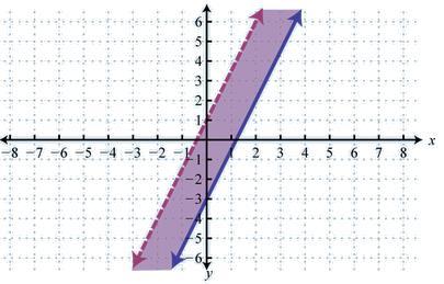
200 Page 200