Imaging, Deconvolution & Image Analysis I. Theory. (IRAM/Obs. de Paris) 7 th IRAM Millimeter Interferometry School Oct. 4 - Oct.

Transcription

1 Imaging, Deconvolution & Image Analysis I. Theory Jérôme PETY (IRAM/Obs. de Paris) 7 th IRAM Millimeter Interferometry School Oct. 4 - Oct , Grenoble

2 Scientific Analysis of a mm Interferometer Output mm interferometer output: Calibrated visibilities in the uv plane ( the Fourier plane). 2 possibilities: uv plane analysis (cf. Lecture by A. Castro-Carrizo): Always better... when possible! (in practice for simple sources as point sources or disks) Image plane analysis: Mathematical transforms to go from uv to image plane! Goal: Understand effects of the imaging process on The resolution; The field of view (single pointing or mosaicing, cf. Lecture by F. Gueth); The reliability of the image; The noise level and repartition (cf. lecture by S.Guilloteau).

3 From Calibrated Visibilities to Images: I. Comparison Visibilities/Source Fourier Transform V ij (b ij ) = 2D FT { B primary.i source } (bij ) + N Primary Beam Distorted source information. Noise Sensitivity problems. Irregular, limited sampling incomplete source information: Support limited at: High spatial frequency limited resolution; Low spatial frequency problem of wide field imaging; Inside the support, incomplete (i.e. Nyquist s criterion not respected) sampling lost of information.

4 From Calibrated Visibilities to Images: II. Effect of Irregular, Limited Sampling Definitions: V = 2D FT { B primary.i source } ; Irregular, limited sampling function: S(u, v) = 1 at (u, v) points where visibilities are measured; S(u, v) = 0 elsewhere; B dirty = 2D FT 1 {S}; I meas = 2D FT 1 {S.V }. Fourier Transform Property #1: I meas = B dirty { B primary.i source }. B dirty : Point Spread Function (PSF) of the interferometer (i.e. if the source is a point, then I meas = I tot.b dirty ).

5 From Calibrated Visibilities to Images: III. Why Deconvolving? Difficult to do science on dirty image. Deconvolution a clean image compatible with the sky intensity distribution.

6 From Calibrated Visibilities to Images: Summary Fourier Transform and Deconvolution: The two key issues in imaging. Stage Implementation Calibrated Visibilities Fourier Transform Dirty beam & image Deconvolution Clean beam & image Visualization Image analysis Physical information on your source GO UVSTAT, GO UVMAP GO CLEAN GO BIT, GO VIEW GO NOISE, GO FLUX, GO MOMENTS

7 From Calibrated Visibilities to Images: Summary Fourier Transform and Deconvolution: The two key issues in imaging. Stage Implementation Calibrated Visibilities Fourier Transform Dirty beam & image Deconvolution Clean beam & image Visualization Image analysis Physical information on your source GO UVSTAT, GO UVMAP GO CLEAN GO BIT, GO VIEW GO NOISE, GO FLUX, GO MOMENTS

8 Direct vs. Fast Fourier Transform Direct FT: Advantage: Direct use of the irregular sampling; Inconvenient: Slow. Fast FT: Inconvenient: Needs a regular sampling Gridding; Advantage: Quick for images of size 2 M 2 N. In practice, everybody use FFT.

9 Gridding: I. Interpolation Scheme Convolution because: Visibilities = noisy samples of a smooth function. Some smoothing is desirable. Nearby visibilities are not independent. V = 2D FT { B primary.i source } = B primary Ĩ source ; FWHM(convolution kernel) < FWHM( B primary ) No real information lost.

10 Gridding: II. Convolution Equation is Kept Through Gridding Demonstration: I grid meas B grid dirty 2D FT G (S.V ) I grid 2D FT G S B grid dirty = G. S; I meas = B dirty { B primary.i source } with I meas = I grid meas/ G and B dirty = B grid dirty / G. meas = G. (S.V ) = G.( S Ṽ ); Remark: Gridding may be hidden in equations but it is still there. Artifacts due to gridding! (cf. next transparencies)

11 Gridding: III. Effect of a Regular Sampling (Periodic Replication) uv Plane Image Plane B primary.i source Regular Sampling function Result for a fine sampling Result for critical sampling (Nyquist s criterion) Result for a coarse sampling

12 Gridding: III. Effect of a Regular Sampling (Aliasing) uv Plane Image Plane Aliasing = Folding of intensity outside the image size into the image. Image size must be large enough.

13 Gridding: IV. Pixel and Image Sizes Pixel size: Between 1/4 and 1/5 of the synthesized beam size (i.e. more than the Nyquist s criterion in image plane to ease deconvolution). Image size: = uv plane sampling rate (FT property # 2); Natural resolution in the uv plane: B primary size; At least twice the B primary size (i.e. Nyquist s criterion in uv plane).

14 Gridding: V. Bright Sources in B primary Sidelobes Bright Sources in B primary sidelobes outside image size will be aliased into image. Spurious source in your image! Solution: Increase the image size. (Be careful: only when needed for efficiency reasons!)

15 Gridding: VI. Noise Distribution

16 Gridding: VII. Choice of Gridding function Gridding function must: Fall off quickly in image plane (to avoid noise aliasing); Fall off quickly in uv plane (to avoid too much smoothing). Define a mathematical class of functions: Spheroidal functions. GILDAS implementation: In GO UVMAP Spheroidal functions = Default gridding function; Tabulated values are used for speed reasons.

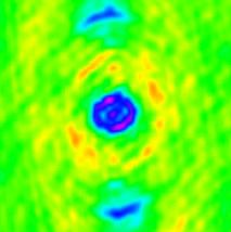
17 Dirty Beam Shape and Image Quality B dirty = 2D FT 1 {S}. Importance of the Dirty Beam Shape: Deconvolving a dirty image is a delicate stage; The closest to a Gaussian B dirty is, the easier the deconvolution; Extreme case: B dirty = Gaussian No deconvolution needed at all! Ways to improve (at least change) B dirty shape: Increase the number of antenna (costly). Change the antenna layout (technically difficult). Weight the irregular, limited sampling function S (the only thing you can do in practice).

18 Dirty Beam Shape and Number of Antenna: 2 Antenna

19 Dirty Beam Shape and Number of Antenna: 3 Antenna

20 Dirty Beam Shape and Number of Antenna: 4 Antenna

21 Dirty Beam Shape and Number of Antenna: 5 Antenna

22 Dirty Beam Shape and Number of Antenna: 6 Antenna

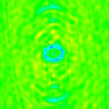
23 Dirty Beam Shape and Super Synthesis

24 Dirty Beam Shape and Super Synthesis

25 Dirty Beam Shape and Super Synthesis

26 Dirty Beam Shape and Super Synthesis

27 Dirty Beam Shape and Super Synthesis

28 Dirty Beam Shape and Super Synthesis

29 Dirty Beam Shape and Super Synthesis

30 Dirty Beam Shape and Super Synthesis

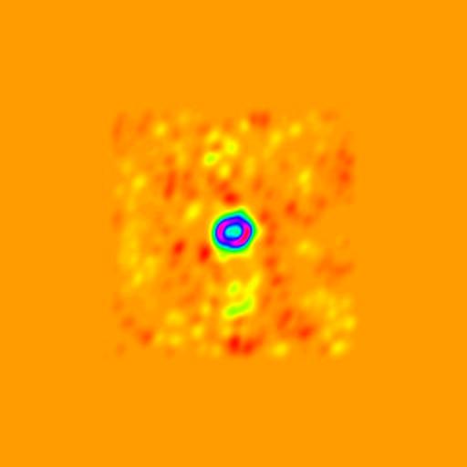
31 Dirty Beam Shape and Weighting Natural Weighting: Default definition of the irregular sampling function at uv table creation. S(u, v) = 1/σ 2 at (u, v) points where visibilities are measured; S(u, v) = 0 elsewhere; with σ 2 (u, v) the noise variance of the visibility. Introduction of a weighting function W (u, v): B dirty = 2D FT 1 {W.S}; Robust weighting: W enhance the large baseline contribution; Tapering: W enhance the small baseline contribution.

32 Definitions: Natural = (u,v) Cell Robust Weighting: I. Definition (u,v) Cell W.S = S; { Constant if (Natural Threshold); Natural else; In practice, the cell size is 0.5D where D is the single-dish antenna diameter (i.e. 15m for PdBI).

33 Robust Weighting: II. Examples

34 Robust Weighting: II. Examples

35 Robust Weighting: II. Examples

36 Robust Weighting: II. Examples

37 Robust Weighting: III. Definition and Properties Definitions: Natural = (u,v) Cell (u,v) Cell S; { Constant if (Natural Threshold); W.S = Natural else; In practice, the cell size is 0.5D. Properties: Increase the resolution; Lower the sidelobes; Degrade point source sensitivity.

38 Tapering: I Definition Definition: Apodization of the uv coverage in general by a Gaussian; ( u 2 + v 2) W = exp where t = tapering distance. t 2 Convolution (i.e. smoothing) of the image by a Gaussian.

39 Tapering: II. Examples

40 Tapering: II. Examples

41 Tapering: II. Examples

42 Tapering: III. Definition and Properties Definition: Apodization of the uv coverage in general by a Gaussian; ( u 2 + v 2) W = exp where t = tapering distance. t 2 Convolution (i.e. smoothing) of the image by a Gaussian. Properties: Decrease the resolution; Degrade point source sensitivity; Increase sensitivity to medium size structures. Inconvenient: Throw out some information. To increase sensitivity to extended sources, use compact arrays not tapering.

43 Weighting and Tapering: Summary Robust Natural Tapering Resolution High Medium Low Side Lobes Medium? Point Source Sensitivity Maximum Extended Source Sensitivity Medium Non-circular tapering: Sometimes Better (i.e. more circular) beams.

44 From Calibrated Visibilities to Images: Summary Fourier Transform and Deconvolution: The two key issues in imaging. Stage Implementation Calibrated Visibilities Fourier Transform Dirty beam & image Deconvolution Clean beam & image Visualization Image analysis Physical information on your source GO UVSTAT, GO UVMAP GO CLEAN GO BIT, GO VIEW GO NOISE, GO FLUX, GO MOMENTS

45 Deconvolution: I. Philosophy Information lost: I meas = B dirty { B primary.i source } + N. Irregular, incomplete sampling convolution by B dirty ; Noise Low signal structures undetected. 1. Impossible to recover the intrinsic source structure! 2. Infinite number of solutions! { } S solution (i.e. Imeas = B dirty S + N) B dirty R = 0 (S +R) solution.

46 Deconvolution: I. Philosophy (continued) I meas = B dirty { B primary.i source } + N. Information lost: 1. Impossible to recover the intrinsic source structure! 2. Infinite number of solutions! Deconvolution goal: Finding a sensible intensity distribution compatible with the intrinsic source one. Deconvolution needs: Some a priori assumptions about the source intensity distribution; As much as possible knowledge of B dirty (OK in radioastronomy); Noise properties. The best solution: A Gaussian B dirty No deconvolution needed!

47 Deconvolution: II. MEM principle a priori assumptions: Smoothed and positive intensity. Idea: Select from the images that agree with the measured visibilities to within the noise level the one that maximizes entropy. Algorithm: Entropy: S = ij I ij log(i ij /M ij ) with M = first guess image. Constraint: k V (u k,v k ) Ĩ(u k,v k ) 2 σ 2 k with Ĩ = 2D FT(I). = number of visibilities

48 Advantages: Deconvolution: II. MEM properties Fast: Computational load N ln(n) with N = number of pixels. Easy to generalize (Arrays with different antenna diameters). Flatten low-level extended emission. Resolve peaks. Inconvenients: Angular resolution increases with peak height. Unable to clean ripples (e.g. point source sidelobes) in extended emission. Biased residuals: Noise increase and spurious emission at low signal. Impossibility to deal with absorption features. Poor performance with limited uv coverage Not used at PdBI.

49 Deconvolution: III. The Basic CLEAN Algorithm a priori assumption: Source = Collection of point sources. Idea: Matching pursuit. Algorithm: 1 Initialize the residual map to the dirty map; the Clean component list to an empty (NULL) value; 2 Identify pixel of I max in residual map as a point source; 3 Add γ.i max to clean component list; 4 Subtract γ.i max from residual map; 5 Go back to point 2 while stopping criterion is not matched; 6 Convolution by Clean beam (a posteriori regularization); 5 Addition of residual map to enable: Correction when cleaning is too superficial; Noise estimation.

50 Deconvolution: III. The Basic Clean Algorithm 1. First Illustration

51 Deconvolution: III. The Basic Clean Algorithm 1. First Illustration

52 Deconvolution: III. The Basic Clean Algorithm 1. First Illustration

53 Deconvolution: III. The Basic Clean Algorithm 1. First Illustration

54 Deconvolution: III. The Basic Clean Algorithm 1. First Illustration

55 Deconvolution: III. The Basic Clean Algorithm 1. First Illustration

56 Deconvolution: III. The Basic Clean Algorithm 1. First Illustration

57 Deconvolution: III. The Basic Clean Algorithm 1. First Illustration

58 Deconvolution: III. The Basic Clean Algorithm 1. First Illustration

59 Deconvolution: III. The Basic Clean Algorithm 1. First Illustration

60 Deconvolution: III. The Basic Clean Algorithm 1. First Illustration

61 Deconvolution: III. The Basic Clean Algorithm 2. Second Illustration

62 Deconvolution: III. The Basic Clean Algorithm 2. Second Illustration

63 Deconvolution: III. The Basic Clean Algorithm 2. Second Illustration

64 Deconvolution: III. The Basic Clean Algorithm 2. Second Illustration

65 Deconvolution: III. The Basic Clean Algorithm 2. Second Illustration

66 Deconvolution: III. The Basic Clean Algorithm 2. Second Illustration

67 Deconvolution: III. The Basic Clean Algorithm 2. Second Illustration

68 Deconvolution: III. The Basic Clean Algorithm 2. Second Illustration

69 Deconvolution: III. The Basic Clean Algorithm 2. Second Illustration

70 Deconvolution: III. The Basic Clean Algorithm 2. Second Illustration

71 Deconvolution: III. The Basic Clean Algorithm 3. Little Secrets Convergence: Too superficial cleaning Approximate results. Too deep cleaning Divergence.

72 Deconvolution: III. The Basic Clean Algorithm 3. Little Secrets Addition of residual map: Improvement when convergence not reached; Noise estimation.

73 Deconvolution: III. The Basic Clean Algorithm 3. Little Secrets Addition of residual map: Improvement when convergence not reached; Noise estimation.

74 Deconvolution: III. The Basic Clean Algorithm 3. Little Secrets Choice of clean beam: Gaussian of FWHM matching the synthesized beam size. Super resolution strongly discouraged.

75 Deconvolution: III. The Basic Clean Algorithm 3. Little Secrets Negative clean components are mandatory.

76 Deconvolution: III. The Basic Clean Algorithm 3. Little Secrets Negative clean components are mandatory.

77 Deconvolution: III. The Basic Clean Algorithm 3. Little Secrets Negative clean components are mandatory.

78 Deconvolution: III. The Basic Clean Algorithm 3. Little Secrets Negative clean components are mandatory.

79 Deconvolution: III. The Basic Clean Algorithm 3. Little Secrets Negative clean components are mandatory.

80 Deconvolution: III. The Basic Clean Algorithm 3. Little Secrets Negative clean components are mandatory.

81 Deconvolution: III. The Basic Clean Algorithm 3. Little Secrets Negative clean components are mandatory.

82 Deconvolution: III. The Basic Clean Algorithm 3. Little Secrets Negative clean components are mandatory.

83 Deconvolution: III. The Basic Clean Algorithm 3. Little Secrets Negative clean components are mandatory.

84 Deconvolution: III. The Basic Clean Algorithm 3. Little Secrets Negative clean components are mandatory.

85 Deconvolution: III. The Basic Clean Algorithm 4. Other Little Secrets Stopping criterions: Total number of Clean components; I max < fraction of noise (when noise limited); I max < fraction of dirty map max (when dynamic limited). Loop gain: Good results when γ Cleaned region: Only the inner quarter of the dirty image. Support: searched. Definition of a region where CLEAN components are A priori information Help CLEAN convergence. But bias if support excludes signal regions Be wise!

86 Deconvolution: III. The Basic Clean Algorithm 5. A True Example without support

87 Deconvolution: III. The Basic Clean Algorithm 5. A True Example without support (zoom)

88 Deconvolution: III. The Basic Clean Algorithm 5. A True Example with right support

89 Deconvolution: III. The Basic Clean Algorithm 5. A True Example with wrong support

90 Deconvolution: IV. CLEAN Variants Basic: HOGBOM (Hogböm 1974) Robust but slow. Faster Search Algorithms: CLARK (Clark 1980) Fast but instable (when sidelobes are high). MX (Cotton& Schwab 1984) Better accuracy (Source removal in the uv plane), but slower (gridding steps repeated). Better Handling of Extended Sources: MULTI (Multi-Scale Clean by Cornwell 1998) Multi-resolution approach.

91 Deconvolution: IV. CLEAN Variants (continued) Exotic use at PdBI: SDI (Steer, Dewdney, Ito 1984) Created to minimize stripes. MRC (Multi-Resolution Clean by Wakker & Schwarz 1988) Too simple multi-resolution approach.

92 Deconvolution: V. Recommended Practices Method: Start with CLARK and turn to HOGBOM in case of high sidelobes. Support: Start without one. Define one on your first clean image if really needed (i.e. difficulties of convergence). Stopping criterion: Use a large enough number of iterations to ensure convergence. Clean down to the noise level unless a very strong source is present. Misc: Consult an expert until you become one.

93 Visualization and Image Analysis Fourier Transform and Deconvolution: The two key issues in imaging. Stage Implementation Calibrated Visibilities Fourier Transform Dirty beam & image Deconvolution Clean beam & image Visualization Image analysis Physical information on your source GO UVSTAT, GO UVMAP GO CLEAN GO BIT, GO VIEW GO NOISE, GO FLUX, GO MOMENTS

94 Photometry: I Generalities Brightness = Intensity (e.g. Power = I ν (α, β)dadωdν) Flux unit: 1 Jy = W m 2 Hz 1. Source flux measured by a single dish antenna: F ν = B I ν with B the antenna beam. Relationship between measured flux and temperature scales: T A = 2kΩ λ2 F ν, T A A = 2kΩ λ2 F ν and T 2π mb = 2kΩ λ2 F ν because mb P ν = 1 2 A ef ν Power detected by the single dish antenna. P ν = kt Power emitted by a resistor at temperature T. P ν = P ν T A = A e 2k F ν. λ 2 = A e Ω A (diffraction). Ω 2π = F eff Ω A or F eff = Forward beam Total beam. Ω mb = B eff Ω A or B eff = Main beam Total beam.

95 Photometry: II Visibilities Visibility unit: Jy because: V = 2D FT { B primary.i source } = B primary (σ).i source (σ) exp( i2πb.σ/c)dω. Effect of flux calibration errors on your image: Multiplicative factor if uniform in uv plane. Convolution (i.e. distorsion) else.

96 Photometry: III Dirty map Ill defined because: S(u = 0, v = 0) = 0 Area of the dirty beam is 0! V (u = 0, v = 0) = 0 Total flux of the dirty image is 0! A source of constant intensity will be fully filtered out. A single point source of 1 Jy appears with peak intensity of 1. Several close-by point sources of 1 Jy appears with peak intensities different of 1.

97 Photometry: IV Clean map (my dream: Don t take it seriously) I clean = 1 Ω clean ( Bclean I point ) : i.e. convolution of a set of point sources (mimicking the sky intensity distribution) by the clean beam. Behavior: Brightness, i.e. Source flux measured in a given solid angle (i.e. 1 steradian). Unit: Jy/sr Consequences: Source flux computation by integration inside a support: Flux = [Jy] ij S with dω the image pixel surface. I clean dω [Jy/sr] [sr] From Brightness to temperature: T clean = λ2 2k I clean

98 Photometry: IV Clean map (reality) I clean = B clean I point : i.e. convolution of a set of point sources (mimicking the sky intensity distribution) by the clean beam. Behavior: Brightness, i.e. Source flux measured in a given solid angle (i.e. clean beam). Unit: Jy/beam with 1 beam = Ω clean sr. Consequences: Source flux computation by integration inside a support: Flux = [Jy] ij S I clean. dω Ω clean [Jy/beam] [beam] with dω Ω clean the nb of beams in the surface of an image pixel. From Brightness to temperature: T clean = λ2 2kΩ clean I clean

99 Photometry: IV Clean map Consequences of a Gaussian clean beam shape: No error beams, no secondary beams. T clean is a main beam temperature. Natural choice of clean beam size: Synthesized beam size (i.e. fit of the central peak of the dirty beam). Minimize unit problems when adding the dirty map residuals. Caveats of flux measurements: CLEAN does not conserve flux (i.e. CLEAN extrapolates unmeasured short spacings). Large scales are filtered out (source size > 1/3 primary beam size need of short spacings, cf. lecture by F. Gueth). I clean = B primary.i source + N Primary beam correction may be needed: I clean /B primary = I source + N/B primary Varying noise! Seeing scatters flux.

100 Photometry: V Importance of Extended, Low Level Intensity

101 Noise: I. Formula δt = λ2 2k σ Ω with σ = 2k η T sys t ν N ant (N ant 1)A δt Brightness noise [K]. λ Wavelenght. k Boltzmann constant. Ω Synthesized beam solid angle. A Antenna area. σ Flux noise [Jy]. T sys System temperature. t On-source integration time. ν Channel bandwidth. N ant Number of antennas. and η Global efficiency ( = Quantum x Antenna x Atm. Decorrelation).

102 Noise: II. σ to compare instruments δt = λ2 2k σ Ω with σ = 2k η T sys t ν N ant (N ant 1)A Wavelenght: 1 mm. T sys = 150 K. Decorrelation = 0.8. Instrument Bandwidth σ On-source time PdBI GHz 1.0 mjy/beam 3 min ALMA GHz 1.0 mjy/beam 3 sec ALMA GHz 0.12 mjy/beam 3 min One order of magnitude ( 8 ) sensitivity increase in continuum.

103 Noise: III. δt to prepare observations: 1. Continuum δt = λ2 2k σ Ω with σ = 2k η T sys t ν N ant (N ant 1)A Wavelenght: 1 mm. T sys = 150 K. Decorrelation = 0.8. Instrument Bandwidth Resol. δt On time Comment PdBI GHz mk 3 hrs ALMA GHz mk 3 min Low contrast, many objects ALMA GHz mk 3 hrs High contrast, same object ALMA GHz mk 500 hrs 5.7% of a civil year ALMA GHz mk 3 hrs Intermediate sensitivity ALMA GHz mk 3 hrs Intermediate resolution Almost one order of magnitude ( 8 ) sensitivity increase A factor 3 resolution increase (same integration time, same noise level). Wolf et al. 2002, 0.02 in 3 hrs.

104 Noise: III. δt to prepare observations: 2. Line δt = λ2 2k σ Ω with σ = 2k η T sys t ν N ant (N ant 1)A Channel width: 0.8 km s 1. Wavelenght: 1 mm. Decorrelation = 0.8. Instrument Resolution δt On-source time Comment PdBI now K 2 hrs ALMA K 3.5 min Same line, many objects ALMA K 2 hrs Fainter lines, same objec ALMA K 575 hrs 6.5% of a civil year! ALMA K 2 hrs Intermediate sensitivity ALMA K 2 hrs Intermediate resolution A factor 6 sensitivity increase A factor 2.4 resolution increase (same integration time, same noise level).

105 Noise: IV. Advices δt = λ2 2k σ Ω with σ = 2k η T sys t ν N ant (N ant 1)A For your estimation: Use a sensitivity estimator! The estimator is probably optimistic! Use δt not σ.

106 Writing the Paper: Your job!

107 Mathematical Properties of Fourier Transform 1 Fourier Transform of a product of two functions = convolution of the Fourier Transform of the functions: If (F 1 FT F 1 andf 2 FT F 2 ), then F 1.F 2 FT F 1 F 2. 2 Sampling size FT Image size. 3 Bandwidth size FT Pixel size. 4 Finite support FT Infinite support. 5 Fourier transform evaluated at zero spacial frequency = Integral of your function. V (u = 0, v = 0) FT ij image I ij.

108 Photographic Credits and References R. N. Bracewell, The Fourier Transform and its Applications. J. D. Kraus, Radio Astronomy. R. Narayan and R. Nityananda, Ann. Rev. Astron. Astrophys., 1986, 24, , Maximum Entropy Image Restoration in Astronomy