Comparison of concrete rheometers: International tests at LCPC (Nantes, France) in October, 2000

Transcription

1 NISTIR 6819 Comparison of concrete rheometers: International tests at LCPC (Nantes, France) in October, 2 Editors: Chiara F. Ferraris, Lynn E. Brower Authors (alphabetical order): Phil Banfill, Denis Beaupré, Frédéric Chapdelaine, François de Larrard, Peter Domone, Laurent Nachbaur, Thierry Sedran, Olaf Wallevik, Jon E. Wallevik

2 NISTIR 6819 Comparison of concrete rheometers: International tests at LCPC (Nantes, France) in October, 2 Editors: Chiara F. Ferraris, National Institute of Standards and Technology (USA) Lynn E. Brower, Master Builders Technologies (USA) Authors (in alphabetical order): Phil Banfill, Heriot-Watt Univ., (UK) Denis Beaupré, Laval Univ., (Canada) Frédéric Chapdelaine, Laval Univ (Canada) François de Larrard, Laboratoire Central des Ponts et Chaussées, (France) Peter Domone, University College London (UK) Laurent Nachbaur, Laboratoire Central des Ponts et Chaussées, (France) Thierry Sedran, Laboratoire Central des Ponts et Chaussées, (France) Olaf Wallevik, The Icelandic Building Research Institute, (Iceland) Jon E. Wallevik, Norwegian Univ. of Science and Technology, (Norway) September 21 U.S. Department of Commerce Donald L. Evans, Secretary National Institute of Standards and Technology Karen H. Brown, Acting Director

3 Disclaimer Commercial equipment, instruments, and materials mentioned in this paper are identified to foster understanding. Such identification does not imply recommendation or endorsement by the National Institute of Standards and Technology (NIST), nor does it imply that the materials or equipment identified are necessarily the best available for the purpose. During the trial in France, on October 2, to ensure proper use, each designer operated his instrument and described its operation in this report. All data were immediately, after each test, collected in electronic form on specially labeled diskettes for later analysis. The role of NIST was to coordinate and foster the rheometer study. Dr. Chiara Ferraris is the chair of ACI 236A, Workability of Fresh Concrete, and in this role she organized the tests and edited the report. She is not one of the authors, but only an editor. Lynn Brower, co-editor, is the secretary of ACI 236A. The opinions expressed in this report are not endorsed by NIST and they reflect only the opinion of the authors.

4 Preparation of the report Editors Chiara F. Ferraris, National Institute of Standards and Technology, Gaithersburg (USA) Lynn Brower, Master Builders, Inc., Cleveland OH (USA) Authors (alphabetical order) Phil Banfill, Heriot-Watt Univ., Edinburgh (UK) Denis Beaupré, Laval Univ., Quebec (Canada) Frédéric Chapdelaine, Laval Univ., Quebec (Canada) François de Larrard, Laboratoire Central des Ponts et Chaussées, Nantes (France) Peter Domone, University College London (UK) Laurent Nachbaur, Laboratoire Central des Ponts et Chaussées, Paris (France) Thierry Sedran, Laboratoire Central des Ponts et Chaussées, Nantes (France) Olaf Wallevik, The Icelandic Building Research Institute, Reykjavik (Iceland) Jon E. Wallevik, Norwegian Univ. of Science and Technology, Trondheim (Norway) Contact Chiara F. Ferraris NIST 1 Bureau drive, MS 8621, Gaithersburg MD 2899 (USA) Phone: Fax: clarissa@nist.gov

5 Participants in the tests at LCPC, Nantes (France) 1 st row: left to right Jean-Yves Petit, Jinhua Jin, Jon Wallevik, Daniel Michel, Francois de Larrard, Chiara Ferraris, Olafur Wallevik, Marie-Andrée Gilbert, Thierry Sedran, Frederic Chapdelaine, Mohammed Sonebi, Joseph Daczko 2 nd Row: left to right Alain Doucet, Michel Dauvergne, Pierre Chelet (behind Michel), Bernard Dehousse, Phil Banfill, Peter Domone, Andreas Griesser, Laurent Nachbaur, Erik Nordenswan On top of the CEMAGREF-IMG: Denis Beaupré Affiliations of participants (in alphabetical order): Addtek, Parainen (Finland): Erik Nordenswan Advanced Concrete and Masonry Centre, Paisley (UK): Mohammed Sonebi Heriot-Watt Univ., Edinburgh (UK): Phil Banfill, Jinhua Jin The Icelandic Building Research Institute, Reykjavik (Iceland): Olaf Wallevik Laboratoire Central des Ponts et Chaussées, Nantes (France): François de Larrard, Thierry Sedran, Alain Doucet, Michel Dauvergne, Pierre Chelet, Bernard Dehousse, Daniel Michel Laboratoire Central des Ponts et Chaussées, Paris (France): Laurent Nachbaur Laval Univ., Quebec (Canada): Denis Beaupré, Frédéric Chapdelaine, Marie-Andrée Gilbert National Institute of Standards and Technology, Gaithersburg (USA): Chiara F. Ferraris Norwegian Univ. of Science and Technology, Trondheim (Norway): Jon E. Wallevik Univ. d Artois, Bethune (France): Jean-Yves Petit University College London (UK): Peter Domone Master Builders, Inc., Cleveland OH (USA): Joseph Daczko Swiss Federal Institute of Technology, Zürich (Switzerland): Andreas Griesser

6 Foreword The American Concrete Institute (ACI) sub-committee 236A, Workability of Fresh Concrete, immediately was faced, upon its creation in fall 1999, with how to determine appropriate methods to measure concrete workability. The material sciencebased approach to measure workability would be to use a concrete rheometer. There are several rheometers used around the world that have significant design differences, but no standard method with which to compare their results. ACI 236A members determined that, as no reference material was available, one method to compare the rheometers would be to test them under the same conditions using the same concretes. Some tentative analysis made to compare two rheometers was performed in the past [1, 2] but did not involve most of the available rheometer designs. ACI 236A drafted a plan for comparing the five types of rheometers available and requested funds from the Concrete Research Council (CRC) of ACI and from industry to support this work. CRC granted funds in 2 and the first trial was scheduled for October, 2. It was held at the Laboratoire Central des Ponts et Chaussées (LCPC) facility in Nantes, France on October 23-27, 2. The rheometers selected included all commercially available concrete rheometers (four), to the best knowledge of the ACI 236A committee members, and one coaxial concrete rheometer developed for research. The authors of this report are principal investigators who participated in the first trial and contributed to the report. This report describes the tests performed and the results obtained. It was not published as an ACI document and therefore was not submitted to the Technical Activities Committee (TAC) for approval. There are two reasons for this not being an ACI document: 1) ACI documents are guidelines and practice recommendations, not research reports; 2) all ACI reports are consensus documents balloted and approved by the members of a committee, while this report only reflects the views and opinions of the authors. All members of ACI 236A were invited to review the document prior to publication (as shown in the acknowledgements). It was also discussed during the regular meetings of ACI 236A at the ACI spring 21 convention in Philadelphia (PA).

7 Acknowledgements This project could not have been possible without the financial support of the ACI Concrete Research Council. Its support offset the cost of the transportation of the rheometers from Canada, Switzerland, UK, and Grenoble (France) to the test site at Laboratoire Central des Ponts et Chaussées (LCPC) in Nantes (France). We are thankful for the hospitality and the professionalism of the staff of LCPC, who welcomed the international team for the week-long tests. We would like to acknowledge the participation of LCPC staff, in particular: Michel Dauvergne, Daniel Michel, Alain Doucet, Pierre Chelet, Bernard Dehousse, David Chopin and Bernard Guieysse. They prepared and tested all the concrete used for this project, and conducted all the concrete quality control measurements. We would also like to thank all the participants and their organizations for their involvement in the planning and execution of this comparison. Their names are listed in the participants list placed before the foreword. Also, Master Builders Technology (MBT) should be thanked for providing their expertise to administer the funds provided by CRC. The authors would also like to thank all the reviewers for their efforts in reading this rather large report (in alphabetical order): Emmanuel Attiogbe (MBT), Samir Chidiac (McMaster Univ.), Geoffrey Fronhsdorff (NIST), Edward Garboczi (NIST), Aulis Kappi (Addtek R&D), Nicos Martys (NIST), Abdelbaki Mekhatria (CRIB, Laval Univ.), Della Roy (Penn State Univ.), Leslie Struble (ACBM, Univ. of Illinois), Kejin Wang (Iowa State Univ.), and Walter Rossiter (NIST). We would also like to thank the members of ACI 236A for their lively discussion during the Spring 21 meeting and their support of this study.

8 Table of Contents 1. INTRODUCTION CONCRETE MIXTURES USED IN TESTS AT NANTES CONSTITUENTS MIXTURE PROPORTIONS CONCRETE PRODUCTION FRESH CONCRETE ANALYSES CONCRETE RHEOMETERS THE BML RHEOMETER Description of apparatus Test procedures Calibration THE BTRHEOM RHEOMETER Description of the apparatus Test procedure Analysis of the data THE CEMAGREF-IMG RHEOMETER Description of the apparatus Test procedure Analysis of the data THE IBB RHEOMETER Description of the apparatus Analysis of the data THE TWO-POINT RHEOMETER Description of the apparatus Test procedure Analysis of the data RESULTS QUALITY CONTROL MEASUREMENTS: SLUMP, MODIFIED SLUMP, DENSITY COMPARISON BETWEEN RHEOMETERS Comparison with the slump and modified slump test Variation of the values by concrete composition Analysis of variation of the yield stress and plastic viscosity by mixture Relative rank of the data by each rheometer Graphical comparison of pairs of rheometer results Correlation functions and coefficients between pairs of rheometers DISCUSSION COMMENTS ON CORRELATIONS BETWEEN PAIRS OF RHEOMETERS Linear regression or not? Critical review of R DISCUSSION ON DISCREPANCIES ON ABSOLUTE VALUES CORRELATION BETWEEN THE SLUMP AND THE YIELD STRESS SUMMARY OF FINDINGS FUTURE WORK REFERENCES APPENDIXES.A-69

9 List of Figures Figure 1: Size distributions of the aggregates used...3 Figure 2: The ConTec viscometers: a) Version 3; b) Version Figure 3: Output from the FreshWin software: A) The menu-driven window used to change relevant parameters; B) The basic output of a test result...12 Figure 4: The inner and outer cylinder of the BML Viscometer 3 (or BML rheometer hereafter) Figure 5: The assembly of inner cylinder of the BML viscometer 3. This figure shows the sequence for installing the inner cylinder Figure 6: A top view of a coaxial cylinder rheometer. The outer cylinder (radius r o ) rotates at angular velocityω o, while the inner cylinder (radius r i ) is stationary and registers the torque transferred through the fluid material...15 Figure 7: The relation between torque measured by the rheometer and shear stress...17 Figure 8: Output from the software during calibration of the BML rheometer...18 Figure 9: Principle of the BTRHEOM rheometer...19 Figure 1: The BTRHEOM rheometer showing the blades at the top and bottom of the bucket containing the concrete...21 Figure 11: Schematic of the CEMAGREF-IMG rheometer...22 Figure 12: Picture of the CEMAGREF-IMG rheometer...23 Figure 13: Top view of the CEMAGREF-IMG rheometer with grid on the inner cylinder and blades on the outer one...23 Figure 14: Sketch showing set-up of the calibrated load cells to measure the torque...24 Figure 15: Description of the speed-meter...25 Figure 16: Diagram of plug flow phenomenon...26 Figure 17: Typical curves versus time obtained during a test...29 Figure 18: Torque-rotation speed curve for the same test as in Figure Figure 19: The IBB Rheometer...3 Figure 2: Details of the H-shaped impellers, bowls and planetary motion for IBB rheometer for concrete (a) and mortar (b). Dimension in mm...31 Figure 21: Example of calculation with indication of the meaning of the parameters. Y= speed; x = Torque...32 Figure 22: Impeller and bowl dimensions (in mm)...33 Figure 23: The overall arrangement of the Two-Point test apparatus...34 Figure 24: Comparison of the slumps measured by the standard method and the modified method. The dotted line represents the 45 line Figure 25: Comparison of standard slump and yield stress as measured with the five rheometers. The second axis in N m gives the results obtained with the IBB....4 Figure 26: Comparison of plastic viscosity calculated from the modified slump test and plastic viscosity as measured with the five rheometers. The second axis in N m s gives the results obtained with the IBB Figure 27: Comparison of the yield stresses as measured with the rheometers...42 Figure 28: Comparison of the plastic viscosities as measured with the rheometers...42 Figure 29: Comparison between BML and BTRHEOM...48 Figure 3: Comparison between BML and CEMAGREF-IMG...49 Figure 31: Comparison between BML and IBB...5 Figure 32: Comparison between BML and Two-Point test...51 Figure 33: Comparison between BTRHEOM and CEMAGREF-IMG...52 Figure 34: Comparison between BTHEOM and IBB...53 Figure 35: Comparison between BTRHEOM and Two-Point test...54 Figure 36: Comparison between IBB and CEMAGREF-IMG...55 Figure 37: Comparison between CEMAGREF-IMG and Two-Point test...56 Figure 38: Comparison between IBB and Two-Point test...57 Figure 39: Comparison of plastic viscosities between BML, BTRHEOM and Two-Point test when the data points from Mixture #4 were omitted...58

10 Figure 4: Comparison of plastic viscosities between IBB and Two-Point test. The data from Mixture #4 were omitted...59 Figure 41: Comparison of measured and predicted yield stress according to equations developed by Hu and Kurakawa...63 List of Tables Table 1: Compositions of mixtures (in kg/m 3 ) produced with crushed 5/16 mm coarse aggregate in the mixing plant during the rheology week...6 Table 2: Compositions of mixtures (in kg/m 3 ) produced with rounded 4/2 mm coarse aggregate on the mixing plant during the rheology week...6 Table 3: Composition of a mixture (in kg/m 3 ) produced with crushed /6.3 mm coarse aggregate in the mixing plant during the rheology week...7 Table 4: Fresh concrete analyses. Mixtures # Table 5: Fresh concrete analyses. Mixtures # 5-7 & Table 6: Fresh concrete analyses. Mixtures # Table 7: Dimensions of the inner and outer cylinders of the five standard measuring systems. The configuration used in the tests presented here is highlighted in gray...12 Table 8: Slump Measurements...38 Table 9: Yield stress and viscosities calculated from the measurements...39 Table 1: Ranking of the yield stresses of the mixtures as determined by the rheometers and the slump. The mixtures are ranked in decreasing order of yield stress from 1 to 12. The higher the slump, the lower the yield stress...44 Table 11: Ranking of the plastic viscosity of the mixtures as determined by the rheometers. The mixtures are ranked in decreasing order of plastic viscosities from 1 to Table 12: Correlation coefficients for yield stress...46 Table 13: Correlation coefficients for plastic viscosity...46 Table 14: Correlation coefficients for plastic viscosity if Mixture #4 for Two-Point test is not considered (see text for rationale)...46 Table 15: Between-rheometer linear correlation functions for the yield stress. The rheometers in the column head are Y and those in the row head are X. In each cell the coefficients of the equation Y=AX +B are shown. The rheometers are listed in alphabetical order...47 Table 16: Between-rheometer linear correlation functions for the plastic viscosity (all data available are used). The rheometers in the column head are Y and those in the row head are X. In each cell the coefficients of the equation Y=AX +B are shown. The rheometers are listed in alphabetical order...47 Table 17 Critical values for the correlation coefficient R of a sample extracted from a normal distributed population. α is the probability, and ν = n-2, n being the number of points. If the calculated value of R is higher than the reference value shown in the table, there is a probability α that X and Y are dependent...61

11 1. Introduction Concrete is a complex material and its properties in the fresh state can have a large effect on hardened properties. Unfortunately, the technology to measure the properties of fresh concrete has not changed significantly in the last century. The main fresh concrete property, workability, is still measured using the slump test (ASTM C 143). In fact, concretes with the same slump may flow differently and have different workability [3, 4]. The reason two concretes with the same slump behave differently during placement is that concrete flow cannot be defined by a single parameter. Most researchers agree that the flow of concrete can be described reasonably well using a Bingham equation. This equation is a linear function of the shear stress (the concrete response) versus shear rate. Two parameters provided by the Bingham equation are the yield stress and the plastic viscosity. The yield stress correlates reasonably well with the slump value, but the plastic viscosity is not measured at all using the slump test. Plastic viscosity governs concrete flow behavior after flow has started, i.e., after the yield stress is overcome. The existence of the plastic viscosity helps explain why concretes with the same slump may behave differently during placement. It is critical to completely define concrete flow when special concretes, demanding major control of workability, such as a self-compacting concrete (SCC) or high performance concrete (HPC), are used or when concrete is placed in highly-reinforced structures [5]. This is critical because a single parameter such as the slump does not adequately describe their behavior during placement. More sophisticated and precise tools are needed to determine the workability or flow properties of such concretes. Several instruments have been designed to address this problem [6], some in an empirical manner, and some attempting to apply absolute physical measurements to concrete rheology, i.e., fluid rheology. The devices attempting to use fluid rheology methods to measure the flow of concrete, i.e., measuring shear stress at varying shear rates, are called rheometers [7]. They all measure the resistance to flow of concrete at varying shear rate conditions. Rheometers designed for polymers or neat fluids with no solid particles are not suitable for measuring concrete due to the presence and size of the solid aggregates. This situation has lead to a wide variety of designs for concrete rheometers, making it difficult if not impossible to compare the results of the rheometers on a common basis. One obvious solution would be to have a standard reference material to calibrate the rheometers. No such standard material has been developed to simulate fresh concrete behavior. Therefore, the best alternative was to conduct measurements using the rheometers on the same concrete mixtures. The first project goal was to compare the data measured by the various devices. If these measurements differed significantly, the second goal was to establish correlation functions between the rheometer results to make possible reasonable comparisons of data obtained with different rheometers. The concrete rheometers that are available today and were used in this study are: BML (Iceland) [8, 9] BTRHEOM (France) [1, 11] CEMAGREF-IMG coaxial rheometer (France) [1] 1

12 IBB (Canada) [12] Two-Point (UK) [13] The IBB and Two-Point rheometers are based on rotating an impeller in fresh concrete contained within a cylindrical vessel. The shape of the vane varies with the rheometer. The speed of rotation of the blade is increased and then decreased while the concrete resistance or torque is measured. The BTRHEOM is a parallel plate rheometer. The concrete is placed in a cylindrical container with a fixed bottom plate. A top plate embedded in the concrete is rotated at increasing and then decreasing speeds and the torque is measured. The CEMAGREF-IMG and the BML are coaxial cylinder rheometers in which one cylinder (inner cylinder for the CEMAGREF-IMG and outer for the BML) is rotated at increasing and decreasing speed and the torque induced by the concrete on the inner cylinder is measured. The flow pattern of the concrete in the IBB and Two- Point rheometers cannot be easily assessed or modeled, while the flow can be mathematically modeled for the coaxial rheometers (BML, CEMAGREF-IMG) and for the parallel-plate rheometer (BTRHEOM). For these three rheometers (BML, BTRHEOM, CEMAGREF-IMG), rheological characteristics in fundamental units can be calculated. The Two-Point test rheometer requires indirect methods using calibrating fluids of known viscosity to convert quantitative data into the fundamental units needed. On the other hand, the IBB is not calibrated with a fluid and therefore, the results are not reported in fundamental units. The aim of the present project was to compare measurements from these five rheometers to provide data to establish correlations among them. Differences between the various rheometers were expected, due to the complex granular structure of concrete. Slip at the rheometer surfaces and coarse particle segregation are just two examples of such granular aspects of fresh concrete behavior. They are not accounted for in rheometer analyses, that are based upon classical fluid mechanics of homogeneous fluids. Comparison and correlation functions, which can relate the results obtained with the various rheometers, are essential to advance the science of concrete rheology and therefore provide a better characterization of concrete workability. Under the auspices of ACI sub-committee 236A, Workability of Fresh Concrete, a group of researchers obtained a grant from ACI s Concrete Research Council (CRC) to conduct a series of comparison tests on concrete rheometers. The first test was conducted on October 23-27, 2 in the facilities of the Laboratoire Central des Ponts et Chaussées (LCPC) located in Nantes (France). This report describes the rheometers used and their operation, the concrete compositions and preparation procedure, and all the data obtained as well as some data interpretation of this. All the data are presented as measured. This will provide a valuable database for use by researchers in this field. Summaries of the different aspects of this research along with further analysis, will be presented in ACI journals and other publications. 2

13 2. Concrete Mixtures Used in Tests at Nantes 2.1. Constituents Twelve mixtures were produced with local materials from the Nantes area. The cement was a CPA CEM I 52.5 from Saint-Pierre la Cour (equivalent to an ASTM type I). For the self-compacting mixtures, a Piketty limestone filler was added. A densified silica fume from Anglefort was used in some concretes for which both low yield stress and low plastic viscosity was required. Most mixtures used a high-range water reducer (HRWRA), which was either a polycarboxylate (commercial name: MBT Glenium 27 ) or a sulphonated melamine (Commercial name: Chryso Résine GT ). A viscosity agent (Commercial name: MBT Meyco MS685, a suspension of amorphous precipitated nanosilica) was added to the self-compacting mixtures. Tap water was used for all mixtures. Up to four different aggregate fractions were used for each concrete, to obtain the best possible control of the aggregate size distribution. All concretes contained the same sand, a /4 (from mm to 4 mm) Estuaire sand (from the Loire river). In addition, some mixtures also used a very fine (correcting) sand called /.4 from Palvado, to maintain a continuous distribution between the cement and the aggregate size ranges. Mixtures #1-7 were made with two fractions of crushed coarse aggregate (gneiss from the Pontreaux quarry, with a maximum size of 16 mm). Mixtures # 8-11 contained a rounded silico-calcareous river gravel (also in two fractions) from Longué (Vienne river), with a maximum size of 2 mm. Finally, the last mixture #12 only contained a small crushed aggregate from Pontreaux with a maximum size of 6.3 mm. Size distributions of all agregates are displayed in Figure 1. % passing Limestone Filler Portland Cement Palvado /.4 Estuaire /4 Pontreaux 2/6.3 Longué 4/ Pontreaux 5/12.5 Pontreaux 1/16 Longué 1/2 d (mm) Figure 1: Size distributions of the aggregates used 3

14 2.2. Mixture proportions The mixtures were designed with the help of LCPC mixture-design software BétonlabPro 2 [14]. The objective was to obtain a broad range of combinations of yield stress and plastic viscosity, while minimizing the tendency to segregation. This strategy was followed for #1-4 and #8-11 mixtures. The main difference between these two series was the nature of the coarse aggregate. Since the goal of this rheology project was to test the correlation between a variety of devices, it was useful to see whether such correlations would hold for different types of aggregate. Repetitions of mixtures were planned if time allowed. Mixture #5 was a gap-graded mixture, with the high coarse/fine aggregate ratio slightly higher than most mix-design method recommendations. The idea was to generate a concrete in which mortar and coarse aggregate would have a tendency to separate from each other, but would not display any obvious segregation in the normal operations of mixing, discharging and casting. Mixtures #6-7 were planned to be self-compacting mixtures, with very low yield stress, moderate plastic viscosity and high stability at rest and during casting in congested areas. Both mixtures had the same dry composition, differing only in the water and superplasticizer dosages. Finally, mixture # 12 was a high-performance micro-concrete made with a very small aggregate (having a maximum size of 6.3 mm), with a high amount of fines, a low yield stress and a moderate plastic viscosity. Although the test of this concrete was not originally intended, it was considered interesting to include it, because this mixture was designed to minimize the wall effects and segregation in the various rheometers. Before the testing date, all mixtures were prepared and adjusted in the laboratory, on the basis of 4 L batches produced with a 12 L pan mixer Concrete production Between development of the mixtures in the laboratory and production at the concrete plant, the cement silo was filled with a new delivery of portland cement (from the same manufacturer). Also, the various aggregate fractions were stored outside, so that aggregate water content varied widely during the project. Concretes were produced at the Mixing Study Station of LCPC, Nantes (see figure in Appendix A). This station is devoted to research on the production of granular cold material (like concrete and various road base materials) on an industrial scale. A variety of mixers can be mounted on the station, which incorporates all ordinary facilities for storing, weighing and batching materials with suitable automation. For this project, a 1 m 3 pan-mixer was used. In order to control the water content of the concretes, the sand fractions were first weighed and batched into the mixer. The sand fractions could contribute the largest error 4

15 in the water content of the concrete. After some minutes of mixing, a sample of the sand was taken to measure the water content. Then, the masses to be added in order to control the proportions of the mixture were calculated, and all the other materials were batched, including coarse aggregate fractions, cement and other binders if any, and finally the rest of water incorporating one third of the total superplasticizer amount. The rest of the superplasticizer was added later as needed. Due to changes in material batches, sand water content, and batch size, the workability of the concretes often differed from that originally obtained in the lab. In order to avoid production of unsuitable mixtures, the mixing process was systematically interrupted, and the concrete sampled to make a slump test. Based on this slump indication, supplementary additions of water and/or superplasticizer were made as needed. Then mixing was restarted and stopped after a while to check whether the slump was acceptable or not. Concretes were generally accepted after a number of corrections ranging from to 3 (depending on the mixture) but, as the scope of the program was to compare the different rheometers on the same mixtures whatever they were, the variety of mixing procedures was not a problem. Each concrete mixture was then discharged on a conveyor belt and first poured into a 5 L bucket used to feed the CEMAGREF-IMG rheometer (see picture in Appendix A), and then into a smaller bucket for the other rheometers. During the operation of the conveyor belt, automatic sampling of fresh concrete was performed with a mechanical sampler [15]. The aim of this sampling was to check that no segregation took place during discharge, which would have created an artifact by leading to different mean compositions in the various rheometers (see Section for a description of the methodology and the results). Then the buckets were transported to the laboratory. The larger bucket was discharged into the CEMAGREF-IMG rheometer, and the small one was offered to the participants. Each team filled its rheometer by hand scooping from the small bucket. During this stage, an operator was continuously agitating the mixture to avoid any significant segregation in the small bucket. The specific gravity of the fresh concrete was determined with a 5 L specimen. Based upon this measurement, the real composition of mixtures per unit volume could be calculated. Mixture compositions appear in Table 1, Table 2 and Table 3. 5

16 Table 1: Compositions of mixtures (in kg/m 3 ) produced with crushed 5/16 mm coarse aggregate in the mixing plant during the rheology week. Mixture No * 6** 7** Pontreaux 1/ Pontreaux 5/ Estuaire / Palvado / Cement from St Pierre la Cour Piketty limestone filler Anglefort silica fume Glenium 27 SP (in bold: Chryso GT SP) Viscosifier agent Water Target yield stress high low low high mod. very low very low Target plastic viscosity high low high low mod. low low Notes: *: gap-graded mixture. **: attempt to a self-compacting mixtures Table 2: Compositions of mixtures (in kg/m 3 ) produced with rounded 4/2 mm coarse aggregate on the mixing plant during the rheology week. Mixture No Longué 1/ Longué 4/ Estuaire / Palvado / OPC from St Pierre la Cour Anglefort Silica fume Glenium Superplasticizer Water Target yield stress high low low high Target plastic viscosity high low high low 6

17 Table 3: Composition of a mixture (in kg/m 3 ) produced with crushed /6.3 mm coarse aggregate in the mixing plant during the rheology week Mixture No. 12 Pontreaux 2/ Estuaire /4 564 Cement from St Pierre la 613 Cour Piketty limestone filler 17 Glenium superplasticizer Water 23 Target yield stress Low Target plastic viscosity Moderate 2.4. Fresh concrete analyses The results of the fresh concrete analyses are given in Table 4, Table 5, and Table 6. For each mixture, eight samples were taken. Five corresponded with the concrete discharged into the large bucket for the CEMAGREF-IMG rheometer and the remaining three corresponded to the small bucket reserved for the laboratory rheometers. For each sample, the paste content was determined by weighing the raw sample, then subtracting the mass of dry aggregate obtained after washing on a 8 µm sieve and drying in a microwave oven. The size distribution was then determined by sieving the particles less than 2 mm and with a dedicated optical apparatus [15] for coarser particles. The results in terms of the percentages of the various fractions are displayed in the tables. For each concrete and each size fraction, the mean value and standard deviation were calculated on the 8-sample series on one hand, and on the 5-sample and 3-sample subpopulations on the other hand. Looking at the overall standard deviations, it can be noted that the concretes were quite homogeneous. The highest standard deviation on paste percentage for any concrete was.98 % for Mixture # 1. In absolute terms, it appears that the cement content variation of the samples was 18 kg/m 3, a quite limited value. It is important to judge whether differences in composition found between the concrete for the large rheometer and the rest of the batch were significant. From the results of statistical tests, it seems that a significant difference was found for four mixtures. However, still focusing on the paste content, the highest difference found between the mean values of the two populations is for Mixture # 8. Here, the mean paste contents for the large rheometer concrete and for the rest of the batch were 28.7 % and 29.4 %, respectively. The corresponding cement contents were from 48 kg/m 3 to 492 kg/m 3. By performing a simulation with the BétonlabPro 2 software [14], and assuming a constant water/cement ratio, it appears that the corresponding variation in slump was about 7 mm, which is not significant. It can be concluded, therefore, that the mixtures were essentially homogeneous. No significant segregation occurred during the discharge of concrete batches, which could have created a bias in the rheometer comparison. 7

18 Table 4: Fresh concrete analyses. Mixtures # 1-4. The unshaded rows give the results of the concrete used for the CEMAGREF-IMG rheometer, while the shaded areas are for the other rheometers. % of paste by mass fraction % of.8/2 fraction % of 2/1 fraction % of 1/D fraction Nominal Values Mixtures # 1 # 2 # 3 # 4 # 1 # 2 # 3 # 4 # 1 # 2 # 3 # 4 # 1 # 2 # 3 # Mean value Standard deviation Mean value Standard deviation ALL SAMPLES Mean value Standard deviation

19 Table 5: Fresh concrete analyses. Mixtures # 5-7 & 12. The unshaded rows give the results of the concrete used for the CEMAGREF-IMG rheometer, while the shaded areas are for the other rheometers. % of paste by mass fraction % of.8/2 fraction % of 2/1 fraction % of 1/D fraction Nominal values Mixtures # 5 # 6 # 7 # 12 # 5 # 6 # 7 # 12 # 5 # 6 # 7 # 12 # 5 # 6 # Mean value Standard deviation Mean value Standard deviation ALL SAMPLES Mean value Standard deviation

20 Table 6: Fresh concrete analyses. Mixtures # The unshaded rows give the results of the concrete used for the CEMAGREF-IMG rheometer, while the shaded areas are for the other rheometers. % of paste by mass fraction % of.8/2 fraction % of 2/1 fraction % of 1/D fraction Nominal values Mixtures # 8 # 9 # 1 #11 # 8 # 9 # 1 #11 # 8 # 9 # 1 #11 # 8 # 9 # 1 # Mean value Standard deviation Mean value Standard deviation ALL SAMPLES Mean value Standard deviation

21 3. Concrete Rheometers 3.1. The BML Rheometer Description of apparatus The ConTec BML viscometer 3, used in this test, is a coaxial cylinder rheometer for coarse particle suspensions such as cement paste, grout, mortars, cement-based repair materials, and concrete. It is based on the Couette rheometer [16] principle where the inner cylinder measures torque as the outer cylinder rotates at variable angular velocity. It was developed in Norway in 1987 [8, 9] after six years intensive work with the Tattersall Two-Point test instrument. Since then, about 3 ConTec instruments have been made (as of Feb. 21). Several versions have been designed from the basic instrument. Figure 2 shows viscometer 3, which is the best known, and viscometer 4, which is a smaller model, designed mainly for mortar and very fluid concrete. To perform the tests described in this report the ConTec BML viscometer 3 was used. To simplify the wording, this instrument will be referred as BML or BML rheometer in the rest of this report. Figure 2: The ConTec viscometers: a) Version 3; b) Version 4. The instrument is user-friendly, fully-automated, and is controlled by computer software called FreshWin. Each test takes about 3 min to 5 min, from filling the bowl/material container to emptying it. During testing, the material is exposed to shear for about one minute (depending on the set-up used). A trolley is used for transporting the container (the outer cylinder) full of concrete to ease the transport operation. Several measuring systems can be used depending on the maximum aggregate size in the suspension to be tested. Details are given in Table 7. Each measuring system is related to the diameter of the inner cylinder. As an example, the most commonly used is the C-2, where the C stands for Concrete and 2 represents the diameter of the inner cylinder in millimeters. The C-2 measuring system was used for the tests reported here. 11

22 Table 7: Dimensions of the inner and outer cylinders of the five standard measuring systems. The configuration used in the tests presented here is highlighted in gray Measuring Inner radius Outer radius Effective height Volume of testing system (mm) (mm) (mm) Material M ~1 liter M ~3 liters C ~17 liters C-2/ ~15 liters C Xx 15 ~25 liters The parameters for each measuring system are incorporated as a standard set-up in the FreshWin software. As shown in Figure 3 (to the left), a simple click and point allows changes to the relevant parameters. The figure to the right shows the basic output of a test result, namely a plot of torque vs. rotational frequency (velocity), displayed in real time during testing. Figure 4 shows the inner and outer cylinder. Both cylinders contain ribs parallel to their axis. Therefore, it is the material tested that will form the actual inner and outer cylinder. This leads to a larger cohesion (or stickiness) between the cylinders and the test material, hence reducing the danger of slippage. Figure 3: Output from the FreshWin software: A) The menu-driven window used to change relevant parameters; B) The basic output of a test result. A B Figure 4: The inner and outer cylinder of the BML Viscometer 3 (or BML rheometer hereafter). 12

23 The inner cylinder consists of three parts; the upper measuring unit, the lower unit and the top ring (Figure 4 and Figure 5). It is only the upper unit that measures torque. The lower unit is present to eliminate, or at least minimize, the so-called bottom effects. This insures that only two-dimensional shearing of the testing material generates the torque, which the instrument records. At the bottom of any coaxial cylinder viscometer there is a complex three-dimensional shearing in the material. In this bottom zone, the shear rate is not uniform for any given angular velocity. Also, in some locations of this zone, the material may not have reached equilibrium shear stress for the given angular velocity, even though it has reached equilibrium in the upper zone where two-dimensional shearing exists. The functionality of the pre-mentioned lower unit is to reduce this bottom effect. The functionality of the top ring is somewhat less important, since its main objective is to keep a constant height h where torque is measured. This is done to simplify the calculations of the plastic viscosity and the yield value. If omitted, then the height has to be measured for each test and put manually in the FreshWin software. a b c d : Inner cylinder, upper unit 2: Inner cylinder, lower unit 3: Top ring. Figure 5: The assembly of inner cylinder of the BML viscometer 3. This figure shows the sequence for installing the inner cylinder. Depending on mixture design, during initial shearing, a permanent volume increase in the material can be observed. This positive dilatancy occurs between the inner and outer cylinder (i.e. in the shearing zone). Generally, some amount of liquid, i.e., cement paste, fine aggregate, etc., would be extracted from the test material near the outer cylinder and move in the area of highest dilatancy, namely near the inner cylinder. As a consequence, a higher aggregate content would appear near the outer cylinder, which will result in a plug flow. This overall process is minimized in the BML, because the material within the inner cylinder can provide the liquid. The same mechanism applies to the material between the ribs of the outer cylinder. 13

24 Test procedures Concrete and other cement-based materials, such as cement paste or mortar, are usually considered to be a Bingham fluid, at least as a first approximation. In this case the viscosity is given by: τ η= µ + ( 1 ) γ where η Viscosity of the Bingham fluid [Pa s] µ Plastic Viscosity [Pa s] τ Yield value [Pa] γ& Rate of shear [1/s] The equation for the shear stress is given by τ = ηγ&, where τ is the applied shear stress. With the above viscosity equation, then the well-known shear stress equation for the Bingham fluid is created: τ = ηγ = ( µ + τ & γ& = µγ& + τ & ( 2 ) γ) Since the fluid material in a coaxial cylinder rheometer is dominated by shear flow, the following constitutive equation or rheological equation of state is used [17]: = + ε σ 2η pi ( 3 ) ε& v σ p I The strain rate tensor [1/s] Velocity [m/s] Stress tensor [Pa] Pressure [Pa] The unit dyadic (or the unit matrix) In rheology, an equation of this type is the most fundamental tool for describing the mechanical behavior of a fluid material. Its divergence describes the net force acting on a continuum particle from its surroundings. A top view of coaxial cylinder rheometer is shown in Figure 6. The outer cylinder (radius r o ) rotates at angular velocity Ω ( ω o in the figure), while the inner cylinder (radius r i ) is stationary and registers the applied torque T from the rheological continuum (i.e. from the cement-based material). 14

25 Figure 6: A top view of a coaxial cylinder rheometer. The outer cylinder (radius o rotates at angular velocityω o, while the inner cylinder (radius r i ) is stationary and registers the torque transferred through the fluid material. As can be seen from Figure 6, it is very convenient to work in cylindrical coordinates, as is done here. Using the general velocity field in Equation 3, it is only possible to achieve a solution by numerical means: v v v v = v ( r, θ, z, t) i + v ( r, θ, z, t) i v ( r, θ, z, t) i ( 4 ) r r θ θ + But fortunately some reasonable assumptions about the flow can be made, which makes an analytical approach possible: 1. At a low Reynolds number (i.e. with low speed and high viscosity η) the flow is stable and it is possible to assume flow symmetry around the z -axis: θ z v v v = v ( r, θ, z, t) i + v ( r, θ, z, t) i ( 5 ) r r 2. If the bottom effect 1 in the rheometer is eliminated by some geometrical means, height independence can be assumed in the velocity function: θ θ θ v v v = v ( r, θ, t) i + v ( r, θ, t) i ( 6 ) r r z r ) 1 The bottom effect means the effect from the shear stress generated at the bottom plate of the container. This stress generates height dependence (i.e. z-dependence) in the velocity function. 15

26 3. Due to the circular geometry of the coaxial cylinder rheometer (see Figure 6), it is reasonable to assume pure circular flow with θ-independence: v v v ( r, t) = ( 7 ) θ i θ Since the rheological continuum a coaxial cylinder rheometer is driven by shear stress from its outer cylinder and not by pressure distribution in the θ-direction, it is also reasonable to assume θ-independence in the pressure function: p = p( r, z, t) ( 8 ) The governing equation comes from Newton s Second Law, more accurately called Cauchy s equation of motion [18]: v d v v ρ = σ + ρ b ( 9 ) dt Solving the above equation with the given assumptions and with the boundary conditions of ν θ (r i )= and ν θ (r )= r Ω, produces: v T r 1 1 r) = 4πµ h ri r τ o θ ( 2 2 µ r r ln ri ( 1 ) ( 11 ) In the above deviations, no assumption is made regarding the ratio of the cylinders, r /r i. Therefore, any ratio can be used in the above two equations. Solving Equation 11 for Ω gives the well-known Reiner-Rivlin equation. The variable T is the torque applied to the inner cylinder by the testing material. The relation between the rotational frequency (N) and the angular velocity (Ω) of the outer cylinder is: Ω = 2 π N ( 12 ) In the M-17 measuring system, the ratio between the inner and the outer radii, r /r I, is 1.18, which ensures that only small variations [19] exist in shear rate across the gap between the cylinders. For the standard C-2 system, which was used in the current test program, the ratio of the radii of the outer and inner cylinders is With this ratio, the rate of shear will not be fully constant in the shearing zone at a given angular velocity of the outer cylinder. This, however, does not prevent the calculation of the Bingham parameters of yield stress and plastic viscosity, when the Reiner-Rivlin equation is used. 16

27 The software that controls the rheometer also calculates the speed, N p, below which plug flow will occur [16] using Equation 13. If a data point is below the plug speed, it is removed manually, by a simple click of the mouse. The underlying physics for a coaxial cylinder rheometer and the derivation of Equation 13 has also been discussed by Tattersall and Banfill [16]: N P 2 τ r o ro = ln ( 13 ) µ 2 r i ri 2π The likelihood for plug flow occurring between the inner and outer cylinder during testing is proportional to the ratio of τ o /µ. If a plug occurs, then the error can be higher if the ratio of the outer to the inner cylinder radii (r o /r i ) is as big or bigger than the square root of the ratio of G and T o (see Figure 7) is: G T ro = r i 2 ( 14 ) The term T o is the torque value measured at the lowest rotational frequency possible. Its deviation from the term G occurs because of a plug inside the test material. T G T o N p H 1 N T = G + HN T: Torque (Nm) ; T O : Initial Torque N: Rotation speed (rounds/s) G: Flow resistance (Nm) H: Relative viscos ity (Nms) τ : τ τ ο 1 µ γ τ = τ ο + γµ Shear stress (Pa) γ: Rate of shear (1/s) τ : ο Yield value (Pa) µ: Plastic viscosity (Pas) Figure 7: The relation between torque measured by the rheometer and shear stress Calibration The calibration of torque and angular velocity is performed by an external load cell and a stopwatch (or optical tachometer). The measured values are inserted into the FreshWin software, which calculates the calibration constants. To confirm that the calibration is correct, commercial products with known or stable rheological properties, like the oil, CylEsso 1, can be tested. Figure 8 shows the theoretical line and the kinematic viscosity measured with the ConTec BML viscometer 3. Also shown are values measured with a tube rheometer by the oil-testing laboratory Fjölver. Agreement is sufficiently accurate for 17

28 measurement of the viscosity of such a relatively low viscosity newtonian liquid such as the CylEsso 1 oil. Figure 8: Output from the software during calibration of the BML rheometer 18

29 3.2. The BTRHEOM Rheometer Description of the apparatus The BTRHEOM is a parallel plate rheometer for soft-to-fluid concrete (slump higher than 1 mm, up to self-compacting concrete) with a maximum size of aggregate up to 25 mm. The rheometer is designed so that a 7 L specimen of concrete having the shape of a hollow cylinder is sheared between a fixed base and a top section that is rotated around the vertical axis (see Figure 9). A motor located under the container rotates the upper blade system (see Figure 1). The torque resulting from the resistance of the concrete to be sheared is measured through the upper blades. Z Ω R 2 h R 1 Ω R 2 θ r Y X Figure 9: Principle of the BTRHEOM rheometer The dimensions of the sample are: R 1 = 2 mm, R 2 = 12 mm, and h = 1 mm (Figure 9). The control of the rheometer (rotation speed, vibration), the measurements (torque and rotation speed) and the calculation of the rheological parameters from the raw data are all carried out by a special program (ADRHEO). The rotation speed can be varied between.63 rad/s (.1 rev/s) and 6.3 rad/s (1 rev/s), though it is usually chosen between.63 rad/s (.1 rev/s) and 5.2 rad/s (.8 rev/s). The maximum torque that can be measured is about 14 N m Test procedure A seal is used to ensure that no concrete flows between the bucket and the rotating upper cylinder and blocks the apparatus. The mean friction due to the seal is first evaluated in the presence of water. From this value, the friction of the seal in the presence of concrete is calculated and subsequently subtracted from the torque measurements to obtain the part of the torque due to the concrete alone [11,1]. Once the bucket is filled, the concrete is vibrated for 15 s to ensure good compaction of the concrete in the bucket (except for self-compacting 19

30 concrete). This pre-vibration is optional. The frequency of pre-vibration can be selected in the range from 36 Hz to 55 Hz. After the pre-vibration, the measurement itself starts. The rheometer is controlled by the rotation speed. The basic test consists of one or two consecutive series of five to ten measurement points, made at increasing or decreasing rotation speed. For example, if the test consists of two series, both may contain the same number of points, and have the same upper and lower limits, but each series can be made at either increasing or decreasing rotation speed, and with or without vibration. After completion of the test, the concrete can be vibrated again if required. For each data point, a torque measurement (Γ) is taken after a time interval of about 2 s during which the rotation speed N is constant. This delay allows for stabilization of the torque Analysis of the data The recording of the various (Γ, N) data pairs is carried out by the computer. The relationship between torque and rotation speed is a function of the form: b Γ = Γ + A N ( 15 ) From this relationship and the strain field shown in Figure 9, the rheological behavior of the concrete can be deduced. It is assumed that the concrete has a Herschel-Bulkley behavior that means that the shear stress τ is related to the shear velocity gradient by the following equation: τ & b = τ + aγ ( 16 ) For practical purposes, b is fixed between 1 and 3 (see [33]). Finally, the flow behavior of the concrete is approximated by the Bingham law with only two rheological parameters: τ = τ + µ γ& ( 17 ) where τ is the shear yield stress calculated with Equation 17 and µ the plastic viscosity deduced from a and b in Equations 18 and 19 [2]. The details of the derivation of the equations relating τ and µ to Γ, A and b in Equation 15 are given in Reference [2]. These equations are: 3 = Γ 2π(R R ) τ ( 18 ) (b + 3) (2π) b h R a b b+ 3 b+ 3 (R 2 1 = ( 19 ) A ) 2

31 3a b 1 γmax µ = & ( 2 ) b + 2 where Ω max R γ& 2 max = is the maximum strain rate used in the measurement. h Alternatively, the Bingham parameters may be directly calculated from Equation 15 assuming b = 1. However, the result (in terms of τ and µ values) is different from the value calculated using Equations 17 to 19 [2]. Figure 1: The BTRHEOM rheometer showing the blades at the top and bottom of the bucket containing the concrete. 21

32 3.3. The CEMAGREF-IMG Rheometer Description of the apparatus The CEMAGREF-IMG rheometer is a large coaxial-cylinder rheometer that contains approximately 5 L of concrete (see Figure 11 and Figure 12). The outer cylinder wall is equipped with vertical blades, and the inner one with a metallic grid in order to limit the slippage of concrete (see Figure 13). A rubber seal is fitted to the base of the inner cylinder to avoid any materials leakage between the cylinder and the container bottom. This apparatus was originally developed to study mud flow rheology [21]. The primary advantage of this instrument is the large dimensions with respect to the maximum aggregate size. However, the geometry is not a pure Couette one, because the ratio of the inner radius to the outer radius is too large, Therefore, some plug flow is to be expected when testing viscoplastic materials that have a yield stress. It means that for most tests, only the inner part of the concrete sample will be sheared, at least for the lower values of rotation speed (see Figure 13). Ø 12 cm Ø 76 cm I nner cylinder Load cells 9 cm Concrete sample Outer cylinder Rubber seal Motor axis Figure 11: Schematic of the CEMAGREF-IMG rheometer 22

33 Figure 12: Picture of the CEMAGREF-IMG rheometer Blade Grid Figure 13: Top view of the CEMAGREF-IMG rheometer with grid on the inner cylinder and blades on the outer one. 23

34 The rotation movement is transmitted from the motor axis to the inner cylinder through two mechanical linkages, both of which include a load cell (see Figure 14). The load cells, which were calibrated by LCPC prior the tests reported here (see calibration report in Appendix D), measure the total torque transmitted to the concrete. Figure 14: Sketch showing set-up of the calibrated load cells to measure the torque The rotation velocity is measured by a dynamo, the axis of which is connected by a wheel to the cap of the rotating inner cylinder (see Figure 15). This speed-meter was also calibrated by LCPC prior to the tests reported here (see calibration report in Appendix D). Thus, during a test, three voltages are recorded at a frequency of 5 Hz with a PCMCIA acquisition card IOTEK DAQCARD 112B (see verification report in Appendix D): two for the load cells; one for the speed-meter. Data are saved in text files with the following format: first column (CH): the torque value C1 (in N m) given by the load cell n 1; second column (CH1): the torque value C2 (in N m) given by the load cell n 2; third column (CH2): the rotation speed Ω (in rad/s) of the inner cylinder; The total torque C is given by the equation C=C1+C2 The following relationships were used for conversion of the voltages measured (V1,V2,V3 in volts). for the load cell n 1: C1 = *V1 for the load cell n 2: C2 = 1.2*V2 for the speed-meter: Ω = *V The calibration curves are shown in Appendix D. 24

35 Rotating inner cylinder Fixed outer cylinder Ø695 mm Dynamo Wheel Ø48.5 mm Datalogger Figure 15: Description of the speed-meter Test procedure Tests are carried out by manual control of the engine power. The procedure is as follows: The torque needed to counteract the seal friction is measured in presence of a small amount of concrete in the rheometer (approximately 55 mm of concrete is needed to cover the seal) for different decreasing rotation speeds. The rheometer is then filled with concrete and the height of the concrete is measured. The rotation speed is rapidly increased up to a maximum and then decreased in 6 to 8 steps lasting around 1 s each, down to a minimum. Torque and rotation speed are recorded at a frequency of 5 Hz. During the test, the width of the sheared zone is manually evaluated with a ruler on the top surface of the concrete for different rotation speeds Analysis of the data Notation R int =.38 m: inner cylinder radius R ext =.6 m: outer cylinder radius h (in m): height of concrete test sample (total height of concrete minus.55 m, corresponding to the concrete used for the seal calibration) C (in N m): torque applied to the concrete sample Ω (in rad/s): rotation speed of the inner cylinder r (in m): radial coordinate of a unit concrete cylinder ω (in rad/s): rotation speed of a unit concrete cylinder &γ (in s -1 ): strain rate τ (in Pa): shear stress 25

36 τ (in Pa): shear yield stress in Bingham model µ (in Pa s): plastic viscosity in Bingham model R c (in m): critical radius beyond which the concrete is not sheared (dead zone) E c : width of the sheared zone (E c =R c -R int ) Direct calculation of the shear yield stress During a test, the width E c of the sheared zone beyond which there is a dead zone (see Figure 16) was measured for different rotation speeds. For the sheared part of the concrete sample, the equilibrium equation gives a theoretical value of τ which depends on E c and C: C τ ( 21 ) = 2πh ( R + E ) 2 int c Sheared zone Dead zone Inner cylinder Ec t o t r Figure 16: Diagram of plug flow phenomenon w r For each rotation speed, the corresponding torque C was calculated according to the best fit curve (see Section 3.3.3). Then it was possible to calculate a set of theoretical values of the shear yield stress τ for the given set of C values (i.e. the set of rotation speeds). This analysis is particularly interesting because it does not need any assumption about the strain rate field between the concrete sample and the inner cylinder. On the contrary, to calculate both τ and µ, it is necessary to assume that there is no slippage, which means that Ω is the rotation speed of the concrete near the surface of the inner cylinder. In this case, it is possible to analyze the best-fit torque-rotation speed curves according to Bingham models accounting for the plug flow phenomenon. This equation is known as the Reiner-Rivlin 26

37 equation. As the Bingham model gave a good fit to the experimental results, the Herschel- Bulkley model was not used in the analysis. Analysis with Bingham model Fresh concrete can be considered to be a Bingham fluid with the following equations: τ = τ + µ γ& ( 22 ) τ = C 2π hr 2 ( 23 ) ω = r r γ& ( 24 ) The critical radius R c beyond which the concrete is not sheared (dead zone) is given by: C R c = max R int;min R ext ; ( 25 ) 2πhτ If we make the assumption that there is no slippage between the inner cylinder and concrete, we have: R Ω ( 26 ) c ω = dr r R int R 1 c C 1 C 1 1 τ Rint Ω = τ 2 dr = + ln hr r 4 h R R int R µ ( 27 ) π π µ c µ Rc int 2 Then for C 2πhR int τ : 2 C τ [ ln ( 2πhτ R ) 1] + ln C τ Ω = F(C) = int 2 2µ 4πhµ R 2µ int ( 28 ) or else Ω=. 27

38 Fitting of the torque versus rotation speed curves The curve of torque versus rotation speed data obtained for the seal is fitted with the following empirical function: C ( Ω) = C + a Ω seal, seal ( 29 ) In the second step, the test performed with the rheometer full of concrete gives a set of points (Ω i, C all,i ) where C all,i is the total torque applied to the cylinder. The net torque C i actually applied on the concrete sample is obtained with the following equation: C ( C + a Ω ) i = Call,i,seal i ( 3 ) The set of experimental points (Ω i, C i ) obtained is then fitted with the curve = F( C) equation 25) as follows: 1 for a given τ, µ and for each Ω i, we calculate C F ( Ω ) th,i i Ω (see =. Unfortunately, the function F has the following form F( x) = Ω + a x + bln x, so F -1 can not be analytically written. A function was therefore created under MSExcel that calculates each C th,i by solving F( C ) Ω with the Newton method. th,i i = τ and µ are adjusted with the MSExcel solver, in order to minimize the mean quadratic error: ( C Cth,i ) n ε = ( 31 ) For the two curve-fittings, only the points from the decreasing part of the curve and for rotation speeds higher than.1 rad/s are used (see Figure 17 and Figure 18). The lower limit of.1 rad/s is chosen because the speed-meter was calibrated only for speeds higher than this value and because below this value, the inner cylinder rotates by jerks, which generates dynamic effects that disturb the torque measurements. n 2 28

39 8 2,5 Torque (Nm) Speed Torque Speed Torque 2, 1,5 1, Rotation speed (rad/s) Only the part of the curves between these two limits is analyzed 2, , Time (s) Figure 17: Typical curves versus time obtained during a test. 8 Torque (Nm) Only the part of the curve between these two points is analyzed 2 1,,5 1, 1,5 2, 2,5 Rotation speed (rad/s) Figure 18: Torque-rotation speed curve for the same test as in Figure

40 3.4. The IBB rheometer Description of the apparatus This apparatus is an instrumented and automated version of the existing apparatus (MKIII) developed by Tattersall [16]. It was modified in Canada by Beaupré [12] to study the behaviour of high-performance, wet-process shotcrete. The apparatus is fully automated and uses a data acquisition system to drive an impeller rotating in fresh concrete. The test parameters are easy to modify in order to produce any required test sequence. The analysis of the results is also automated and the rheological parameters, yield stress (in N m) and plastic viscosity (in N m s), are displayed on the screen. The user may also retrieve an individual data set to plot the flow curves manually. This apparatus can be used to test concrete with slumps ranging from 2 mm to 3 mm. It has been successfully used for self-compacting concrete, high-performance concrete, pumped concrete, dry and wet-process shotcrete, fiber reinforced concrete, and normal concrete. It has also been used on a few job sites as a means of quality control. The general view of the apparatus is shown in Figure 19, while Figure 2 shows the detail of the bowl and impeller used for concrete and mortar respectively. The impeller shape and the planetary motion are as developed for the Tattersall MKIII (LM) apparatus. The concrete bowl leaves a 5 mm gap between the impeller and the bowl while the mortar bowl gives a 25 mm gap. The recommended maximum size aggregate is 25 mm for the concrete bowl and 12 mm for the mortar bowl. The sample size is 21 L for the concrete bowl and 7 L for the mortar bowl. Figure 19: The IBB Rheometer 3

41 Gears for planetary motion 16DP and 45 DP Gears for planetary motion 16DP and 45 DP Bowl = 36 mm diameter 25 height Concrete level = 2 mm Bowl = 23 mm diameter 18 height Mortar level = 15 mm (a) Figure 2: Details of the H-shaped impellers, bowls and planetary motion for IBB rheometer for concrete (a) and mortar (b). Dimension in mm Analysis of the data The computer software, developed for use with the rheometer, calculates the following parameters from the torque/speed data: H, G, M, B and R 2. Figure 21 indicates the meanings of these parameters. H and G could be related to plastic viscosity and yield stress respectively. R 2 is used to determine the significance of the calculations. A R 2 of 1 indicates that the data points lie on a straight line, while a value lower than.9 indicates that the data points are not on a straight line. The first point and the points for which the speed is are not used in the calculations. (b) 31

42 IBB rheometer calculation example 1 Speed (rev/s) y = M x + B y =.11 x -.68 R² =.98 M=1/H.2 H G = -B/M Torque (N.m) Figure 21: Example of calculation with indication of the meaning of the parameters. Y= speed; x = Torque 32

43 3.5. The Two-Point Rheometer Description of the apparatus The Two-Point workability test used in the program is an updated version of the apparatus first described by Tattersall and Bloomer [22]. The principles remain the same, with the option of two impeller systems - an axial impeller with four angled blades set in a helical pattern around a central shaft which imparts a stirring and mixing action to the concrete (the MH system), and an offset H-impeller with a planetary motion through the concrete (the LM system). The former, which is suitable for slumps in excess of about 1 mm, was used in the current program. Dimensions of the impeller and bowl are given in Figure 22. The impeller is driven by a variable speed hydraulic drive unit motor through a gearbox; the overall arrangement is shown in Figure 23. Torque is measured indirectly through the oil pressure in the drive unit. The linear relationship between the oil pressure and torque was obtained by prior calibration with a plummer block, radius arm and spring balance system fully described elsewhere [16]. During testing, the oil pressure can be observed on a pressure gauge, or captured digitally on a computer via a pressure transducer fitted to a tapping in the drive unit casing. The impeller speed is similarly captured from a tachometer fitted to the drive shaft. The speed is controlled manually. Figure 22: Impeller and bowl dimensions (in mm) 33

44 Figure 23: The overall arrangement of the Two-Point test apparatus Test procedure Previous studies [23] had shown that a suitable testing procedure was to obtain the torque/impeller speed relationship in a single downward sweep of the speed from 6.2 rad/s to.62 rad/s (1 rev/s to.1 rev/s) in about 3 s. A guide trace on the computer screen was used to ensure consistency between tests. The voltages corresponding to speed and pressure were recorded four times per second, giving approximately 12 data points per test. As well as testing with the impeller rotating in the concrete, it is necessary to record the oil pressure with the impeller rotating in air (called the idling test) over a similar speed range. The net pressure between the idling and concrete test then gives the torque needed to rotate the impeller in the concrete. This relationship between torque and speed is of the familiar Bingham form: T = g + hn ( 32 ) where g is the yield value term and h the plastic viscosity term. Prior calibration was also carried out to determine the relationship between these two terms and the Bingham parameters of yield stress (τ ) and plastic viscosity (µ) in fundamental units. The calibration theory is described in full in Chapter 7 of Tattersall and Banfill [16]. The principles can be summarized as follows. It is assumed that in the apparatus there is an average effective shear rate given by γ = KN ( 33 ) 34

45 where N is the impeller speed about its own axis and K is a constant. Knowing the value of K and another constant G permits g and h to be expressed in terms of τ and µ using τ K /Gg ( 34 ) = µ =1/Gh ( 35 ) The value of G is determined by observing the linear relationship between T and N in the apparatus for a Newtonian liquid of known viscosity η. G is the constant of proportionality in: T / N = Gη ( 36 ) The value of K is determined by comparing the power law relationship between T and N of the form q T = pn ( 37 ) obtained in the two point apparatus for a power law fluid with the flow curve determined separately in a rheometer as (p, q, r and s are constants) a τ = rγ ( 38 ) Provided that the range of shear rates are similar in the Two-Point apparatus and in the rheometer then 1/( s 1) K = ( p / rg) ( 39 ) The indices for the power law fluid, q and s, should be equal and Equation 33 assumes this. If they are not equal, it should be written as [23] = ( q 1) /( s 1) γ KN ( 4 ) The Newtonian fluid used was a silicone with a viscosity of about 28 Pa s at 22 o C. The value of G was determined at three temperatures, 22 o C, 27 o C and 32 o C, with the average value being.587 m 3. The power law fluid was an aqueous solution of carboxymethyl cellulose, at two concentrations, 2.5 % and 3 % by mass fraction. The average value of K was 7.1. The test procedure was as follows: The machine was run with the impeller rotating for at least.5 h before testing to allow the oil in the drive unit to reach equilibrium temperature. An idling test was carried out 35

46 The concrete was loaded into the bowl with the impeller rotating at about 1.2 rad/s (.2 rps) until the impeller blades were completely immersed in concrete The speed was increased to 6.2 rad/s (1 rev/s), and the data recording was then started and continued whilst reducing the speed to zero over about 3 s. The impeller was disconnected and the idling test repeated Analysis of the data The data in the form of voltages proportional to speed and torque was recorded directly into an Excel spreadsheet. After discarding the tail of data at either end of the test, the following procedure was used for the concrete test data to eliminate the falsely high pressure kicks that can arise from aggregate particles trapping and interlocking: A best fit relationship between pressure and speed was obtained by linear regression The standard deviation of the residuals between the measured and predicted values was calculated Data points more than twice this standard deviation from the predicted value are substituted by the predicted value and a second corrected regression line obtained. In practice, this increases the correlation coefficient of the regression line, but does not significantly alter the slope and intercept. The slope and intercept were also obtained for each of the two idling tests and averaged. The two regression equations were then converted from voltages to oil pressure and impeller speed and the net pressure/speed relationship (Equation 32) obtained by subtraction. This gave the yield value and plastic viscosity terms g and h, which were converted into yield stress and plastic viscosity in fundamental units using the values of G and K determined by calibration and Equations 34 and 35 above. 36

47 4. Results 4.1. Quality control measurements: Slump, modified slump, density The concrete quality was checked immediately after mixing with the measurement of the slump according to the ASTM C143 standard. These results are reported in Table 8 as slump at mixer. If the slump was not on target, water or HRWRA were added to the mixer and the concrete remixed as described in Section 2.3. In some but not all cases, the concrete slump was re-measured at the mixer. At the same time the tests were conducted, using the various rheometers, a slump was measured using the standard method (ASTM C143) and a modified method [24]. This latter method also gives the rate of slumping by measuring the time for the concrete to slump by 1 mm. These times are reported along with the slump measured in Table 8. The final slump is also recorded. The relationship between the slumps measured by the two methods is shown in Figure 24. The correlation coefficient, R 2, of.95 is considered satisfactory (see also the critical review of R 2 in Section 5.1.2). The density of the fresh concrete was also measured using a volumetric method. The results are reported in Table 8. These results were used to calculate the exact concrete composition as reported in Section 2.2. slump modified [mm] R 2 = Slump standard [mm] Figure 24: Comparison of the slumps measured by the standard method and the modified method. The dotted line represents the 45 line. 37

48 Table 8: Slump Measurements Mixture # Date/time g MM/DD/YY Slump Spread Modified Slump at mixer in hall Std. Mod. Slump Time [mm] [mm] [mm] [mm] [mm] [s] Density [kg/m 3 ] Comments 1 1/24/ 1: NA /24/ 12: /24/ 14:53 16 a /24/ 16: NA /25/ 9:56 12 b NA /25/ 12: e /25/ 15: f NA 2399 Spread at 15:26 was 479 mm 7 repeat /25/ 18:3 d /26/ 9:54 d 22 c /26/ 11: NA repeat /26/ 15:1 d /27/ 1:17 15 c Notes: a) Water was added after this slump was measured b) 2 nd measurement at 1:1 was 11.2 cm; 3 rd measurement at 1:26 was 1.8 cm c) HRWRA added after this measurement d) Time estimated from recorded pictures e) Flow spread at mixer was 44 mm f) Flow spread at mixer was 61 mm g) all times use 24 h clock NA = Non Available 38

49 4.2. Comparison between rheometers For each rheometer, the yield stress and the plastic viscosity were calculated as described in Section 3. Detailed data and graphs can be found for each rheometer in Appendix C. Table 9 shows the data obtained. It should be noted that one of the rheometers, IBB, does not provide the results in fundamental units. Therefore, most graphs have double axes to ensure that the IBB data are correctly represented. Table 9: Yield stress and viscosities calculated from the measurements BML BTRHEOM CEMAGREF- IBB Two-Point Mixture IMG* # Yield Plastic Yield Plastic Yield Plastic Yield Plastic Yield Plastic stress Viscosity stress Viscosity stress Viscosity stress Viscosity stress Viscosity Pa Pa s Pa Pa s Pa Pa s N m N m s Pa Pa s Note: * See Appendix C, Section for the explanation for the empty cells In this chapter we will present some comparisons between the data. A more detailed discussion of the data is found in Section 5. The data will be shown in various ways to: Determine the relationship between the rheometer measurements and the slump or modified slump measurements Examine the relative responses of the rheometers for each mixture. Establish the correlation functions and coefficients between any pair of rheometers Figures and tables will be presented with comments to illustrate each of these points Comparison with the slump and modified slump test As the use of these rheometers is not wide spread at this time, it was interesting to determine the correlations between values obtained with the rheometers and the more commonly used slump test. In this series of tests, two versions of the slump test were performed: the standard slump test as described in ASTM C143 and the modified slump test developed by Ferraris and de Larrard [24]. The slump is expected to be correlated with the yield stress, [24, 25] while the modified slump test time and final slump value should be used to compare to the plastic viscosity. 39

50 Figure 25 and Figure 26 show the results obtained. It seems that the yield stress (Figure 25) is correlated with the slump for each rheometer, as expected. This point is further developed in Section 5.3. On the other hand, the plastic viscosity measured by the rheometers (Figure 26) is not correlated with the plastic viscosity calculated from the modified slump tests results. This is probably due to the fact that the coefficients used to calculate the plastic viscosity from the slumping time were fitted from a set of data points using only round aggregates. Also, the coefficients were calculated from a set of data [26] with a range of plastic viscosities from 2 Pa s to 1 Pa s while here the range is from 2 Pa s to 14 Pa s. Therefore, the modified slump test was not able to distinguish between concretes within this narrower range of plastic viscosities. Other type of models could perhaps be applied to more successfully correlate the plastic viscosity measured with the rheometers and the results from the modified slump tests [27]. Yield stress [Pa] BML BTRHEOM Cemagref 2 point IBB Yield stress [N.m] Slump [mm] Figure 25: Comparison of standard slump and yield stress as measured with the five rheometers. The second axis in N m gives the results obtained with the IBB. 4

51 Viscosity [Pa.s] BML BTRHEOM Cemagref 2 point IBB Viscosity [N.m.s] Viscosity from mod slump [Pa.s] Figure 26: Comparison of plastic viscosity calculated from the modified slump test and plastic viscosity as measured with the five rheometers. The second axis in N m s gives the results obtained with the IBB Variation of the values by concrete composition The concrete mixtures used were designed to cover a wide range of rheological performance as stated in Section 2.2. It might be expected that all the rheometers would rank the yield stresses in the same order, and similarly for the plastic viscosities. In other words, the values should be high or low for the same mixtures. There are two ways to represent the rankings: Plot the measured value versus the mixture number. Rank all the concretes according to each rheometer and see if the rankings are the same, using the Kendall s coefficient of concordance W [see Appendix E] Analysis of variation of the yield stress and plastic viscosity by mixture At first glance, Figure 27 and Figure 28 seem to show that the yield stress values are synchronized better between rheometers than are the plastic viscosity values. In Sections to 4.2.5, it will be shown that a certain correlation between plastic viscosities measured with the various rheometers does, however, exist. 41

52 Yield stress [Pa] BML BTRHEOM Cemagref 2 point IBB Yield stress [N.m] Mixture # Figure 27: Comparison of the yield stresses as measured with the rheometers Viscosity [Pa.s] BML BTRHEOM Cemagref 16 2 point Mixture # IBB 12 1 Viscosity [N.m.s] Figure 28: Comparison of the plastic viscosities as measured with the rheometers 42

53 Relative rank of the data by each rheometer The graphs of yield stress and plastic viscosity versus mixture number (Figure 27 and Figure 28) show there is some similarity between the results of the different rheometers (especially for yield stress). The next step is to compare the classification of the concretes by apparatus: will the mixtures be ranked in the same order by yield stress and plastic viscosity? This type of comparison can be quantified by Kendall s coefficient of concordance, W, [28] (see Appendix E). First, the ranking needs to be established for each concrete by each rheometer, both for yield stress (Table 1) and plastic viscosity (Table 11). This comparison is made only on the rank given by each apparatus, which enables one to include also the slump test (with yield stress) and the IBB (for both equivalent yield stress and plastic viscosity). Nevertheless, the same number of data points should be available for each rheometer. This precludes the CEMAGREF-IMG from the comparison 2. When the measurements obtained with two different mixtures are identical, the rank assigned to both of them is the average between the two ranks. For instance, with the BML, mixtures #8 and #11, both give a plastic viscosity value of 29 Pa s. The rank would be 8 and 9 for these mixtures for the plastic viscosity. The rank assigned will be 8.5 for both mixtures. The same procedure is applied for the Two-Point tests for mixtures #8 and #12, and mixtures #5, #9 and #1. From the tables, it is clear that there is some correlation between the various devices for both yield stress and plastic viscosity. We have already seen (Figure 27) a strong correlation between the yield stress ranking, but Table 11 shows a correlation also on the plastic viscosity measurements. For instance, Mixtures #2, #3, #8 and #1 show similar rankings for yield stress (Table 1). Mixtures #1, #1 and #11 show similar ranking for the plastic viscosity (Table 11). Calculations of the Kendall s coefficient of concordance, W (Appendix E), show it to be equal to.941 for the results in Table 1 and.91 for the results in Table 11. These values of W need to be compared with a reference value taking into account the number of samples (12 in this case) and the number of devices (5 for yield stress and 4 for plastic viscosity). The reference values obtained from Ref. [28] are.336 for the yield stress and.415 for the plastic viscosity. This is a test of the independence of the classifications, i.e., the classifications are not independent (at the 95% confidence level) if the value of the W parameter is greater than the reference value. The test shows that the classifications by the various devices are not independent, and this implies that concretes would be classified in the same order by whatever instrument was used. 2 To also compare the results of Cemagref, another comparison should be made on the mixes for which it has given a reliable result. 43

54 Table 1: Ranking of the yield stresses of the mixtures as determined by the rheometers and the slump. The mixtures are ranked in decreasing order of yield stress from 1 to 12. The higher the slump, the lower the yield stress. Ranking according to Mixture # BML BTRHEOM IBB Two-Point slump Table 11: Ranking of the plastic viscosity of the mixtures as determined by the rheometers. The mixtures are ranked in decreasing order of plastic viscosities from 1 to 12. Ranking according to Mixture # BML BTRHEOM IBB Two-Point Graphical comparison of pairs of rheometer results A graphical comparison of the Bingham parameters, yield stress and plastic viscosity, for each pair of rheometers should give a qualitative estimate of the correlation between the results obtained by the various rheometers. If any pair of rheometers gave identical values, the data points, plotted on a scatter graph with identical scales for both axes, should be on a 45 degree straight line, or a line of equality, passing through the origin. For each pair of rheometers, plots were made for yield stress and for plastic viscosity. In each plot, the equality line is shown together with linear regression (Section 4.2.5) and the 95% confidence range. Due to the fact that no mixture was repeated, the 95% confidence range is calculated based on a single value and a linear regression. Note that the line of equality was not plotted for the IBB rheometer because the units are not the same as for the other rheometers. Figure 29 to Figure 38 at the end of this section show all these plots. The regression line parameters are given in Section As shown in Table 15 and Table 16, the correlation functions coefficients are not the same on both sides of the symmetry, therefore, we show two graphs for each pair of rheometers. As discussed below, one of the plastic viscosities measured with the Two-Point test was probably an outlier. This is discussed in Section and in Appendix C. Therefore, a 44

55 second set of pair graphs in Figure 39 and Figure 4, omit the value for plastic viscosity from Mixture #4 as measured by the Two-Point test. These figures show, at a glance, how the results from different rheometers correlate with each other Correlation functions and coefficients between pairs of rheometers One objective of this project was to determine the degree of correlation between the rheometers. Correlation relationships allow the user of any one rheometer to compare results with those obtained with any of the other rheometers. Two methods were selected to show the correlation between any two rheometers: Calculation of the correlation coefficient Fitting of a linear function to data from pair of rheometers. These functions and correlation coefficients were calculated for yield stress and plastic viscosity separately. The correlation coefficient R measures the degree of association between two variables. For two variables, x and y, R is calculated from [29]: R = ( ( x x i i x)( y x) 2 y) ( y i y) The correlation coefficient R measures the degree of linear association between variables. It is possible for two variables to have a high degree of non-linear association and still have a low correlation coefficient. The value of R range between 1 and 1. For negative values of R, y decreases as x increases. For yield stress and plastic viscosity the correlation coefficients R were calculated for each pair of rheometers. The calculated R values for each pair of results are shown in Table 12 and Table 13. Discussion of the significance of these results is given in Section During the testing and subsequent analysis, it was apparent that the properties of some of the mixtures approached the limits of suitability for some rheometers. A case in point is mixture # 4 when tested in the Two-Point test. This mixture had the lowest slump, and may not therefore have been efficiently mixed by the impeller. A plastic viscosity of near-zero was obtained, which should be treated with suspicion. There are, however, no rigorous reasons for excluding it from the statistical analysis, even though this has added to the degree of scatter. If this point is not considered in the calculation of the correlation coefficients for the plastic viscosity, the results in Table 14 are obtained. In this case, the correlation coefficients between the results from Two-Point tests and the other rheometers are higher. i 2 ( 41 ) 45

56 Table 12: Correlation coefficients for yield stress BML BTRHEOM CEMAGREF- IMG IBB Two-Point Slump BML BTRHEOM CEMAGREF IMG IBB Two-Point -.96 Slump Table 13: Correlation coefficients for plastic viscosity BML BTRHEOM CEMAGREF- IMG IBB Two-Point Mod Slump BML BTRHEOM CEMAGREF IMG IBB Two-Point -.15 Mod Slump Table 14: Correlation coefficients for plastic viscosity if Mixture #4 for Two-Point test is not considered (see text for rationale). BML BTRHEOM CEMAGREF- IMG IBB Two-Point Mod Slump* BML BTRHEOM CEMAGREF IMG IBB Two-Point -.15 Slump Note: * no changes from Table 13 because no data is available for Mixture # 4 in the modified slump A second objective was to determine the relationships between the Bingham constants measured by pairs of rheometers and results of the slump and modified slump test. Only 12 data points were available in each case (fewer from the CEMAGREF-IMG), and no mixture was repeated. Therefore, there was an insufficient number of results for fitting any other than a linear relationship. The computed regression coefficients are shown in Table 15 and Table 16. For example, in Table 15, the yield stress equation relating BML and BTRHEOM rheometers is: BML Yield stress =.5 *(BTRHEOM Yield stress) 122. ( 42 ) 46

57 For those rheometers that determine the Bingham constants in fundamental units, the ideal case would be for the slope coefficient to be 1 or close to it, and the intercept coefficient to be zero or near zero, i.e., the different tests would give similar results. Clearly, this is not the situation in most cases. The significance of the results, the confidence with which they can be used, and the possible reasons for the differences, are discussed in the next section. Table 15: Between-rheometer linear correlation functions for the yield stress. The rheometers in the column head are Y and those in the row head are X. In each cell the coefficients of the equation Y=AX +B are shown. The rheometers are listed in alphabetical order. A;B BML [Pa] BTRHEOM [Pa] CEMAGREF- IMG [Pa] IBB [N m] Two-Point [Pa] Slump [mm] BML [Pa] BTRHEOM [Pa] CEMAGREF -IMG [Pa] IBB [N m] Two-Point [Pa] Slump [mm] 1.85; ; ; ; ; ; ; ; ; ; ; ; ; ; ; ; ; ; ; ; ; ; ; ; ; ; ; ; ; ; Table 16: Between-rheometer linear correlation functions for the plastic viscosity (all data available are used). The rheometers in the column head are Y and those in the row head are X. In each cell the coefficients of the equation Y=AX +B are shown. The rheometers are listed in alphabetical order. A;B BML [Pa s] BTRHEOM [Pa s] CEMAGREF- IMG [Pa s] IBB [N m s] Two-Point [Pa s] Mod Slump [Pa s] BML [Pa.s] BTRHEOM [Pa s] CEMAGREF -IMG [Pa s] IBB [N m s] Two-Point [Pa s] Mod Slump [Pa s] 1.22; ; ; ; ; ; ; ; ; ; ; ; ; ; ; ; ; ; ; ; ; ; ; ; ; ; ; ; ; ;

58 yiel data points Reg Line 95% conf L 95% conf H Equil. Line plastic viscosity, BML(Pa.s) yield stress, BTRHEOM(Pa) plastic viscosity, BTRHEOM(Pa.s) yield stress, BTRHEOM(Pa) plastic viscosity, BTRHEOM(Pa.s) yield stress, BML(Pa) plastic viscosity, BML(Pa.s) Figure 29: Comparison between BML and BTRHEOM 48

59 yield stress, Cemagref(Pa) data points Reg Line 95% conf L 95% conf H Equil. Line plastic viscosity, Cemagref(Pa.s) yield stress, BML(Pa) plastic viscosity, BML(Pa.s) 12 7 yield stress, BML(Pa) plastic viscosity, BML(Pa.s) yield stress, Cemagref(Pa) plastic viscosity, Cemagref(Pa.s) Figure 3: Comparison between BML and CEMAGREF-IMG 49

60 yield stress, IBB(Nm) data points Reg Line 95% conf L 95% conf H plastic viscosity, IBB(Nm.s) yield stress, BML(Pa) plastic viscosity, BML(Pa.s) yield stress, BML(Pa) plastic viscosity, BML(Pa.s) yield stress, IBB(Nm) plastic viscosity, IBB(Nm.s) Figure 31: Comparison between BML and IBB 5

61 data points yield stress, BML(Pa) Reg Line 95% conf L 95% conf H Equil. Line plastic viscosity, BML(Pa.s) yield stress, 2 point(pa) plastic viscosity, 2 point(pa.s) yield stress, 2 point(pa) plastic viscosity, 2 point(pa.s) yield stress, BML(Pa) plastic viscosity, BML(Pa.s) Figure 32: Comparison between BML and Two-Point test 51

62 yield stress, Cemagref(Pa) data points 95% conf L 95% conf H Reg Line Equil. Line plastic viscosity, Cemagref(Pa.s) yield stress, BTRHEOM(Pa) plastic viscosity, BTRHEOM(Pa.s) yield stress, BTRHEOM(Pa) plastic viscosity, BTRHEOM(Pa.s) yield stress, Cemagref(Pa) plastic viscosity, Cemagref(Pa.s) Figure 33: Comparison between BTRHEOM and CEMAGREF-IMG 52

63 yield stress, IBB(Nm) data points Reg Line 95% conf L 95% conf H plastic viscosity, IBB(Nm.s) yield stress, BTRHEOM(Pa) plastic viscosity, BTRHEOM(Pa.s) yield stress, BTRHEOM(Pa) plastic viscosity, BTRHEOM(Pa.s) yield stress, IBB(Nm) plastic viscosity, IBB(Nm.s) Figure 34: Comparison between BTHEOM and IBB 53

64 yield stress, BTRHEOM(Pa) data points Reg Line 95% conf L 95% conf H Equil. Line plastic viscosity, BTRHEOM(Pa.s) yield stress, 2 point(pa) plastic viscosity, 2 point(pa.s) yield stress, 2 point(pa) plastic viscosity, 2 point(pa.s) yield stress, BTRHEOM(Pa) plastic viscosity, BTRHEOM(Pa.s) Figure 35: Comparison between BTRHEOM and Two-Point test 54

65 yield stress, Cemagref(Pa) data points Reg Line 95% conf L 95% conf H plastic viscosity, Cemagref(Pa.s) yield stress, IBB(Nm) plastic viscosity, IBB(Nm.s) yield stress, IBB(Nm) plastic viscosity, IBB(Nm.s) yield stress, Cemagref(Pa) plastic viscosity, Cemagref(Pa.s) Figure 36: Comparison between IBB and CEMAGREF-IMG 55

66 yield stress, Cemagref(Pa) data points Reg Line 95% conf L 95% conf H Equil. Line plastic viscosity, Cemagref(Pa.s) yield stress, 2 point(pa) plastic viscosity, 2 point(pa.s) yield stress, 2 point(pa) plastic viscosity, 2 point(pa.s) yield stress, Cemagref(Pa) plastic viscosity, Cemagref(Pa.s) Figure 37: Comparison between CEMAGREF-IMG and Two-Point test 56

67 data points yield stress, IBB(Nm) Reg Line 95% conf L 95% conf H plastic viscosity, IBB(Nm.s) yield stress, 2 point(pa) plastic viscosity, 2 point(pa.s) yield stress, 2 point(pa) plastic viscosity, 2 point(pa.s) yield stress, IBB(Nm) plastic viscosity, IBB(Nm.s) Figure 38: Comparison between IBB and Two-Point test 57

68 data points plastic viscosity, BML(Pa.s) data points Linear Reg. 95% conf L 95% conf H Equil. Line plastic viscosity, 2 point(pa.s) plastic viscosity, BTRHEOM(Pa.s) Reg Line 95% conf L 95% conf H Equil. Line plastic viscosity, 2 point(pa.s) plastic viscosity, 2 point(pa.s) plastic viscosity, 2 point(pa.s) plastic viscosity, BTRHEOM(Pa.s) plastic viscosity, BML(Pa.s) Figure 39: Comparison of plastic viscosities between BML, BTRHEOM and Two-Point test when the data points from Mixture #4 were omitted. 58

69 plastic viscosity, IBB(Nm.s) data points Reg Line 95% conf L 95% conf H plastic viscosity, 2 point(pa.s) plastic viscosity, 2 point(pa.s) plastic viscosity, IBB(Nm.s) Figure 4: Comparison of plastic viscosities between IBB and Two-Point test. The data from Mixture #4 were omitted. 59

70 5. Discussion 5.1. Comments on correlations between pairs of rheometers Linear regression or not? It is clear from the results that there is some correlation between the values given by the different rheometers for both yield stress and plastic viscosity. The correct correlation function between any two instruments should be of the type Y= X (yield stress according to one rheometer Y = yield stress according to another rheometer X; similarly for plastic viscosity). The slope should be 1 and the line should go through the origin. This is obviously not the case for most pairs of rheometers (Table 15 and Table 16 or Figure 29 to Figure 4). Therefore, some effects are not fully taken into account in the calculation of the yield stress and plastic viscosity from the raw data from the rheometers. This leads to erroneous values for yield stress and plastic viscosity. Without knowledge of the source of the errors or the availability of a standard material or rheometer, it is impossible to determine the correct correlation between the rheometers. As the results presented are not related by a function Y=X, the question is raised, could we approximate the relationship between rheometers to allow users to compare their results? For this, a linear relationship was selected, but the coefficients should be used with caution. The reason is that the small number of points available does not allow a clear selection of the correct function. Most of all, the R coefficient should be used with caution. It implies several hypotheses that were not tested during the tests, mainly that the distribution of the results follows a normal distribution for each apparatus. Moreover, the value against which R must be compared depends on the number of points considered, and this number is not the same for all the apparatus (between 7 and 12 data points) Critical review of R In Table 12 to Table 14, the value of R for the correlations are listed for each pair of rheometers. To be correctly interpreted, the value of R (or R²) must be compared to a reference value that depends on the number of points used for the correlation. In our case, depending on the rheometers compared, this number ranges from 7 to 12. For 12 points, at the 1 % level (α=.1, ν=1), the reference value of R is.779, i.e. R²=.511 (see Table 17). 6

71 Table 17 Critical values for the correlation coefficient R of a sample extracted from a normal distributed population. a is the probability, and n = n-2, n being the number of points. If the calculated value of R is higher than the reference value shown in the table, there is a probability a that X and Y are dependent. n a Table 12 to Table 14 show that these levels are exceeded by all correlations except those involving the modified slump. There is no correlation between modified slump and plastic viscosity and this test will not be considered further. However, slump correlates well with yield stress, confirming the observation originally made by Tattersall and Banfill [16] Discussion on discrepancies on absolute values When attempting to compare the absolute values measured with the various rheometers, an immediate conclusion is that the instruments fall into two groups consisting of (a) the BTRHEOM and CEMAGREF-IMG, and (b) the Two-Point and BML. The agreement is excellent within group (a), acceptable within group (b), but less satisfactory between the two groups. In one sense this is encouraging because of the level of agreement between instruments whose principles of operation differ. The BTRHEOM is essentially a parallel plate rheometer, whereas the CEMAGREF-IMG is a coaxial cylinder rheometer. The Two- Point consists of a blade rotating in a concrete container whereas the BML has a coaxial cylinder rheometer. However, better agreement between the BML and the CEMAGREF- IMG, both coaxial cylinder instruments, would have been expected. Plastic viscosity agrees adequately but the difference in yield stress is large. In a perfect world, all rheometers would give the same values for yield stress and for plastic viscosity for a given concrete. Although there is a high correlation between the rheometers, the absolute values are not identical. Discussions were conducted on this topic and some hypotheses were put forward, which need to be tested through further research. The hypotheses are: Each rheometer was calibrated using a different method. Some were calibrated using oil as a reference material, while others were calibrated through the load cell used to 61

72 measure the torque. Calculations to convert torque and rotational speed to plastic viscosity and yield stress in fundamental units rely on known equations for specific geometries. Most equations assume that the flow between the moving parts is linear. This assumption was not always verified in practice. The shearing surfaces are usually designed to avoid slippage. Nevertheless, it was not always possible to avoid slippage in the tests reported here. Slippage might explain some lower values as compared to a rheometer with no slippage. It is relevant that Mannheimer has pointed out that for cement pastes [3], slippage can have a significant effect on the measured yield stress. Further, the gap between parts of a rheometer must be high as compared to the maximum size of particles. If this condition is not fulfilled, confinement effects may occur. These issues are discussed in Appendix F. The CEMAGREF-IMG has a seal at the bottom to avoid concrete seeping under the moving cylinder. The seal friction is calibrated using an empty rheometer. A question that could be raised is whether the pressure on the seal exerted by the concrete might alter the seal friction. Calculations presented in Appendix G show that a very pessimistic assumption on the nature of the friction at the seal level only leads to an overestimation of the yield stress by 4 Pa to 5 Pa. This is far from the difference shown between the CEMAGREF-IMG and the other instruments. The other instrument that has a seal is the BTRHEOM. This instrument is calibrated using water before loading the instrument with concrete. Extensive investigations [11] were conducted to evaluate the difference between the seal friction in the presence of concrete (where cement grout fills the gap between seal and container) from that in the presence of water. Further, owing to the dimensions of this apparatus, concrete pressure is not likely to have significant influence on seal friction. So the discrepancy could not be attributed to an incorrect estimate of seal friction in the BTRHEOM Correlation between the slump and the yield stress It was stated earlier and it can be seen from Figure 25 that slump is correlated with yield stress. Several attempts to determine an equation to relate the two entities can be found in the literature [26, 31, 32, 33]. Some of the equations are based on finite element simulations of slump cone tests [31, 32] while others are based on the fitting of sets of data [26, 33]. They all have the common form: ρ( A S) = + C B τ ( 43 ) where S is the slump in mm τ is the shear yield stress in Pa ρ is density in kg/m 3 A, B, C are constants to be determined either by fitting data or by simulation 62

73 The two cases we will compare with our data were developed by Hu et al. [31] and Kurokawa [32]. In these cases the constants are: Hu s constants: A = 3; B = 27 and C = Kurakawa s constants: A = 3; B = 33 and C =. These constants were deduced from finite-element calculations based on the equilibrium of the concrete sample at the end of the slump test, and not on fit of experimental data. Figure 41 shows the data obtained in this study compared with the Hu and Kurokawa equations. It seems that these equations are on the high end of the data obtained in this study. Yield stress Theo [Pa] BML BTRHEOM A: Model of Kurakawa Cemagref 2-point 45 line Yield stress measured [Pa] Yield stress Theo [Pa] BML BTRHEOM Cemagref 2-point 45 line B: Model of Hu Yield stress measured [Pa] Figure 41: Comparison of measured and predicted yield stress according to equations developed by Hu and Kurakawa 63

74 6. Summary of findings This report relates the results obtained from the first ever systematic comparison of concrete rheometers. It was carried out in France in October 2. A series of twelve concrete mixtures was tested in five rheometers. The mixtures had slumps ranging from 9 mm to 235 mm, but more importantly, they had a wide range of combinations of yield stress and plastic viscosity. The rheometers were all rotational, but were based on different principles and could be grouped as follows: Coaxial: BML and CEMAGREF-IMG Parallel plate: BTRHEOM Mixing action with an impeller: IBB and Two-Point apparatus There were widely different geometries both within and between groups. It was found that the rheometers gave different values of the Bingham constants of yield stress and plastic viscosity, even for those instruments that give these directly in fundamental units. However, it was found that: All the mixtures were ranked statistically in the same order by all the rheometers for both yield stress and for plastic viscosity. The degree of correlation of both yield stress and plastic viscosity measurements between any pair of rheometers was reasonably high. Relationships with 95 % confidence levels have been proposed to relate measurements with one rheometer to those with another. Differences in absolute values given by the various rheometers may be attributed to several causes, like slip at the concrete/wall interface, or confinement of concrete between moving parts of the rheometers (Appendix F). Further research is needed to quantify and, if necessary, to correct these effects. The slump test correlates well with the yield stress as measured with any of the rheometers The slumping time measured with the modified slump test does not correlate with the plastic viscosity. Therefore, it was concluded that this test is not useful for concretes having a relatively narrow range of plastic viscosities such as those investigated in this project. One future utilization of concrete rheology is to predict the flow kinematics of concrete operations. For this purpose, it is necessary to have sound basic rheological parameters. This report has shown that rheometers could be used to provide this information. The fact that findings (1) and (2) above apply to instruments operating on different principles and with a range of geometries is encouraging and an important step forward for the subject as a whole. All the rheometers are therefore able to describe the rheology or flow of fresh 64

75 concrete, and the correlations obtained will assist in the analysis and comparison of results from different rheometers in different laboratories on different concretes. There are, however, some consistent differences that cannot be unambiguously explained at this point. Some hypotheses were discussed but further research is needed. There is a great need for standardization of rheological measurements on concrete. This study is the first step in attempting to compare methodologies. 7. Future work This report answered some questions but raised many more. Further research is needed to address the issues raised. The authors suggest that the following points be considered in a new series of tests: A wider range of mixtures, to include self-compacting concretes. A wider range of plastic viscosities. Concretes with similar rheological properties designed with a wide range of aggregate sizes and shapes (crushed and round). A set with repetition of mixtures, to give greater confidence in the correlations between results from the various test systems, and perhaps identifying non-linear relationships if these exist. Tests and analysis to explain the consistent difference between the results of those instruments that give values of the Bingham constants in fundamental units. This would include consideration of calibration, wall slippage and volumetric confinement. It would be beneficial if some progress could be made with this before further comparative tests are made. Apply numerical simulations to exhibit the various artifacts that can occur in different rheometers. Investigate the possibility of developing a standard material for calibration of rheometers. 65

76 8. References 1 Hu, C., Rhéologie des bétons fluides, Etudes et Recherches des Laboratoires des Ponts et Chaussées, OA 16, 23 p., Paris, France, Ferraris C., Brower L., Ozyildirim C., Daczko J., Workability of Self-compacting Concrete, Symp. Proc. of PCI/FHWA/FIB Int. Symposium on High Performance Concrete: The Economical Solution for Durable Bridges and Transportation Structures,Orlando (FL) Sept 25-27, pp , 2 3 de Larrard F., Why rheology matters, Concrete International, vol. 21 #8, pp , Tattersall, G.H., The workability of concrete, A Viewpoint Publication, Cement and Concrete Association, Urano S., Hashimoto C., Tsuji Y., Evaluation of flow of self-compacting concrete by visualization technique, Proc. 1 st Inter. RILEM Symp. On Self-compacting Concrete, Sweden, PROC 7 pp , Ferraris, C.F., Measurement of the Rheological Properties of High Performance Concrete: State of the Art Report, Journal of Research of NIST, vol. 14 #5, pp , Hackley V. A., Ferraris C. F., Guide to Rheological Nomenclature: Measurements in Ceramic Particulate Systems, NIST Special Publication 946, February 21 8 Wallevik O.H., The Rheology of Fresh Concrete and its Application on Concrete with and without Silica Fume. Dr.ing. thesis 199:45, NTH Trondheim. p. 185 (in Norwegian), Wallevik O.H., Gjorv, O.E., Development of a Coaxial Cylinder Viscometer for Fresh Concrete, Properties of Fresh Concrete, proceedings of the Rilem Colloquium, Chapman & Hall, Hanover, October, 199, pp de Larrard, F., Szitkar J.-C., Hu, C., Joly M., Design of a Rheometer for Fluid Concretes, RILEM Workshop Special Concretes Workability and Mixing, 21-28, de Larrard, F., Sedran, T., Hu, C., Szitkar, J.C., Joly, M., Derkx, F., Evolution of the Workability of Superplasticized Concretes: assessment with BTRHEOM Rheometer, RILEM International Conference on Production Methods and Workability of Concrete, RILEM Proceedings 32,, Glasgow, Scotland, June 3-5, pp , Beaupré, D., Rheology of High Performance Shotcrete, Ph. D. Thesis Uni. Of British Columbia (Canada),

77 13 Domone P.L.J., Xu Yongmo, Banfill P.F.G., Developments of the Two-Point workability test for high-performance concrete, Magazine of Concrete Research, vol. 51, pp , Sedran T., de Larrard F., BétonlabPro 2 - Logiciel de formulation de bétons - Version exécutable sous Windows (BétonlabPro 2 Software for computer-aided concrete mixture-proportioning Ms. Windows version), Presses de l'ecole Nationale des Ponts et Chaussées, Paris, June, 2 15 Vandanjon P.O., Evaluation et utilisation du banc d'analyse granulométrique, un appareil de mesure de l'homogénéité des mélanges (Evaluation and use of the Automatic Fresh Mix Analyser, an apparatus for mix homogeneity assessment), Bulletin des Laboratoires des Ponts et Chaussées, No. 222, pp. 3-12, July-August, Tattersall, G.H., Banfill, P.F.G., The rheology of fresh concrete, Pitman, London, 356, Barnes H.A., Hutton, J.F., Walters, K., An introduction to Rheology, Elsevier, p. 1, p. 128, p. 141, pp and p.156, Malvern L.E., Introduction to the Mechanics of a Continuous Medium, Prentice Hall Inc,, p. 214 and p. 357, Banfill, P.F.G., A Coaxial Cylinders Viscometer for Mortar: Design and Experimental Validation, Rheology of fresh cement and concrete, E. & F.N. Spon, Liverpool, pp , De Larrard F., Ferraris C. F. and Sedran T., Fresh Concrete: a Herschel-Bulkley Material, Technical note, Materials and Structures, Vol. 31, pp , August- September, Coussot, P., Rheologie des boues et laves torrentielles - Etudes de dispersions et suspensions concentrées, Thèse de doctorat de l'institut National Polytechnique de Grenoble, et Etudes du Cemagref, série Montagne n 5, 418 p, Tattersall, G.H., Bloomer, S.J., Further development of the Two-Point test for workability and extension of its range, Magazine of Concrete Research 31: pp , Domone, P.L.J., Xu, Y., Banfill, P.F.G., Developments of the Two-Point workability test for high-performance concrete, Magazine of Concrete Research vol. 51, pp , Ferraris, C.F., de Larrard, F. Modified Slump Test to Measure Rheological Parameters of Fresh Concrete, Cement, Concrete and Aggregates, Vol. 2 #2, pp ,

78 25 De Larrard, F., Hu, C.,Sedran, T., Sitzkar, J.C., Joly, M., Claux, F., Derkx F., A New Rheometer for Soft-to-Fluid Fresh Concrete, ACI Materials Journal, Vol. 94, No. 3, pp , Ferraris, C.F., F. de Larrard,F., Testing and Modelling of Fresh Concrete Rheology, NISTIR 694, Chidiac, S.E., Maadani, O., Razaqpur, A.G., and Mailvaganam, N.P., Controlling the quality of fresh concrete A new approach, Magazine of Concrete Research, vol. 52 (5) pp , 2 28 Saporta, G., Probabilités, analyse des données et statistiques, Editions TECHNIP, 199 (in French) 29 Meyer, S.L., Data Analysis for Scientists and Engineers, John Wiley& Sons, p. 143, Mannheimer, R.J., Effect of slip on flow properties of oilwell cement slurries, Oil and Gas Journal, Dec 5, pp , Hu, C., de Larrard, F., Sedran, T., Boulay, C., Bosc, F., Deflorenne, F., Validation of BTRHEOM, the new rheometer for soft-to-fluid concrete, Materials and Structures, Vol. 29, No. 194, pp , Kurokawa, Y., Tanigawa, Y., Mori, H., Komura, R., A Study on the Slump Test and Slump-Flow Test of Fresh Concrete, Transactions of the Japan Concrete Institute, vol. 16, pp , Sedran R., Rheologie et rhéométrie des bétons. Application aux bétons autonivelants, Thèse de l'enpc ( Rheometry and rheology of concrete. An application to Self Compacting Concrete, PhD Thesis), 22 p, Mars,

79 APPENDIXES A - 69

80 A - 7

81 TABLE OF CONTENTS APPENDIX A: PICTURES OF RHEOMETERS AND THE LCPC FACILITY...73 APPENDIX B: PICTURES FROM THE SLUMP TESTS...79 APPENDIX C: DATA FROM THE RHEOMETERS...85 DATA AND GRAPHS FROM THE BML...85 DATA AND GRAPHS OBTAINED USING THE BTRHEOM...89 DATA AND GRAPHS OBTAINED USING THE CEMAGREF-IMG...94 DATA AND GRAPHS OBTAINED USING THE IBB DATA AND GRAPHS OBTAINED USING THE TWO-POINT TEST APPENDIX D: CALIBRATION REPORT FOR THE CEMAGREF-IMG APPENDIX E: CALCULATION OF THE KENDALL COEFFICIENT OF CONCORDANCE APPENDIX F: ARTIFACTS IN RHEOLOGICAL MEASUREMENTS SIZE OF TESTED SPECIMEN SLIP AT THE BOUNDARIES OF THE SPECIMEN WALL EFFECT ARTIFACTS AND RHEOMETERS A CRITICAL REVIEW APPENDIX G: SEAL FRICTION IN CEMAGREF-IMG TEST: EFFECT OF CONCRETE HEIGHT INTRODUCTION QUANTITATIVE ANALYSIS CONCLUSION REFERENCES FOR THE APPENDIXES A - 71

82 A - 72

83 Appendix A: Pictures of Rheometers and the LCPC Facility BML A - 73

84 BTRHEOM A - 74

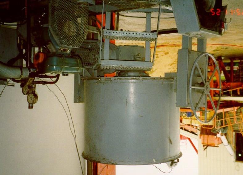
85 CEMAGREF-IMG A - 75

86 IBB A - 76

87 Two-point test A - 77

88 Batch plant Transportation of concrete to the rheometers A - 78

89 Appendix B: Pictures from the slump tests The slump tests, depicted here, were carried out at the same time as the concrete was being tested in the rheometers. Mixture #1 Mixture #2 A - 79

90 Mixture #3 Mixture #4 A - 8

91 Mixture #5 Mixture #6 A - 81

92 Mixture #7 Mixture #8 A - 82

93 Mixture #9 Mixture #1 A - 83

94 Mixture #11 Mixture #12 A - 84

95 Appendix C: Data from the rheometers Data and graphs from the BML All the mixes were run twice and are shown here and in the graphs, but only the first run was used in the report to compare with the other rheometers. Velocity Mix-1 Mix-2 Mix-3 Mix-4 Mix-5 Mix-6 Mix-7 Mix-8 Mix-9 Mix-1 Mix-11 Mix-12 (rev/s) (Nm) (Nm) (Nm) (Nm) (Nm) (Nm) (Nm) (Nm) (Nm) (Nm) (Nm) (Nm),46 21,92 No 2,84 No 14,18 No 19,1 No 24,83 No 6,85 No 5, No 12,82 No 3,51 No 8,19 No 9,8 No 12,93 No,4 2,17 No 2,64 No 12,87 No 17,66 No 21,2 No 6,35 No 4,25 No 11,98 No 3,23 No 7,43 No 9,59 No 12,22 No,34 19,11 No 2,34 No 11,98 No 16,66 No 2,23 No 5,42 No 3,73 No 11,8 No 3,1 No 7,1 No 8,98 No 11,64 No,28 16,92 No 2,9 No 1,78 No 15,64 No 18,45 No 4,84 No 3,32 No 11,32 No 2,83 No 6,16 No 8,41 No 11,14 No,21 15,23 No 1,86 No 9,38 No 14,92 No 18,19 No 4,25 No 3,5 No 11,7 No 2,6 No 5,75 No 8,13 No 1,55 No,15 13,99 No 1,63 No 8,34 No 13,71 No 15,8 No 3,59 No 2,44 No 1,62 No 2,34 No 5,26 No 7,87 Yes 1,1 No,9 13,13 Yes 1,43 Yes 7,69 Yes 14,3 Yes 14,64 No 3,7 Yes 1,95 No 1,11 No 2,12 No 4,66 No 7,69 Yes 9,18 No,3 17,1 2, 1,6 15,1 18,6 5, 3,4 11,6 2,7 6,4 8,2 11,6 Velocity Mix-1B Mix-2B Mix-3B Mix-4B Mix-5B Mix-6B Mix-7B Mix-8B Mix-9B Mix-1B Mix-11B Mix-12B (rev/s) (Nm) (Nm) (Nm) (Nm) (Nm) (Nm) (Nm) (Nm) (Nm) (Nm) (Nm) (Nm),46 2,79 No 13,46 No 16,97 No No 7,33 No 5,13 No 13,28 No 3,54 No 8,38 No 11,8 No 14,2 No,4 2,45 No 12,1 No 15,69 No No 6,45 No 4,54 No 12,74 No 3,17 No 7,49 No 1,26 No 13,63 No,34 2,19 No 11,63 No 15,2 No No 5,47 No 3,96 No 11,68 No 2,94 No 6,76 No 9,62 No 13,13 No,28 1,97 No 1,12 No 13,66 No No 5,9 No 3,42 No 11,52 No 2,76 No 6,21 No 9,22 No 12,39 No,21 1,81 No 9,14 No 13,69 No No 4,54 No 2,9 No 11,17 No 2,47 No 5,67 No 8,83 No 11,89 No,15 1,51 No 7,96 No 12,74 Yes No 3,88 No 2,63 No 1,2 No 2,34 No 4,99 No 8,77 Yes 11,14 No,9 1,4 Yes 7,25 Yes 12,51 Yes No 3,29 Yes 2,13 No 1,3 No 2,12 No 4,37 No 8,6 Yes 1,3 No,3 2, 1,2 13,5 5,2 3,5 12, 2,7 6,2 8,9 12,9 A - 85

96 Torque (Nm) Mix-1 y = 25,99x + 9,92 R 2 =,99 Mix-1 Control Torque (Nm) Mix-2 y = 3,95x + 1,2 R 2 = 1, Mix-2 Control Mix-2B Control Torque (Nm) Mix-3 y = 18,77x + 5,5 R 2 = 1, Mix-3 Control Mix-3B Control,25,5 Velocity (rev/s),25,5 Velocity (rev/s),25,5 Velocity (rev/s) Torque (Nm) Mix-4 y = 16,37x + 11,25 Mix-4 R 2 =,99 Control Mix-4B Control Torque (Nm) Mix-5 y = 25,3x + 11,99 R 2 =,92 Mix-5 Control Torque (Nm) Mix-6 y = 1,62x + 1,96 Mix-6 Control R 2 =,99 Mix-6B Control,25,5 Velocity (rev/s),25,5 Velocity (rev/s),25,5 Velocity (rev/s) 25 Mix-7 25 Mix-8 25 Mix-9 Torque (Nm) Mix-7 y = 7,71x + 1,26 R 2 =,98 Control Mix-7B Control Torque (Nm) Mix-8 y = 6,64x + 9,56 R 2 =,97 Control Mix-8B Control Torque (Nm) Mix-9 y = 3,65x + 1,8 R 2 = 1, Control Mix-9B Control,25,5 Velocity (rev/s),25,5 Velocity (rev/s),25,5 Velocity (rev/s) 25 Mix-1 25 Mix Mix-12 Torque (Nm) Mix-1 y = 9,3x + 3,79 R 2 =,99 Control Mix-1B Control Torque (Nm) Mix-11 y = 7,28x + 6,52 R 2 =,97 Control Mix-11B Control Torque (Nm) Mix-12 y = 9,63x + 8,44 R 2 =,99 Control Mix-12B Control,25,5 Velocity (rev/s),25,5 Velocity (rev/s),25,5 Velocity (rev/s) A - 86

97 The following table gives the summary of the calculated results. Mix Test G-value H-value r dg dh Seg. Yield Pl. Visc Time Date Time no. no. (Nm) (Nm s) (Nm) (Nm s) (Pa) (Pa s) (min) (dd/mm/yy) (hh/mm/ss) 1 1 9,81 25,93,997,28, , /1/2 1:17:26 2 1,13 21,21,991,37, , /1/2 1:3: ,1 3,95,999,6, ,4 1 24/1/2 12:4:21 2,9 3,91,995,14, ,2 1 24/1/2 12:13: ,42 18,72,999,16, ,4 1 24/1/2 14:51:54 2 5,36 17,22,994,33, ,8 1 24/1/2 14:59: ,17 16,36,997,22, , 1 24/1/2 16:55:39 2 1,3 13,74,968,81, ,5 1 24/1/2 17:3: ,11 24,64,974,7, ,4 1 25/1/2 9:56:18 2 Error 45,11 33,13,956 1,7 1, ,8 1 25/1/2 1:3:11 6-SCC 1 1,91 1,61,997,16, , 1 25/1/2 12:1:45 2 2,13 1,69,99,33, ,4 1 25/1/2 12:18:3 3 Thixotrop 2,19 14,58,997,19, ,4 4 25/1/2 12:21: ,24 7,69,994,19, ,7 1 25/1/2 15:13:22 2 1,31 7,93,996,16, ,9 1 25/1/2 15:18:43 3 Thixo 1,3 1,34,998,13, ,2 4 25/1/2 15:26:2 4 Thixo 1,43 9,77,998,11, ,7 4 25/1/2 15:29: ,53 6,62,989,23, ,1 1 25/1/2 18:2:19 2 9,5 8,79,983,33, ,7 1 25/1/2 18:9: ,79 3,64,999,5, , 1 36 min 26/1/2 9:53:42 2 1,74 3,65,993,13, , 1 min 26/1/2 9:59:48 3 Thixotrop 1,81 3,83,995,11, ,6 4 min 26/1/2 1:6: ,75 9,27,997,15, ,9 1 26/1/2 11:4:45 2 3,36 1,38,997,15, ,9 1 26/1/2 11:47:38 3 Thixo 3,69 1,62,996,18, , 4 26/1/2 11:51: ,5 7,24,989,34, ,9 1 26/1/2 15:11:2 2 6,77 8,86,986,42, , 1 26/1/2 15:17: ,41 9,59,998,12, , 1 27/1/2 1:14:2 2 9,51 1,24,997,16, ,1 1 27/1/2 1:22: ,84 13,28,996,19, ,4 1 27/1/2 1:49:33 Oil error 1 plug 7,74 1,74,995,2, ,9 1 27/1/2 11:31:5 A - 87

98 The thixotropy was evaluated for four mixtures; Mixture #6, Mixture #7, Mixture #9 and Mixture #1. Mixture #7 was tested twice (Na-7A and Na-7B) with almost identical results. The thixotropic properties were evaluated by determining up and down curves (up and down refer to the increase or decrease of the velocity). The area between the up and down curves is the rate of work per unit volume ; it cannot be directly characterized as a material parameter as it depends heavily on the shear history of the material tested. The size of the thixotropy area should also be related to the yield value of the material. The thixotropy is lower for mixture #9 though relative to the yield value for mixture #1 is the lowest. The thixotropy is significantly higher for mixture # Thixotropy Mix-6 Mix-7A Mix-7B Mix-9 Mix-1 N m 4 2,2,4 V e lo c ity ( r e v /s ) A - 88

99 Data and graphs obtained using the BTRHEOM The dotted line represents the modified Bingham model fitted to the points. 1 Mix 1 1 Mix torque (N.m) 6 4 torque (N.m) rotation speed (rev/s) rotation speed (rev/s) 2 Mix 2 1 Mix torque (N.m) 1 torque (N.m) rotation speed (rev/s) rotation speed (rev/s) 6 Mix 3 4 Mix 6 3 torque (N.m) 4 2 torque (N.m) rotation speed (rev/s) rotation speed (rev/s) A - 89

100 4 Mix 7 4 Mix torque (N.m) 2 torque (N.m) rotation speed (rev/s) rotation speed (rev/s) 8 Mix 8 5 Mix torque (N.m) 4 torque (N.m) rotation speed (rev/s) rotation speed (rev/s) 3 Mix 9 1 Mix 12 8 torque (N.m) 2 1 torque (N.m) first measurement first, fitted 3 minutes later second, fitted rotation speed (rev/s) rotation speed (rev/s) A - 9

101 The following tables show the data points used for the graph above. The readings were recorded by decreasing rotation speed. The concrete was vibrated prior to start of the measurements to ensure good filling of the bucket, unless stated otherwise. Mixture #1 Point Speed Torque n (rev/s) (N m) Mixture #2: The concrete was not vibrated prior to measurement. Point Speed Torque n (rev/s) (N m) Mixture #3. Point Speed Torque n (rev/s) (N m) Mixture #4 Point Speed Torque n (rev/s) (N m) Mixture #5 Point Speed Torque n (rev/s) (N m) Mixture #6: The concrete was not vibrated prior to measurement. Point Speed Torque n (rev/s) (N m) A - 91

102 Mixture #7: The concrete was not vibrated prior to measurement. Point Speed Torque n (rev/s) (N m) Mixture #8 Point Speed Torque n (rev/s) (N m) Mixture 9. The concrete was not vibrated prior to measurement. Point Speed Torque n (rev/s) (N m) Mixture 1 Point Speed Torque n (rev/s) (N m) Mixture #11 Point Speed Torque n (rev/s) (N m) Mixture #12 Point Speed Torque n (rev/s) (N m) A - 92

103 Mixture #12: Second measurement (3 min after the first one) Point Speed Torque n (rev/s) (N m) Concrete parameters calculated from the down curves Date Mixture File Yield stress (Pa) Plastic viscosity (Pa s) 1/24/ 1 LNAC /24/ 2 LNAC /24/ 3 LNAC /24/ 4 LNAC /25/ 5 LNAC9B /25/ 6 LNAC /25/ 7 LNAC /25/ 8 LNAC /26/ 9 LNAC /26/ 1 LNAC /26/ 11 LNAC See note 1/26/ 12 LNAC Note for Mixture #11: the lowest rotation speed was recorded as, leading to an error in the data processing. These values were calculated later, from the raw data, with the same equations, without the point at speed zero. A - 93

104 Data and graphs obtained using the CEMAGREF-IMG List of the various tests and comments. Mixture # Text file for the Text file for the seal concrete Height of the sheared concrete sample (m) Comments 1 Mix1a.txt Seal1a.txt Mix2a.txt Seal2a.txt.678 Segregation at the end of the test: width 7 mm, depth of segregation 3 mm to 7 mm 3 Mix3a.txt Seal3a.txt.67 4 Mix4b.txt Seal4a.txt Mix5b.txt Seal5a.txt.345 Concrete too stiff to start the test. Part of the concrete is removed from the rheometer. Test restarted at T+33 min 6 Mix6a.txt Seal6a.txt Mix7a.txt Seal7a.txt.635 Light segregation at the end of the test: width=6 mm, depth: 1 mm 8 Mix8a.txt Seal8a.txt Mix9a.txt Seal9a.txt.65 1 Mix1a.txt Seal1a.txt Mix11a.txt Seal11a.txt Mix12a.txt Seal12a.txt.645 A second test is performed at To+43 min. corresponding to Mix12b.txt and Seal12a.txt. For this test, vibration is needed to re-start the rotation, applied with vibrating poker put in the concrete specimen. The measurements of the width of the sheared zone are given in Appendix C. Direct calculation of the shear yield stress C C R We have τ = 2 so 3 c τ = R c and finally: τ = 2τ 2πhR c πhr c R c The mean error on the measurement of the width of the sheared zone is estimated to be equal to the maximum diameter of the aggregate (i.e., 1.25 time diameter 16 mm for mixture #1 to #7, 1.25 time diameter 2 mm for mixture #8 to #11 and 1.25 time diameter 6.3 mm for mixture #12) The following figures present the values of the shear yield stress calculated for each mixture and for each rotation speed, with their corresponding error bar. In a perfect experiment, all the values of calculated shear yield stress should be equal on each figure. This was not the case so, for each mixture, the shear yield stress was calculated as the mean of the lowest value of the tops of the error bars and the largest value of the bottoms of the error bars. This shear yield stress is considered to be acceptable only if it is included in all error bars. According to this procedure, we can see on the following figures, that the values obtained for mixture #3, mixture #9 and mixture #12 (respectively: 85 Pa, 423 Pa and 1148 Pa) are not acceptable. The decrease of the calculated shear yield stress values with the rotation speed observed with mixture #3 is probably due to the horizontal segregation of coarse aggregate, which tends to occur more and more during the test, because of the increase of the dead zone. Then, the mixture-composition is assumed to change, from the inner cylinder vicinity (where the A - 94

105 mixture is richer in fine elements) to the outer cylinder (where the mixture is leaner). The tendency observed for mixture #9 and mixture #12 is not clear, and it could be due to an error in the measurements. No measurement was available for mixture #5, owing to the fact that the concrete top surface was hardly visible, and for the second test with mixture #12. Only one measurement was available for each of Mixture #1 and #4. The sheared zone width observed on mixture #4 was low, as compared to the maximum diameter of aggregate, even at the maximum rotation speed. Therefore, it can be assumed that the part of the sample that was sheared during the test was more a mortar than the concrete in bulk. Finally, the shear yield stress calculated is not an exact value but a minimum bound of the concrete yield stress. Yield values deduced from the width of the sheared zone and the equation 21 in Section 3.3 (main part of this report). Mixtur e # t (Pa) > * - *second test A - 95

106 Width of the sheared zone E c Mixture 1 W (rad/s) Experimental Ec (mm) Mixture 2 W (rad/s) Experimental Ec (mm).9 5 Mixture 3 W (rad/s) Mixture 4 W (rad/s) Mixture 6 W (rad/s) Experimental Ec (mm) Experimental Ec (mm) Experimental Ec (mm) Mixture 7 W (rad/s) Mixture 8 W (rad/s) Mixture 9 W (rad/s) Experimental Ec (mm) Experimental Ec (mm) Experimental Ec (mm) A - 96

107 Mixture 1 W (rad/s) Mixture 11 W (rad/s) Mixture 12 W (rad/s) Experimental Ec (mm) Experimental Ec (mm) Experimental Ec (mm) A - 97

108 Values of the shear yield stress calculated with Equation 21 from Section 3.3 for different rotation speeds. The horizontal dotted lines give the value adopted for each mixture. To be acceptable a dotted line must pass through the error bars. 25 Mix #1 14 Mix #3 (Pa) (Pa) W (rad/s) W (rad/s) 6 Mix #2 25 Mix #4 5 2 (Pa) (Pa) W (rad/s) W (rad/s) A - 98

109 (P Mix# W (rad/s) Mix #7 (Pa) Mix # W (rad/s) Mix # (Pa) 3 2 (Pa) W (rad/s) W (rad/s) 2 Mix #8 14 Mix #12 (Pa) 15 1 (Pa) W (rad/s) W (rad/s) 6 Mix #9 5 (Pa) W (rad/s) A - 99

110 Fitting of the curves for torque vs. rotation speed obtained for the seals The following table summarizes the data concerning the fitting of the experimental curves obtained for the seals alone. Figures of these curves can be found below. Curve fitting for measurements on the seal alone Mixture Equation Mean error Range of fit # (N m) W max (rad/s) W min (rad/s) 1 C seal = Ω C seal = Ω C seal = Ω C seal = Ω C seal = Ω C seal = Ω C seal = Ω C seal = Ω C seal = Ω C seal = Ω C seal = Ω C seal = Ω * C seal = Ω *second test Analysis with the Bingham model The results are summarized in the table below. Figures of these curves can be found below under Experimental and fitted torque-rotation speed curves. It can be seen that, for some mixtures, the τ values calculated with the Bingham model are significantly different from the values calculated directly. This means that even if the inner cylinder of the CEMAGREF-IMG rheometer is equipped with a metallic grid, a significant slippage occurs between the cylinder and some concretes. This phenomenon may be related to a horizontal segregation, where coarse particles are expelled from the sheared zone, so that shear tends to be concentrated in a thin annulus around the rotating cylinder, where the material is more fluid than in the rest of the sample. A - 1

111 Results according the Bingham model Mixture # t (Pa) µ (Pa s) Mean error g& max Range of fit (N m) (1/s) W max (rad/s) W min (rad/s) * *second test Summary The table below summarizes the values of τ calculated with the Bingham model and from the width of the sheared zone E c. When the difference is high, slippage has probably occurred between the inner cylinder and the concrete sample. In this case, the rheological parameters calculated with the Bingham model are not valid and should not be considered. The figure on page A-12 shows the differences observed between the two methods as a function of the slump. It appears that for slump lower than approximately 11 mm, slippage occurs, as in mixture #5 and 12. Again in this case, the rheological parameters evaluated with Bingham model are not valid and cannot be used for these tests. According to Direct calculation of the shear yield stress (page A-94), mixture #3 was certainly subject to segregation and rheological parameters are probably not relevant. Mixture #9 and #12 (for the first test) were probably not subject to slippage because their slumps were respectively 232 mm and 15 mm; moreover, the shear yield stress calculated with the Bingham model is close to the one calculated with E c. Therefore, even if the direct measurement of the shear yield stress was subject to errors in measurement, the rheological values calculated with Bingham can be accepted. A - 11

112 Comparisons of shear yield stresses calculated directly from E c and with the Bingham model assuming no slippage Mixture t calculated with t calculated from Difference (Pa) Slump (cm) # Bingham (Pa) E c (Pa) >2138 > * * second test Observed difference (Pa) Slump (cm) Difference between the shear yield stress calculated with Equation 21 or Equation 28 (see Section 3.3) and the slump Finally, the only reliable rheological values for use in comparing the different rheometers are summarized in the table below. A - 12

113 Rheological values judged to be reliable Mixture t calculated with t calculated with µ calculated with # E c (Pa) Bingham (Pa ) Bingham (Pa s) > * * second test For further investigations with the CEMAGREF-IMG rheometer, it is proposed to fix blades on the surface of the inner cylinder to avoid slippage. A - 13

114 Experimental and fitted torque-rotation speed curves C seal: torque applied to the seal alone Net torque: is torque really applied to the concrete sample MIXTURE Torque Cseal (Nm) Seal1a.txt Rotation speed (rad/s) Net torque C (Nm) Mix1a.txt Rotation speed (rad/s) Legend + Experimental values - Curve fitting (see Equation 28 and equation 29 in Section 3.3) A - 14

115 MIXTURE Torque Cseal (Nm) Seal 2a.txt Rotation speed (rad/s) 4 35 Net torque C (Nm) Mix2a.txt Rotation speed (rad/s) Legend + Experimental values - Curve fitting (see Equation 28 and equation 29 in Section 3.3). A - 15

116 MIXTURE Torque Cseal (Nm) Seal 3a.txt Rotation speed (rad/s) 11 1 Net torque C (Nm) Mix3a.txt Rotation speed (rad/s) Legend + Experimental values - Curve fitting (see Equation 28 and equation 29 in Section 3.3). A - 16

117 MIXTURE Torque Cseal (Nm) Seal4a.txt Rotation speed (rad/s) Net torque C (Nm) Mix4b.txt Rotation speed (rad/s) Legend + Experimental values - Curve fitting (see Equation 28 and equation 29 in Section 3.3). A - 17

118 MIXTURE Torque Cseal (Nm) Seal5a.txt Rotation speed (rad/s) 8 7 Net torque C (Nm) Mix5b.txt Rotation speed (rad/s) Legend + Experimental values - Curve fitting (see Equation 28 and equation 29 in Section 3.3). A - 18

119 MIXTURE Torque Cseal (Nm) Seal6a.txt Rotation speed (rad/s) 7 6 Net torque C (Nm) Mix6a.txt Rotation speed (rad/s) Legend + Experimental values - Curve fitting (see Equation 28 and equation 29 in Section 3.3). A - 19

120 MIXTURE Torque Cseal (Nm) Seal7a.txt Rotation speed (rad/s) 6 5 Net torque C (Nm) Mix7a.txt Rotation speed (rad/s) Legend + Experimental values - Curve (see Equation 28 and equation 29 in Section 3.3). A - 11

121 MIXTURE Torque Cseal (Nm) Seal8a.txt Rotation speed (rad/s) Net torque C (Nm) Mix8a.txt Rotation speed (rad/s) Legend + Experimental values - Curve fitting (see Equation 28 and equation 29 in Section 3.3). A - 111

122 MIXTURE Torque Cseal (Nm) Seal9a.txt Rotation speed (rad/s) 4 35 Net torque C (Nm) Mix9a.txt Rotation speed (rad/s) Legend + Experimental values - Curve fitting (see Equation 28 and equation 29 in Section 3.3). A - 112

123 MIXTURE Torque Cseal (Nm) Seal1a.txt Rotation speed (rad/s) 7 6 Net torque C (Nm) Mix1a.txt Rotation speed (rad/s) Legend + Experimental values - Curve fitting (see Equation 28 and equation 29 in Section 3.3). A - 113

124 MIXTURE Torque Cseal (Nm) Seal11a.txt Rotation speed (rad/s) 9 8 Net torque C (Nm) Mix11a.txt Rotation speed (rad/s) Legend + Experimental values - Curve fitting (see Equation 28 and equation 29 in Section 3.3). A - 114

125 MIXTURE Torque Cseal (Nm) Seal12a.txt Rotation speed (rad/s) 11 1 Net torque C (Nm) Mix12a.txt Rotation speed (rad/s) Legend + Experimental values - Curve fitting (see Equation 28 and equation 29 in Section 3.3). MIXTURE 12 (second test) A - 115

126 18 16 Torque Cseal (Nm) Seal12a.txt Rotation speed (rad/s) Net torque C (Nm) Mix12b.txt Rotation speed (rad/s) Legend + Experimental values - Curve fitting (see Equation 28 and equation 29 in Section 3.3). A - 116

127 Data and graphs obtained using the IBB The dotted line represents the modified Bingham model fitted to the points. Mix 1 Mix 5 1,8 y =,68x -,736 R 2 =,96 1,8 y =,68x -,268 R 2 =,898 Speed (rev/s),6,4 Speed (rev/s),6,4,2, Torque (Nm) Torque (Nm) Mix 2 Mix 6 Speed (rev/s) 1,8,6,4 y =,187x -,64 R 2 =,967 Speed (rev/s) 1,8,6,4 y =,97x -,174 R 2 =,961,2, Torque (Nm) Torque (Nm) Mix 3 Mix 7 1 1,8 y =,76x -,277 R 2 =,986,8 y =,17x -,92 R 2 =,955 Speed (rev/s),6,4 Speed (rev/s),6,4,2, Torque (Nm) Torque (Nm) Mix 4 Mix 8 1 1,8 y =,86x -,638 R 2 =,941,8 y =,113x -,645 Speed (rev/s),6,4 Speed (rev/s),6,4 R 2 =,973,2, Torque (Nm) Torque (Nm) A - 117

128 Mix 9 Mix Speed (rev/s),8,6,4 y =,165x -,156 R 2 =,978 Speed (rev/s),8,6,4 y =,11x -,688 R 2 =,981,2, Torque (Nm) Torque (Nm) Mix 1 Mix 12b 1 1 Speed (rev/s),8,6,4 y =,113x -,223 R 2 =,967 Speed (rev/s),8,6,4 y =,81x -,651 R 2 =,935,2, Torque (Nm) Torque (Nm) Mix 11 1 Speed (rev/s),8,6,4 y =,152x -,63 R 2 =,896, Torque (Nm) A - 118

129 The following tables show the data points used for the graphs above. The readings were recorded by decreasing rotation speed. The data used for calculations are from Point 1 (Point is excluded) to Point 6 included. The speeds equal to are not taken into account for calculations. For each mixture the following parameters were used: H = Yield stress; G = Viscosity; R2 = correlation factor; M and B are parameters to calculate the yield stress and viscosity Mixture #1: Parameters values are: H = ; G = 1.842; R2 =.96; M =.68; B = Point # Torque N m Speed Rev/s Mixture #2: Parameters values are: H = 5.345; G =.341; R2 =.966; M =.187; B = -.64 Point # Torque N m Speed Rev/s Mixture #3: Parameters values are: H = 13.27; G = 3.669; R2 =.986; M =.76; B = Point # Torque N m Speed Rev/s Mixture #4: Parameters values are: H = ; G = 7.438; R2 =.941; M =.86; B = Point # Torque N m Speed Rev/s A - 119

130 Mixture #5: Parameters values are: H = ; G = 3.915; R2 =.898; M =.68; B = Point # Torque N m Speed Rev/s Mixture #6: Parameters values are: H = 1.314; G = 1.8; R2 =.961; M =.97; B = Point # Torque N m Speed Rev/s Mixture #7: Parameters values are: H = 9.311; G =.856; R2 =.955; M =.17; B = -.92 Point # Torque N m Speed Rev/s Mixture #8: Parameters values are: H = 8.846; G = 5.71; R2 =.973; M =.113; B = Point # Torque N m Speed Rev/s Mixture #9: Parameters values are: H = 6.62; G =.948; R2 =.978; M =.165; B = Point # Torque N m Speed Rev/s Mixture #1: Parameters values are: H = 8.883; G = 1.982; R2 =.967; M =.113; B = Point # Torque N m Speed Rev/s A - 12

131 Mixture #11: Parameters values are: H = 6.568; G = 3.959; R2 =.896; M =.152; B = -.63 Point # Torque N m Speed Rev/s Mixture #12: Parameters values are: H = 9.74; G = 6.237; R2 =.98; M =.11; B = Point # Torque N m Speed Rev/s Mixture #12b: Parameters values are: H = ; G = 8.49; R2 =.935; M =.81; B = Point # Torque N m Speed Rev/s Summary of the values calculated from the measurement with the IBB Mixture # Plastic Viscosity Yield stress Nms Nm A - 121

132 Data and graphs obtained using the Two-Point test Details of the analysis are included in Section 3.5 of the main part of this report. Mix 1 Mix 2 oil pressure (volts) concrete idling (before) idling (after) oil pressure (volts) concrete idling (before) idling (after) speed (volts) speed (volts) Mix 3 Mix 4.6 concrete.6 concrete oil pressure (volts) idling (before) idling (after) oil pressure (volts) idling (before) idling (after) speed (volts) speed (volts) Mix 5 Mix 6 oil pressure (volts) concrete idling (before) idling (after) oil pressure (volts) concrete idling (before) idling (after) speed (volts) speed (volts) A - 122

133 Mix 7 Mix 8 oil pressure (volts) concrete idling (before) idling (after) oil pressure (volts) concrete idling (before) idling (after) speed (volts) speed (volts) Mix 9 Mix concrete idling (before) idling (after).5.4 concrete idling (before) idling (after) oil p sped(volts) Mix 11.6 concrete oil pressure (volts).5 idling (before) idling (after) sped(volts).2 oil p sped(volts) Mix 12.6 concrete.5 idling (before).4 idling (after).3.2 oil presure(volts) sped(volts) A - 123

134 Summary of the results calculated from the figures above. Details of the calculations are given in Section 3.5 of the main part of this report. test number regression analysis output: oil pressure vs speed (voltages) idling concrete (after correction) intercept slope R 2 intercept slope R 2 g (Nm) h (Nms) Bingham constants yield stress (Pa) plastic viscosity (Pa.s) Notes: Mixture 4 - plastic viscosity not measurable due to low slump, yield value should be treated with caution Mixtures 3, 5, 6 - idling data from single test only (others mean of two tests) A - 124

135 Appendix D: Calibration report for the CEMAGREF-IMG Acquisition system calibration A - 125

136 Speed-meter calibration A - 126

137 A - 127

138 A - 128

139 Torque cells calibration A - 129

140 Calibration des capteur de couple du rhéomètre CEMAGREF Constat métrologique n Capteur 1 Capteur 1 C(Nm) Tension (V) C(Nm) V Couple (Nm) Couple (Nm) Capteur y = x Tension (V) Capteur y = 1.2x Tension (V) A - 13

141 Appendix E: Calculation of the Kendall coefficient of concordance Outline of the procedure for calculating Kendall s coefficient of concordance, W (summarized from Ref. [1]). n objects have been ordered according to p criteria : Criterion Object 1 2 n 1 r 11 r 21 r n1 2 r 12 r 22 r n2 p r 1p r 2p r np sum r 1. r 2. r n. r.. r ij is the rank of an object i according to criterion (apparatus) j. In our case, the objects are the mixtures and the criteria the rheometers. For each line of the table, the sum of the terms is n (n + 1) n( n +1). Then r = p 2 ij 2. If all the rankings are identical, all the terms in a given column are equal, and the r i. are equal to p, 2p, 3p. The following parameter is used : = n rij 2 S ( ri. ). If all the rankings are identical, S is i= 1 n 2 3 p (n n) 12S maximum, and S = Smax =. Kendall s W parameter is W 12 = 2 3 p (n n), and W 1. The hypothesis tested here is that the p rankings are independent. The critical value of W (at 95% confidence level) are given in a reference table (not given here) for different n and p. If the calculated value of W is higher than the reference value, the hypothesis is rejected, i.e., the rankings are not independent. A - 131

142 A - 132

143 Appendix F: Artifacts in Rheological Measurements This appendix deals with some problems related to the granular nature of fresh concrete. They are not addressed in classical fluid rheology, and they may aid in interpretation of rheometric measurements dealing with concrete. Size of tested specimen Concrete is a heterogeneous material. For making significant measurements of any of its material properties, it is essential: - to minimize the risk of spatial segregation; This has been done in the present program by designing mixtures with continuous grading size and sufficient fine particle proportions, and by taking precautions such as careful transport and re-mixing before sampling. The absence of segregation has been checked by a number of fresh concrete analyses (see Chapter 2); - to test specimens, the sizes of which are large compared to the largest dimension of heterogeneity. Here, this dimension is taken as the maximum size of aggregate (MSA). Assuming that a ratio of 1 between test specimen and MSA is acceptable, and taking a MSA of 2 mm, this would lead to a cube having a 2 mm length, which makes a volume of 8 L. However, there is not any clear threshold in this respect: the bigger the specimen, the closer the measurement is to the real value. On the contrary, the smaller the specimen, the lower the correlation between the apparent and real properties. Let us also note that it is the volume of sheared concrete that matters, not the total volume of concrete contained in the apparatus. Slip at the boundaries of the specimen All methods used to deduce basic rheological parameters from bulk measurements in rheometers implicitly assume that the velocity gradient in the tested specimen is continuous up to the interface. This means that the velocity between two parallel, plane surfaces is supposed to vary linearly with distance between the surfaces. This assumption is correct for a Newtonian liquid like some oil and water, at least for low Reynolds numbers. Figure F-1: Velocity gradient in a sheared layer. A) without slip; B) with slip, at low rate; C) with slip, at high rate. A - 133

144 However, with granular suspensions like fresh concrete, a interfacial layer forms spontaneously in the vicinity of the wall, owing to the exclusion of coarse particles, which makes the material locally more fluid than the bulk of the suspension. From a macroscopic viewpoint, everything happens as if the strain rate was concentrated in this limit layer, creating a sliding motion. This phenomenon is well known in concrete pumping technology [2]. Various authors [2, 3, 4, 5] have proposed the following model to describe this phenomenon: τ τ + η. = (F- 1 ), i v g where τ is the shear stress, τ,i is the interfacial yield stress, η is the interfacial viscous constant and v g the sliding velocity. Of course, τ,i is always smaller than the concrete yield stress τ. This means that when a shear force is applied to the material by the wall, there is first a sliding motion (with no shear in the bulk of the concrete specimen). Concrete starts to shear only when the shear stress τ attains the yield stress, which means that the sliding velocity is high enough (see Figure F-1). Applying this concept to the basic rheometric problem, let us assume that an ideal Couette coaxial viscometer is used, with e being the gap between the cylinders, and R the mean radius and the ratio e/r << 1. With a conventional Bingham material, and no slip at the interface, the analysis of the test is performed as follows: τ = τ + µ γ& (F- 2 ) Ω R = e γ& (F- 3 ) Γ = 2π R 2 h τ (F- 4 ) Γ 2π R 2 h = τ + µ R e Ω (F- 5 ) where - Γ is the torque (in N m); - h is the height of the specimen (in m); - µ is the concrete plastic viscosity (in Pa s); and - Ω the relative angular speed (in rad/s)between the two cylinders. A - 134

145 To deduce the basic parameters τ and µ from the macroscopic measurements, the Γ R strategy is to plot the ratio as a function of Ω, then to identify the yield 2πR 2 h e stress with the intercept and the plastic viscosity with the slope of the obtained straight line. Now, let suppose that a slip, described by Equation F-1, to take place at the exterior interface. When the slip velocity is high enough, the relationship between the torque and the angular speed is still linear, and we have: Ω R v = e g γ& (F- 6 ) Ω R v τ + e g = τ + µ = τ, i ηvg (F- 7 ) which gives finally, when the concrete specimen is sheared: Γ 2π R 2 = τ h ap. ap. + µ R e Ω ( F-8 ) where τ ap. η µ / e = τ + τ, i is the apparent yield stress, and µ / e + η µ / e + η µ ap. η = µ µ / e + η is the apparent plastic viscosity. To assess the significance of this artifact, we will refer to the thesis of Kaplan [2], who measured the four needed parameters τ, µ, τ,i and η for a variety of 37 mixtures. Taking arbitrarily a value of 1 mm for e, mean values of.47 and.39 are found for the ratios τ ap. /τ and µ ap. /µ, respectively. It means that for a coaxial viscometer having a mean distance of 1 mm between inner and outer cylinder, and no roughness to avoid slippage on the external wall, an error of more than 5 % can occur in the experimental assessment of Bingham parameters. A - 135

146 Ω R v g Ω R Figure F-2: Rate field in the gap of the viscometer. A) with no slip; B) with slip at the outer wall. Wall effect In a dry packing of particles, it is well known that the porosity tends to increase when the distance between walls decreases. This is due to the supplementary porosity appearing at the interface between grains and walls. Since the wall has no curvature, the volume of individual voids is greater when a border surface of these voids is constituted by the wall of the container (see Figure F-3). In other words, the porosity is higher near a wall. V p v d d/2 Figure F-3: Wall effect in a dry packing of particles. In the perturbed interfacial volume V p, porosity is higher than in the bulk of the specimen [6]. Such an effect also takes place in granular suspensions. During the research devoted to self-compacting concrete rheometry [7], tests were carried out where the height of the sheared specimen was changed (see Figure F-4). In this set-up, a supplementary blade system was added to the original ones, the height of which could be adjusted. A - 136

147 upperblade supplementary upperblade rotating part fixed bowl sheared zone lower blade rheometer axis Figure F-4: Modification of BTRHEOM rheometer, to display wall effect in rheometric measurements. A grid was fixed on the top of intermediate blades (see Figure F-5) and a piece of plastic was added to fill the space under the bottom blades to limit the dead zones to the interstices of the blades. So the tests could be considered as confined tests. In the first series of tests, confined tests were performed on mixtures having a maximum aggregate size of 16 mm. The effect of interblade distance and coarse/fine aggregate ratio (G/S) on the apparent Bingham constants was investigated. Test results are displayed in Figure F-6. It can be seen that strong perturbations take place as soon as the ratio between interblade distance and maximum size of aggregate is less than four. As a general trend, apparent rheological parameters tend to increase with the wall effect. This could be anticipated, since the porosity of the mixture tends to grow, while the water dosage remains constant. The higher the aggregate content in the mixture, the more pronounced the wall effect. A - 137

148 Figure F-5: Confining grid. A door can be seen on the south-west part of the wheel, through which concrete could be poured into the test zone [6]. 25 G/S=,75 12 G/S=,75 Shear yield stress (Pa) G/S=1 G/S=1,3 G/S=1,5 Plastic viscosity (Pa s) G/S=1 G/S=1,3 G/S=1, Inter-blade distance/dmax ratio Inter-blade distance/dmax ratio Figure F-6: Confined tests performed on a series of mixtures, with various interblade distances and coarse/fine aggregate ratios [6]. In a second series [7] of confined tests, a self-compacting mixture with a maximum size of 12.5 mm was tested in this set-up. The yield stress still tended to increase while the plastic viscosity decreased with the wall effect (see Figure F-7). This could be attributed to the ease of accumulation of coarse aggregates in the voids of the blades (since the mixture was not originally saturated in coarse aggregate). A - 138