Linear Programming. Xi Chen. Department of Management Science and Engineering International Business School Beijing Foreign Studies University

Transcription

1 Linear Programming Xi Chen Department of Management Science and Engineering International Business School Beijing Foreign Studies University Xi Chen Linear Programming 1 / 148

2 Introduction 1 Introduction 2 The Simplex Method 3 Sensitivity Analysis 4 Duality Theory Xi Chen (chenxi0109@bfsu.edu.cn) Linear Programming 2 / 148

3 Introduction Example 1 Giapetto s Woodcarving, Inc., manufactures two types of wooden toys: soldiers and trains. Demand for trains is unlimited, but at most 40 soldiers are bought each week. A soldier sells for $27 and uses $10 worth of raw materials. Each soldier that is manufactured increases Giapetto s variable labor and overhead costs by $14. A train sells for $21 and uses $9 worth of raw materials. Each train built increases Giapetto s variable labor and overhead costs by $10. The manufacture of wooden soldiers and trains requires two types of skilled labor: carpentry and finishing. A soldier requires 2 hours of finishing labor and 1 hour of carpentry labor. A train requires 1 hour of finishing and 1 hour of carpentry labor. Each week, Giapetto can obtain all the needed raw material but only 100 finishing hours and 80 carpentry hours. How to maximize Giapetto s weekly profit? Xi Chen (chenxi0109@bfsu.edu.cn) Linear Programming 3 / 148

4 Introduction Decision Variables: The decision variables completely describe the decisions to be made. Denote by x 1 the number of soldiers produced each week, and by x 2 the number of trains produced each week. Objective Function: The function to be maximized or minimized is called the objective function. Since fixed costs (such as rent and insurance) do not depend on the values of x 1 and x 2, Giapetto can concentrate on maximizing his weekly profit, i.e., Constraints: max 3x 1 + 2x 2. 1 Each week, no more than 100 hours of finishing time may be used. 2 Each week, no more than 80 hours of carpentry time may be used. 3 Because of limited demand, at most 40 soldiers should be produced each week. 2x 1 + x 2 100, x 1 + x 2 80, x Sign Restrictions: x 1 0 and x 2 0. Xi Chen (chenxi0109@bfsu.edu.cn) Linear Programming 4 / 148

5 Introduction Definition 1.1 A function f (x 1, x 2,..., x n ) of x 1, x 2,..., x n is a linear function if and only if for some set of constants c 1, c 2,..., c n, f (x 1, x 2,..., x n ) = c 1 x 1 + c 2 x c n x n. For any linear function f (x 1, x 2,..., x n ) and any number b, the inequalities f (x 1, x 2,..., x n ) b and f (x 1, x 2,..., x n ) b are linear inequalities. A linear programming problem (LP) is an optimization problem for which we do the following: 1 We attempt to maximize (or minimize) a linear function of the decision variables (objective function). 2 The values of the decision variables must satisfy a set of constraints. Each constraint must be a linear equation or linear inequality. 3 A sign restriction is associated with each variable. For any variable x i, the sign restriction specifies that x i must be either nonnegative (x i 0) or unrestricted in sign (urs). Xi Chen (chenxi0109@bfsu.edu.cn) Linear Programming 5 / 148

6 Assumptions Introduction Proportionality: The contribution of the objective function from each decision variable is proportional to the value of the decision variable, and so does each linear constraint. Additivity: The value of the objective function is the sum of the contributions from individual variables, and so does each linear constraint. Divisibility: Each decision variable be allowed to assume fractional values. A linear programming problem in which some or all of the variables must be nonnegative integers is called an integer programming problem. Certainty: Each parameter (objective function coefficient, righthand side, and technological coefficient) is known with certainty. Xi Chen (chenxi0109@bfsu.edu.cn) Linear Programming 6 / 148

7 Introduction Definition 1.2 The feasible region for an LP is the set of all points that satisfies all the LP s constraints and sign restrictions. Any point that is not in an LP s feasible region is said to be an infeasible point. Definition 1.3 For a maximization problem, an optimal solution to an LP is a point in the feasible region with the largest objective function value. Similarly, for a minimization problem, an optimal solution is a point in the feasible region with the smallest objective function value. Most LPs have only one optimal solution. Some LPs have no optimal solution. Some LPs have an infinite number of solutions. Xi Chen (chenxi0109@bfsu.edu.cn) Linear Programming 7 / 148

8 Introduction The Graphical Solution Xi Chen Linear Programming 8 / 148

9 Introduction Definition 1.4 A constraint is binding if the left-hand side and the right-hand side of the constraint are equal when the optimal values of the decision variables are substituted into the constraint. If they are unequal with respect to the optimal solutions, a constraint is nonbinding. Definition 1.5 A set of points S is a convex set if the line segment joining any pair of points in S is wholly contained in S. For any convex set S, a point P in S is an extreme point if each line segment that lies completely in S and contains the point P has P as an endpoint of the line segment. Xi Chen (chenxi0109@bfsu.edu.cn) Linear Programming 9 / 148

10 Introduction Example 2 Dorian Auto manufactures luxury cars and trucks. The company believes that its most likely customers are high-income women and men. To reach these groups, Dorian Auto has embarked on an ambitious TV advertising campaign and has decided to purchase 1-minute commercial spots on two types of programs: comedy shows and football games. Each comedy commercial is seen by 7 million high-income women and 2 million high-income men. Each football commercial is seen by 2 million high-income women and 12 million high-income men. A 1-minute comedy ad costs $50, 000, and a 1-minute football ad costs $100, 000. Dorian would like the commercials to be seen by at least 28 million high-income women and 24 million high-income men. How Dorian Auto can meet its advertising requirements at minimum cost? Xi Chen (chenxi0109@bfsu.edu.cn) Linear Programming 10 / 148

11 Introduction min 50x x 2 s.t. 7x 1 + 2x 2 28, 2x x 2 24, x 1, x 2 0 unbounded feasible region Xi Chen (chenxi0109@bfsu.edu.cn) Linear Programming 11 / 148

12 Introduction Alternative or Multiple Optimal Solutions max 3x 1 + 2x 2 s.t x x 2 1, 1 50 x x 2 1, x 1, x 2 0 Xi Chen (chenxi0109@bfsu.edu.cn) Linear Programming 12 / 148

13 Infeasible LP Introduction max 3x 1 + 2x 2 s.t x x 2 1, 1 50 x x 2 1, x 1 30, x 2 30 Xi Chen (chenxi0109@bfsu.edu.cn) Linear Programming 13 / 148

14 Unbounded LP Introduction max 2x 1 x 2 s.t. x 1 x 2 1, 2x 1 + x 2 6, x 1, x 2 0 Xi Chen (chenxi0109@bfsu.edu.cn) Linear Programming 14 / 148

15 Introduction Example 3 (A Diet Problem) My diet requires that all the food I eat come from one of the four basic food groups (chocolate cake, ice cream, soda, and cheesecake). At present, the following four foods are available for consumption: brownies, chocolate ice cream, cola, and pineapple cheesecake. Each brownie costs 50, each scoop of chocolate ice cream costs 20, each bottle of cola costs 30, and each piece of pineapple cheesecake costs 80. Each day, I must ingest at least 500 calories, 6 oz of chocolate, 10 oz of sugar, and 8 oz of fat. The nutritional content per unit of each food is shown in the table. How to satisfy my daily nutritional requirements at minimum cost? Xi Chen (chenxi0109@bfsu.edu.cn) Linear Programming 15 / 148

16 Introduction min 50x x x x 4 s.t. 400x x x x (Calorie constraint) 3x 1 + 2x 2 6 (Chocolate constraint) 2x 1 + 2x 2 + 4x 3 + 4x x 1 + 4x 2 + x 3 + 5x 4 8 x i 0 (i = 1, 2, 3, 4) (Sugar constraint) (Fat constraint) (Sign restrictions) The optimal solution to this LP is x 1 = x 4 = 0, x 2 = 3, x 3 = 1, with z = 90. The optimal diet indicates that 200(3) + 150(1) = 750 calories 2(3) = 6 oz of chocolate 2(3) + 4(1) = 10 oz of sugar 4(3) + 1(1) = 13 oz of fat Thus, the chocolate and sugar constraints are binding, but the calories and fat constraints are nonbinding. Xi Chen (chenxi0109@bfsu.edu.cn) Linear Programming 16 / 148

17 Introduction Example 4 (A Work-Scheduling Problem) Self-learning Example 5 (A Capital Budgeting Problem) Self-learning Example 6 (Short-Term Financial Planning) Self-learning Example 7 (Blending Problems) Self-learning Example 8 (Production Process Models) Self-learning Xi Chen (chenxi0109@bfsu.edu.cn) Linear Programming 17 / 148

18 Introduction Example 9 (An Inventory Model) Self-learning Example 10 (Multiperiod Financial Models) Self-learning Example 11 (Multiperiod Work Scheduling) Self-learning Xi Chen (chenxi0109@bfsu.edu.cn) Linear Programming 18 / 148

19 The Simplex Method 1 Introduction 2 The Simplex Method 3 Sensitivity Analysis 4 Duality Theory Xi Chen (chenxi0109@bfsu.edu.cn) Linear Programming 19 / 148

20 The Simplex Method How to Convert an LP to Standard Form Example 12 Leather Limited manufactures two types of belts: the deluxe model and the regular model. Each type requires 1 sq yd of leather. A regular belt requires 1 hour of skilled labor, and a deluxe belt requires 2 hours. Each week, 40 sq yd of leather and 60 hours of skilled labor are available. Each regular belt contributes $3 to profit and each deluxe belt, $4. If we define the appropriate LP is x 1 = number of deluxe belts produced weekly x 2 = number of regular belts produced weekly max 4x 1 + 3x 2 s.t. x 1 + x 2 40, 2x 1 + x 2 60, x 1, x 2 0 Xi Chen (chenxi0109@bfsu.edu.cn) Linear Programming 20 / 148

21 The Simplex Method Definition 2.1 Before the simplex algorithm can be used to solve an LP, the LP must be converted into an equivalent problem in which all constraints are equations and all variables are nonnegative. An LP in this form is said to be in standard form. By adding a slack variable s i to each constraint, we have max 4x 1 + 3x 2 s.t. x 1 + x 2 + s 1 = 40 2x 1 + x 2 + s 2 = 60 x 1, x 2, s 1, s 2 0 Similarly, an excess variable (sometimes called a surplus variable) e i can be added to each constraint. Xi Chen (chenxi0109@bfsu.edu.cn) Linear Programming 21 / 148

22 The Simplex Method Suppose we have converted an LP with m constraints into standard form. Assuming that the standard form contains n variables (labeled for convenience x 1, x 2,..., x n ), the standard form for such an LP is max s.t. f (x) = c 1 x 1 + c 2 x c n x n a 11 x 1 + a 12 x a 1n x n = b 1 a 21 x 1 + a 22 x a 2n x n = b 2 a m1 x 1 + a m2 x a mn x n = b m x i 0, i = 1, 2,..., n... (1) or in matrix form max f (x) = cx s.t. Ax = b, x 0, where c is row vector representing the coefficients for decision variables in the objective function. Xi Chen (chenxi0109@bfsu.edu.cn) Linear Programming 22 / 148

23 The Simplex Method Definition 2.2 A basic solution to Ax = b is obtained by setting n m variables equal to 0 and solving for the values of the remaining m variables. This assumes that setting the n m variables equal to 0 yields unique values for the remaining m variables or, equivalently, the columns for the remaining m variables are linearly independent. To find a basic solution to Ax = b, we choose a set of n m variables (the nonbasic variables, or NBV) and set each of these variables equal to 0. Then we solve for the values of the remaining n (n m) = m variables (the basic variables, or BV) that satisfy Ax = b. Different choices of nonbasic variables will lead to different basic solutions! ( ) A =, B = ( ) P 1 P 2 xb1 = ( ) T, B 2 = ( P 2 P 3 ) xb2 = ( ) T, B3 x B3 =? Xi Chen (chenxi0109@bfsu.edu.cn) Linear Programming 23 / 148

24 The Simplex Method Definition 2.3 Any basic solution to (1) in which all variables are nonnegative is a basic feasible solution (or bfs). Theorem 2.1 A point in the feasible region of an LP is an extreme point if and only if it is a basic feasible solution to the LP. Proof. Suppose first that x = (x 1, x 2,..., x m, 0, 0,..., 0) is a bfs to (1). Then m i=1 x ia i = b, where a 1, a 2,..., a m, the first m columns of A, are linearly independent. Suppose that x could be expressed as a convex combination of two other points; say, x = αy + (1 α)z, 0 < α < 1, y z. Since all components of x, y, z are nonnegative and 0 < α < 1, it follows that the last n m components of y and z are zero. Thus, m i=1 y ia i = b and m i=1 z ia i = b. Since the vectors a 1, a 2,..., a m are linearly independent, it follows that x = y = z and hence x is an extreme point. Xi Chen (chenxi0109@bfsu.edu.cn) Linear Programming 24 / 148

25 The Simplex Method contd. Conversely, assume that x is an extreme point. Let us assume that the nonzero components of x are the first k components. Then we have k i=1 x ia i = b with x i > 0, i = 1, 2,..., k. To show that x is a bfs, it must be shown that the vectors a 1, a 2,..., a k are linearly independent. We do this by contradiction. Suppose a 1, a 2,..., a k are linearly dependent. Then there is a nontrivial linear combination that is zero k i=1 y ia i = 0. Define the n-vector y = (y 1, y 2,..., y k, 0, 0,..., 0). Since x i > 0, i = 1, 2,..., k, it is possible to select ɛ such that x + ɛy 0 and x ɛy 0. Then x = 1 2 (x + ɛy) + 1 (x ɛy), 2 which expresses x as a convex combination of two distinct vectors. This cannot occur, since x is an extreme point. Thus a 1, a 2,..., a k are linearly independent and x is a bfs. Xi Chen (chenxi0109@bfsu.edu.cn) Linear Programming 25 / 148

26 The Simplex Method Xi Chen Linear Programming 26 / 148

27 The Simplex Method Definition 2.4 Consider an LP in standard form with feasible region S and constraints Ax = b and x 0. A nonzero vector d is a direction of unboundedness if for all x S and any c 0, x + cd S. 7x 1 + 2x x x 2 24 x 1, x 2 0 d = d is a direction of unboundedness iff Ad = 0, d 0. Xi Chen (chenxi0109@bfsu.edu.cn) Linear Programming 27 / 148

28 The Simplex Method Theorem 2.2 Consider an LP in standard form, having bfs b 1, b 2,..., b k. Any point x in the LP s feasible region may be written in the form x = d + k i=1 σ ib i, where d is 0 or a direction of unboundedness, k i=1 σ i = 1, and σ i 0. Proof. First consider the case where the set S is bounded, so that there are no direction of unboundedness and d = 0. Let x S be any feasible point. If x is an extreme point, the result is trivial. If x is not an extreme point, by Theorem 2.1, it is not a bfs. The columns of A corresponding to the nonzero entries are linearly dependent and we can find a feasible direction p such that Ap = 0, p 0 and p i = 0 if x i = 0. If ɛ is small in magnitude, we have A(x + ɛp) = b, x + ɛp 0, (x + ɛp) i = 0 if x i = 0. Xi Chen (chenxi0109@bfsu.edu.cn) Linear Programming 28 / 148

29 The Simplex Method contd. Hence, x + ɛp S. Since S is bounded, as ɛ increases in magnitude (either positive or negative), eventually points are encountered where some additional component x + ɛp becomes zero. Let y 1 be the point obtained with ɛ > 0 and y 2 be the point obtained with ɛ < 0. Then x is a convex combination of y 1 and y 2, both of which have at least one more zero component than x does. If y 1 and y 2 are both extreme points, then we are finished. Otherwise, the same reasoning is applied as necessary to one or both of y 1 and y 2 to express them as convex combinations of points with one more zero component. This is repeated until eventually a representation is obtained in terms of extreme points. The argument also shows that the set of extreme points is nonempty. Because the number of nonzero component is decreasing by one at each step, and is bounded below by zero, eventually the points generated by this scheme must be a bfs, namely, an extreme point. Xi Chen (chenxi0109@bfsu.edu.cn) Linear Programming 29 / 148

30 The Simplex Method contd. The unbounded case is proved similarly. Choose x S. If x is not an extreme point, we can form x + ɛp as before. But it is possible that either p or p is a direction of unboundedness if either p 0 or p 0. Suppose p is a direction of unboundedness. A move in the director p will hit the boundary at some point y 2, i.e., x γp = y 2 with γ > 0. Hence, we have x = γp + 1 y 2 = d + 1 y 2 so that x is the sum of a direction of unboundedness and a (trivial) convex combination of y 2. As before, y 2 has at least one more zero entry than x does. Finally, the same argument can be applied inductively to show that y 2 can be expressed as a convex combination of extreme points plus a nonnegative linear combination of directions of unboundedness with nonnegative coefficients. Since such a combination of directions of unboundedness is also a direction of unboundedness, the proof is complete. Xi Chen (chenxi0109@bfsu.edu.cn) Linear Programming 30 / 148

31 The Simplex Method Example 13 Consider the Leather Limited example, in which the feasible region is bounded. We intend to write the point G = (20, 10) T as a convex combination of the LP s bfs. With H = (24, 12) T, G may be written as F/6 + 5H/6. Note that point H may be written as 0.6E + 0.4C. Thus we may write point G as F/6 + E/2 + C/3. Xi Chen (chenxi0109@bfsu.edu.cn) Linear Programming 31 / 148

32 The Simplex Method Example 14 Now we try to express F = (14, 4) T in the representation given in Theorem 2.2 with constraints 7x 1 + 2x 2 e 1 = 28 and 2x x 2 e 2 = 24. To move from bfs C to point F we need to move up and to the right along a line having slope two, which indicates that d = (2, 4, 22, 52) T. Letting b 1 = (12, 0, 56, 0) T and x = (14, 4, 78, 52) T, we have x = d + 1 b 1. Xi Chen (chenxi0109@bfsu.edu.cn) Linear Programming 32 / 148

33 The Simplex Method Theorem 2.3 If an LP has an optimal solution, then it has an optimal bfs. Proof. Let x be an optimal solution to our LP (max). Because x is feasible, Theorem 2.2 shows that x = d + k i=1 σ ib i. If cd > 0, then for any k > 0, kd + k i=1 σ ib i is feasible. So z as k, contradicting the fact that the LP has an optimal solution. If cd < 0, then the feasible point k i=1 σ ib i has a larger z than x, contradicting the optimality of x. In short, if x is optimal, then cd = 0, and we have k cx = cd + σ i cb i = i=1 k k σ i cb i cb 1 σ i = cb 1, i=1 i=1 where b 1 is the bfs with the largest z. Therefore, b 1 is also optimal. Xi Chen (chenxi0109@bfsu.edu.cn) Linear Programming 33 / 148

34 The Simplex Method Definition 2.5 For any LP with m constraints, two basic feasible solutions are said to be adjacent if their sets of basic variables have m 1 basic variables in common. A general description of how the simplex algorithm solves LPs in a max problem is Step 1 Find a bfs to the LP. We call it the initial bfs. In general, the most recent bfs will be called the current bfs, so at the beginning of the problem, the initial bfs is the current bfs. Step 2 Determine if the current bfs is an optimal solution to the LP. If it is not, then find an adjacent bfs that has a larger objective value. Step 3 Return to step 2, using the new bfs as the current bfs. To enumerate all bfs to an LP seems impractical since even small LPs have a very large number of bfs! Xi Chen (chenxi0109@bfsu.edu.cn) Linear Programming 34 / 148

35 The Simplex Method Example 15 The set of points satisfying a linear inequality in three (or any number of) dimensions is a half-space. The intersection of half-spaces is called a polyhedron. Consider the following LP problem max x 1 + 2x 2 + 2x 3 s.t. 2x 1 + x 2 8, x 3 10, x 1, x 2, x 3 0. Xi Chen (chenxi0109@bfsu.edu.cn) Linear Programming 35 / 148

36 The Simplex Method The simplex algorithm proceeds as follows: Step 1 Convert the LP to standard form. Step 2 Obtain a bfs (if possible) from the standard form. Step 3 Determine whether the current bfs is optimal. Step 4 If the current bfs is not optimal, then determine which nonbasic variable should become a basic variable and which basic variable should become a nonbasic variable to find a new bfs with a better objective function value. Step 5 Use EROs to find the new bfs with the better objective function value. Go back to step 3. In performing the simplex algorithm, write the objective function as z c 1 x 1 c 2 x 2... c n x n = 0, which is called the row 0 version of the objective function. Xi Chen (chenxi0109@bfsu.edu.cn) Linear Programming 36 / 148

37 The Simplex Method Example 16 The Dakota Furniture Company manufactures desks, tables, and chairs. The manufacture of each type of furniture requires lumber and two types of skilled labor: finishing and carpentry. The amount of each resource needed to make each type of furniture is given in the following table. Currently, 48 board feet of lumber, 20 finishing hours, and 8 carpentry hours are available. A desk sells for $60, a table for $30, and a chair for $20. Dakota believes that demand for desks and chairs is unlimited, but at most five tables can be sold. Because the available resources have already been purchased, Dakota wants to maximize total revenue. Xi Chen (chenxi0109@bfsu.edu.cn) Linear Programming 37 / 148

38 The Simplex Method Define the decision variables as x 1 the number of desks produced, x 2 the number of tables produced, and x 3 the number of chairs produced. max 60x x x 3 s.t. 8x 1 + 6x 2 + x 3 48 (Lumber constraint) 4x 1 + 2x x x x x 3 8 (Finishing constraint) (Carpentry constraint) x 2 5 (Limitation on table demand) x 1, x 2, x 3 0 BV = {z, s 1, s 2, s 3, s 4 } and NBV = {x 1, x 2, x 3 }. Xi Chen (chenxi0109@bfsu.edu.cn) Linear Programming 38 / 148

39 The Simplex Method Is the Current Basic Feasible Solution Optimal? If we solve for z by rearranging row 0, then we obtain z = 60x x x 3. Because a unit increase in x 1 causes the largest rate of increase in z, we choose to increase x 1 from its current value of zero (the entering variable). Observe that x 1 has the most negative coefficient in row 0. How large we can make x 1? s 1 0 for x = 6, s 2 0 for x = 5, s 3 0 for x = 4, s 4 0 for all values of x 1. Therefore, we have x 1 = min{6, 5, 4} = 4. Xi Chen (chenxi0109@bfsu.edu.cn) Linear Programming 39 / 148

40 The Simplex Method Definition 2.6 (The Ratio Test) When entering a variable into the basis, compute the ratio for every constraint in which the entering variable has a positive coefficient. The constraint with the smallest ratio is called the winner of the ratio test. The smallest ratio is the largest value of the entering variable that will keep all the current basic variables nonnegative. To make x 1 a basic variable in row 3, we use EROs to make x 1 have a coefficient of 1 in row 3 and a coefficient of 0 in all other rows. The final result is that x 1 replaces s 3 as the basic variable for row 3 (pivoting, pivot row, pivot term). Now BV = {z, s 1, s 2, x 1, s 4 } and NBV = {s 3, x 2, x 3 }. Xi Chen (chenxi0109@bfsu.edu.cn) Linear Programming 40 / 148

41 The Simplex Method Definition 2.7 The procedure used to go from one bfs to a better adjacent bfs is called an iteration (or sometimes, a pivot) of the simplex algorithm. We now try to find a bfs that has a still larger z-value by examining canonical form 1, z = x 2 + 5x 3 30s 3. After one more iteration, we reach BV = {z, s 1, x 3, x 1, s 4 } and NBV = {s 2, s 3, x 2 }. Xi Chen (chenxi0109@bfsu.edu.cn) Linear Programming 41 / 148

42 The Simplex Method If we rearrange row 0 and solve for z, we obtain z = 280 5x 2 10s 2 10s 3. Our current bfs from canonical form 2 is an optimal solution. Step 1 Convert the LP to standard form. Step 2 Find a bfs. This is easy if all the constraints are with nonnegative right-hand sides as the slack variable s i may be used as the basic variable for row i. If no bfs is readily apparent, then use the techniques to be discussed in later sections. Step 3 If all nonbasic variables have nonnegative coefficients in row 0, then the current bfs is optimal. If any variables in row 0 have negative coefficients, then choose the variable with the most negative coefficient in row 0 to enter the basis. Step 4 Use EROs to make the entering variable the basic variable in any row that wins the ratio test (ties may be broken arbitrarily). After the EROs have been used to create a new canonical form, return to step 3, using the current canonical form. Xi Chen (chenxi0109@bfsu.edu.cn) Linear Programming 42 / 148

43 The Simplex Method Example 17 Now consider a minimization LP problem min 2x 1 3x 2 s.t. x 1 + x 2 4 x 1 x 2 6 x 1, x 2 0 Method 1 It is equivalently to say that the optimal solution to our LP is the point in the feasible region that makes z = 2x 1 + 3x 2 the largest. Then solve the problem as a maximization problem with objective function z. Method 2 Modify step 3 of the simplex method as follows: If all nonbasic variables in row 0 have nonpositive coefficients, then the current bfs is optimal. If any nonbasic variable in row 0 has a positive coefficient, choose the variable with the most positive coefficient in row 0 to enter the basis. Xi Chen (chenxi0109@bfsu.edu.cn) Linear Programming 43 / 148

44 The Simplex Method Definition 2.8 If an LP has more than one optimal solution, then we say that it has multiple or alternative optimal solutions. Xi Chen Linear Programming 44 / 148

45 The Simplex Method Because x 2 has a zero coefficient in the optimal tableau s row 0, the pivot that enters x 2 into the basis does not change row 0. This means that all variables in our new row 0 will still have nonnegative coefficients. Thus, our new tableau is also optimal. Xi Chen (chenxi0109@bfsu.edu.cn) Linear Programming 45 / 148

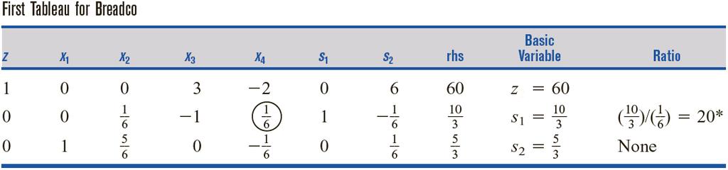
46 The Simplex Method An unbounded LP for a max problem occurs when a variable with a negative coefficient in row 0 has a nonpositive coefficient in each constraint. Example 18 Breadco Bakeries bakes two kinds of bread: French and sourdough. Each loaf of French bread can be sold for 36, and each loaf of sourdough bread for 30. A loaf of French bread requires 1 yeast packet and 6 oz of flour; sourdough requires 1 yeast packet and 5 oz of flour. At present, Breadco has 5 yeast packets and 10 oz of flour. Additional yeast packets can be purchased at 3 each, and additional flour at 4 /oz. Formulate and solve an LP that can be used to maximize Breadco s profits. max 36x x 2 3x 3 4x 4 s.t. x 1 + x 2 x 3 5 6x 1 + 5x 2 x 4 10 x 1, x 2, x 3, x 4 0. Xi Chen (chenxi0109@bfsu.edu.cn) Linear Programming 46 / 148

47 The Simplex Method Xi Chen Linear Programming 47 / 148

48 The Simplex Method For a maximization (minimization) LP problem, the LP will be unbounded iff it has a direction of unboundedness d satisfying cd > 0 (cd < 0). Example 19 The last tableau shows that if we start at the point (5, 0, 0, 20, 0, 0) T, we can find a direction of unboundedness as follows. Every unit by which x 3 is increased will maintain feasibility if we increase x 1 by one unit and x 4 by six units and leave x 2, s 1, and s 2 unchanged. Because we can increase x 3 without limit, this indicates that d = (1, 0, 1, 6, 0, 0) T is a direction of unboundedness. Because cd = (36, 30, 3, 4, 0, 0)(1, 0, 1, 6, 0, 0) T = 9 > 0. we know that LP is unbounded. This follows because each time we move in the direction d an amount that increases x 3 by one unit, we increase z by 9, and we can move as far as we want in the direction d. Lingo Exercise (also refer to Appendix B and C)! Xi Chen (chenxi0109@bfsu.edu.cn) Linear Programming 48 / 148

49 The Simplex Method Definition 2.9 In each of the LP s basic feasible solutions, all of the basic variables are positive. An LP with this property is a nondegenerate LP. An LP is degenerate if it has at least one bfs in which a basic variable is 0. Example 20 Consider the following LP problem max 5x 1 + 2x 2 s.t. x 1 + x 2 6 x 1 x 2 0 x 1, x 2 0 Xi Chen (chenxi0109@bfsu.edu.cn) Linear Programming 49 / 148

50 The Simplex Method It is possible for a sequence of pivots, we encounter the same bfs twice. This occurrence is called cycling. Fortunately, the simplex algorithm can be modified to ensure that cycling will never occur; see Bland (1977). Xi Chen (chenxi0109@bfsu.edu.cn) Linear Programming 50 / 148

51 The Simplex Method It can be shown that for an LP with n decision variables to be degenerate, n + 1 or more of the LP s constraints (including the sign restrictions x i 0 as constraints) must be binding at an extreme point. There may be many sets (maybe hundreds) of basic variables that correspond to some nonoptimal extreme point; see for example point C. The simplex algorithm might encounter all these sets of basic variables before it finds that it was at a nonoptimal extreme point. Xi Chen (chenxi0109@bfsu.edu.cn) Linear Programming 51 / 148

52 The Simplex Method The Big M Method Example 21 Bevco manufactures an orange-flavored soft drink called Oranj by combining orange soda and orange juice. Each ounce of orange soda contains 0.5 oz of sugar and 1 mg of vitamin C. Each ounce of orange juice contains 0.25 oz of sugar and 3 mg of vitamin C. It costs Bevco 2 to produce an ounce of orange soda and 3 to produce an ounce of orange juice. Bevco s marketing department has decided that each 10-oz bottle of Oranj must contain at least 20 mg of vitamin C and at most 4 oz of sugar. Use linear programming to determine how Bevco can meet the marketing department s requirements at minimum cost. Xi Chen (chenxi0109@bfsu.edu.cn) Linear Programming 52 / 148

53 The LP is The Simplex Method min 2x 1 + 3x 2 s.t. 1 2 x x 2 4, x 1 + 3x 2 20, x 1 + x 2 = 10, x 1, x 2 0. We first obtain the following standard form: Row 0 : z 2x 1 3x 2 = 0 Row 1 : 0.5x x 2 + s 1 = 4 Row 2 : x 1 + 3x 2 e 2 = 20 Row 3 : x 1 + x 2 = 10 We simply invent a basic feasible variable for each constraint that needs one (artificial variables), e.g., a i with a i 0. Row 0 : z 2x 1 3x 2 = 0 Row 1 : 0.5x x 2 + s 1 = 4 Row 2 : x 1 + 3x 2 e 2 + a 2 = 20 Row 3 : x 1 + x 2 + a 3 = 10 Xi Chen (chenxi0109@bfsu.edu.cn) Linear Programming 53 / 148

54 The Simplex Method Step 1 Modify the constraints so that the right-hand side of each constraint is nonnegative. Identify each constraint that is now an = or constraint. Step 2 Convert each inequality constraint to standard form. Step 3 If (after step 1 has been completed) constraint i is a = or constraint, add an artificial variable a i with a i 0. Step 4 Let M denote a very large positive number. For each artificial variable, add Ma i ( Ma i ) to the objective function for a min (max) LP problem. Step 5 Because each artificial variable will be in the starting basis, all artificial variables must be eliminated from row 0 before beginning the simplex. This ensures that we begin with a canonical form. Now solve the transformed problem by the simplex. If all artificial variables are equal to zero in the optimal solution, then we have found the optimal solution to the original problem. If any artificial variables are positive in the optimal solution, then the original problem is infeasible. Xi Chen (chenxi0109@bfsu.edu.cn) Linear Programming 54 / 148

55 The Simplex Method Xi Chen Linear Programming 55 / 148

56 The Simplex Method If any artificial variable is positive in the optimal Big M tableau, then the original LP has no feasible solution. min 2x 1 + 3x 2 s.t. 1 2 x x 2 4, x 1 + 3x 2 36, x 1 + x 2 = 10, x 1, x 2 0. Xi Chen (chenxi0109@bfsu.edu.cn) Linear Programming 56 / 148

57 The Simplex Method The Two-Phase Simplex Method Step 1 Modify the constraints so that the right-hand side of each constraint is nonnegative. This requires that each constraint with a negative right-hand side be multiplied through by 1. Step 2 Convert each inequality constraint to the standard form. If constraint i is a constraint, add a slack variable s i. If constraint i is a constraint, subtract an excess variable e i. Step 3 If constraint i is a or = constraint, add an artificial variable a i. Also add the sign restriction a i 0. Step 4 For now, ignore the original LP s objective function. Instead solve an LP whose objective function is min w = sum of all the artificial variables. This is called the Phase I LP. The act of solving the Phase I LP will force the artificial variables to be zero. Xi Chen (chenxi0109@bfsu.edu.cn) Linear Programming 57 / 148

58 The Simplex Method Because each a i 0, solving the Phase I LP will result in one of the following three cases: Case 1 The optimal value of w is greater than zero. In this case, the original LP has no feasible solution. Case 2 The optimal value of w is equal to zero, and no artificial variables are in the optimal Phase I basis. In this case, drop all columns in the optimal Phase I tableau that correspond to the artificial variables. Combine the original objective function with the constraints from the optimal Phase I tableau. This yields the Phase II LP. The optimal solution to the Phase II LP is the optimal solution to the original LP. Case 3 The optimal value of w is equal to zero and at least one artificial variable is in the optimal Phase I basis. In this case, find the optimal solution to the original LP if, at the end of Phase I, we drop all nonbasic artificial variables and any variable from the original problem that has a negative coefficient in row 0 of the optimal Phase I tableau. Xi Chen (chenxi0109@bfsu.edu.cn) Linear Programming 58 / 148

59 The Simplex Method Example 22 (Case 2) min 2x 1 + 3x 2 s.t. 1 2 x x 2 4, x 1 + 3x 2 20, x 1 + x 2 = 10, x 1, x 2 0. Xi Chen (chenxi0109@bfsu.edu.cn) Linear Programming 59 / 148

60 The Simplex Method No artificial variables are in the optimal Phase I basis, so the problem is an example of Case 2. We now drop the columns for the artificial variables a 2 and a 3 and reintroduce the original objective function. It can be observed that the initial Phase II tableau is readily optimal. Thus, in this problem, Phase II requires no pivots to find an optimal solution and we have z = 25, x 1 = 5, x 2 = 5, s 1 = 1 4, e 2 = 0. If the Phase II row 0 does not indicate an optimal tableau, then simply continue with the simplex until an optimal row 0 is obtained. Xi Chen (chenxi0109@bfsu.edu.cn) Linear Programming 60 / 148

61 The Simplex Method Example 23 (Case 1) min 2x 1 + 3x 2 s.t. 1 2 x x 2 4, x 1 + 3x 2 36, x 1 + x 2 = 10, x 1, x 2 0. Xi Chen (chenxi0109@bfsu.edu.cn) Linear Programming 61 / 148

62 The Simplex Method Example 24 (Case 3) min 40x x 2 + 7x x 6 s.t. x 1 x 2 + 2x 5 = 0 2x 1 + x 2 2x 5 = 0 x 1 + x 3 + x 5 x 6 = 3 2x 2 + x 3 + x 4 + 2x 5 + x 6 = 4 x i 0 Use x 4 as a basic variable for the fourth constraint and use artificial variables a 1, a 2, and a 3 as basic variables for the first three constraints. Xi Chen (chenxi0109@bfsu.edu.cn) Linear Programming 62 / 148

63 The Simplex Method We deliberately choose to enter x 3 rather than x 5 into the basis (as a basic variable in row 3), which will immediately yield w = 0. The only original variable with a negative coefficient in the optimal Phase I tableau is x 1, so we may drop x 1 from all future tableaus. As the objective function z = 40x x 2 + 7x x 6 contains no basic variables, our initial tableau for Phase II is Xi Chen (chenxi0109@bfsu.edu.cn) Linear Programming 63 / 148

64 The Simplex Method We now enter x 6 into the basis in row 4 and obtain the optimal tableau shown below z = 7, x 3 = 7 2, x 4 = 1 2, x 2 = x 5 = x 6 = x 3 = 0. Xi Chen (chenxi0109@bfsu.edu.cn) Linear Programming 64 / 148

65 The Simplex Method Unrestricted-in-Sign Variables For each urs variable x i, we begin by defining two new variables x i and x Then substitute x i x i for x i in each constraint and in the objective function. Also add the sign restrictions x i 0 and x i 0. For any bfs, each urs variable x i must fall into one of the following three cases: Case 1 x i > 0 and x i = 0. This case occurs if a bfs has x i > 0. In this case, x i = x i x i = x i. Case 2 x i = 0 and x i > 0. This case occurs if a bfs has x i < 0. In this case, x i = x i x i = x i. Case 3 x i = 0 and x i = 0. This case occurs if a bfs has x i = 0. Example 25 A baker has 30 oz of flour and 5 packages of yeast. Baking a loaf of bread requires 5 oz of flour and 1 package of yeast. Each loaf of bread can be sold for 30. The baker may purchase additional flour at 4 /oz or sell leftover flour at the same price. Formulate and solve an LP to help the baker maximize profits (revenues costs). i. Xi Chen (chenxi0109@bfsu.edu.cn) Linear Programming 65 / 148

66 The Simplex Method Define x 1 = number of loaves of bread baked, x 2 = number of ounces by which flour supply is increased by cash transactions. After noting that x 1 0 and x 2 is urs, the appropriate LP is min 30x 1 4x 2 s.t. 5x x 2, x 1 5, x 1 0, x 2 urs. min 30x 1 4x 2 + 4x 2 s.t. 5x x 2 x 2, x 1 5, x 1, x 2, x 2 0. No matter how many pivots we make, the x 2 column will always be the negative of the x 2 column. Xi Chen (chenxi0109@bfsu.edu.cn) Linear Programming 66 / 148

67 The Simplex Method Example 26 (Modeling Production-Smoothing Costs) Self-learning Xi Chen Linear Programming 67 / 148

68 The Simplex Method Karmarkar s Method for Solving LPs Self-learning! Xi Chen (chenxi0109@bfsu.edu.cn) Linear Programming 68 / 148

69 The Simplex Method Goal Programming in the Absence of Uncertainty Example 27 The Leon Burnit Advertising Agency is trying to determine a TV advertising schedule for Priceler Auto Company. Priceler has three goals: Goal 1 Its ads should be seen by at least 40 million high-income men. Goal 2 Its ads should be seen by at least 60 million low-income people. Goal 3 Its ads should be seen by at least 35 million high-income women. Three types of people in three goals will be referred to as HIM, LIP and HIW, respectively, in the following context. Leon Burnit can purchase two types of ads: those shown during football games and those shown during soap operas. At most, $600, 000 can be spent on ads. The advertising costs and potential audiences of a one-minute ad of each type are shown in the table. Determine how many football ads and soap opera ads to purchase for Priceler. Xi Chen (chenxi0109@bfsu.edu.cn) Linear Programming 69 / 148

70 The Simplex Method Let x 1 = number of minutes of ads shown during football games, and x 2 = number of minutes of ads shown during soap operas. Then any feasible solution to the following LP would meet Priceler s goals: min (or max) 0x 1 + 0x 2 (or any other objective function) s.t. 7x 1 + 3x 2 40, 10x 1 + 5x 2 60, 5x 1 + 4x 2 35, 100x x 2 600, x 1, x 2 0. Xi Chen (chenxi0109@bfsu.edu.cn) Linear Programming 70 / 148

71 The Simplex Method It is impossible to meet all of Priceler s goals, so Burnit might ask Priceler to identify, for each goal, a cost (per-unit short of meeting each goal) that is incurred for failing to meet the goal. Suppose Priceler determines that Each million exposures by which Priceler falls short of the HIM goal costs Priceler a $200, 000 penalty because of lost sales. Each million exposures by which Priceler falls short of the LIP goal costs Priceler a $100, 000 penalty because of lost sales. Each million exposures by which Priceler falls short of the HIW goal costs Priceler a $50, 000 penalty because of lost sales. Since we don t know whether the cost-minimizing solution will undersatisfy or oversatisfy a given goal, define the deviational variables s + i = amount by which we numerically exceed the ith goal, and s i = amount by which we are numerically under the ith goal. 7x 1 + 3x 2 + s 1 s+ 1 10x 1 + 5x 2 + s 2 s+ 2 5x 1 + 4x 2 + s 3 s+ 3 = 40 (HIM constraint) = 60 (LIP constraint) = 35 (HIW constraint) Xi Chen (chenxi0109@bfsu.edu.cn) Linear Programming 71 / 148

72 The Simplex Method Example 28 The objective function coefficient for the variable associated with goal i is called the weight for goal i. min 200s s s 3 s.t. 7x 1 + 3x 2 + s1 s+ 1 = 40 10x 1 + 5x 2 + s 2 s+ 2 = 60 5x 1 + 4x 2 + s 3 s+ 3 = x x all variables are nonnegative. The optimal solution to this LP is z = 250, x 1 = 6, s 1 + = 2, s 3 = 5, and x 2 = s 2 + = s+ 3 = s 1 = s 2 = 0. This meets goal 1 and goal 2 (the goals with the highest costs, or weights, for each unit of deviation from the goal) but fails to meet the least important goal (goal 3). Xi Chen (chenxi0109@bfsu.edu.cn) Linear Programming 72 / 148

73 The Simplex Method Preemptive Goal Programming The decision maker must rank his or her goals from the most important (goal 1) to least important (goal n). The objective function coefficient for the variable representing goal i will be P i. We assume that P 1 P 2 P 3... P n. Define z i = objective function term involving goal i, e.g., z i = P i s i for Example 28. Then preemptive goal programming problems can be solved by an extension of the simplex known as the goal programming simplex. For Example 28, we find that BV = {s 1, s 2, s 3, s 4} is a starting bfs. As with the regular simplex, we must first eliminate all variables in the starting basis from each row 0. Xi Chen (chenxi0109@bfsu.edu.cn) Linear Programming 73 / 148

74 The Simplex Method The goal programming simplex can be described as follows: The goal programming simplex requires n row 0 s (one for each goal). Find the highest-priority goal i having z i > 0. Find the variable with the most positive coefficient in row 0 (goal i ) and enter this variable into the basis. If a variable has a negative coefficient in row 0 associated with a goal having a higher priority than i, then the variable cannot enter the basis since entering such a variable in the basis would increase the deviation from some higher-priority goal. If the variable with the most positive coefficient in row 0 (goal i ) cannot enter the basis, then try another one with a positive coefficient. If no variable for row 0 (goal i ) can enter the basis, then move on to row 0 (goal i + 1) in an attempt to come closer to meeting goal i + 1. When a pivot is performed, row 0 for each goal must be updated. A tableau will yield the optimal solution if all goals are satisfied (that is, z 1 = z 2 =... = z n = 0), or if each variable that can enter the basis and reduce the value of z i for an unsatisfied goal i will increase the deviation from some goal i having a higher priority than goal i. Xi Chen (chenxi0109@bfsu.edu.cn) Linear Programming 74 / 148

75 The Simplex Method Xi Chen Linear Programming 75 / 148

76 The Simplex Method By reordering the priorities assigned to the goals, many solutions can be generated. The decision maker can choose a solution that she feels best fits her preferences; see Lingo Exercise. Xi Chen (chenxi0109@bfsu.edu.cn) Linear Programming 76 / 148

77 Sensitivity Analysis 1 Introduction 2 The Simplex Method 3 Sensitivity Analysis 4 Duality Theory Xi Chen (chenxi0109@bfsu.edu.cn) Linear Programming 77 / 148

78 Sensitivity Analysis A Graphical Introduction to Sensitivity Analysis Definition 3.1 Sensitivity analysis is concerned with how changes in an LP s parameters affect the optimal solution. Reconsider the Giapetto problem: max 3x 1 + 2x 2 s.t. 2x 1 + x 2 100, x 1 + x 2 80, x 1 40, x 1, x 2 0. The optimal solution is z = 180, x 1 = 20, x 2 = 60. How would changes in the problem s objective function coefficients or right-hand sides change this optimal solution? Xi Chen (chenxi0109@bfsu.edu.cn) Linear Programming 78 / 148

79 Sensitivity Analysis Let c 1 be the contribution to profit by each soldier. For what values of c 1 does the current basis remain optimal? If a change in c 1 causes the isoprofit lines to be flatter than the carpentry constraint, then the optimal solution will change from the current optimal solution (point B) to a new optimal solution (point A). Xi Chen (chenxi0109@bfsu.edu.cn) Linear Programming 79 / 148

80 Sensitivity Analysis Let b 1 be the number of available finishing hours. Currently, b 1 = 100. For what values of b 1 does the current basis remain optimal? As long as the point where the finishing and carpentry constraints are binding remains feasible, the optimal solution will still occur where the finishing and carpentry constraints intersect. Xi Chen (chenxi0109@bfsu.edu.cn) Linear Programming 80 / 148

81 Sensitivity Analysis Although for 80 b 1 120, the current basis remains optimal, the values of the decision variables and the objective function value change. 1 Suppose b 1 changes (as long as 20 20), we have b 1 = { 2x1 + x 2 = x 1 + x 2 = 80 { x1 = 20 + x 2 = 60 2 Suppose b 2 changes (as long as 20 20), we have { { 2x1 + x 2 = 100 b 2 = 80 + x 1 + x 2 = 80 + x1 = 20 x 2 = Suppose b 3 changes (as long as 20), we have b 3 = 40 + { 2x1 + x 2 = 100 x 1 + x 2 = 80 { x1 = 20 x 2 = 60 If we change the right-hand side of a constraint with positive s i or e i in the range where the current basis remains optimal, then the optimal solution to the LP is unchanged. Xi Chen (chenxi0109@bfsu.edu.cn) Linear Programming 81 / 148

82 Shadow Prices Sensitivity Analysis The following definition applies only if the change in the right-hand side of the ith constraint leaves the current basis optimal. Definition 3.2 The shadow price for the ith constraint of an LP is the amount by which the optimal z-value is improved increased (decreased) in a max (min) problem if the right-hand side of the ith constraint is increased by 1. Example 29 If finishing hours are available (assuming the current basis remains optimal), then the LP s optimal solution is x 1 = 20 + and x 2 = 60. Then the optimal z-value will equal 3x 1 + 2x 2 = Thus, as long as the current basis remains optimal, a one-unit increase in the number of available finishing hours will increase the optimal z-value by $1. So the shadow price of the first (finishing hours) constraint is $1. Xi Chen (chenxi0109@bfsu.edu.cn) Linear Programming 82 / 148

83 Sensitivity Analysis Suppose that the current basis remains optimal as we increase the right-hand side of the ith constraint of an LP by b i. max min (New optimal z-value) = (Old optimal z-value) + (Constraint i s shadow price) b i, (New optimal z-value) = (Old optimal z-value) (Constraint i s shadow price) b i. A knowledge of sensitivity analysis often enables the analyst to determine from the original solution how changes in an LP s parameters change its optimal solution. Xi Chen (chenxi0109@bfsu.edu.cn) Linear Programming 83 / 148

84 Sensitivity Analysis The Computer and Sensitivity Analysis Example 30 (maximization) Winco sells four types of products. The resources needed to produce one unit of each and the sales prices are given in the table. Currently, 4, 600 units of raw material and 5, 000 labor hours are available. To meet customer demands, exactly 950 total units must be produced. Customers also demand that at least 400 units of product 4 be produced. Formulate an LP that can be used to maximize Winco s sales revenue. Xi Chen (chenxi0109@bfsu.edu.cn) Linear Programming 84 / 148

85 Sensitivity Analysis Let x i = number of units of product i produced by Winco. Example 31 (minimization) max 4x 1 + 6x 2 + 7x 3 + 8x 4 s.t. x 1 + x 2 + x 3 + x 4 = 950 x x 1 + 3x 2 + 4x 3 + 7x x 1 + 4x 2 + 5x 3 + 6x x 1, x 2, x 3, x 4 0 Tucker Inc. must produce 1, 000 Tucker automobiles. The company has four production plants. The cost of producing a Tucker at each plant, along with the raw material and labor needed, is shown in the table. The autoworkers labor union requires that at least 400 cars be produced at plant 3; 3, 300 hours of labor and 4, 000 units of raw material are available for allocation to the four plants. Formulate an LP whose solution will enable Tucker Inc. to minimize the cost of producing 1, 000 cars. Xi Chen (chenxi0109@bfsu.edu.cn) Linear Programming 85 / 148

86 Sensitivity Analysis Let x i = number of cars produced at plant i. Then, expressing the objective function in thousands of dollars, the appropriate LP is min 15x x 2 + 9x 3 + 7x 4 s.t. x 1 + x 2 + x 3 + x 4 = 1000 x x 1 + 3x 2 + 4x 3 + 5x x 1 + 4x 2 + 5x 3 + 6x x 1, x 2, x 3, x 4 0 Xi Chen (chenxi0109@bfsu.edu.cn) Linear Programming 86 / 148

87 Sensitivity Analysis For each objective function coefficient, this range is given in the OBJECTIVE COEFFICIENT RANGES portion. The ALLOWABLE INCREASE (AI) (ALLOWABLE DECREASE (AD)) section indicates the amount by which an objective function coefficient can be increased (decreased) with the current basis remaining optimal. Definition 3.3 We will refer to the range of variables of c i for which the current basis remains optimal as the allowable range for c i. Example 32 (refer to Example 30) a. Suppose the price of product 2 is increased by 50 per unit. What is the new optimal solution to the LP? b. Suppose the sales price of product 1 is increased by 60 per unit. What is the new optimal solution to the LP? c. Suppose the sales price of product 3 is decreased by 60 per unit. What is the new optimal solution to the LP? Xi Chen (chenxi0109@bfsu.edu.cn) Linear Programming 87 / 148

88 Sensitivity Analysis The REDUCED COST portion gives us information about how changing the objective function coefficient for a nonbasic variable will change the LP s optimal solution. Example 33 (refer to Example 30) The basic variables associated with the optimal solution are x 2, x 3, x 4, and s 4 (the slack for the labor constraint), while the nonbasic variable x 1 has a reduced cost of $1. This implies that if we increase x 1 s objective function coefficient (in this case, the sales price per unit of x 1 ) by exactly $1, then there will be alternative optimal solutions, at least one of which will have x 1 as a basic variable. If we increase x 1 s objective function coefficient by more than $1, then (because the current optimal bfs is nondegenerate) any optimal solution to the LP will have x 1 as a basic variable (with x 1 > 0). Thus, the reduced cost for x 1 is the amount by which x 1 misses the optimal basis. Xi Chen (chenxi0109@bfsu.edu.cn) Linear Programming 88 / 148

89 Sensitivity Analysis Example 34 (refer to Example 31) The basic variables associated with the optimal solution are x 1, x 2, x 3, and s 3 (the slack variable for the labor constraint). Again, the optimal bfs is nondegenerate. The nonbasic variable x 4 has a reduced cost of 7 ($7, 000), so we know that if the cost of producing x 4 is decreased by 7, then there will be alternative optimal solutions. In at least one of these optimal solutions, x 4 will be a basic variable. If the cost of producing x 4 is lowered by more than 7, then (because the current optimal solution is nondegenerate) any optimal solution to the LP will have x 4 as a basic variable (with x 4 > 0). We can determine (at least for a two-variable problem) the range of values for a right-hand side within which the current basis remains optimal. This information is given in the RIGHTHAND SIDE RANGES section. Xi Chen (chenxi0109@bfsu.edu.cn) Linear Programming 89 / 148

90 Sensitivity Analysis Example 35 (refer to Example 30) Currently, the right-hand side of this constraint (call it b 1 ) is 950. The current basis remains optimal if b 1 is decreased by up to 100 (the allowable decrease, or AD, for b 1 ) or increased by up to 50 (the allowable increase, or AI, for b 1 ). Thus, the current basis remains optimal if 850 b We call this the allowable range for b 1. The shadow price for each constraint is found in the DUAL PRICES section. If we increase the right-hand side of the ith constraint by an amount b i a decrease in b i implies that b i < 0 and the new right-hand side value for Constraint i remains within the allowable range for the right-hand side given in the RIGHTHAND SIDE RANGES section of the output, then the optimal z-value can be re-determined after a righthand side is changed. Xi Chen (chenxi0109@bfsu.edu.cn) Linear Programming 90 / 148

91 Sensitivity Analysis Example 36 a. In Example 30, suppose that a total of 980 units must be produced. Determine the new optimal z-value. b. In Example 30, suppose that 4, 500 units of raw material are available. What is the new optimal z-value? What if only 4, 400 units of raw material are available? c. In Example 31, suppose that 4, 100 units of raw material are available. Find the new optimal z-value. d. In Example 31, suppose that exactly 950 cars must be produced. What will be the new optimal z-value? A constraint will always have a nonpositive shadow price; a constraint will always have a nonnegative shadow price; and an = constraint may have a positive, negative, or zero shadow price. For any inequality constraint, the product of the values of the constraint s slack or excess variable and its shadow price must equal 0. Xi Chen (chenxi0109@bfsu.edu.cn) Linear Programming 91 / 148

92 Sensitivity Analysis For constraints with nonzero slack or excess, the value of the slack or excess variable is related to the ALLOWABLE INCREASE (DECREASE) sections of the RIGHTHAND SIDE RANGES portion. Example 37 (Degeneracy) max 6x 1 + 4x 2 + 3x 3 + 2x 4 s.t. 2x 1 + 3x 2 + x 3 + 2x x 1 + x 2 + 2x 3 + x x 1 + x 2 + x x x 1 + x 2 + x 4 250, x 1, x 2, x 3, x 4 0 Xi Chen (chenxi0109@bfsu.edu.cn) Linear Programming 92 / 148

93 Sensitivity Analysis According to the output, three oddities that may occur when the optimal solution is degenerate. Oddity 1 In the RANGES IN WHICH THE BASIS IS UNCHANGED, at least one constraint will have a 0 AI or AD. This means that for at least one constraint, the DUAL PRICE can tell us about the new z-value for either an increase or decrease in the righthand side, but not both. Oddity 2 For a nonbasic variable to become positive, its objective function coefficient may have to be improved by more than its REDUCED COST. Oddity 3 Increasing a variable s objective function coefficient by more than its AI or decreasing it by more than its AD may leave the optimal solution to the LP the same. Oddity 2 and oddity 3 occur because the increase changes the set of basic variables but not the LP s optimal solution. Managerial Use of Shadow Prices Self-learning! Xi Chen (chenxi0109@bfsu.edu.cn) Linear Programming 93 / 148

94 Sensitivity Analysis Optimal z-value as a Function of a Constraint s rhs Definition 3.4 For any LP, a graph of the optimal objective function value as a function of a righthand side will consist of several straight-line segments of possibly differing slopes. Such a function is called a piecewise linear function. The slope of each straight-line segment is the constraint s shadow price. Xi Chen (chenxi0109@bfsu.edu.cn) Linear Programming 94 / 148

95 Sensitivity Analysis Example 38 (refer to Example 30) From the following figure, we find that if the amount of available raw material is 3, 900, then the shadow price (or dual price) for raw material is now $2, and the optimal z-value is 5, 400. The current basis remains optimal until rm = 4, 450; between rm = 3, 900 and rm = 4, 450, each unit increase in rm will increase the optimal z-value by the shadow price of $2. Xi Chen (chenxi0109@bfsu.edu.cn) Linear Programming 95 / 148

96 Sensitivity Analysis Example 39 (contd.) When rm = 4, 450, x 3 enters the basis and x 1 exits. The shadow price of rm is now $1, and each additional unit of rm (up to the next change of basis) will increase the optimal z-value by $1. The next basis change occurs when rm = 4, 850. At this point, the new optimal z-value may be computed as (optimal z-value for rm = $6, 500) + (4, 850 4, 450)($1) = $6, 900. When rm = 4, 850, we pivot in SLACK3 (the slack variable for row 3 or constraint 2), and SLACK5 exits. The new shadow price for rm is $0. Thus when rm = 4, 850, we see that an additional unit of rm will not increase the optimal z-value. Xi Chen (chenxi0109@bfsu.edu.cn) Linear Programming 96 / 148

97 Sensitivity Analysis For a constraint in a maximization problem, the slope of each line segment must be nonnegative more of a resource can t hurt; the slopes of successive line segments for a constraint will be nonincreasing, which is simply a consequence of diminishing returns. For a constraint in a maximization problem, the slope of each line segment will be nonpositive; the slopes of successive line segments will be nonincreasing. Xi Chen (chenxi0109@bfsu.edu.cn) Linear Programming 97 / 148

98 Sensitivity Analysis For an = constraint in a maximization problem, the graph of the optimal z-value as a function of right-hand side will again be piecewise linear. The slopes of each line segment may be positive or negative, but the slopes of successive line segments will again be nonincreasing. For the constraint x 1 + x 2 + x 3 + x 4 = 950 in Example 30, we obtain the graph in the following figure. Xi Chen (chenxi0109@bfsu.edu.cn) Linear Programming 98 / 148

99 Sensitivity Analysis Optimal z-value as a Function of an Objective Function Coefficient Example 40 Reconsider the Giapetto problem. max 3x 1 + 2x 2 s.t. 2x 1 + x 2 100, x 1 + x 2 80, x 1 40, x 1, x 2 0 Let c 1 = objective function coefficient for x 1. A typical isoprofit line is c 1 x 1 + 2x 2 = k, so we know that the slope of a typical isoprofit line is c 1 /2. Thus, point B = (20, 60) is optimal if 2 c 1 /2 1. Value of c 1 Optimal z-value 0 c 1 2 c 1 (0) + 2(80) = $160 2 c 1 4 c 1 (20) + 2(60) = $ c 1 c 1 4 c 1 (40) + 2(20) = $ c 1 Xi Chen (chenxi0109@bfsu.edu.cn) Linear Programming 99 / 148

100 Sensitivity Analysis In a maximization problem, the graph of the optimal z-value as a function of c 1 is a piecewise linear function, and the optimal z-value will be a nondecreasing, piecewise linear function of an objective function coefficient; the slope of each line segment in the graph is equal to the value of x 1 in the optimal solution, and the slope will be a nondecreasing function of the objective function coefficient. Xi Chen (chenxi0109@bfsu.edu.cn) Linear Programming 100 / 148

101 Sensitivity Analysis Assume that we are solving a max problem that has been prepared for solution by the Big M method and that at this point, the LP has m constraints and n variables. max c 1 x 1 + c 2 x c n x n s.t. a 11 x 1 + a 12 x a 1n x n = b 1 a 21 x 1 + a 22 x a 2n x n = b 2 a m1 x 1 + a m2 x a mn x n = b m x i 0, i = 1, 2,..., n Use the Dakota Furniture problem as an example.... (2) max 60x x x 3 + 0s 1 + 0s 2 + 0s 3 s.t. 8x 1 + 6x 2 + x 3 + s 1 = 48 4x 1 + 2x x 3 + s 2 = 20 2x x x 3 + s 3 = 8 x 1, x 2, x 3, s 1, s 2, s 3 0 Xi Chen (chenxi0109@bfsu.edu.cn) Linear Programming 101 / 148

102 Sensitivity Analysis Definition 3.5 Define BV = {BV 1, BV 2,..., BV m } to be the set of basic variables in the optimal tableau, and let the m 1 vector x BV = (x BV1, x BV2,..., x BVm ) T. The set NBV and the (n m) 1 vector x NBV are similarly defined. The optimal tableau for the Dakota problem is z + 5x s s 3 = 280 2x 2 + s 1 + 2s 2 8s 3 = 24 2x 2 + x 3 + 2s 2 4s 3 = 8 x x 2 0.5s s 3 = 2 (3) For this optimal tableau, we have s 1 x BV = x 3 x 1, x NBV = x 2 s 2 s 3. Xi Chen (chenxi0109@bfsu.edu.cn) Linear Programming 102 / 148

103 Sensitivity Analysis Definition 3.6 c BV is the 1 m row vector (c BV1, c BV2,..., c BVm ). c NBV is the 1 (n m) row vector whose elements are the coefficients of the nonbasic variables (in the NBV order). The m m matrix B is the matrix whose jth column is the column for BV j in (2). a j is the column (in the constraints) for the variable x j in (2). N is the m (n m) matrix whose columns are the columns for the nonbasic variables (in the NBV order) in (2). The m 1 vector b is the right-hand side of the constraints in (2). By these definitions, (2) may be written as max s.t. c BV x BV + c NBV x NBV Bx BV + Nx NBV = b x BV, x NBV 0 (4) Xi Chen (chenxi0109@bfsu.edu.cn) Linear Programming 103 / 148

104 Sensitivity Analysis Multiplying the constraints in (4) through by B 1, we obtain x BV + B 1 Nx NBV = B 1 b. (5) For the Dakota problem, we have B 1 = 0 2 4, s x 2 x s 2 x s 3 = From (5), we see that the column of a nonbasic variable x j in the constraints of the optimal tableau is given by B 1 a j, and the right-hand side of the constraints is the vector B 1 b. Xi Chen (chenxi0109@bfsu.edu.cn) Linear Programming 104 / 148

105 Sensitivity Analysis Multiply the constraints (expressed in the form Bx BV + Nx NBV = b) through by the vector c BV B 1, and we have } c BV x BV + c BV B 1 Nx NBV = c BV B 1 b z c BV x BV c NBV x NBV = 0 z + ( c BV B 1 N c NBV ) xnbv = c BV B 1 b. The coefficient of x j in row 0 is c j = c BV B 1 a j c j and the right-hand side of row 0 is c BV B 1 b. Exercise 3.1 Find the coefficient of x j in row 0 in Dakota problem s optimal tableau. Coefficient of s i in optimal row 0 is ith element of c BV B 1. Coefficient of e i in optimal row 0 is -(ith element of c BV B 1 ). Coefficient of a i in optimal row 0 is (ith element of c BV B 1 )+M. Xi Chen (chenxi0109@bfsu.edu.cn) Linear Programming 105 / 148

106 Sensitivity Analysis Exercise 3.2 For the following LP, the optimal basis is BV = {x 2, s 2 }. Compute the optimal tableau. Solution Definition 3.7 max x 1 + 4x 2 s.t. x 1 + 2x 2 6, 2x 1 + x 2 8, x 1, x 2 0. z + x 1 + 2s 1 = x 1 + x s 1 = 3 1.5x 1 0.5s 1 + s 2 = 5 For a maximization LP problem, if it is possible to obtain a better (larger z-value) bfs by pivoting in a nonbasic variable with a negative coefficient in row 0, the BV is a suboptimal basis. If a constraint (or constraints) has a negative right-hand side, the BV is an infeasible basis. Xi Chen (chenxi0109@bfsu.edu.cn) Linear Programming 106 / 148

107 Sensitivity Analysis Changing the Objective Function Coefficient of a Nonbasic Variable Suppose we change the objective function coefficient of x 2 from 30 to For what values of will the current basis remain optimal? Since B 1 and b are unchanged, B 1 b has not changed. Hence, BV is still feasible. Because x 2 is a nonbasic variable, c BV has not changed. The only change is in c 2. Thus, BV will remain optimal if c a 2 = c 2 = c BV B 1 a 2 (30 + ) = 5. Thus, BV will remain optimal, if 5, and the values of the decision variables and the optimal z-value remain unchanged. Xi Chen (chenxi0109@bfsu.edu.cn) Linear Programming 107 / 148

108 Sensitivity Analysis If > 5, BV will no longer be optimal. The new optimal solution can be found by recreating the BV tableau and then using the simplex algorithm. The reduced cost for a nonbasic variable (in a max problem) is the maximum amount by which the variable s objective function coefficient can be increased before the current basis becomes suboptimal, and it becomes optimal for the nonbasic variable to enter the basis. Xi Chen (chenxi0109@bfsu.edu.cn) Linear Programming 108 / 148

109 Sensitivity Analysis Changing the Objective Function Coefficient of a Basic Variable Suppose that c 1 is changed to 60 +, changing c BV to (0, 20, 60 + ). Since B 1 and b are unchanged, B 1 b has not changed. Hence, BV is still feasible. A change in c BV B 1 may change more than one coefficient in row 0. To determine whether BV remains optimal, we must recompute row 0 for the BV tableau B 1 = 0 2 4, c BV B 1 = (0, , ), c 2 = c BV B 1 a 2 c 2 = , c s2 = , c s3 = Therefore, BV will remain optimal iff c 2 0, c s2 0 and c s3 0. We then have The values of the decision variables do not change, but the optimal z-value changes. Xi Chen (chenxi0109@bfsu.edu.cn) Linear Programming 109 / 148

110 Sensitivity Analysis Suppose c 1 = 100 > 80. The current basis is no longer optimal. Simply create the optimal tableau for c 1 = 100 and proceed with the simplex. If the objective function coefficient of a basic variable x j is changed, the current basis remains optimal if the coefficient of every variable in row 0 of the BV tableau remains nonnegative. Otherwise, it is no longer optimal. Xi Chen (chenxi0109@bfsu.edu.cn) Linear Programming 110 / 148

111 Sensitivity Analysis Changing the Right-Hand Side of a Constraint If we change b 2 to 20 +, how the optimal solution to an LP changes if the right-hand side of a constraint is changed? Row 0 of the optimal tableau will not change, and thus the current basis remains optimal. As long as the right-hand side of each constraint in the optimal tableau remains nonnegative, the current basis remains feasible and optimal. If at least one right-hand side in the optimal tableau becomes negative, then the current basis is no longer feasible and therefore no longer optimal. B 1 b = = The current basis will remain optimal iff 4 4. Both the values of the decision variables (B 1 b) and z (c BV B 1 b) change.. Xi Chen (chenxi0109@bfsu.edu.cn) Linear Programming 111 / 148

112 Sensitivity Analysis Suppose we change b 2 to 30 > 24. The current basis is no longer optimal. If we re-create the optimal tableau, unfortunately, such a tableau does not yield a readily apparent basic feasible solution, as shown below. If the right-hand side of a constraint is changed, then the current basis remains optimal if the right-hand side of each constraint in the tableau remains nonnegative; if the right-hand side of any constraint is negative, then the current basis is infeasible, and a new optimal solution must be found. Xi Chen (chenxi0109@bfsu.edu.cn) Linear Programming 112 / 148

113 Sensitivity Analysis Changing the Column of a Nonbasic Variable Suppose that the price of tables increased to $43 and, because of changes in production technology, a table required 5 board feet of lumber, 2 finishing hours, and 2 carpentry hours. Would this change the optimal solution to the Dakota problem? Changing the column for a nonbasic variable such as tables leaves B (and B 1 ) and b unchanged. Hence, BV is still feasible. The only part of row 0 that is changed is c 2, and the current basis will remain optimal iff c 2 0 holds. 5 c 2 = c BV B 1 a 2 c 2 = (0, 10, 10) 2 43 = 3. (price out x 2 ) 2 The fact that c 2 = 3 means that each table that Dakota manufactures now increases revenues by $3. Xi Chen (chenxi0109@bfsu.edu.cn) Linear Programming 113 / 148

114 Sensitivity Analysis To find the new optimal solution, we recreate the tableau for BV = {s 1, x 3, x 1 } and then apply the simplex algorithm. If the column of a basic variable is changed, then it is usually difficult to determine whether the current basis remains optimal since B (and B 1 ) and c BV, and thus the entire row 0 and the entire right-hand side of the optimal tableau change. Xi Chen (chenxi0109@bfsu.edu.cn) Linear Programming 114 / 148

115 Sensitivity Analysis Adding a New Activity Suppose that Dakota is considering making footstools. A stool sells for $15 and requires 1 board foot of lumber, 1 finishing hour, and 1 carpentry hour. Should the company manufacture any stools? z 60x 1 30x 2 20x 3 15x 4 = 0 8x 1 + 6x 2 + x 3 + x 4 + s 1 = 48 4x 1 + 2x x 3 + x 4 + s 2 = 20 2x x x 3 + x 4 + s 3 = 8 The addition of the x 4 column to the problem is adding a new activity. The right-hand sides of all constraints in the optimal tableau will remain unchanged. Hence, BV is still feasible. The only variable in row 0 that can have a negative coefficient is x 4. So the current basis will remain optimal if c 4 0. Since c 4 = c BV B 1 a 4 c 4 = 5 0, the current basis is still optimal. Equivalently, the reduced cost of footstools is $5. Xi Chen (chenxi0109@bfsu.edu.cn) Linear Programming 115 / 148

116 Sensitivity Analysis Therefore, if a new column (corresponding to a variable x j ) is added to an LP, then the current basis remains optimal if c j 0. Xi Chen (chenxi0109@bfsu.edu.cn) Linear Programming 116 / 148

117 Duality Theory 1 Introduction 2 The Simplex Method 3 Sensitivity Analysis 4 Duality Theory Xi Chen (chenxi0109@bfsu.edu.cn) Linear Programming 117 / 148

118 Duality Theory Definition 4.1 Associated with any LP is another LP, called the dual. When taking the dual of a given LP, we refer to the given LP as the primal. A normal max problem may be written as max c 1 x 1 + c 2 x c n x n s.t. a 11 x 1 + a 12 x a 1n x n b 1 a 21 x 1 + a 22 x a 2n x n b 2, x j 0 a m1 x 1 + a m2 x a mn x n b m (6) The dual of a normal max problem (normal min problem) is defined to be min s.t. b 1 y 1 + b 2 y b m y m a 11 y 1 + a 21 y a m1 y m c 1 a 12 y 1 + a 22 y a m2 y m c 2, y i 0 a 1n y 1 + a 2n y a mn y m c n (7) Xi Chen (chenxi0109@bfsu.edu.cn) Linear Programming 118 / 148

119 Duality Theory Finding the Dual of a Normal LP Problem If the primal is a normal max problem, then it can be read across; the dual is found by reading down. If the primal is a normal min problem, we find it by reading down; the dual is found by reading across. Xi Chen (chenxi0109@bfsu.edu.cn) Linear Programming 119 / 148

120 Duality Theory Exercise 4.1 The Dakota problem is max 60x x x 3 s.t. 8x 1 + 6x 2 + x x 1 + 2x x x x x 3 8 We find the Dakota dual to be min 48y y 2 + 8y 3 s.t. 8y 1 + 4y 2 + 2y y 1 + 2y y 3 30 y y y 3 20, x 1, x 2, x 3 0, y 1, y 2, y 3 0 Exercise 4.2 Find the dual of the diet problem. Xi Chen (chenxi0109@bfsu.edu.cn) Linear Programming 120 / 148

121 Duality Theory Finding the Dual of a Nonnormal LP (max) Example 4.1 Find the dual of the following LP: max 2x 1 + x 2 s.t. x 1 + x 2 = 2 2x 1 x 2 3 x 1 x 2 1, x 1 0, x 2 urs (8) Step 1 Multiply each constraint by 1, converting it into a constraint. Step 2 Replace each equality constraint by two inequality constraints (a constraint and a constraint). Then convert the constraint to a constraint. Step 3 Replace each urs variable x i by x i = x i x i, where x i, x i 0. Xi Chen (chenxi0109@bfsu.edu.cn) Linear Programming 121 / 148

122 Duality Theory After these transformations are complete, (8) has been transformed into the following (equivalent) LP: max 2x 1 + x 2 x 2 s.t. x 1 + x 2 x 2 2 x 1 x 2 + x 2 2 2x 1 + x 2 x 2 3 x 1 x 2 + x 2 1, x 1, x 2, x 2 0 (9) Because (9) is a normal max problem, we could use (6) and (7) to find the dual of (9). Exercise 4.3 Find the dual of (8) according to the transformation (9). Xi Chen (chenxi0109@bfsu.edu.cn) Linear Programming 122 / 148

123 Duality Theory We can also find the dual of a nonnormal LP without going through the transformations by using the following rules: Step 1 Fill in table so that the primal can be read across. Step 2 After making the following changes, the dual can be read down in the usual fashion: (a). If the ith primal constraint is a constraint, then the corresponding dual variable y i must satisfy y i 0. (b). If the ith primal constraint is an equality constraint, then the dual variable y i is now unrestricted in sign. (c). If the ith primal variable is urs, then the ith dual constraint will be an equality constraint. Xi Chen (chenxi0109@bfsu.edu.cn) Linear Programming 123 / 148

124 Duality Theory Economic Interpretation of the Dual Problem The dual of the Dakota problem is min 48y y 2 + 8y 3 s.t. 8y 1 + 4y 2 + 2y 3 60 (Desk constraint) 6y 1 + 2y y 3 30 (Table constraint) y y y 3 20 (Chair constraint) y 1, y 2, y 3 0 Suppose an entrepreneur wants to purchase all of Dakota s resources. Then the entrepreneur must determine the price he or she is willing to pay for a unit of each of Dakota s resources. In setting resource prices, resource prices must be set high enough to induce Dakota to sell. When the primal is a normal max problem, the dual variables are related to the value of the resources available to the decision maker. For this reason, the dual variables are often referred to as resource shadow prices. Xi Chen (chenxi0109@bfsu.edu.cn) Linear Programming 124 / 148

125 Duality Theory Suppose Candice is a nutrient salesperson who sells calories, chocolate, sugar, and fat. She wants to ensure that a dieter will meet all of his or her daily requirements by purchasing calories, sugar, fat, and chocolate. In setting nutrient prices, Candice must set prices low enough so that it will be in the dieter s economic interest to purchase all nutrients from her. In summary, when the primal is a normal max problem or a normal min problem, the dual problem has an intuitive economic interpretation. Xi Chen (chenxi0109@bfsu.edu.cn) Linear Programming 125 / 148

126 Duality Theory The Dual Theorem and Its Consequences The primal may be written as follows: max s.t. c 1 x 1 + c 2 x c n x n a 11 x 1 + a 12 x a 1n x n b 1 a 21 x 1 + a 22 x a 2n x n b a m1 x 1 + a m2 x a mn x n b m x j 0, (j = 1, 2,..., n) The dual may be written as follows: min b 1 y 1 + b 2 y b m y m s.t. a 11 y 1 + a 21 y a m1 y m c 1 a 12 y 1 + a 22 y a m2 y m c a 1n y 1 + a 2n y a mn y m c n y i 0, (i = 1, 2,..., m) Xi Chen (chenxi0109@bfsu.edu.cn) Linear Programming 126 / 148

127 Duality Theory Lemma 4.1 (Weak Duality) Let x = (x 1, x 2,..., x n ) T be any feasible solution to the primal and y = (y 1, y 2,..., y m ) T be any feasible solution to the dual. Then (z-value for x) (w-value for y). Proof. Because y i 0, multiplying the ith primal constraint in the primal by y i will yield the following valid inequality: y i a i1 x 1 + y i a i2 x y i a in x n b i y i, (i = 1, 2,..., m). Adding the m inequalities, we have m n y i a ij x j i=1 j=1 m b i y i. i=1 Xi Chen (chenxi0109@bfsu.edu.cn) Linear Programming 127 / 148

128 Duality Theory contd. Similarly, we can derive n m x j a ji y i j=1 i=1 n c j x j. j=1 Therefore, we obtain the result n c j x j j=1 n m x j a ji y i = j=1 i=1 m n y i a ij x j i=1 j=1 m b i y i. i=1 If a feasible solution to either the primal or the dual is readily available, weak duality can be used to obtain a bound on the optimal objective function value for the other problem. Xi Chen (chenxi0109@bfsu.edu.cn) Linear Programming 128 / 148

129 Duality Theory Lemma 4.2 Let x = (x 1, x 2,..., x n ) T be a feasible solution to the primal and y = (y 1, y 2,..., y m ) be a feasible solution to the dual. If cx = yb, then x is optimal for the primal and y is optimal for the dual. Proof. From weak duality we know that for any primal feasible point x, cx yb. Thus, any primal feasible point must yield a z-value that does not exceed yb. Because x is primal feasible and has a primal objective function value of cx = yb, x must be primal optimal. Similarly, y must be an optimal solution for the dual. Exercise 4.4 Show that if the primal is unbounded, then the dual problem is infeasible; and if the dual is unbounded, then the primal is infeasible. Xi Chen (chenxi0109@bfsu.edu.cn) Linear Programming 129 / 148

130 Duality Theory Theorem 4.1 Suppose BV is an optimal basis for the primal. Then c BV B 1 is an optimal solution to the dual. Also, z = w. Proof. After adding slack variables s 1, s 2,..., s m to the primal, we write the primal and dual problems as follows: max s.t. c 1 x 1 + c 2 x c n x n a 11 x 1 + a 12 x a 1n x n +s 1 = b 1 a 21 x 1 + a 22 x a 2n x n +s 2 = b a m1 x 1 + a m2 x a mn x n +s m = b m x j 0, (j = 1, 2,..., n), s i 0, (i = 1, 2,..., m) Xi Chen (chenxi0109@bfsu.edu.cn) Linear Programming 130 / 148

131 Duality Theory contd. min s.t. b 1 y 1 + b 2 y b m y m a 11 y 1 + a 21 y a m1 y m c 1 a 12 y 1 + a 22 y a m2 y m c a 1n y 1 + a 2n y a mn y m c n y i 0, (i = 1, 2,..., m) Let BV be an optimal basis for the primal, and c BV B 1 = (y 1, y 2,..., y m ). Thus, for the optimal basis BV, y i is the ith element of c BV B 1. Xi Chen (chenxi0109@bfsu.edu.cn) Linear Programming 131 / 148

132 Duality Theory contd. Since BV is optimal the primal, the coefficient of each variable in row 0 of BV s primal tableau must be nonnegative, i.e., for j = 1, 2,..., n, c j = c BV B 1 a j c j = (y 1, y 2,..., y m ) a 1j a 2j. a mj c j = Thus, c BV B 1 satisfies each of the n dual constraints. m y i a ij c j 0. Because BV is an optimal basis for the primal, we also know that each slack variable has a nonnegative coefficient in the BV primal tableau. The coefficient of s i in BV s row 0 is y i, the ith element of c BV B 1. Hence, y i 0 for i = 1, 2,..., m. Consequently, c BV B 1 is indeed dual feasible. i=1 Xi Chen (chenxi0109@bfsu.edu.cn) Linear Programming 132 / 148

133 Duality Theory contd. The primal objective function value for BV is c BV B 1 b. But the dual objective function value for the dual feasible solution c BV B 1 is b 1 m m b 2 b i y i = y i b i = (y 1, y 2,..., y m ) i=1 i=1. = c BV B 1 b. b m Hence, dual objective function value for c BV B 1 is equal to primal objective function value for BV. By Lemma 4.2, we can conclude that c BV B 1 is optimal for the dual and z = w. Exercise 4.5 If the primal is a normal max problem, then the optimal value of the ith dual variable is the coefficient of s i in row 0 of the optimal primal tableau. What if the primal has (e i ) or equality constraints? Xi Chen (chenxi0109@bfsu.edu.cn) Linear Programming 133 / 148

134 Duality Theory Definition 4.2 The shadow price of the ith constraint is the amount by which the optimal z-value is improved (increased in a max problem and decreased in a min problem) if we increase b i by 1 (from b i to b i + 1). The shadow price of the ith constraint of a max problem is the optimal value of the ith dual variable. Exercise 4.6 For the Dakota problem: 1 Find and interpret the shadow prices. 2 If 18 finishing hours were available, what would be Dakota s revenue? 3 If 9 carpentry hours were available, what would be Dakota s revenue? 4 If 30 board feet of lumber were available, what would be Dakota s revenue? 5 If 30 carpentry hours were available, why couldn t the shadow price for the carpentry constraint be used to determine the new z-value? Xi Chen (chenxi0109@bfsu.edu.cn) Linear Programming 134 / 148

135 Duality Theory Intuitive Explanation of the Sign of Shadow Prices Since the shadow prices are the dual variables, the shadow price for a constraint will be nonnegative; for a constraint, nonpositive; and for an equality constraint, unrestricted in sign. Adding points to the feasible region of a max problem cannot decrease the optimal z-value. Example 41 For the Dakota problem, if we increase the right-hand side of the carpentry constraint by 1 (from 8 to 9), we see that all points that were originally feasible remain feasible, and some new points (which use > 8 and 9 carpentry hours) may be feasible. Thus, the optimal z-value cannot decrease, and the shadow price for the carpentry constraint must be nonnegative. Shadow price can be viewed as a premium over the cost of the resource a company would be willing to pay for an extra unit! Xi Chen (chenxi0109@bfsu.edu.cn) Linear Programming 135 / 148

136 Duality Theory Shadow Prices for and = Constraints Example 42 Steelco has received an order for 100 tons of steel. The order must contain at least 3.5 tons of nickel, at most 3 tons of carbon, and exactly 4 tons of manganese. Steelco receives $20/ton for the order. To fill the order, Steelco can combine four alloys, whose chemical composition is given in the following table. Steelco wants to maximize the profit (revenues - costs) obtained from filling the order. Formulate the appropriate LP. Also find and interpret the shadow prices for each constraint. Xi Chen (chenxi0109@bfsu.edu.cn) Linear Programming 136 / 148

137 Duality Theory Duality and Sensitivity Analysis Corollary 4.1 By the proof of Theorem 4.1, assuming that a set of basic variables BV is feasible, then BV is optimal (that is, each variable in row 0 has a nonnegative coefficient) if and only if the associated dual solution (c BV B 1 ) is dual feasible. This result be used for an alternative way of doing the following types of sensitivity analysis: Change 1 Changing the objective function coefficient of a nonbasic variable Change 2 Changing the column of a nonbasic variable Change 3 Adding a new activity The above changes will leave the current basis optimal if and only if the current dual solution c BV B 1 remains dual feasible. Xi Chen (chenxi0109@bfsu.edu.cn) Linear Programming 137 / 148

138 The Dakota problem is Duality Theory max 60x x x 3 s.t. 8x 1 + 6x 2 + x 3 48 (Lumber constraint) 4x 1 + 2x x 3 20 (Finishing constraint) 2x x x 3 8 (Carpentry constraint) x 1, x 2, x 3 0 The optimal primal solution was z = 280, s 1 = 24, x 3 = 8, x 1 = 2, x 2 = 0, s 2 = 0, s 3 = 0. min 48y y 2 + 8y 3 s.t. 8y 1 + 4y 2 + 2y 3 60 (Desk constraint) 6y 1 + 2y y 3 30 (Table constraint) y y y 3 20 (Chair constraint) y 1, y 2, y 3 0 The optimal dual solution and therefore the constraint shadow prices are y 1 = 0, y 2 = 10, y 3 = 10. Xi Chen (chenxi0109@bfsu.edu.cn) Linear Programming 138 / 148

139 Duality Theory Changing the objective function coefficient of a nonbasic variable Example 43 Let c 2 be the coefficient of x 2 (tables) in the Dakota objective function. In other words, c 2 is the price at which a table is sold. For what values of c 2 will the current basis remain optimal? Changing the column for a nonbasic activity Example 44 Suppose a table sells for $43 and uses 5 board feet of lumber, 2 finishing hours, and 2 carpentry hours. Does the current basis remain optimal? Adding a new activity Example 45 Suppose Dakota is considering manufacturing footstools (x 4 ). A footstool sells for $15 and uses 1 board foot of lumber, 1 finishing hour, and 1 carpentry hour. Does the current basis remain optimal? Xi Chen (chenxi0109@bfsu.edu.cn) Linear Programming 139 / 148

140 Duality Theory Complementary Slackness Theorem 4.2 Assume that the primal is a normal max problem with m constraints and corresponding slack variables s i, (i = 1, 2,..., m). Then the dual is a normal min problem with n constraints and corresponding excess variables e j, (j = 1, 2,..., n). Let x = (x 1, x 2,..., x n ) T and y = (y 1, y 2,..., y m ) T be a feasible primal solution and feasible dual solution, respectively. Then x is primal optimal and y is dual optimal if and only if s i y i = 0, (i = 1, 2,..., m) and e j x j = 0, (j = 1, 2,..., n). A constraint in either the primal or dual is nonbinding (has either s i > 0 or e j > 0), then the corresponding variable in the other (or complementary) problem must equal 0. Hence the name complementary slackness. Exercise 4.7 Verify Theorem 4.2 for the Dakota problem. Xi Chen (chenxi0109@bfsu.edu.cn) Linear Programming 140 / 148

141 Duality Theory For any variable x j in the optimal primal basis, the marginal revenue obtained from producing a unit of x j must equal the marginal cost of the resources used to produce a unit of x j. x 1 > 0 means that desks are in the optimal basis. Marginal revenue obtained by manufacturing desk is $60. Cost of lumber in desk is zero. Cost of finishing hours used to make a desk is $40. Cost of carpentry hours used to make a desk is $20. If the optimal solution to the primal or dual is known, complementary slackness can sometimes be used to determine the optimal solution to the complementary problem. Example 46 Suppose we were told that the optimal solution to the Dakota problem was z = 280, x 1 = 2, x 2 = 0, x 3 = 8, s 1 = 24, s 2 = 0, s 3 = 0. Can we use Theorem 4.2 to help us find the optimal solution to the Dakota dual? Xi Chen (chenxi0109@bfsu.edu.cn) Linear Programming 141 / 148

142 Duality Theory The Dual Simplex Method (max) Suppose the initial simplex tableau is dual feasible. Step 1 Is the right-hand side of each constraint nonnegative? If so, an optimal solution has been found; if not, at least one constraint has a negative right-hand side, and we go to step 2. Step 2 Choose the most negative basic variable as the variable to leave the basis. The row in which the variable is basic will be the pivot row. To select the variable that enters the basis, we compute the following ratio for each variable x j that has a negative coefficient in the pivot row, and choose the one with the smallest ratio (absolute value): Coefficient of x j in row 0 Coefficient of x j in pivot row. Step 3 If there is any constraint in which the right-hand side is negative and each variable has a nonnegative coefficient, then the LP has no feasible solution. If no constraint indicating infeasibility is found, return to step 1. Xi Chen (chenxi0109@bfsu.edu.cn) Linear Programming 142 / 148

143 Duality Theory Finding the New Optimal Solution after a Constraint is Added to an LP When a constraint is added, one of the following three cases will occur: The current optimal solution satisfies the new constraint, and the current solution remains optimal. The current solution is no longer feasible, so it can no longer be optimal. The dual simplex method can be used to determine the new optimal solution. The current solution is z = 280, x 1 = 2, x 2 = 0, x 3 = 8. Xi Chen (chenxi0109@bfsu.edu.cn) Linear Programming 143 / 148

144 Duality Theory The additional constraint causes the LP to have no feasible solutions. Step 3 of the dual simplex method allows us to show that the LP is now infeasible. Xi Chen (chenxi0109@bfsu.edu.cn) Linear Programming 144 / 148

145 Duality Theory Hence, the Dakota problem with the additional constraint x 1 + x 2 12 has no feasible solution. Xi Chen (chenxi0109@bfsu.edu.cn) Linear Programming 145 / 148

146 Duality Theory Changing a Right-Hand Side If the rhs of a constraint is changed and the current basis becomes infeasible, the dual simplex can be used to find the new optimal solution. Suppose that 30 finishing hours are now available. Xi Chen (chenxi0109@bfsu.edu.cn) Linear Programming 146 / 148

147 Duality Theory Solving a Normal min Problem Consider the following minimization LP problem: min x 1 + 2x 2 s.t. x 1 2x 2 + x 3 4 2x 1 + x 2 x 3 6 x 1, x 2, x 3 0 We begin by multiplying z by 1 to convert the LP to a max problem with objective function z = x 1 2x 2. After subtracting excess variables e 1 and e 2 from the two constraints, we obtain the initial tableau. Xi Chen (chenxi0109@bfsu.edu.cn) Linear Programming 147 / 148

148 Duality Theory Observe that each dual simplex tableau (except the optimal dual simplex tableau) has a z -value exceeding the optimal z -value. For this reason, we say that the dual simplex tableaus are superoptimal. Xi Chen (chenxi0109@bfsu.edu.cn) Linear Programming 148 / 148