5. Multiple Regression (Regressioanalyysi) (Azcel Ch. 11, Milton/Arnold Ch. 12) The k-variable Multiple Regression Model

Transcription

1 5. Multiple Regression (Regressioanalyysi) (Azcel Ch. 11, Milton/Arnold Ch. 12) The k-variable Multiple Regression Model The population regression model of a dependent variable Y on a set of k independent variables X 1, X 2,..., X k is given by Y = β 0 + β 1 X 1 + β 2 X β k X k + ɛ, where β 0 is the intercept and β i, i = 1,..., k are the slopes of the regression surface (also called response surface) with respect to X i. Model assumptions: 1. ɛ j NID(0, σ 2 ) for all observations j = 1,..., n; 2. The variables X i are considered fixed quantities (not random variables), that is, the only randomness in Y comes from the error term ɛ. The parameters β 0, β 1,... β k are estimated by the method of least squares (pns-menetelmä), as in the case with only 1 regressor. 160

2 Method of Least Squares with k Regressors (Pienimmän neliösumman menetelmä) The following table contains the quantity of a product sold (Y) as a function of the products price (X). Such data may be conveniently illustrated in a so called scatterplot (hajontakuvio). 161

3 It appears, that the number of units sold Y is roughly a linear function of the price X, that is, y j b 0 + b 1 x j, y j = b 0 + b 1 x j + u j, j = , (1) where the residuals (jäännökset) u j are small in some sense compared to the linear term b 0 + b 1 x j. We shall in the following consider a technique of identifying a linear relationship in approximately linearly distributed data, known as Method of Least Squares or Regression Analysis, (pienimmän neliösumman menetelmä, regressioanalyysi). or 162

4 Before doing that, let us rewrite the regression equation (1) in matrix form as y (25 1) = X (25 2) b (2 1) + u (25 1), where: (2) y = X= b= ( b0 b 1 ) u 1 u 2 u 3 u=. u 24 u 25 Doing so has the advantage that we may easily generalize our method to the case where the dependent variable Y, called regressand (selitettävä muuttuja), depends linearly on more than one independent variable X, called regressor (selittävä muuttuja). For example, the number of units sold might not only depend on a constant (X 1 = 1) and price (X 2 ), but also on advertisement (X 3 ), bonuses to sales officers (X 4 ), and so on, such that y j = b 0 1+b 1 x 1,j +b 2 x 2,j +...+b k x k,j +u j (3) for observation j (1,..., n) of n observations and k + 1 regressors (including the 1). 163.

5 The matrix formulation in this general case remains exactly the same as before except, that we need to add additional elements to X and b in order to incorporate the additional regressors, that is, y (n 1) = X (n (k+1)) b ((k+1) 1) + u (n 1), X = 1 x 1,1 x 2,1 x k,1 1 x 1,2 x 2,2 x k,2...., b = 1 x 1,n x 2,n x k,n with (4) b 0 b 1., b k and as before: y = (y 1, y 2,..., y n ), u = (u 1, u 2,..., u n ). Note that the so called design matrix X has one column more than the number of of regressors, because one column is needed for the constant term b 0 in the linear specification y j = b k i=1 b i x i,j + u j. We are now in a position to discuss the method of least squares in order to obtain estimates for the unknown parameter vector b from the observed vector y and the design matrix X for the general case of k regressors. 164

6 The method of least squares determines the unknown parameters β 0,..., β k by minimizing the sum of all squared vertical distances between the observations y j and their predicted values ŷ j := b 0 + k i=1 b i x i,j on the regression surface. That is, we seek to minimize the sum of squared residuals f(b) := n j=1 u 2 j = u u = (u 1, u 2,..., u n ) u 1 u 2., u n (5) which yields, recalling u = y Xb: f(b) = (y Xb) (y Xb) = y y b X y y Xb + b X Xb (6) = y y 2b X y + b X Xb. Now a necessary condition for a minimum of the function f : IR n IR at b is that f b =

7 In order to check this condition we need to make use of the matrix differentiation rules (b a) b = a and (7a) (b Ab) b = 2Ab for A = A. (7b) Applying these to yields f(b) = y y 2b X y + b X Xb f b = 2X y + 2X Xb! = 0 ((k+1) 1), or (8) (X X) ((k+1) (k+1)) b ((k+1) 1) = X ((k+1) n) y (n 1), (9) which are called the normal equations (normaaliyhtälöt). Solving this matrix equation (or set of scalar equations) yields the sought parameter vector b = (b 0, b 1,..., b k ). 166

8 Normal Equations in Scalar Form We shall here only consider the case of 2 independent variables, that is: X = Now (X X) (3 3) b (3 1) = X (3 n) y (n 1), where X y = and 1 x 1,1 x 2,1 1. x 1,2. x 2,2. 1 x 1,n x 2,n X X = =, b = (n 3) 1 1 x 1,1 x 1,n x 2,1 x 2,n b 0 b 1 b 2, y = y 1 y yj 2. = x1,j y j x2,j y y j n x 1,1 x 2,1 x 1,1 x 1,n... x 2,1 x 2,n 1 x 1,n x 2,n n x1,j x2,j x1,j x 2 1,j x1,j x 2,j x2,j x1,j x 2,j x 2 2,j y 1 y 2.. y n, 167

9 such that X Xb = = x1,j x2,j n x1,j x 2 1,j x1,j x 2,j x2,j x1,j x 2,j x 2 2,j b 0 b 1 b 2 nb 0 + b 1 x1,j + b 2 x2,j b 0 x1,j + b 1 x 2 1,j + b 2 x1,j x 2,j b 0 x2,j + b 1 x1,j x 2,j + b 2 x 2 2,j and the scalar form of the normal equations X y = X Xb becomes: yj = nb 0 + b 1 x1,j + b 2 x2,j, x1,j y j = b 0 x1,j + b 1 x 2 1,j + b 2 x1,j x 2,j, x2,j y j = b 0 x2,j + b 1 x1,j x 2,j + b 2 x 2 2,j ; where all summations extend from the 1st to the nth observation. Solving these equations yields the estimates b 0, b 1 and b 2 for the parameters β 0, β 1 and β 2 of the 2-variable regression model. 168

10 Solving the Normal Equations To find the least-square estimates for β 0,..., β k we need to solve the normal equations (X X)b = X y. We know that if the columns of X are linearly independent, that is, no column can be expressed as a linear combination of the others, then (X X) has an inverse, which we shall denote by (X X) 1. To solve the normal equations for b, we premultiply both sides of the normal equations above by (X X) 1 to obtain ˆβ ((k+1) 1) = b = (X X) 1 X y, the components of which are the sought leastsquare estimates b 0,..., b k for β 0,..., β k. As it is no easy task to find the inverse of a matrix by hand except in the simplest cases, the calculation of the expression above is in practice left to the statistical software we use. 169

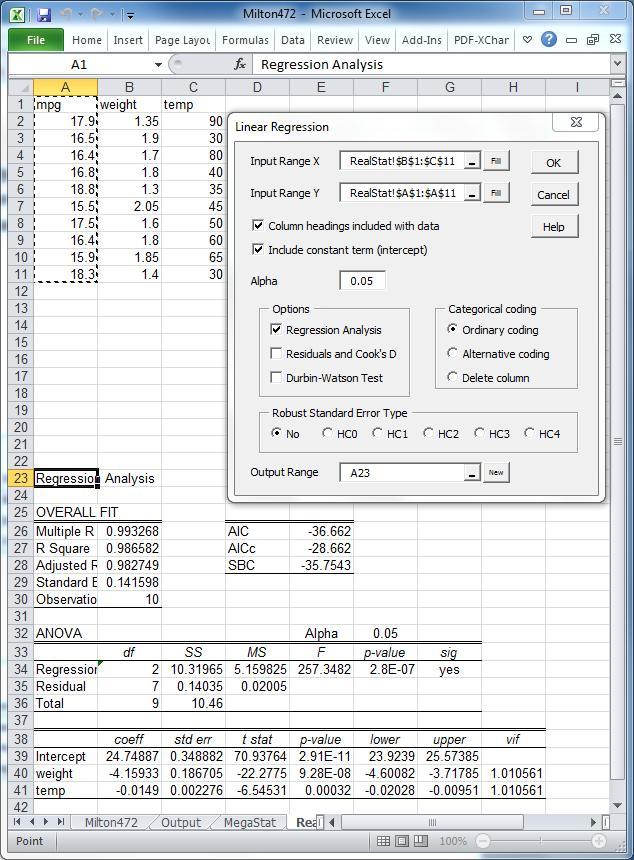
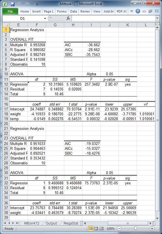
11 Example: Milton/Arnold Examples An equation is to be developed from which we can predict the gasoline mileage of an automobile as a linear function of its weight and temperature at the time of operation. Car No mpg(y) (x 1 /tons) (x 2 / o F) The model specification matrix X, vector of parameter estimates b, and vector of responses y are: X = , b = b 0 b 1 b 2, y = We wish to solve the normal equations X y = X Xb by calculating b = (X X) 1 X y. To this end, note that X y = =

12 Furthermore, X X = = with inverse matrix (X X) 1 = The vector of parameter estimates is b = (X X) 1 X y = = The estimated model is Y = X X 2 + ɛ. Based on this equation, we estimate the mileage of a car weighing 1.5 tons on a 70 o F day to be ŷ = = 17.47mpg. 171

13 The ANOVA F-test for Multiple Regression In simple linear regression the F test from the ANOVA table is equivalent to the twosided test of the hypothesis that the slope of the regression line is 0. For multiple regression there is a corresponding ANOVA F test, but it tests the hypothesis that all regression coefficients (except the intercept β 0 ) are 0. The ANOVA table for multiple regression is Source Sum of Squares DF Mean Square F Ratio Regression Error Total (ŷi ȳ) 2 k SSR/DFR MSR/MSE (yi ŷ i ) 2 n (k+1) SSE/DFE (yi ȳ) 2 n 1 SST/DFT The ratio MSR MSE against is an F statistic for testing H 0 : β 1 = β 2 = = β k = 0 H 1 : Not all β i, i = 1,..., k are zero. Under H 0 : F = MSR MSE F (k, n k 1). 172

14

15 How good is the regression? The mean square error (jäännösvarianssi) SSE (yj MSE = n (k + 1) = ŷ j ) 2 n (k + 1) displayed in the ANOVA table is an unbiased estimator of the variance σ 2 of the population errors ɛ. The square root of MSE is an estimator of the standard deviation σ, usually denoted by s and referred to as the standard error (keskivirhe) of estimate s = MSE. The mean square error and its square root are measures of the size of the errors in regression but give no indication about the explained component of the regression fit. As in the case with only one regressor, we measure the regression fit by R 2 = s2 ŷ s 2 y = SSR SST = 1 SSE SST, the (multiple) coefficient of determination. (Note that again: SST = SSR + SSE.) 174

16 The multiple coefficient of determination R 2 measures the quality of the regression fit as the proportion of the variation in the dependent variable that is explained by the linear combination of the independent variables. Adding new variables to the model can never decrease the amount of variance explained, therefore R 2 will always increase when we add new variables (it will only stay constant if the variables we added are completely useless). For comparing models with varying numbers of regressors it is useful to have a measure of regression fit which decreases under addition of variables of low explanatory power. Such is given by the adjusted multiple coefficient of determination (tarkistettu selitysaste) R 2 = 1 MSE MST = 1 SSE/(n k 1) SST/(n 1), which is related to the ordinary R 2 by R 2 = 1 (1 R 2 n 1 ) n (k + 1). 175

17 Note that the F test for β 1 =... = β k = 0 may just as well be regarded as a test of R 2 = 0, since F = SSR/k SSE/(n k 1) = R2 n (k + 1). 1 R2 k Example: (continued.) MSE = SSE n (k+1) = = 0.02 s = MSE = R 2 = = = R 2 = 1 MSE MST = /9 = Alternatively: R 2 = 1 (1 R 2 n 1 ) n (k + 1) = = F = R2 n (k + 1) 1 R2 k = = The difference to F = in the ANOVA table is due to rounding error. 176

18 Inference in Multiple Regression Properties of the Least-Squares Estimators Now that we learnt how to find the regression parameters (by the method of least squares) and how to assess the usefulness of the regression as a whole (by the ANOVA F test) we would also like to be able to tell for individual regression parameters whether they are statistically significant or not. This requires us to learn something about the sampling distribution of the least square estimator b = (X X) 1 X y for the unknown parameter vector β. For that purpose we define the expected value E(Y) of a vector of random variables Y, that is, Y = (Y 1, Y 2,..., Y n ), as E(Y) = E(Y 1 ) E(Y 2 ). E(Y n ). 177

19 The calculation rules for expectations of random vectors resemble those of scalar expectations: 1. E(C) = C, 2. E(CY) = CE(Y) ( E(Y C ) = E(Y )C ), 3. E(Y + Z) = E(Y) + E(Z); where Y and Z denote (n 1) random vectors and C denotes an (m n) matrix of constants. These rules may be used to show that the least squares estimator b = (X X) 1 X y is an unbiased estimator of β = (β 0, β 1,..., β k ) in the multiple regression model Y = Xβ + ɛ: E(b) = E[(X X) 1 X Y ] = E[(X X) 1 X (Xβ + ɛ)] = E[(X X) 1 X Xβ] + E[(X X) 1 X ɛ)] = (X X) 1 X Xβ + (X X) 1 X E(ɛ) = β. 178

20 Before discussing the variance of b, let us first refresh the definition and some calculation rules for the variance of scalar random variables: 1. V (X) := E[(X E(X)) 2 ] = E(X 2 ) E(X) 2, 2. V (c) = 0 for c constant, 3. V (ax + b) = a 2 V (X) for a, b constants, 4. V (X + Y ) = V (X) + V (Y ) for X and Y independent. If X and Y are not independent, then: V (X + Y ) =E { [(X + Y ) E(X + Y )] 2} =E { [(X E(X)) + (Y E(Y ))] 2} =E[(X E(X)) 2 ] + E[(Y E(Y )) 2 ] + 2E[(X E(X))(Y E(Y ))] =V (X) + V (Y ) + 2E[(X E(X))(Y E(Y ))]. 179

21 Thus, unlike the mean, the variance of a sum of two random variables is, in general, not the sum of the variances. The quantity Cov(X, Y ) := E[(X E(X))(Y E(Y ))] is called the covariance of X and Y. Thus, we obtain the variance of a sum as: V (X + Y ) = V (X) + V (Y ) + 2Cov(X, Y ). From the definition of covariance we obtain the two immediate consequences Cov(X, X) = V (X), Cov(X, Y ) = Cov(Y, X). Furthermore, (X E(X))(Y E(Y )) = XY XE(Y ) Y E(X)+E(X)E(Y ), and hence by taking expectations we see that Cov(X, Y ) = E(XY ) E(X)E(Y ). This implies that Cov(X, Y ) = 0 whenever X and Y are independent, since then E(XY ) = E(X)E(Y ). 180

22 For random vectors it is convenient to collect all covariances between the components of the vector in a single matrix, the so called variance-covariance matrix defined by Var (Y) V (Y 1 ) Cov(Y 1, Y 2 ) Cov(Y 1, Y n ) Cov(Y 1, Y 2 ) V (Y 1 ) Cov(Y 2, Y n ) := Cov(Y 1, Y 3 ) Cov(Y 2, Y 3 ) V (Y 3 ) Cov(Y 3, Y n )......, Cov(Y 1, Y n ) Cov(Y 2, Y n ) V (Y n ) where Y denotes again a vector of random variables Y = (Y 1, Y 2,..., Y n ). Similiar to the calculation rules for variances of scalar random variables we have the following important matrix rule for variance: Var (CY + d) = CVar (Y)C where Y is again an (n 1) random vector, C is an (m n) constant matrix, and d an (n 1) constant vector. 181

23 The assumption of the multiple regression model that Y 1, Y 2,..., Y n are independent with common variance σ 2 may now be written as Var (Y) = σ σ σ 2 = σ2 I, where I is the (n n) identity matrix, a matrix of 1 s on the main diagonal and 0 elsewhere. Recall that our least squares estimator b = (X X) 1 X Y is of the form CY with C = (X X) 1 X. We may therefore use the rule Var (CY) = CVar (Y)C, such that Var (b) = Var [(X X) 1 X Y] = (X X) 1 X Var (Y)[(X X) 1 X ], where, using (AB) =B A and (A 1 ) =(A ) 1 : [(X X) 1 X ] = X[(X X) 1 ] = X[(X X) ] 1 = X(X X)

24 Var (b) = (X X) 1 X Var (Y)[(X X) 1 X ] = (X X) 1 X Var (Y)X(X X) 1 = (X X) 1 X σ 2 IX(X X) 1 = σ 2 (X X) 1 (X X)(X X) 1 = σ 2 (X X) 1. Since σ 2 is unknown, we replace it by our usual estimator, the mean square error s 2 = MSE = in order to obtain SSE n (k + 1) ˆ Var (b) = s 2 (X X) 1 as our estimator for the variance covariance matrix of the least square parameter estimates b = (b 0, b 1,..., b k ) for the unknown parameter vector β = (β 0, β 1,..., β k ). The diagonal elemements s 2 (X X) 1 ii of Var ˆ(b) are the estimated variances of b 0, b 1,..., b k. Their standard errors are therefore given by SE bi 1 = s (X X) 1 ii = MSE(X X) 1 ii. 183

25 Example: (continued.) We found earlier that MSE=0.02 and (X X) 1 = Our variance estimates for the least squares coefficients b 0, b 1 and b 2 are therefore: ˆ V (b 0 ) = = , ˆ V (b 1 ) = = , ˆ V (b 2 ) = = ; with corresponding standard errors SE b0 = = 0.349, SE b1 = = 0.187, SE b2 = =

26 Inference on Single Regression Parameters Recall that X is normally distributed with parameters µ and σ 2 if its density is of the form f(x) = 1 2πσ 2 e (x µ)2 2σ 2, < x < This is denoted by X N(µ, σ 2 ). We say that a random vector Y = (Y 1,..., Y n ) follows a multinormal distribution N(µ, Σ) if its density is of the form f(y)=(2π) n 2 Σ 1 2 exp [ 1 2 (y µ) Σ 1 (y µ) ] with µ = µ 1 µ 2. µ n, Σ = σ1 2 σ 12 σ 1n σ 21 σ2 2 σ 2n σ n1 σ n2 σn 2 denoting µ i = E(Y i ), σ ij = Cov(Y i, Y j ), and σ 2 i = σ ii = V (Y i ) for i, j = 1,..., n. 185

27 Multinormally distributed random vectors have the following two important properties: 1. Each single component of Y is normally distributed with mean µ i and variance σ 2 i : Y = (Y 1,..., Y n ) N(µ, Σ) Y i N(µ i, σ 2 i ). 2. Any arbitrary linear combination of the components of Y is also normally distributed. In matrix form this is written: Z = AY + c N(Aµ + c, AΣA ), } {{ } E(Z) }{{} Var (Z) where A is any (r n) matrix of constants and c is any (r 1) vector of constants. 186

28 We are now in a position to restate the k- variable regression model in matrix form as: Y = Xβ + ɛ, ɛ N(0, σ 2 I); which implies by property 2 from above that Y N(Xβ, σ 2 I). Our interest is in the sampling distribution of b = (X X) 1 X Y. We know already that E(b) = β and Var (b) = σ 2 (X X) 1. Furthermore, since b is just a linear combination of the components of Y, we have again by property 2: b N(β, σ 2 (X X) 1 ), which implies by property 1: b i N(β i, σ 2 b i ), i = 0, 1,..., k; where σb 2 = V (b j 1 j 1 ) = σ 2 (X X) 1 jj with (X X) 1 jj the j th diagonal element of (X X) 1, and j = i + 1, so the first diagonal element is for b 0, the second diagonal element is for b 1, and so on. 187

29 Standardizing yields z = b i β i σ bi N(0, 1). Because the σ bi are unknown, we substitute σ bi 1 by their estimates SE bi 1 = s (X X) 1 ii = and use instead the t-statistic: MSE(X X) 1 ii. t = b i β i SE bi t(n k 1) under H 0 : β i = β i. Alternatively we may calculate (1 α) confidence intervals for β i as [b i ± tα 2 (n k 1) SE bi ]. In particular, we may test for statistical significance of individual regression parameters by calculating the t-statistics t = b i SE bi t(n k 1) under H 0 : β i = 0 or by checking that b i > tα 2 (n k 1) SE bi. 188

30 Example: (continued.) The t-statistics for the regression parameters β 0 (intercept), β 1 (weight), and β 2 (heat) are: t β0 = b 0 = SE b = 70.9, t β1 = b 1 SE b1 = = 22.3, t β2 = b 2 SE b2 = = 6.5. The degrees of freedom are: df = n (k + 1) = 10 (2 + 1) = 7. By calling T.INV.2T(0.001;7) in Excel or by looking up in a table we find that the 0.1% critical value of a 2-sided t-test with 7 degrees of freedom is 5.408, which is smaller than the absolute value of any of the t-statistics above. All regression parameters are therefore significant at 0.1%. 189

31 Using Multiple Regression for Prediction Confidence Interval on Estimated Mean We shall now find a confidence interval for the mean value of the response variable Y for a specific set of values x 1,..., x k of the predictor variables, which have not necessarily been used in developing the regression equation. Let µ Y x : = E(Y X 1 = x 1, X 2 = x 2,..., X k = x k ) = β 0 + β 1 x 1 + β 2 x β k x k = x 1 (k+1) β (k+1) 1, where x = (1, x 1, x 2,..., x k ), β = (β 0, β 1,..., β k ). An unbiased estimator for µ Y x is ˆµ Y x = b 0 + b 1 x 1 + b 2 x b k x k = x b. The variance of ˆµ Y x is such that Var (ˆµ Y x ) = Var (x b) = x Var (b)x = x σ 2 (X X) 1 x = σ 2 x (X X) 1 x, ˆµ Y x N(x β, σ 2 x (X X) 1 x). 190

32 Standardizing and replacing the unknown σ 2 by its estimator s 2 = MSE = t = ˆµ Y x µ Y x s x (X X) 1 x SSE n (k+1) yields t(n k 1). A (1 α) confidence interval on µ Y x is thus [ ] ˆµ Y x ± tα(n k 1)s x (X X) 1 x. 2 Example: (continued.) We estimated earlier the average gasoline mileage for a car weighing 1.5 tons operated on a 70 o F day as ˆµ Y x = =17.47mpg. The standard error of the estimate was s = MSE = We wish to find a 95% confidence interval on µ Y x at x = (1, 1.5, 70). 191

33 We know from previous work that (X X) 1 = A calculation by hand or calling MMULT in Excel yields for x (X X) 1 x: (1, 1.5, 70) ( ) ( ) = The t critical value with 7 degrees of freedom is 2.365, such that a 95% confidence interval in the average gasoline milage for x 1 = 1.5 and x 2 = 70 is ˆµ Y x ± tα 2 s x (X X) 1 x =17.47 ± =17.47 ± 0.16 We can thus be 95% confident that the average gasoline milage of cars weighing 1.5 tons operated on a 70 o F day lies between and miles per gallon. 192

34 Prediction Interval on Single Response Consider next predicting a single response Y x = µ Y x + ɛ. The scalar product x b is also an unbiased estimator of Y x since E(Y x) = E(µ Y x ) + E(ɛ) = x β. But the variance of Ŷ x is larger than the variance of ˆµ Y x due to the additional variation in ɛ. More specifically: Var (Ŷ x) = Var (ˆµ Y x ) + Var (ɛ) = σ 2 x (X X) 1 x + σ 2 = σ 2 (1 + x (X X) 1 x). That is, Ŷ x N(x β, σ 2 (1 + x (X X) 1 x)). 193

35 A similiar argument as for the confidence interval on the estimated mean yields as a (1 α) prediction interval for an individual response: [ ] Ŷ x ± tα(n k 1)s 1 + x (X X) 1 x. 2 Example: (continued.) A 95% prediction interval for a car weighing 1.5 tons operating on a 70 o F day is [17.47 ± ] =[17.47 ± 0.38] =[17.09, 17.85]. (The corresponding confidence interval for the mean response was [17.31,17.63].) Getting confidence intervals for the mean and individual predictions in excel requires use of the array functions MMULT for matrix multiplication and MINVERSE for calculating the matrix inverse. Before entering an array function you must mark an area exactly as large as the output matrix and finish your command with Ctrl+Shift+Enter. 194

36 Partial F Tests Testing a Subset of Predictor Variables In this section we shall present a test based on the F distribution (and in simple cases the t distribution) in order to test whether a subset of the original predictor variables is sufficient for prediction. Consider the regression model Y = β 0 + β 1 X 1 + β 2 X β k X k + ɛ, We refer to this model as the full model. Assume that we propose to reduce the number of predictor variables by deleting r of them, such that we obtain the reduced model: Y = β 0 + β 1 X 1 + β 2 X β k r X k r + ɛ. We wish to test H 0 : reduced model is appropriate against H 1 : full model is needed. This may be done using a partial F test. 195

37 The method used to test H 0 is rather intuitive. We first find the residual sum of squares for both the full model (SSE F ) and for the reduced model (SSE R ) from the corresponding ANOVA tables. We know that for a given model the residual sum of squares reflects the variation in the response variable not explained by the model. If the predictor variables X k r+1, X k r+2,..., X k are important, then deleting them from our model should result in a significant increase in the unexplained variation in Y. That is, SSE R should become considerably larger than SSE F. The partial F test makes use of this idea. It is given by: F = (SSE R SSE F )/r F (r, n (k+1)) MSE F if the null hypothesis, that the reduced model is appropriate, holds true. We reject on the right tail of the distribution, that is, large values of the partial F statistics are taken as evidence that the full model is needed. 196

38 Example: (continued.) Suppose we want to test whether the weight of the car alone is sufficient to predict the gasoline milage of an automobile. From the ANOVA output for the full model we know: SSE F = 0.14 and MSE F = A glance at the ANOVA table for the reduced model reveals that SSE R = and we consider deleting r = 1 variable from the model. The partial F statistic is therefore: F = (SSE R SSE F )/r MSE F ( )/1 = = Calling F.INV.RT(0.01;1;7) or looking up in a table reveals that F 0.01 (1, 7) = The p-value is F.DIST.RT(42.95;1;7)=0.032%. So we reject the null hypothesis that the weight of the car alone would suffice in predicting the gasoline milage of an automobile. 197

39

40 In the special case that we consider to delete only one variable from the full model (as in the preceding example), the p-value for the partial F test coincides with the p-value for the single coefficient t test for the coefficient we are considering to delete from the full model. Indeed, in the previous example the p-value for the temp coefficient is T.DIST.2T(6.545;7)=0.032%, the same as in the partial F test. So the t tests for significance of individual regression parameters may alternatively be interpreted as partial F tests for reducing the full model by the corresponding regression parameter alone. That is so because the absolute value of the t statistic for each single regression parameter is just the square root of the partial F test for deleting the same parameter ( in the preceding example, differences to the ANOVA output for the full model are due to rounding), and we know already that the square of a t-distributed random variable with ν degrees of freedom is F (1, ν)-distributed. 199

41 Qualitative Independent Variables Recall that the purpose of both ANOVA and regression is to forecast the value of a quantitative variable based on some other variable(s). The diffence between ANOVA and Regression is whether the explanatory variable is qualitative (ANOVA) or quantitative (Regression). We shall next consider incorporating both quantitative and qualitative explanatory variables into a linear model for a quantitative dependent variable. As a start-off point we choose qualitative variabels with only two levels, such as available versus not available. Such a variable is called a dummy variable or indicator variable II A, because it indicates if some condition A holds. It has the value 1 when the condition A holds and the value 0 when the condition does not hold. II A = 1 if condition A holds, 0 if condition A does not hold. 200

42 The use of indicator variables in regression analysis does not require any additional computational routines. We just include the indicator variable as an additional explanatory variable, coded as 1 if the quality of interest is obtained and 0 if it is not obtained. Example: (Azcel, Example 11-3.) A motion picture industry analyst wants to estimate the gross earnings generated by a movie (Y /mio $) as a linear function of production costs (X 1 /mio $) and promotion costs (X 2 /mio $). As a third variable she wants to consider whether the film is based on a book (X 3 = 1) or not (X 3 = 0). The estimated coefficient of for X 3 means that having the movie based on a book increases the movie s gross earnings by an average of $7.166 million. 201

43 Regression Model Summary Model R R Square Adjusted R Square Std. Error of the Estimate a a. Predictors: (Constant), Book, PromotC, ProdCost Model 1 Regression Residual Total ANOVA b Sum of Squares df Mean Square F Sig a a. Predictors: (Constant), Book, PromotC, ProdCost b. Dependent Variable: Earnings Model 1 (Constant) ProdCost PromotC Book a. Dependent Variable: Earnings Coefficients a Unstandardized Standardized Coefficients Coefficients B Std. Error Beta t Sig

44 The p-value of for Book means that we can reject H 0 : β 3 = 0 against H 1 : β 3 0 at a significance level of α = 0.1%. This again implies that we have in fact two different regression models depending upon whether the film is based on a book (X 3 = 1) or not (X 3 = 0). The regression model for films based on a book is Y = X X ɛ = X X 2 + ɛ whereas for films not based on a book it is Y = X X 2 + ɛ. We see that the fact that H 0 : β 3 = 0 was rejected implies that different subsamples of the films are described by different regression models with different intercepts, but identical slope coefficients. 203

45 In general, if the regression model contains k quantitative regressors X 1,..., X k and one dummy variable X k+1, then rejection of H 0 : β k+1 = 0 against H 1 : β k+1 0 implies that there are two parallel regression models for the 2 subsamples corresponding to the value of the indicator variable X k+1 : Y = β 0 + k i=1 β k X k + ɛ for X k+1 = 0, and Y = (β 0 + β k+1 ) + k i=1 β k X k + ɛ for X k+1 = 1. Even though we could in principle go and fit own regression models for each subsample separately, we have good reasons to use the dummy variable approach instead: 1) It allows us to test statistically whether there are indeed two separate models needed. 2) By pooling the data from both groups, we improve the efficiency of our estimators for the common regression parameters β 1,..., β k and σ

46 Qualitative Variables with more than 2 levels Rather than introducing a pseudo-indicator with more than 2 levels, we account for a qualitative variable with r levels by using r 1 indicator (0/1) variables as follows: All indicator variables = 0 indicates the first level, all other r 1 levels are indicated by setting the corresponding indicator variable to 1 and the remaining dummies to 0. Example: (continued.) Suppose the analyst is interested not in whether the movie is based on a book, but rather in the category to which the movie belongs: adventure, drama, or romance. Assume furthermore for simplicity, that the only quantitative regressor is production costs (such that we get a regression line rather than a surface). We may then model the r = 3 subgroups adventure, drama, and romance by r 1 = 2 dummy variables X 2 and X 3 as follows. 205

47 Estimating the model Category: X 2 X 3 Adventure 0 0 Drama 1 0 Romance 0 1 Y = β 0 + β 1 X 1 + β 2 X 2 + β 3 X 3 + ɛ yields 3 estimated regression lines: Ŷ = b 0 + b 1 X 1 for adventure, Ŷ = (b 0 + b 2 ) + b 1 X 1 for drama, Ŷ = (b 0 + b 3 ) + b 1 X 1 for romance. Nonrejection of H 0 : β 2 = 0 would imply that adventure and drama films produce the same earnings, while nonrejection of H 0 : β 3 = 0 would imply that adventure and romance films produce the same earnings (given identical production costs X 1 ). A partial F test could be used to test H 0 : β 2 = β 3 = 0, that is that all three categories produce the same earnings (given identical production costs X 1 ). 206

48 Interactions between Qualitative and Quantitative Variables So far we have assumed that the quantitative variable X 1 effects all levels of the qualitative variables in the same way, that is, all regression lines or surfaces are parallel (identical slope coefficients, only intercepts may differ). This assumption may be tested. In the case of one indicator variable X 2, with 2 levels, an appropriate model is Y = β 0 + β 1 X 1 + β 2 X 2 + β 3 X 1 X 2 + ɛ Estimation of this model yields Ŷ = b 0 + b 1 X 1 for X 2 = 0, Ŷ = b 0 + b 1 X 1 + b 2 + b 3 X 1 = (b 0 +b 2 ) + (b 1 +b 3 )X 1 for X 2 = 1. So we may test equality of slopes by testing H 0 : β 3 = 0 against H 1 : β

49 Dummy Regressions as Simple Contrasts Regressing on dummy variables alone replicates the results of contrasts of the form H 0 : µ Dummy=1 = µ Dummy=0. The slope coefficient of a dummy variable equals then the difference in means x Dummy=1 x Dummy=0 and the p-value of the t-test is the same as that of the corresponding contrast. Example. Consider again the errors made under influence of drug A, drug B, or both drugs. 208

50

51 Polynomial Regression The mathematical framework of multiple regression may be used to model relationships between a response variable Y and a single predictor variable X, where the relationship between X and Y is curved rather than linear. A one-variable polynomial regression model is Y = β 0 + β 1 X + β 2 X β m X m + ɛ, where m is the degree of the polynomial (the highest power of X in the equation), which is also called the order of the model. Polynomial models of order higher than 2 are very rarely used in practice, due to the danger of overfitting, and because the dependence between different powers of X may result in difficulties to find the right regression parameters (so called multicollinearity, to be discussed later). 210

52 Graph 25,0 20,0 Sales 15,0 10,0 R Sq Quadratic =0,959 R Sq Linear = 0,895 5,0 0,0 2,0 4,0 6,0 8,0 10,0 12,0 14,0 Advert

53 Example: (Azcel Example 11 5.) Sales response to advertising usually follows a curve reflecting the diminishing returns to advertising expenditure. As a firm increases its advertsing expenditure, sales increase, but the rate of increase drops continually after a certain point. The preceding slide contains data on sales revenues as a function of advertising expenditure. As is evident from the scatterplot, scales as a function of advertising is better approximated by a polynomial of 2nd order than by a straight line. So we attempt to fit: Y = β 0 + β 1 X + β 2 X 2 + ɛ and obtain (see next slide): Ŷ = X X 2. (Note that the regression model is not fully satisfactory as it is evident from the residual plot that there is left some autocorrelation in the residuals.) 212

54 Linear Regression Results Model: Linear_Regression_Model Dependent Variable: Sales Sales Number of Observations Read 21 Number of Observations Used 21 Source Analysis of Variance DF Sum of Squares Mean Square F Value Pr > F Model <.0001 Error Corrected Total Root MSE R-Square Dependent Mean Adj R-Sq Coeff Var Variable Label DF Parameter Estimates Parameter Estimate Standard Error t Value Pr > t Intercept Intercept Advert Advert <.0001 AdvSQR AdvSQR <.0001