Lecture 1: Introduction to Regression Discontinuity Designs in Economics

Transcription

1 Lecture 1: Introduction to Regression Discontinuity Designs in Economics Thomas Lemieux, UBC Spring Course in Labor Econometrics University of Coimbra, March

2 Plan of the three lectures on regression discontinuity designs! Lecture 1: " Introduction to regression discontinuity (RD) designs " RD designs as local randomized experiments and the manipulation problem! Lecture 2: " RD designs: A User Guide! Lecture 3: " Recent Advances and Applications! The main reference for the lectures is D.S. Lee and T. Lemieux Regression Discontinuity Designs in Economics Journal of Economic Literature, June 2010

3 Introduction to RD Designs! Before introducing any formalities and telling you exactly what a RD design means, I will work through a motivating example.! RD Designs were first introduced by Thistlethwaite and Campbell fifty years ago ( RD Analysis: An Alternative to Ex Post Fact Experiments, Journal of Education Psychology, 1960). " The application they consider is merit awards given in recognition of good academic performance (university grades above a certain cutoff GPS) " They use the RD design to see whether these merit awards have an (psychological) impact on future academic achievement, e.g. on the decision to go to graduate school.! I will work through a related example from a recent paper by Mark Hoekstra ( The Effect of Attending the Flagship State University on Earnings: A Discontinuity-Based Approach, Review of Economics and Statistics, November 2009, pp )

4 Selection problem in schooling! A large number of studies have shown that graduates from more selective programs or schools earn more than others " Medecine, science, economics? " MBAs from HBS earn more than others! Lead to sometimes extreme competition in some countries " Grandes écoles in France " University of Tokyo in Japan! But it is difficult to know whether the positive earnings premium is due to " a true causal impact of human capital acquired in the academic program, or " a spurious correlation linked to the fact that good students selected in these programs would have earned more no matter what! The latter point can either reflect a signalling effect, or a straight selection effect: " Famous Harvard dropouts (Bill Gates and Mark Zuckerberg): consistent with selection but not necessarily with signalling

5 RD: solution to the selection problem! Untangling the causal and selection effects is a difficult challenge! Lots have been written about this in econometrics and labour economics, but in many cases suggested methods (e.g. IV) are not applicable or not very convincing! A great way to answer that question would be to run an experiment: " Take BC students applying both to UBC (Vancouver) and UBCO (Kelowna) " Instead of admitting them the regular way, just flip a coin to decide whether they get into UBC or UBCO " Follow them up 10 years later to see whether those admitted to UBC earn more than those admitted to UBCO.! Great idea, but nobody will let me run that experiment! But say that the entry cutoff is a high school GPA of 88 percent at UBC. " They would perhaps let me flip a coin for those with GPAs of 87 or 88 percent " RD strategy: but since the 87s and 88s are essentially identical, I can do as well as in a randomized experiment by tracking down the long term outcomes for the 88s (admitted to UBC) and the 87s (admitted at UBCO) :

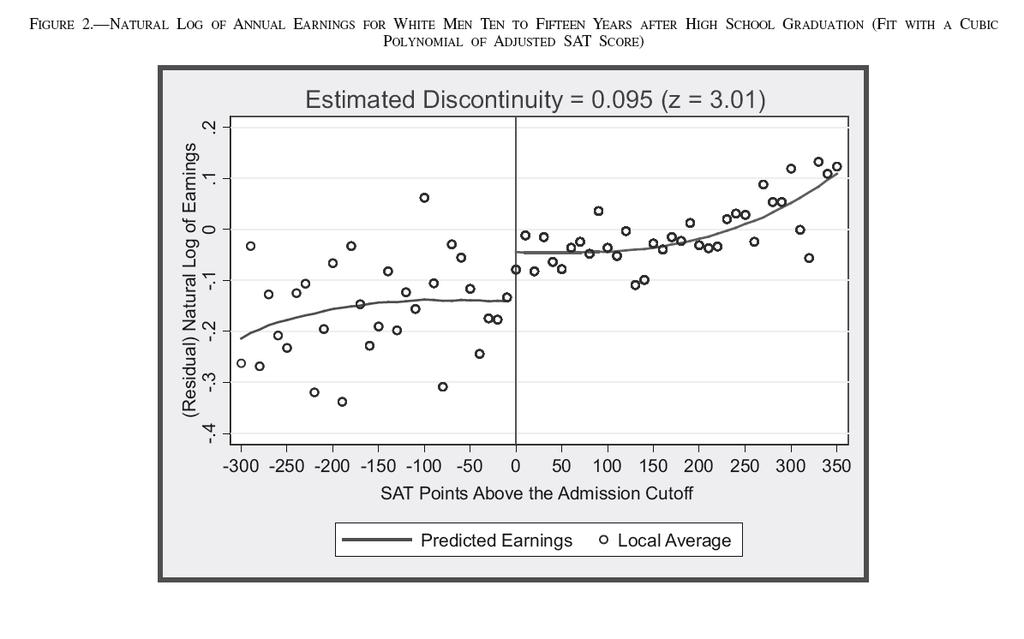
6 Hoekstra paper! Where there is a cutoff there is a RD! Fortunately, it is typical for selective schools and programs to use fairly strict grade cutoffs for admission! In the United States, most schools used SAT (or ACT) scores in their admission process! For example, the flagship state university considered here uses a strict cutoff based on SAT score and high school GPA! For the sake of simplicity, let s just focus on the SAT score (adjusted depending on GPA)! Hoekstra is then able to match (using social security numbers) students applying to the flagship university in to their administrative earnings data for 1998 to 2005! As in any good RD study, pictures tell it all, so let s just focus on those

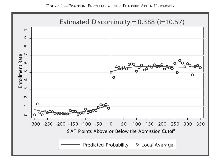
7 Enrollment data

8

9 A few comments! The graphs show what we mean by a RD design: " The smooth relationship between earnings and SAT score likely reflects the fact that more able students are also more productive workers " But it is hard to think of any reason for the discontinuity besides the cutoff rule in admission " So the discontinuity is what enables us to estimate the causal effect! This is a example of what is called a fuzzy: RD design: " Sharp RD design: Nobody below the cutoff gets the treatment, everybody above the cutoff gets it " Fuzzy RD design: The probability of getting the treatment jumps discontinuously at the cutoff, but it needs not jump from 0 to 1! To get the causal effect in a fuzzy RD design, we need to adjust the effect on earnings (0.095) by the fraction of people induced to go the flagship university (0.388). Implies a very large effect of (0.095/0.388) or about 28 percent.! SAT score is what we will later call the assignment variable (sometimes called forcing or running variable)

10 RD designs: a brief history of thought! What do we mean by a design?! Internal vs. external validity! Formal modelling: " The intuitive regression approach " Hahn, Todd and van der Klaauw (HTV, Econometrica 2001): the potential outcomes approach " Lee (Journal of Econometrics, 2008): RD designs as a localised randomized experiment! Threat to validity: " The manipulation problem

11 RD as a research design! According to Wikipedia Research designs are concerned with turning the research question into a testing project! Not a traditional way of thinking about research in economics, but very common in medical science, for example (randomized controlled trials, etc.)! Provides a useful way of thinking about the broader identification strategy and the narrower estimation methods as two separate things " Research design/identification strategy: RD, randomized experiments, natural experiments, non-experimental methods " Estimation methods: IV, difference-in-differences, matching, local linear regressions (in RD designs), etc.! If you have a RD research design for the problem at hand, you can then implement it using a variety of tools we will talk about in the next lecture

12 Internal vs. external validity! Internal validity: " According to Brewer (Research Design and Issues of Validity, 2000) Inferences are said to possess internal validity if a causal relation between two variables is properly demonstrated " We think that RD design have typically a high level of internal validity because they provide a convincing way of estimating a causal effect! External validity: " Brewer: Inferences about cause-effect relationships based on a specific scientific study are said to possess external validity if they may be generalized from the unique and idiosyncratic settings, procedures and participants to other populations and conditions " Problematic for randomized experiment (Heckman, Deaton, etc.) " Even more problematic for RD design as we only identify a causal effect for agents right at the cutoff point

13 Thistlethwaite and Campbell: simple regression approach Regression: Y i = D i! + X i " + # i X i : assignment variable D i : treatment variable, D i =1[X i!c] General problem in such a regression: # i and D i are potentially correlated RD solution: D i only depends on X i (D i =1[X i!c]), so # i and D i cannot be correlated once we have controlled for X i (in a smooth way)

14 Figure 1: Simple Linear RD Setup 4 3 Outcome variable (Y) 2! 1 0 C Assignment variable (X)

15 HTV: The potential outcomes approach «Potential Outcomes» Y = Y(1) when D =1 Y = Y(0) when D =0 E[Y(1) - Y(0)] (the average treatment effect or ATE) Hahn, Todd et van der Klauuw (2001): The TE at X=c! = E(Y(1)-Y(0) X=c) is identified under the assumption that the functions E(Y(1) X) et E(Y(0) X) are continuous. HTV suggest estimating! using local linear regressions (LLR)

16 Figure 2: Potential outcomes approach Observed 3.00 Outcome variable (Y) E[Y(1) X] Observed B A E[Y(0) X] Xd Assignment variable (X)

17 Lee (2008): local randomization! Randomization: experimental approach (in laboratory or field setting) => comparison of means! While RD is a non-experimental design, we have local randomization provides that the following assumption holds (Lee, 2008):! Assumption: agents have imperfect control over X. For instance, you can study harder to do well in a test, but there is always some randomness left in the result " Intuition: the randomness guarantees that the potential outcome curves are smooth (e.g continuous) around the cutoff point! It is then possible to test whether this assumption holds as in the case of a randomized experiment: " Should not be any difference between predetermined covariates on each side of the cutoff point («balanced covariates») " The density of X should be continuous at the cutoff point c (McCrary 2008)

18 Figure 3: Randomized Experiment as a RD Design E[Y(1) X] Observed (treatment) 3.0 Outcome variable (Y) Observed (control) E[Y(0) X] Assignment variable (random number, X)

19 Threat to (internal) validity: manipulation problem! Key assumption in Lee (2008) is that agents have imperfect control over the assignment variable! A test score is a good example of such a variable, but potential problems can arise if we have " Cheating (to get just right above the cutoff) " Instructor moves up student a few points below the passing grade to exactly the passing grade " Students who fail are allowed to retake the test! In all cases, the result is that people just to the left and just to the right of the cutoff are no longer comparable! The manipulation problem is potentially more severe in cases where agents have more direct control over the assignment variable " Example: numbers of weeks/hours to qualify for UI.

20

21 Testing for manipulation! Important advantage of RD over many other approaches (including IV) is that the key identifying assumption (no manipulation) is testable! Balanced covariates: " We only need to include the treatment variable (D) and the assignment variable (X) in the regression model. Gives us the freedom to see whether other covariates (e.g. family background) evolve smoothly around the cutoff point " Similar to randomized experiments in this regard! Continuous density: " If instructor moves up students with a 48 or 49 percent grade to 50 percent, we will see in the data an abnormal concentration of students at 50 percent

22 Lecture 2: A User Guide to RD Thomas Lemieux, UBC Spring Course in Labor Econometrics University of Coimbra, March

23 Step-by-step approach using Lee s voting application as an example! Graphing the raw data " Treatment and outcome graphs " Density of the assignment variable! Estimating the regression " Polynomial models " Local linear regressions and choice of bandwidth! Testing the validity of the RD design " Discontinuity in the density " Testing whether covariates are balanced! Should we include covariates?! Checklist

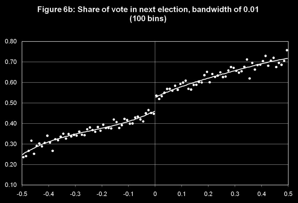
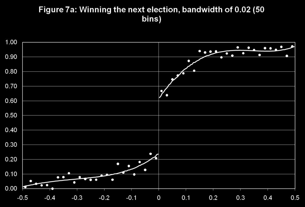
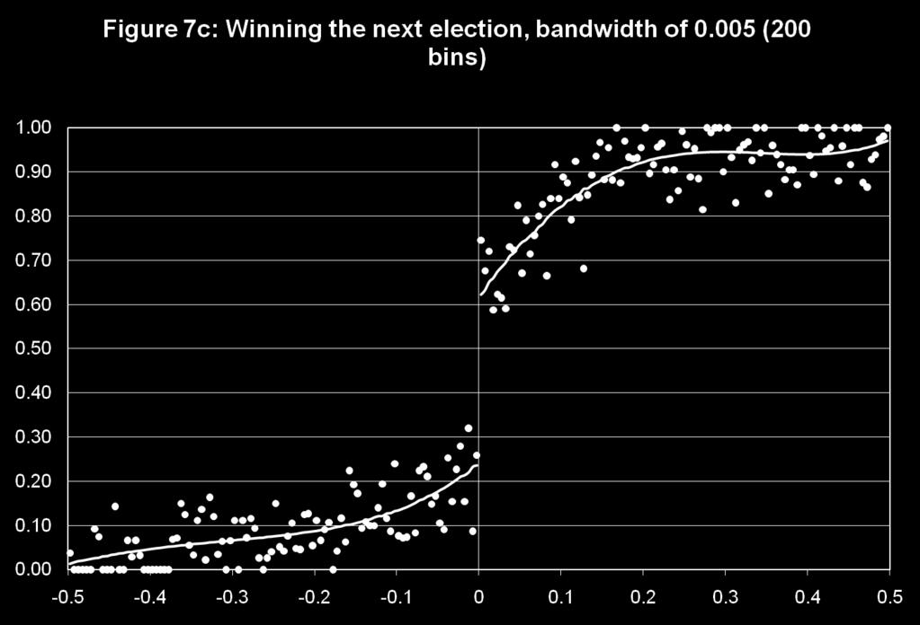
24 Voting example! Voting and election rules a fertile ground for using RD designs! Lee (2008) uses data from elections at the US House of Representatives to look at incumbency effects! Most (80-90 percent) representatives get re-elected two years later. Could either reflect heterogeneity (good politicians get re-elected) or a causal effect of incumbency (fund raising, etc.)! Can sort this out by looking at close elections: probability that a democrat gets elected depending on whether he/she narrowly won or narrowly lost the election two years ago! RD design ( first stage or treatment graph is trivial)

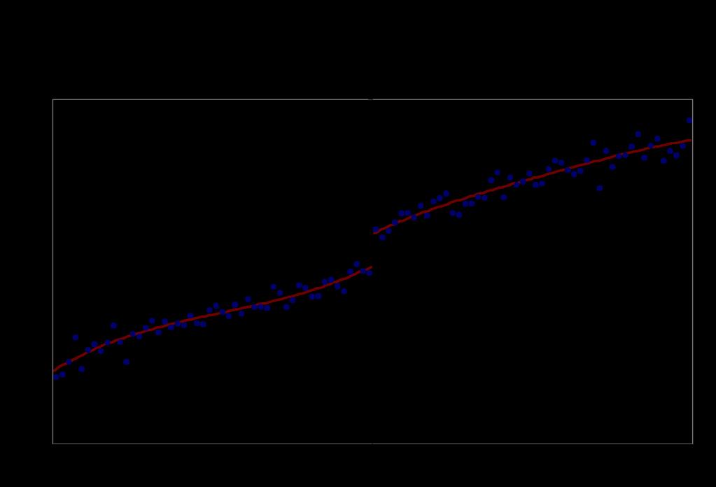
25 Treatment and outcome graph! These are the two core graphs in a RD study " Treatment (D) graph indicates the cutoff rule binds in practice (sometimes trivial) " Outcome (Y) graph is the most convincing evidence for whether or not there is a treatment effect! Suggestion is to show both the raw data (typically mean of D or Y in a small bin) and smoothed data (e.g. cubic or quartic function in X)! Bin means (k=1,..k) are computed as follows:! Choice of binwidth (h=b k+1 - b k ) is an issue: " Too narrow we get very noisy data and don t see much " Too wide we can oversmooth the raw data and fail to see what happens right at the cutoff " In addition to the eyeball estimator we suggest more formal procedures such as cross-validation in the JEL paper

26

27

28

29

30

31

32 Density of the assignment variable! Consider the number of observations in each bin k! An abnormal concentration of observations right at the cutoff point suggests there may be a manipulation problem! A usual way of visually looking at this is to either show the " Histogram: plot N k /N " Density: plot N k /(Nh), where h=b k+1 - b k! As we will later see, one can formally test for manipulation by looking at whether there is discontinuity in the density at the cutoff " Run regression of N k /(Nh) on X on each side of the cutoff and test whether there is a significant jump at the cutoff

33

34 Estimating the regressions! This is the key part of the empirical analysis " Provides regression estimates of the treatment effect! Two most popular methods consists of either fitting " flexible polynomial regressions over a relatively wide range of data ( parametric estimates ) " Local linear regressions (LLR) in a narrow range around the cutoff ( nonparametric approach )! Both approaches are defendable though LLRs are closer in spirit to the RD concept where we should focus on what happens right at the cutoff! In practice, varying the range of the estimation (the bandwidth) and the order of the polynomial is a good way of assessing the robustness of the results! The two approaches are, thus, complementary

35 Estimating the regressions! Highly advisable to run separate regressions (different slopes) on each side of the cutoff! Otherwise we are constraining the treatment effect to be a constant function of X (see potential outcomes graph)! The most convenient way of implementing this in practice is to run a pooled regression with interactions between D and X as it provides a direct estimate of the treatment effect (estimated effect of D) and its standard error! For a linear specification the regression is:! Where we first subtract c from X so that! gives us the effect of D when X=c (X-c=0), ie the treatment effect at the cutoff

36 Polynomial regressions! We simply increase the order of the polynomial in X starting with the linear regression! For example, for a third order polynomial just estimate:! Procedure such as AIC can then be used to more formally select the order of the polynomial. Nothing special about RD here relative to other searches for adequate specification in regression analysis.

37 Local linear regressions (LLR)! Estimate linear regression in the neighbour hood of the cutoff " Estimate the model for c-h! X! c+h, where h is the bandwidth! The approach is non-parametric because we promise that we will choose a smaller and smaller value of h as the number of observations increases " This is a good idea as we ideally like to use data as close as possible to the cutoff " But having h 0 as N " is a bit of an empty promise, as we only have one data set with a fixed N " So even though this is a non-parametric approach, from a practical point of view this just amounts to running standard regressions! A more important question from a practical point of view is how to choose h in our one data set with a given N? " Rule 1: try different values to see how robust the results are " Rule 2: try formal procedures such as rule-of-thumb or cross-validation

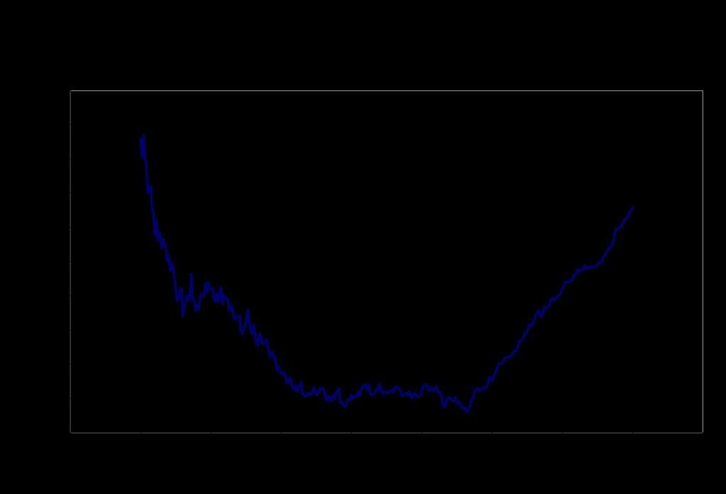
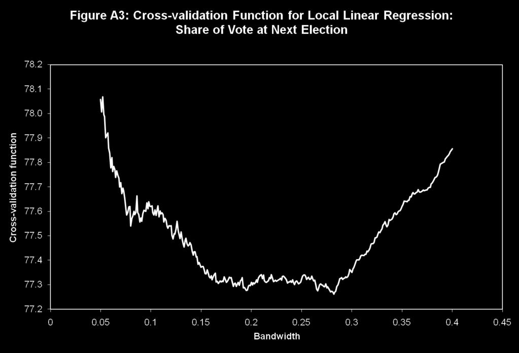
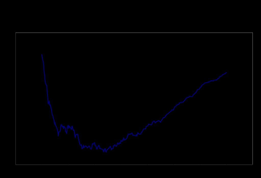
38 Bandwidth choice: cross validation! Well known tradeoff in the choice of h: " We lose efficiency (precision) when h gets smaller " But the bias (if the underlying regression is not linear) increases when h gets larger! Optimal bandwidth is the one that minimizes the mean square error (variance plus bias squared)! Problem in practice is that we don t know what the true functional (and thus the bias) is.! Cross validation procedure: " For observations i on the left (X<c), run a linear regression with observations within a window h to the left of X i, and compute the predicted value of Y using this regression. " Do the opposite for observations on the right hand side of c " The mean square error is the average of the square of the prediction errors

39 Cross validation! Formally, the cross validation criterion is defined as! We just pick the value of h that minimizes the cross validation criterion by doing a grid search! Econometricians have suggested other procedures for choosing the bandwidth. See, e.g. Imbens and Kalyanaraman (2009)! For the voting example, the optimal bandwidth (CV) is for the share of vote, and for the probability of winning the next election. Pretty wide bandwidths...

40

41

42 Regression results! Table 2a: Share of votes! Table 2b: Probability of winning! Figure B1: A graphical illustration of the robustness of the results

43

44

45

46

47

48 Testing for manipulation! Important advantage of RD over many other approaches (including IV) is that the key identifying assumption (no manipulation) is testable! Balanced covariates: " Use covariates W instead of the outcome variable Y on the left hand side of the regressions. If the RD design is valid, we should not find a discontinuity in W since agents just to the left and just to the right of the cutoff should be very similar " Similar to randomized experiments where we first test whether baseline covariates are the same for the treatment and control groups. Systematic differences suggest that randomization failed! Continuous density: " One we have computed the density in each bin, we can once again run the regressions using the density (as opposed to Y) as the left hand side variable and see whether there is a significant jump at the cutoff

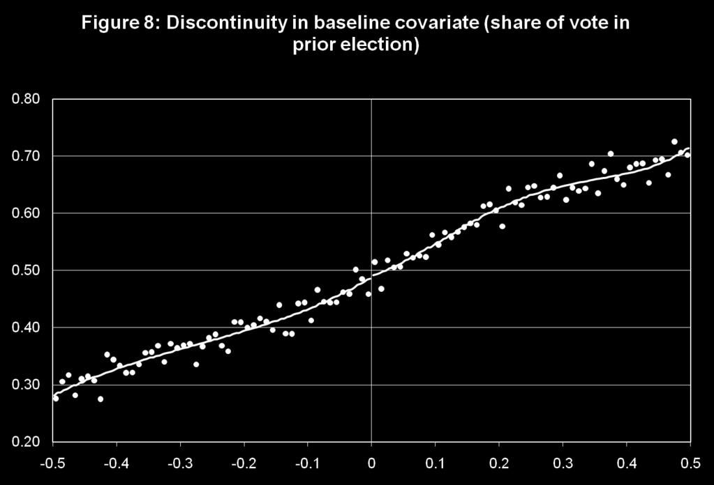
49

50

51 Should we include covariates?! When the RD design is valid, other covariates (e.g. family background in Hoekstra) should be similar on both sides of the cutoff! Orthogonal to the treatment dummy D conditional on X! No bias linked to the exclusion of covariates! But including the covariates (W) may reduce the estimation noise Y i = D i! + X i " + W i # + $ i! When W is not included in the regression, the error is W i # + $ i instead of $ i which results in a higher residual variance and less precise estimates of the treatment effect! Same argument as with randomized experiments! But if your results change a lot when you include the covariates you should be worried. Likely reflects an imbalance in the covariates.

52 Lee and Lemieux s checklist 1. To assess the possibility of manipulation of the assignment variable, show its distribution 2. Present the main RD graph using binned local averages 3. Graph a benchmark polynomial specification 4. Explore the sensitivity of the results to a range of bandwidths, and a range of orders to the polynomial 5. Conduct a parallel RD analysis on the baseline covariates 6. Explore the sensitivity of the results to the inclusion of baseline covariates

53 Implementation in Stata: Lee data set! The data set used in Lee and Lemieux (2010) is available at Key variables are " margin: margin of victory, the assignment variable " treat: dummy variable for where a Democrat got elected (margin>0). This is the treatment variable " share: first outcome variable, the winning share in the next election. " win: second outcome variable, dummy for whether a Democrat got elected in the next election! One can the running simple regression. For instance, to estimate a local linear regression for share with a bandwidth of 0.1, just do: use leedata.dta gen tmargin=treat*margin reg share treat margin tmargin if margin>=-.1 & margin<.1 Output on the next slide

54 . use leedata.dta. gen tmargin=treat*margin. reg share treat margin tmargin if margin>=-.1 & margin<.1 Source SS df MS Number of obs = F( 3, 1205) = Model Prob > F = Residual R-squared = Adj R-squared = Total Root MSE = share Coef. Std. Err. t P> t [95% Conf. Interval] treat margin tmargin _cons

55 Guido Imbens stata software! Available at along with an artificial data set for practice! Description of the software at: 09aug4.pdf! Provides an automatic way of selecting the optimal bandwidth for local linear regressions for both the sharp and fuzzy RD design! Main stata command is rdod.ado! Example of program (rd_log_09aug4.do) on the next slide

56 /* example of fuzzy regression discontinuity design */ /* read in data */ infile y w x z1 z2 z3 using art_fuzzy_rd.txt, clear /* display summary statistics */ summ /* estimate rd effect */ /* y is outcome */ /* x is forcing variable */ /* z1, z2, z3 are additional covariates */ /* w is treatment indicator */ /* c(0.5) implies that threshold is 0.5 */ rdob y x z1 z2 z3, c(0.5) fuzzy(w) /* if details on estimation are required */ rdob y x z1 z2 z3, c(0.5) fuzzy(w) detail

57 Lecture 3: Miscellaneous topics in RD designs Thomas Lemieux, UBC Spring Course in Labor Econometrics University of Coimbra, March

58 Plan for the lecture! Fuzzy RD design " Connection with TSLS " Fuzzy RD, LATE, and general interpretation issues! Discrete assignment variable! An incomplete survey of recent applications " Lots of them " Fields of application " Types of cutoffs! Two examples from labour! Questions and discussion

59 Fuzzy RD design! Here there is a discontinuity in the probability of treatment at the cutoff, but unlike the case of the sharp RD it does not go up from 0 to 1! It is useful to introduce a new dummy variable T i =1[X i!c], which simply indicates whether the assignment variable has crossed the cutoff point! In the sharp RD design we have D=T, but not here! One can think of T as an instrumental variable for D in a regression model for Y on X and D! The influential Angrist and Lavy paper on Maimonides rule (QJE 1999) was actually a fuzzy RD study (cutoff at 40 pupils for school classes) but they presented it as an IV study

60 Fuzzy RD: Basic setup! Two equations model (f(.) and g(.) are flexible functions)! We can also write the reduced form:! The parameter! r ="! can be interpreted as an intent to treat (ITT) effect! Very similar to a standard IV setup

61 Fuzzy RD: Estimation! One could either: " Estimate the two reduced forms in X and T and compute the treatment effect! as the ratio of! r over " " Run TSLS using T as an instrument for D! Advisable to use the same specification for f(.) and g(.). " Polynomial model: use the same order of polynomial " LLR: use the same bandwidth. The one for the Y equation is the most natural one to use (we expect the bandwidth for D to be quite wide)! An advantage of TSLS is that it provides a simple way of obtaining the standard errors! Exactly identified model (by design, one instrument T for one endogenous regressor D)! But weak first stage problem may occur if the jump in the probability of D=1 at c is small.

62 Fuzzy RD: interpretation! In the model we wrote we implicitly assume that we have a constant treatment effect!! But if the treatment effect is heterogenous we have a similar interpretation problem as in an IV setting: " Under the assumption of monotonicity (Imbens and Angrist, 1994) we can identify a local average treatment effect (LATE) among those induced to treatment (compliers)! Even narrower here since we only get the LATE for people at X=c! But things are not as bad as they seem since agents at the cutoff come with various values of observable (W) and unobservable (u) characteristics. " It can be shown in the sharp RD case (bit more complicated in fuzzy RD) that the estimated treatment effect is the following weighted average

63 Discrete assignment variable! When the assignment variable is discrete we can no longer go as close as possible to the cutoff.! The role of the regression is now (in part) to extrapolate to the cutoff! Not as clean as in the case with a continuous X, but unless X is very coarse not much problems arise in most empirical applications! Since we now have a grouping structure, it is important to correct standard errors by clustering on X.! Natural goodness-of-fit test of the regression model based on the square deviation between the regression line and the average value of Y for each (discrete) value of X

64 Applications! RD not used much in economics until the late 1990s.! But hundreds of studies since then, starting with Van der Klaauw (IER, 2002)! We provide a partial survey in the JEL piece that would have been many times larger had we included working papers! Few people (in my opinion) could have predicted only 10 years ago the sheer volume of recent research based on RD designs! Two possible explanations: " Cutoff rules are very wide spread " Much more data available now, especially administrative data sets! An important advantage of RD designs is that they are well suited to large administrative data sets with " Few covariates " Lots of observations and all the relevant information about cutoffs and assignment variables since those have to be used in the administration of programs

65 Main fields of applications! In Table 4 of the JEL paper, we summarize 77 recent RD studies. The distribution across fields is as follows: " Education: 26 " Labour markets: 18 " Political economy: 8 " Health: 7 " Crime: 5 " Environment 4: " Others: 11! Example of cutoffs include " Age: 21 for drinking, 65 for US medicare, 18 for young offenders, 25 for the British New Deal (employment programs), 30 for welfare in Quebec, etc. " Pollution levels (non-attainment cutoff) " Weeks or years of work (UI, pension eligibility, etc.) " Geographical (school boundaries, UI regions)

66 Examples of recent applications in labour! Lemieux and Milligan (2008): Age 30 cutoff for social assistance in Quebec until the late 1980s! Lalive (2008): UI in Austria. Lots of cutoffs, both geographical and age based.

67 Lemieux and Milligan, 2008! Social assistance (SA) in Québec! During the 1980s, SA benefits were much lower for adults with no dependent children under the age of 30 than for those age 30 and above.! Data from the Canadian Census! Focus on male high school dropouts

68 Figure 1: Social Assistance Benefits, Single Employable Individual (benefits in constant 1986 dollars) Monthly benefits (1986 $) Under and over

69 Employment rate in 1986 (reference week) Employment rate Age (census day)

70 Regression results Empl. rate Empl. Rate Difference Weekly Specification for age last year at census in empl. rate hours Mean of the dependent variable Regression discontinuity estimates Linear *** *** ** ** (0.012) (0.012) (0.011) (0.54) Quadratic *** *** ** ** (0.013) (0.012) (0.012) (0.61) Cubic ** *** ** * (0.018) (0.014) (0.013) (0.70) Linear spline *** *** ** *** (0.013) (0.011) (0.013) (0.55) Quadratic spline ** * (0.024) (0.018) (0.016) (0.94) Goodness of fit statistic (p-value) Linear Linear spline

71 Employment rate for the whole population of men (1/5 in the long form census) 0.95 Employment rate (census week) Age Quebec 86 Quebec 91 ROC 86 ROC91

72 Lalive, Journal of Econometrics 2008! Incentive effect of the maximum duration of unemployment insurance in Austria! In June 1988, maximum duration went up from 30 to 209 weeks for individuals age 50 and above living in certain regions of the country! Linked to the collapse of the steel industry, which was concentrated in some regions of the country

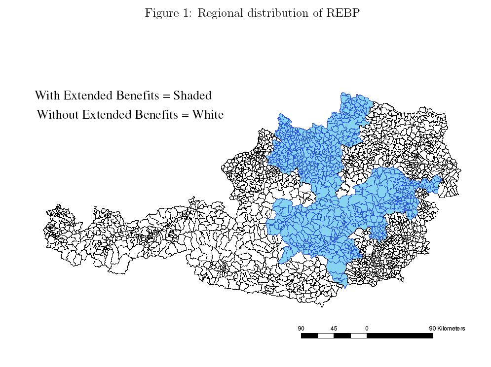
73

74

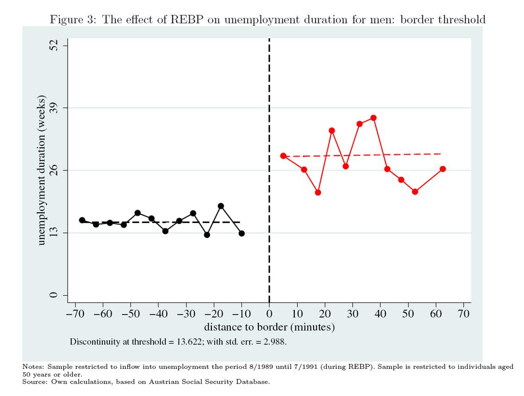
75