Efficient Fluid-Solid Coupling Algorithm for Single-Phase Flows

Transcription

1 Efficient Fluid-Solid Coupling Algorithm for Single-Phase Flows Yen Ting Ng Chohong Min Frédéric Gibou April 11, 009 Abstract We present a simple and efficient fluid/solid coupling algorithm in two-spatial dimensions. In particular, we consider the numerical approximation of the Navier-Stokes equations on irregular domains and propose a novel approach for solving the projection step with Neumann boundary conditions on arbitrary shaped objects. This method is straightforward to implement and leads to a symmetric positive definite linear system for both the Projection step and for the implicit treatment of the viscosity. Both the density and the viscosity can be varying in space, which can serve as a basis for two-phase flows simulations. We demonstrate the accuracy of our method in in the L 1 and L norms. We apply this method to the simulation of a flow past a cylinder and show that our method can reproduce the known stable and unstable regimes as well as correct lift and drag forces. We also apply this algorithm to the coupling of flows with moving rigid bodies. 1 Introduction The Navier-Stokes equations are the fundamental equations of fluid dynamics with countless applications, from engineering to biology. Oftentimes, the coupling between fluids and solids is necessary, for example in micro-fluidics or porous media flows, where the interaction between the fluid and the solid is specific to the physical characteristics of the solid, e.g. through the definition of the so-called contact angle, which in turns requires the accurate computation of the fluid velocity adjacent to the solids boundary. It is therefore important to develop a numerical method that is also convergent near the objects boundary. We note that the notion of contact angles only makes sense in the context of two-phase flows and might involve other issues than the accurate solution of the fluid velocity near the objects boundary, but it emphasizes that an accurate Navier-Stokes solver for irregular domains will serve as a building block for applications beyond single phase flows. The projection method, introduced by Chorin [3] is a very efficient method to solve the Navier- Stokes equations. Its ease of implementation on regular domains is based on the fact that the discretization of the Poisson equation can be decoupled in each of the Cartesian directions, so that imposing the necessary Neumann boundary condition is straightforward. The difficulty in using Computer Science Department, University of California, Santa Barbara, CA Mathematics Department and Research Institute for Basic Sciences, KyungHee University, Seoul, Korea Mechanical Engineering Department & Computer Science Department, University of California, Santa Barbara, CA

2 a projection method on irregular domains is thus primarily to impose the Neumann boundary condition when the contour of the solid objects is not necessarily aligned with the Cartesian grids. Several approaches such as the immersed boundary method of Peskin [14], the immersed interface method Leveque and Li [9] and the ALE method of Hirt [8] have been proposed to represent the boundary of an object and simulate its influence on the fluid dynamics, often with the side-effects of being more computationally expensive (due to non-symmetric linear systems), the loss of accuracy near the solids boundary since considering a smeared out interface, or being more challenging to implement. Because of the lack of a simple method that can accurately solve this problem, one often opts for describing the solids boundary by rasterization, i.e. the objects share are approximated by forcing their boundary to follow the grid lines. This approach is obviously straightforward to implement, but it produces solutions that do not converge in the L norm and show staircase effects near the walls; only the average velocity field is convergent. The loss of accuracy can in turn be problematic, for example in imposing a contact angle condition, since it requires the value of the fluid velocity in the region where it is not computed accurately. In [], Batty et al. presented a methodology based on energy minimization to account for the fluid-solid coupling. This method is able to reproduced the average fluid dynamics and considers boundary that are not necessarily aligned with the grid lines. However, as we show in section 4, this method is not convergent in the L norm with large O(1) errors near the solids boundary. In this paper, we present a novel projection method that is straightforward to implement, produces a symmetric positive definite linear system and is second-order accurate in both the L 1 and L norms. Standard Projection Method The incompressible Navier-Stokes equations describe the motion of fluids and are written as: ρ(u t + (U )U) = p + [µ( U + ( U) T )] + ρf, U = 0, where t is time, ρ the fluid s density, U =< u, v, w > the velocity field, p the pressure, µ the viscosity and F the forcing term, such as the gravity field. The seminal work of Chorin [3] described a method to solve the Navier-Stokes equations based on the Hodge decomposition, which states that any vector field U can be decomposed into the sum of a divergence-free vector field U and a weighted gradient field p ρ for some scalar function p and some known positive function ρ. The projection method consists of three stages: First, given the velocity field U n at time t n, an intermediate velocity U is calculated for a time step t by ignoring the pressure component, e.g.: U U n t + U n U n = 1 ρ n [µn ( U n + ( U n ) T )] + F, then the velocity fluid U n+1 at the new time step t n+1 is defined as a projection of U onto the divergence free vector space: U n+1 = U t pn+1 ρ n+1.

3 Figure 1: Standard MAC grid configuration: The pressure is sampled at the cells center (circles), the x-component of the velocity field is sampled on the vertical faces (rectangles), and the y- component of the velocity field is sampled on the horizontal faces (triangles). The irregular domain is represented by the shaded area. The incompressibility condition U n+1 = 0 for the new fluid velocity is enforced by choosing the (scalar function) pressure p n+1 to satisfy the Poisson equation: ( ) p n+1 ρ n+1 = U, (1) t with Neumann boundary conditions on the domain s boundaries and on the solid objects. ( ) p n = n (U bc U bc ). ρ 3 A Novel Hodge Decomposition on Irregular Domains In the case of an irregular domain, it is not obvious how to choose a scalar function p that will enforce the divergence free condition. The reason is due to the fact that it is not straightforward to solve the Poisson equation with Neumann boundary conditions at the boundary of an irregular domain, especially if one seeks to design a simple methodology that can be applied dimension by dimension. In what follows, we introduce a novel Hodge decomposition that solves this problem. The method is second-order accurate, produces a symmetric linear system that can be inverted efficiently and is straightforward to implement. Without loss of generality, we present our approach in two spatial dimensions. Consider a vector field U on a simply connected irregular domain Ω and assume that the domain Ω is represented by a level function φ such that Ω = {x : φ(x) 0}. Consider a MAC grid configuration and a cell C ij = [ i 1, i + [ ] 1 j 1, j + ] 1 partially covered by the irregular domain, as depicted in figure 1. Taking a finite volume approach, i.e. integrating the left hand side of equation (1) over C ij and evoking the divergence theorem, we obtain: ( ) p da = U dl, ρ C ij Ω C ij Ω 3

4 where da and dl refer to the area and length differentials, respectively. Similarly for the right hand side of equation (1), we write ( ) p n da = n U dl. (C ij Ω) ρ (C ij Ω) Since the boundary C ij Ω has two components, the faces of the grid cell C ij Ω and the boundary of the interface C ij Ω, we consider separately the contribution of the two components. On a face ( i ) 1 [j 1, j + 1 ], the length fraction of the face covered by the irregular domain {x φ(x) 0} is linearly approximated as : φ i 1,j y 1 φ i 1,j 1 φ if φ i 1 i,j+ 1 1,j 1 < 0 and φ i 1,j+ 1 > 0 φ i 1,j+ L i 1,j = y 1 φ i 1,j+ 1 φ if φ i 1 i,j 1 1,j 1 > 0 and φ i 1,j+ 1 < 0 y if φ i 1,j 1 < 0 and φ i 1,j+ 1 < 0 0 if φ i 1,j 1 > 0 and φ i 1,j+ 1 > 0 By approximating the boundary integral on the grid faces as the product of the length and the sampled value at the center, we obtain: n (C ij Ω) ( ) p ρ L i 1,j pij p i 1,j ρ i 1,j x + L i+ 1,j pij p i+1,j ρ i+ 1,j x + L i,j 1 ρ i,j 1 + L i,j+ 1 ρ i,j+ 1 pij p i,j 1 y pij p i,j+1 y n (U bc U bc ). C ij Γ Similarly, we obtain an approximation of boundary integral of U as: n (U ) L i 1,j u i 1,j (C ij Ω) L i+ 1,j u i+ 1,j + L i,j 1 v i,j 1 L i,j+ 1 v i,j+ 1 C ij Γ n U bc. Finally, combining the discretizations above, we obtain the following Poisson problem with Neumann boundary condition as the definition of the scalar function p used for projecting the 4

5 L i,j+1/ L i 1/,j p i,j L i+1/,j L i,j 1/ Figure : Cells involved in the construction of the linear system for node (i, j). ρ i± 1,j± 1 are located at the same location as the length fractions L i± 1,j± 1. The densities intermediate velocity U onto the divergence free vector field on irregular domains: L i 1,j pij p i 1,j ρ i 1,j x + L i,j 1 ρ i,j 1 pij p i,j 1 y + L i+ 1,j pij p i+1,j ρ i+ 1,j x + L i,j+ 1 ρ i,j+ 1 pij p i,j+1 y = L i 1,j u i 1,j L i+ 1,j u i+ 1,j () + L i,j 1 v i,j L 1 i,j+ 1 v i,j+ 1 C ij Γ n U bc The above discretization forms a symmetric positive definite linear system for p (see section 3.1) and obviously reduces to the standard linear system for regular domains. We also note that the linear system involves p at grid cells that are located outside and adjacent to the irregular domain, so the pressure at this location is solved for. We consider in this work static objects so that we can set U bc = 0 and ignore the integral term on the right-hand side of the linear system. 3.1 Symmetry Positive Definiteness of the Linear System The proof that the linear system is symmetric definite positive is trivial and a direct consequence of the fact that the length fractions L i± 1,j± 1 and densities ρ i± 1,j± 1 are located midway between grid nodes (at the flux locations as illustrated in figure ) and the fact that their values are positive: For each grid node (i, j) equation is used to fill one row r = (j 1)N x + i of the linear system, where N x the number of nodes in the x-direction. The diagonal element A r,r of the 5

6 linear system is given by A r,r = L i 1, j xρ i 1, j + L i+ 1, j xρ i+ 1, j + L i,j 1 yρ i,j 1 and the sum of the extra-diagonal elements is given by = L i 1, j xρ i 1, j L i+ 1, j xρ i+ 1, j L i,j 1 yρ i,j 1 Clearly the matrix is diagonally dominant, since A r,r + = 0. + L i,j+ 1 yρ i,j+ 1 L i,j+ 1. yρ i,j+ 1 The diagonal element A r,r is positive since the L s refer to (positive) length fractions, the ρ s refer to the (positive) fluid s density and x and y are the (positive) grid spacing in the x- and y- directions, respectively. For a given row r = (j 1)N x + i, the first extra diagonal element to the right, A r,r+1, is the coefficient in front of p i+1,j, i.e. L i+ 1,j xρ i+ 1,j. Its corresponding symmetric element, A r+1,r is the coefficient of the first extra diagonal element to the left of A r+1,r+1, i.e. L i 1,j xρ i 1,j with i = i + 1, thus L i+ 1,j xρ i+ 1,j. Likewise, the second extra diagonal element to the right, A r,r+nx, is the coefficient in front of p i,j+1, i.e. L i,j+ 1 xρ i,j+ 1. Its corresponding symmetric element, A r+nx,r is the coefficient of the second extra diagonal element to the left of A r+nx,r+n x, i.e. L i,j 1 xρ i,j 1 with j = j + 1, thus L i,j+ 1 xρ i,j+ 1. Therefore the linear system is symmetric. The linear system is symmetric, diagonally dominant with positive diagonal elements. Therefore the linear system is symmetric definite positive. 3. Convergence of the New Hodge Decomposition Consider an irregular domain Ω = {(x, y) sin(x) sin(y). and 0 x, y π} and vector field (u, v ) to be the sum of a divergent-free vector field and a gradient field: u = sin(x) cos(y) + (x x)(y 3 /3 y /) v = cos(x) sin(y) + (y y)(x 3 /3 x /) We apply our projection method on (u, v ) and compare with the exact solution of the divergentfree vector field inside the irregular domain. In this example we take U bc n = 0 on Ω. Table 1 demonstrates the second-order accuracy of our Hodge decomposition method in the L 1 - and L - norms. 6

7 Figure 3: Error of the Hodge decomposition in the case of [] (left) and the present work (right) for the same grid resolution. Note that in the case of [], the maximum error is mostly concentrated near the domain s boundary. In addition, the maximum error will not decrease as the grid is refined, as demonstrated in table. In the present work, the maximum error is not necessarily near the domain s boundary. In addition, the maximum error decreases with second-order accuracy as the grid is refined, as shown in table Figure 4: Evolution of u n (left) and u n (right) after applying repeatedly the projection describe in section 3, illustrating the stability of our method. 7

8 grid L norm order L 1 norm order E E E E E E E E E E-6.01 Table 1: Convergence of the horizontal velocity in the case of the present Hodge decomposition on irregular domain. 3.3 A Note on Stability In the case of a standard projection method on regular grids, the stability of the Hodge decomposition is guaranteed by the fact that the numerical approximations of the gradient G and the divergence D operators are related by the minus transpose relation G T = D, which corresponds to the standard relation for the operators and. In the case of our discretization on irregular domains, this relation is no longer true, since the approximation of the divergence operator in section 3 is D = DL, where L is the matrix of the length fractions of the cell faces occupied by the fluid. As a consequence, one cannot use the standard energy estimate argument to show stability. In this section, we show that numerically the projection introduced in section 3 is stable by applying iteratively the projection method on the same test problem as in section 3.. Figure 4 depicts the evolution of the L and L norms of the projected vector field u after repeated projections and illustrates the stability of the method. We have also performed several tests where the vector field is perturbed by random data before each projection and we have found the same stable behavior. We conclude that the projection method is numerically stable. 4 A Link with the Minimization Approach of Batty et al. The work of Batty et al. [] is based on minimizing the total kinetic energy of the system, i.e. 1 KE = ρ u + 1 V M s V. (3) Ω In one spatial dimension, [] showed that this approach leads to the following linear system: m i+1/ p i,j p i+1,j x + m i 1/ p i,j p i 1,j x x = m i+1/u i+1/ + m i 1/ u i 1/, (4) x where m i+1/ refers to the mass fraction of fluid in the cell C i,j and can be computed as m i+1/ = C i,j Ω ρdv. A few choices on how to compute this integral are given in []. This approach can therefore be interpreted as the standard central differencing approximation of (m p) = (mu ), where the negative sign as been introduced to make the system positive definite. In contrast, our approach is an approximation of (L p) = (Lu ), 8

9 grid L norm order L 1 norm order E- 4.59E E E E E E E E E Table : Convergence of the horizontal velocity in the case of the minimization approach of [] where L is the length fractions of the cell s faces occupied by the fluid instead of the mass as in the case of [] (see figure 1). Considering the same example as in section 3., we find that the scheme in [] is only first order accurate in the average L 1 -norm and is not convergent in the L -norm, as illustrated in table. In order to compute the masses m i+1/, we used the robust second order accurate method of Min and Gibou [11] to compute the integrals. Figure 3 also demonstrates that the error is maximum near the solid object. Since this error does not converge, this method is ill-advised for computations where the velocity field near objects is important. 5 Solving Navier-Stokes Equations on Irregular Domains Consider a domain Ω separated into two disjoint subsets Ω and Ω + such that Ω = Ω Ω +, and Γ, the interface between Ω and Ω +. We seek to solve the Navier-Stokes equations on the irregular domain Ω only. In what follows, we describe how to use the novel projection of section 3 to the numerical approximation of the Navier-Stokes equations on irregular domains. We choose a Semi-Lagrangian scheme for approximating the momentum and a Backward Difference Formula scheme for evolving the equations in time, as described in [10]. This guarantees unconditional stability, but we emphasize that the projection method of section 3 can be straightforwardly combined with other methods for discretizing the momentum or evolving the equations in time. 3 U U n d + 1 Un 1 d = t [µ( U + ( U ) T )] + tf n+1 in Ω, U bc = U n+1 bc + t p n on Γ, where the variables have been rescaled by ρ. Then, the intermediate velocity field U is projected onto the divergence free field: U n+1 = U + t p n+1, where the scalar function p n+1 is found with the Hodge decomposition presented in section 3. In the next few sections, we describe the required steps in details. 5.1 SL-BDF Method Since we are considering incompressible flows, for which shock and rarefaction waves do not occur, we can use an implicit scheme based on the method of characteristics to update the velocity field in 9

10 time. The method of characteristics state that U n+1 (x n+1 ) = U n (x d ), where x n+1 is any grid node and x d is the corresponding departure point from which the characteristic curve originates. We use the second order mid-point method for locating the departure point, as in Xiu and Karniadakis [16]: ˆx = x n+1 t Un (x n+1 ), x d = x n+1 t U n+ 1 (ˆx), where we define the velocity at the mid-time step t n+ 1 by a linear combination of the velocities at the two previous time steps, i.e. U n+ 1 = 3 Un 1 Un 1. Since ˆx and x d are not on grid nodes in general, U n+ 1 (ˆx) and φ n (x d ) are found by interpolation. As noted in Min and Gibou [1], it is enough to define U n+ 1 (ˆx) with a multilinear interpolation, e.g.: u(x, y) = u(0, 0)(1 x)(1 y) + u(0, 1)(1 x)( y) + u(1, 0)( x)(1 y) + u(1, 1)( x)( y), where the interpolation is written for a scaled cell C = [0, 1]. On the other hand U n (x d ) is approximated with the non-oscillatory quadratic interpolation described in the next section. 5. Stabilized Quadratic Interpolation Lagrange-type interpolation procedures are sensitive to nearby discontinuities in the solution or its derivatives, as noted in [1]. In order to produce stable results, we therefore favor quadratic interpolations with a correction term using an approximation to the second order derivatives. For a cell [0, 1] and a function u, we have: where we define: u(x, y) = u(0, 0)(1 x)(1 y) + u(0, 1)(1 x)( y) + u(1, 0)( x)(1 y) + u(1, 1)( x)( y) u xx x(1 x) u xx = and u yy = min v nodes(c) ( D0 xxu v ), min v nodes(c) ( D0 yyu v ). y(1 y) u yy, Choosing the minimum between the second order derivatives enhances the numerical stability of the interpolation. 5.3 Implicit Viscosity We treat the viscous term implicitly using a Dirichlet Boundary condition of U = 0 at the solid boundary. We use the approach introduced by Gibou et al. [7] to obtain a symmetric implicit 10

11 discretization. For the sake of clarity, we summarize the approach here and refer the interested reader to [7] for more details. Consider a Cartesian computational domain, Ω R n, with exterior boundary, Ω and a lower dimensional interface Γ that divides the computational domain into disjoint pieces, Ω and Ω +. The variable coefficient Poisson equation is given by (β( x) u( x)) = f( x), x Ω, (5) where x = (x, y, z) is the vector of spatial coordinates and = ( x, y, z ) is the gradient operator. The variable coefficient β( x) is assumed to be continuous on each disjoint subdomain, Ω and Ω +, but may be discontinuous across the interface Γ. β( x) is further assumed to be positive and bounded below by some ɛ > 0. On Ω, either Dirichlet boundary conditions of u( x) = g( x) or Neumann boundary conditions of u n ( x) = h( x) are specified. Here u n = u n is the normal derivative of u and n is the outward normal to the interface. A Dirichlet boundary condition of u = u I is imposed on Γ. In order to separate the different subdomains, we introduce a level set function φ defined as the signed distance function: φ = d for x Ω, φ = +d for x Ω +, φ = 0 for x Γ, where d is the distance to the interface. The level set is used to identify the location of the interface as well as the interior and exterior regions Discretization of the Poisson Equation on Irregular Domains In this section, we recall the discretization of the Poisson equation on irregular domains, as described in Gibou et al. [6, 6]. The discretization of the Poisson equation, including the special treatments needed at the interface, is performed in a dimension by dimension fashion. Therefore, without loss of generality, we only describe the discretization in one spatial dimension for the (βu x ) x term. In multiple spatial dimensions, the (βu y ) y and (βu z ) z terms are each independently discretized in the same manner as (βu x ) x. Consider the variable coefficient Poisson equation in one spatial dimension (βu x ) x = f, (6) with Dirichlet boundary conditions of u = u I on the interface where φ = 0. The computational domain is discretized into cells of size x with the grid nodes x i located at the cell centers. The cell edges are referred to as fluxes so that the two fluxes bounding the grid node x i are located at x i± 1. The solution of the Poisson equation is computed at the grid nodes and is written as u i = u(x i ). We consider the standard second-order discretization for equation (6) given by β i+ 1 ( u i+1 u i x ) β i 1 ( u i u i 1 x ) = f i, (7) x where (βu) x is discretized at the flux locations. In order to avoid differentiating the fluxes across the interface where the solution presents a kink, a ghost value is used: Referring to figure 5, let x I be an interface point between grid points 11

12 x i and x i+1 with a Dirichlet boundary condition of u = u I applied at x I. We define a ghost value u G i+1 at x i+1 across the interface, and rewrite equation (7) as β i+ 1 ( ug i+1 u i x ) β i 1 ( u i u i 1 x ) = f i. (8) x The ghost value u G i+1 is defined by first constructing an interpolant ũ(x) of u(x) on the left of the interface, such that ũ(0) = u i, and then defining u G i+1 = ũ( x). Figure 5 illustrates the definition of the ghost cells in the case of the linear extrapolation. In this work, we consider linear and quadratic extrapolations defined by: Linear extrapolation: Take ũ(x) = ax + b with: ũ(0) = u i, ũ(θ x) = u I. Quadratic extrapolation: Take ũ(x) = ax + bx + c with: ũ( x) = u i 1, ũ(0) = u i, ũ(θ x) = u I, where θ [0, 1] refers to the cell fraction occupied by the subdomain Ω. T i Solution Profile T I x i x I x i+1 θ x SUBDOMAIN Ω SUBDOMAIN Ω + Ti+1 G Interface Position Figure 5: Definition of the ghost cells with linear extrapolation. First, we construct a linear interpolant ũ(x) = ax+b of u such that ũ(0) = u i and ũ(θ x) = u I. Then we define u G i+1 = ũ( x) Location of the Interface Referring to figure 5, we compute the location of the interface between x i and x i+1 by finding the zero crossing of the quadratic interpolant φ = φ(x i ) + φ x (x i )x + 1 φ xx(x i )x. We note that the 1

13 quadratic interpolant in φ is convex with a positive second order derivative. The location of the interface along the x-direction is calculated as: φ x (x i )+ φ x (x i) φ xx (x i )φ(x i ) θ x = φ xx(x i) if φ xx (x i ) > ɛ (9) φ(xi) φ x (x i ) if φ xx (x i ) ɛ, where ɛ is a small positive number to avoid division by zero. φ x (x i ) and φ xx (x i ) are approximated at x i using second-order accurate central difference schemes. 5.4 Extrapolation Procedures on Irregular Domains The procedure to update the intermediate velocity requires interpolation procedures that may need valid values for U n outside Ω. Likewise, the procedure to update the intermediate velocity only defines U in the irregular domain Ω but needs to be extrapolated in a band outside Ω in order to apply the projection step described in section 3. In [1], Aslam introduced a high-order accurate extrapolation method on irregular domain to the whole domain, and [1] improve the efficiency of the method by lowering the unnecessarily high order of finite differences to enhance numerical stability. In what follows, we present a method heavily based on [1] and the variants of [1], to include the boundary condition U bc at the interface. Consider a quantity Q(x) given inside an irregular domain Ω = {x φ(x) < 0}, where φ is a higher dimensional level set function [13, 15]. In order to extend this quantity to third order accuracy, Aslam proposes the following steps [1]: First, the normal vector fields n = φ φ is calculated in the whole domain with the standard central finite difference formulas. Then directional derivatives Q n = n Q and Q nn = n Q n are successively calculated with standard central finite difference formulas. Since Q is not defined in the whole domain, Q n and Q nn at a grid node are properly defined only when Q and Q n are defined at all of its neighboring nodes. To help in these definitions, numerical Heaviside functions are defined as: { Hij 0 1 if φ ij < 0 =, 0 else { Hij 1 1 if Hi±1,j 0 = = 1 and H0 i,j±1 = 1, 0 else and H ij = { 1 if Hi±1,j 1 = 1 and H1 i,j±1 = 1. 0 else Note that Q, Q n and Q nn are properly defined only when H 0 = 0, H 1 = 0, and H = 0, respectively. For the second step, the value of Q nn is extended to the whole domain along the normal vector field, via: Q nn + H (n Q nn ) = 0. (10) τ 13

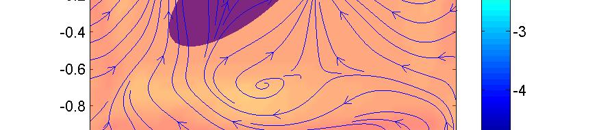
14 Figure 6: Streamlines of the flow for example 6.1 Third, using the extrapolated value of Q nn in the above step, Q n is linearly extrapolated to the whole domain along the normal vector field using: Q n τ + H 1 (n Q n Q nn ) = 0. (11) Finally, using the extrapolated value of Q n in the above step, Q is quadratically extrapolated to the whole domain along the normal vector field. Q τ + H 0 (n Q Q n ) = 0. (1) In [1], we introduced efficient discretizations for the above equations: We found that in order to obtain third order accuracy for the extrapolated quantity Q near the interface, it is enough to apply a TVD RK- discretization for the time derivative, a first order upwind discretization for the space derivatives in equations (10) and (11), and a second order ENO discretization for the space derivatives in (1). 6 Examples for the Navier-Stokes Equations 6.1 Convergence Analysis for an Exact Solution Consider the Navier-Stokes Equations on an irregular domain Ω = {(x, y) sin(x) sin(y). and 0 x, y π} with initial velocity field U(x, y, 0) = (sin x cos y, cos x sin y). The boundary condition of the velocity field on the wall is U bc n = 0. Figure 6 depicts the irregular domain and the streamlines of the flow. We take the appropriate forcing term for the exact solution to be U(x, y, t) = (cos t sin x cos y, cos t cos x sin y). We take a final time of π/3. Table 3 shows the second-order accuracy in the L 1 - and L - norms. 14

15 grid L norm order L 1 norm order 16.44E E E E E E E E E E Table 3: Convergence of the horizontal velocity in the case of the Navier-Stokes example on irregular domain for example Flow Past a Cylinder We now consider the simulation of a fluid flow past a cylinder, as first proposed by Dennis and Chang [5] and we show that our method is capable of reproducing the steady and unsteady regimes of the flows. The case where the Reynolds number is relatively small (Re 40) corresponds to a steady regime whereas larger Reynolds numbers (Re 00) correspond to unsteady regimes where vortex shedding can be observed. The transition between those two regimes occurs somewhere between Re = 40 and Re = 50, as demonstrated experimentally by Coutanceau and Bouard [4]. Consider a domain Ω = [0, 3] [016] and a cylinder with radius r =.5 and center located at (8, 8). We impose Dirichlet boundary conditions of u = U = 1 on the left, top and bottom walls, an outflux boundary condition at the right wall and the no-slip boundary condition at the cylinder s boundary. In our numerical experiments we define the viscosity coefficient µ = ru /Re and vary the Reynolds number Re. Figure 7 depicts the streamlines and vorticity contours for Re = 40. In particular, the symmetry of the results are in agreement with a steady regime for low Reynolds numbers. Figure 8depicts the streamlines and vorticity contours for Re = 50. This experiment illustrates a vertical asymmetry, indicating that the transition to an unstable regime occurs between Re = 40 and Re = 50. Figures 9 and 10 illustrates an unstable regime for Re = 100 and Re = 00, respectively. In particular, they exhibit the broken symmetry of the vorticity contours and the standard vortex shedding. The total force acting on the cylinder is is the integration of the force, and given as F = ( p + µd)n, Γ where D is the symmetric stress tensor and n is the outward normal to the cylinder. The drag and the lift coefficients are given by the x- and y- components of the F, respectively, properly scaled by ru. Figure 11 depicts the sinusoidal oscillations of the drag and lift coefficients on the cylinder. The coefficients, compared with earlier reports in table 6., are in agreement with those results. The integral for computing the force is approximated in this work by the geometric integration of [11]. 6.3 Flow Past Arbitrary Shaped Solid Objects Consider a domain Ω = [ 1, 1] with multiple solid obstacles as depicted in figure 1. We set a no-slip boundary on the solids boundaries, an inflow boundary condition of (u, v) = (1, 0) at x = 1 and an outflow boundary condition at x = 1. The top and bottom walls have a boundary 15

16 Figure 7: Stationary State : Contours of the stream functions and of the vorticity for Re = 40 of example 6.. The box in the figure is [7, 0] [6, 10]. Contour levels for the stream function are [ 5 : 0.05 : 5] and [ 0.05 : : 0.05]. Contour levels for the vorticity are [ 1 : 0.4 : 1]. Figure 8: Transition state : Contours of the stream functions and of the vorticity for Re = 50 of example 6. at t = 100. Contour levels and the dimensions of the box are the same as those in figure 7. The flow does not become stationary, and shows vertical asymmetry. 16

17 Figure 9: Unsteady Vortex Shedding state : Contours of the stream functions and of the vorticity for Re = 100 of example 6. at t = 100. The box in the figure is [7, 3] [5, 11]. Contour levels for the stream function are [ 5 : 0.1 : 5] and [ 0.05 : : 0.05]. Contour levels for the vorticity are [ 4 : 0. : 4]. Figure 10: Unsteady Vortex Shedding state : Contours of the stream functions and of the vorticity for Re = 00 of example 6. at t = 100. Contour levels and the dimensions of the box are the same as those in figure 9. 17

18 Figure 11: Time-dependent drag and lift coefficients for example 6.. (Top Left) Drag, Re=100; (Top right) Drag, Re=00); (Bottom left) Lift, Re=100; (Bottom right) Lift, Re=00. Drag(C D ) Lift(C L ) Re=100 Re=00 Re=100 Re=00 Belov et al. [] 1.19 ± 0.04 ±0.64 Braza et al. [] ± ± 0.05 ±0.5 ±0.75 Liu et al. [] ± ± ±0.339 ±0.69 Calhoun et al. [] ± ± ±0.98 ±0.668 Present ± ± ±0.360 ±0.74 Table 4: Drag and lift coefficients for example 6. 18

19 Figure 1: Streamlines contours for a flow past irregular shapes. 19

20 Figure 13:... condition of (u, v) = (1, 0). Figure 1 depicts the streamlines and the vorticity contours at steady state. as done in Ito et al. [?]. 6.4 Ellipse Falling in Flow with Interaction 7 Examples for the Navier-Stokes Equations in 3D 7.1 Convergence Analysis for an Exact Solution Consider the Navier-Stokes Equations on an irregular domain Ω = {(x, y, z) cos x cos y cos z.4 and.5π x, y, z 1.5π} with initial velocity field U(x, y, z, 0) = (cos x sin y sin z, sin x cos y sin z, sin x sin y cos z The boundary condition of the velocity field on the wall is U bc n = 0. We take the appropriate forcing term for the exact solution to be U(x, y, z, t) = (cos t cos x sin y sin z, cos t sin x cos y sin z, cos t sin x sin y cos z). We take a final time of π/3. Tables 5 and 6 show the first-order accuracy in the L - and L 1 - norms. Figures 15 through 16 show the log-log plot of the L - and L 1 - norms against grid resolution. 0

21 Figure 14:... 1

22 6 7 data best fit first order second order data best fit first order second order Figure 15: Log-log plots of the L (left) and L 1 (right) norms of the x and y components of velocity as a function of grid resolution for example data best fit first order second order data best fit first order second order Figure 16: Log-log plots of the L (left) and L 1 (right) norms of the z component of velocity as a function of grid resolution for example 7.1

23 grid L norm order L 1 norm order E- 4.9E E E E E E E E E Table 5: Convergence of the velocity in the x and y directions in the case of the Navier-Stokes example in 3D on irregular domain for example 7.1. grid L norm order L 1 norm order E- 7.55E E E E E E E E E Table 6: Convergence of the velocity in the z direction in the case of the Navier-Stokes example in 3D on irregular domain for example Flow Past a Sphere We now consider the simulation of a fluid flow past a sphere, as presented by Johnson and Patel [?] and show that our method is capable of reproducing the steady axissymmetric flow and steady non-axissymmetric flow regimes (results for unsteady vortex shedding regime pending). Steady axissymmetric flow occurs at relatively low Reynolds number (Re 150) while the steady nonaxissymmetric flow occurs at larger Reynolds numbers (Re 50). The transition between those two regimes occurs somewhere between Re = 00 and Re = 10. Consider a domain Ω = [0, 16] [0, 8] [0, 8] and a sphere with radius r =.5 and center located at (4, 4, 4). We impose Dirichlet boundary conditions of u = U = 1 on the left, top, bottom, front, and back walls, an outflux boundary condition at the right wall and the no-slip boundary condition at the sphere s boundary. In our numerical experiments we define the viscosity coefficient µ = ru /Re and vary the Reynolds number Re. Figure 17 depicts the particle path trace for a steady axissymmetric flow in 3D at Re = 150. Figures 18 and 19 depict the streamlines and vorticity contours at Re = 150. In particular, the symmetry of the results are in agreement with a steady axissymmetric flow regime for lower Reynolds numbers, and are comparable to the results obtained by [?](Figures 3 and 7). Figures 0 through depict the streamlines contours, vorticity contours, and three-dimensional particle path trace for Re = 50 corresponding to the steady nonaxissymmetric flow regime for larger Reynolds number. The results are in good agreement with results obtained by [?] (Figures 11, 1, and 14). (TODO:Graphs, short explanation on the tilted plane of symmetry, Re50 projected vorticities) 3

24 Figure 17: Steady Axissymmetric Regime: Particle path trace in 3D for the Re = 150 case of example 7.. 4

25 Figure 18: Steady Axissymmetric Regime: Streamlines projected on the x-y plane for the Re = 150 case of example 7.. Top: our results, bottom: results from [?]. 5

26 Figure 19: Steady Axissymmetric Regime: Vorticity contours for the curl of velocity around the z-axiz for the Re = 150 case of example 7.. Contour levels are [ 5 :.5 : 5]. Top: our results, bottom: results from [?] 6

27 Figure 0: Steady Non-Axissymmetric Regime: Streamlines projected on the x-y plane(top) and x-z plane(bottom) for the Re = 50 case of example 7.. Left column: our results, right column: results from [?]. 7

28 Figure 1: Steady Non-Axissymmetric Regime: Vorticity contours for the curl of velocity around the z-axiz for the Re = 50 case of example 7.. Contour levels are [ 5 :.5 : 5]. Top: our results, bottom: results from [?]. 8

29 Figure : Steady Non-Axissymmetric Regime: Particle path trace from the x-y view(top), x-z view(middle), and y-z view(bottom) for the Re = 50 case of example 7.. Left column: our results, right column: results from [?]. 9

30 Figure 3: Curl of velocity and streamlines around the x-axis, viewed down the positive x-axis (left) and negative x-axis (right). 7.3 Ellipse Translated and Rotated in Flow Consider a domain Ω = [ 1, 1] [ 1, 1] [ 1, 1] and an ellipsoid with dimensions radius x =.5, radius y = radius z =., centered at (., 0, 0) at tn = 0, and rotating around the pivot point (0, 0, 0). We impose no-slip boundary conditions all the domain walls and the ellipsoid boundary. We define viscosity µ =.0001 and angular velocity ω =.5 in the clockwise direction around the z-axis. Figures 3 through 5 depict the streamline slices and curl of velocity around the x, y, and z axes. In figure 5, the streamlines and curl of velocity is symmetric on both sides of the z = 0 plane, since the rotation of the ellipsoid is around the z-axis only. 8 Conclusion We have presented a novel and efficient projection method for the Navier-Stokes equations on irregular domains. The irregular domains can be of arbitrary shape and do not have to be approximated by domain s rasterization. This method is straightforward to implement and leads to a symmetric positive definite linear system that can be inverted efficiently with standard iterative methods. We demonstrated the second-order accuracy in the L 1 and L norms and showed that this method can reproduce accurate fluid flow motions on irregular domains. 9 Acknowledgments The research of C. Min was supported in part by the Kyung Hee University Research Fund (KHU ) in 007 and by the Korea Research Foundation Grant funded by the Korean Government (MOEHRD, Basic Research Promotion Fund) (KRF C00045). The research of F. Gibou was supported in part by a Sloan Research Fellowship in Mathematics, by the National Science Foundation under grant agreement DMS and by the Department of Energy under grant agreement DE-FG0-08ER

31 Figure 4: Curl of velocity and streamlines around the y-axis, viewed down the positive y-axis (left) and negative y-axis (right). References [1] T. Aslam. A partial differential equation approach to multidimensional extrapolation. J. Comput. Phys., 193: , 004. [] C. Batty, F. Bertails, and R. Bridson. A fast variational framework for accurate solid-fluid coupling. ACM Trans. Graph. (SIGGRAPH Proc.), 6(3), 007. [3] A. Chorin. A Numerical Method for Solving Incompressible Viscous Flow Problems. J. Comput. Phys., :1 6, [4] M. Coutanceau and R. Bouard. Experimental determination of the main features of the viscous flow in the wake of a circular cylinder in uniform translation. part 1. steady flow. J. Fluid. Mech., 79:31, [5] S. Dennis and G. Chang. Numerical solutions for seady flow past a circular cylinder at Reynolds number up to 100. J. Fluid. Mech., 4:471, [6] F. Gibou and R. Fedkiw. A fourth order accurate discretization for the Laplace and heat equations on arbitrary domains, with applications to the Stefan problem. J. Comput. Phys., 0: , 005. [7] F. Gibou, R. Fedkiw, L.-T. Cheng, and M. Kang. A second order accurate symmetric discretization of the Poisson equation on irregular domains. J. Comput. Phys., 176:05 7, 00. [8] C. Hirt, A. Amsden, and J. Cook. An arbitrary Lagrangian-Eulerian computing method for all flow speeds. J. Comput. Phys., 135:7 53,

32 Figure 5: Curl of velocity and streamlines around the z-axis, at slice z = 0(top left), z = ±.1 (top right), z = ±.(bottom left), and z = ±.3(bottom right). 3

33 [9] R. LeVeque and Z. Li. The immersed interface method for elliptic equations with discontinuous coefficients and singular sources 31: , SIAM J. Numer. Anal., 31: , [10] C. Min and F. Gibou. A second order accurate projection method for the incompressible Navier-Stokes equation on non-graded adaptive grids. J. Comput. Phys., 19:91 99, 006. [11] C. Min and F. Gibou. Geometric integration over irregular domains with application to level set methods. J. Comput. Phys., 6: , 007. [1] C. Min and F. Gibou. A second order accurate level set method on non-graded adaptive Cartesian grids. J. Comput. Phys., 5:300 31, 007. [13] S. Osher and R. Fedkiw. Level Set Methods and Dynamic Implicit Surfaces. Springer-Verlag, 00. New York, NY. [14] C. Peskin. Flow patterns around heart valves: A numerical method. J. Comput. Phys., 10:5 71, 197. [15] J. A. Sethian. Level set methods and fast marching methods. Cambridge University Press, Cambridge. [16] D. Xiu and G. Karniadakis. A semi-lagrangian high-order method for Navier-Stokes equations. J. Comput. Phys, 17: ,