Finite Difference Method

Transcription

1 Finite Difference Method for BVP ODEs Dec 3,

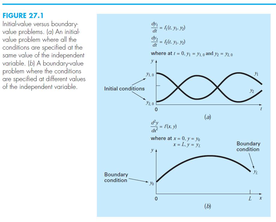
2 Recall An ordinary differential equation is accompanied by auxiliary conditions. In the analytical method, these conditions are used to evaluate the constants of integration that result during the solution of the equation. For an nth-order equation, n conditions are required. If all the conditions are specified at the same value of the independent variable, then we are dealing with an initial-value problem. In contrast, there is another application for which the conditions are not known at a single point, but rather, are known at different values of the independent variable. Because these values are often specified at the extreme points or boundaries of a system, they are customarily referred to as boundary-value problems. 2

3 3

4 Shooting Method, Example Problem 4

5 Example.. The conservation of heat can be used to develop a heat balance for a long, thin rod (previous slide). If the rod is not insulated along its length and the system is at a steady state, the Temperature T along the rod can be given by the above equation. where h is a heat transfer coefficient (m 2 ) that parameterizes the rate of heat dissipation to the surrounding air and Ta is the temperature of the surrounding air. For L= 10-m rod T a = 20, T 1 = 40, T 2 = 200 h = Using the analytical method 5

6 Example The second-order equation can be expressed by a change of variables as two first order ODEs: 6

7 Example Let s deal with the BCs: The second-order equation can be expressed as two first order ODEs: To solve these equations, we require an initial value for z. We don t have it For the shooting method, we guess a value, e.g. z(0) = 10. 7

8 Example Using a fourth-order RK method with a step size of 2, we obtain a value at the end of the interval of T(10) = ,which differs from the boundary condition of T(10) = 200. Therefore, we make another guess, z(0) = 20, and perform the computation again. This time, the result of T(10) = is obtained. GUESS Computed Value Quality? z(0)=10 T(10)= LOW INTERPOLATE T(10)= 200 REAL z(0)=20 T(10)= HIGH 8

9 Example Now interpolate!! GUESS Computed Value Quality? z(0)=10 T(10)= LOW INTERPOLATE T(10)= 200 REAL z(0)=20 T(10)= HIGH Linear interpolation gives you a new guess 9

10 Example The second-order equation can be expressed as two first order ODEs: After linear interpolation, the guess becomes. z(0) =

11 The cartoon view 11

12 Finite Difference Method The main feature of the finite-difference method is to obtain discrete equations by replacing derivatives with appropriate finite divided differences. We derive and solve a finite difference system for the BVP in four steps. 1. Discretization of the domain of the problem 2. Discretization of the differential equation at the interior nodes 3. The third step is devoted to the treatment of the boundary conditions. 4. Solve the system of linear equations. The linear system is tridiagonal, and the solution of tridiagonal linear systems is a very well-studied problem. 12

13 13

14 A y b 14

15 Finite Difference Method for BVP The previous matrix equations can be solved easily using MATLAB For instance: % Finite Difference Method clc, clear A=[ some matrix of coefficients]; b=[some RHS vector]; y=a\b % y is the vector solution % That s it!!!!!!!!!!!!!!!!!!!!!!!!!!!!!!!!! % but you should graph the solution? 15