NEW FAMILIES OF EMBEDDED TRIPLY PERIODIC MINIMAL SURFACES OF GENUS THREE IN EUCLIDEAN SPACE. Adam G. Weyhaupt

Transcription

1 NEW FAMILIES OF EMBEDDED TRIPLY PERIODIC MINIMAL SURFACES OF GENUS THREE IN EUCLIDEAN SPACE Adam G. Weyhaupt Submitted to the faculty of the University Graduate School in partial fulfillment of the requirements for the degree Doctor of Philosophy in the Department of Mathematics Indiana University 4 August 2006

2 Accepted by the Graduate Faculty, Indiana University, in partial fulfillment of the requirements for the degree of Doctor of Philosophy. Matthias Weber, Ph.D. Jiri Dadok, Ph.D. Bruce Solomon, Ph.D. Peter Sternberg, Ph.D. 4 August 2006 ii

3 Copyright 2006 Adam G. Weyhaupt ALL RIGHTS RESERVED iii

4 To Julia my source of strength, my constant companion, my love forever and to Brandon and Ryan whose exuberance and smiles lift my spirits daily and have changed my life in so many wonderful ways. iv

5 Acknowledgements I can not imagine having completed graduate school with a different advisor: thank you, Matthias Weber, for your encouragement, your guidance, your constant availability, and for making me feel like a colleague. The following exchange is typical of my interaction with him: Me:... I need an infusion of optimism and a fresh pair of eyes. Him: It s ok. Can t promise fresh ice, but as infusion there will be tea. Especially, thank you for introducing me to the beautiful study of minimal surfaces. Thank you to the other members of my committee for their improvement of this work; I have particularly been helped by conversations throughout the years with Jiri Dadok. My time at Indiana has been enjoyable and fruitful because of innumerable people, most of whom I will undoubtedly forget to mention. Particularly, I thank Misty Cummings for ensuring that I (and all the graduate students) haven t run administratively amuck; Kent Orr for enjoyable discussions about math and family; and Jennifer Franko, Noah Salvaterra, and Eric Wilson for being my colleagues and friends through these changing years (and without whose companionship while studying I might not have passed my Tier 1 exams). Prior to Indiana, my teachers at Marquette Catholic High School and Eastern Illinois University helped to form me into an academic, especially Peter Andrews, Charles Delman, Greg Galperin, Lou Hencken, Suzer Phelps, Ira Rosenholz, Rosemary Schmalz, Margaret Weaver, and Keith Wolcott. Thinking back about you all reminds me that, as a teacher, nearly everything we do can impact our students. Education has always been a focus in my life, thanks to my mother and father who have always encouraged me to study hard, get a good job, and do something I enjoy. They have given me many opportunities and much encouragement through these years, and I am forever grateful. The memory of my grandfather, Joseph Weyhaupt, encourages me to work v

6 harder and supports me when I m feeling low, and the rest of my family is always there for me. My own family, Julia, Brandon, and Ryan, have put up with so much through these years and have always encouraged me and stood with me. You have never been a hindrance, but rather, have given me three wonderful reasons to continue. I am grateful to the National Science Foundation, who has funded much of my graduate existence these five years through a VIGRE fellowship, and to the American Institute of Mathematics for support at the AIM workshop Moduli Spaces of Properly Embedded Minimal Surfaces (thanks also to the organizers for the invitation). I feel connected to the minimal surface community as a result of this workshop. Further financial support for travel from Indiana University, Rice University, Northwestern University, and the University of Michigan is appreciated. vi

7 Abstract Until 1970, all known examples of embedded triply periodic minimal surfaces (ETPMS) contained either straight lines or curves of planar symmetry. In 1970, Alan Schoen discovered the gyroid, an ETPMS that contains neither straight lines nor planar symmetry curves. Meeks discovered in 1975 a 5-parameter family of genus 3 ETPMS that contained all known examples of genus 3 ETPMS except the gyroid. A second example lying outside the Meeks family was proposed by Lidin in Große-Brauckmann and Wohlgemuth showed in 1996 the existence and embeddedness of the gyroid and Lidinoid. In a series of investigations the scientists, Lidin, et. al., numerically indicate the existence of two 1-parameter families of ETPMS that contain the gyroid and one family that contains the Lidinoid. In this thesis, we prove the existence of these families. To prove the existence of these families, we describe the Riemann surface structure using branched covers of non-rectangular tori. The 1 holomorphic 1-forms Gdh, Gdh, and dh each place a cone metric on the torus; we develop the torus with this metric into the plane and describe the periods in terms of these flat structures. Using this description of the periods, we define moduli spaces for the horizontal and vertical period problems so that Weierstraß data (X, G, dh) solves the period problem if the flat structures of X induced by these 1-forms are in the moduli spaces. To show that there is a curve of suitable data, we use an intermediate value type argument. vii

8 Contents Chapter 1. Introduction Applications of the flat structure technique to the classification of triply periodic minimal surfaces Survey of techniques used Outline of dissertation 9 Chapter 2. Preliminaries Weierstraß data and the period problem Theta functions Some facts about triply periodic minimal surfaces Cone metrics and Schwarz-Christoffel maps on tori 21 Chapter 3. Symmetries and Quotients (Outline of a Classification) Classification by symmetries Classification by conformal automorphisms 40 Chapter 4. Review of Known Examples The P Surface and tp deformation The gyroid The H surface The Lidinoid The P Surface from the standpoint of an order 3 symmetry The CLP surface 78 Chapter 5. Proof of the Existence of the Gyroid and Lidinoid Families Horizontal and vertical moduli spaces for the tg family 85 viii

9 5.2. Proof of the tg family Moduli spaces for the rl family of Lidinoids Moduli spaces for the rg family of gyroids 102 Chapter 6. Questions, Conjectures, and Future Work 106 Appendix A. Calculation of ρ and τ for the Schwarz P surface 113 A.1. Calculation of ρ 113 A.2. Calculation of τ 115 Bibliography 117 ix

10 CHAPTER 1 Introduction As early as 1762, Lagrange s newly developed calculus of variations broached the problem of finding the surface of smallest area with a prescribed space curve as its boundary. (The general problem of determining the existence and properties of minimizing surfaces with prescribed space curve boundary is called the Plateau problem.) He derived the partial differential equation which must be satisfied by all such surfaces. Explicit examples of such surfaces were provided by Euler (the catenoid, shortly before 1762) and Meunsier (the helicoid, around 1765) [Nit75]. All such area minimizing surfaces have vanishing mean curvature H. In modern language, the study of minimal surfaces is the study of all real 2-dimensional surfaces in R 3 with H 0. Locally, these surfaces minimize area with respect to the boundary (of the local surface patch). All complete minimal surfaces without boundary are necessarily non-compact. In this thesis, we are concerned with the study of triply periodic minimal surfaces. A triply periodic minimal surface is a minimal surface M that is invariant under the action of a rank 3 lattice Λ. M is, of course, non-compact; we often work with the much more tractable quotient M/Λ which is compact. The ultimate goal of the study of triply periodic minimal surfaces is to classify all embedded triply periodic minimal surface of a fixed genus. Many examples are known. The first examples of a triply periodic minimal surface were given by Schwarz [Sch90] in 1865 when he exhibited the P, D, and H surfaces (see Figure 1.2). Early examples were constructed by solving the Plateau problem for non-planar polygons in space, such as on some of the edges of a cube (see Figure 1.1). After considerable attention in the late nineteenth and early twentieth centuries, triply periodic minimal surfaces experienced a slow-down of activity until the late 1960 s, when physical scientists began to investigate them for possible 1

11 1. INTRODUCTION 2 applications to materials science, biology, and chemistry. Chemists and materials scientists are now finding triply periodic minimal surfaces in images (on the nanometer scale) of the interface between two compounds in block co-polymers. They believe that the geometry of these interfacial surfaces significantly influence the physical properties of the compound [TAHH88, FH99]. Biologists have identified triply periodic minimal surfaces as membranes in certain cellular structures [DM98]. Figure 1.1. The D surface solves the Plateau problem for the highlighted contour. Figure 1.2. (left) A translational fundamental domain of the Schwarz P surface. (right) A fundamental domain of the Schwarz H surface.

12 1. INTRODUCTION 3 In 1970, Alan Schoen [Sch70], a NASA crystallographer interested in strong but light materials, showed the existence of 12 previously undiscovered triply periodic minimal surfaces. Among these was the gyroid, an embedded surface containing no straight lines or planar symmetry curves (unlike other known examples at the time) [Kar89, GBW96]. In his 1975 Ph.D. thesis, Bill Meeks [Mee75] discovered a 5-parameter family of embedded genus 3 triply periodic minimal surfaces. Specifically, Theorem 1.1 (Meeks, 1975). There is a real five-dimensional family V of periodic hyperelliptic Riemann surfaces of genus three. These are the surfaces which can be represented as two-sheeted covers of S 2 branched over four pairs of antipodal points. There exists two distinct isometric minimal embeddings for each M 3 V. The Meeks family contained all triply periodic minimal surfaces of genus 3 known at that time except for the gyroid. (In fact, most of the members of the Meeks family were previously undiscovered surfaces. Many surfaces in his family have no straight lines and no planar symmetries.) In 1990, Sven Lidin discovered a related surface, christened by Lidin the HG surface but commonly called the Lidinoid [LL90]. (Minimal surface nomenclature leaves much to be desired. One of Schoen s surfaces is typically called Schoen s Unnamed Surface Number 12. We do not help this any by adopting in this work the notation of Fogden, Haeberlein, and Lidin in [FHL93].) Although Schoen s surfaces were studied by crystallographers and physical scientists early on, it was not until the early 1990 s that these surfaces entered the mathematical mainstream. In 1995, Große-Brauckmann and Wohlgemuth [GBW96] proved that the gyroid and Lidinoid are embedded. The Meeks family ensures that every currently known triply periodic minimal surface except for the gyroid and Lidinoid is deformable, i.e., for each triply periodic minimal surface M (M not the gyroid or Lidinoid) there is a continuous family of embedded triply periodic minimal surfaces M η, η ( ɛ, ɛ) such that M = M 0. Note that, in general, the lattices may vary with η, so that generically Λ η1 Λ η2 (we conjecture that it is never the case that the lattice is constant in a deformation, see Conjecture 6.1). We are primarily concerned with the following question:

13 1. INTRODUCTION 4 main question. Do there exist continuous deformations of the gyroid and the Lidinoid? In a series of papers, the crystallographers and physical chemists Fogden, Haeberlein, Hyde, Lidin, and Larsson numerically indicate the existence of two 1-parameter families of embedded triply periodic minimal surfaces that contain the gyroid and two additional families that contain the Lidinoid [FHL93, FH99, LL90]. While even accompanied by very convincing computer-generated images, their work does not provide an existence proof, and the mathematical landscape is fraught with examples where pictures mislead (see, for example, [Web98]). Our main result of this thesis, then, is: Theorem 1.2. There is a one parameter family of minimal embeddings tg η R 3 /Λ η, η R +, such that tg η is an embedded minimal surface of genus 3.The gyroid is a member of this family. Furthermore, each tg η admits a rotational symmetry of order 2. (Note that the t is not a parameter. The t stands for tetragonal ; [FHL93] call this a tetragonal deformation because crystallographers typically call a deformation of a cubical lattice tetragonal if the lattice admits an order 2 rotational symmetry throughout the deformation.) This shows that the gyroid is deformable. Our other two main theorems prove the existence of a Lidinoid family and an additional gyroid family: Theorem 1.3. There is a one parameter family of minimal embeddings rl η R 3 /Λ η, η R +, such that rl η is an embedded minimal surface of genus 3.The Lidinoid is a member of this family. Furthermore, each rl η admits a rotational symmetry of order 3. Theorem 1.4. There is a one parameter family of minimal embeddings rg η R 3 /Λ η, η R +, such that rg η is an embedded minimal surface of genus 3.The gyroid is a member of this family. Furthermore, each rg η admits a rotational symmetry of order 3. Since the Lidinoid also admits an order 2 symmetry similar to the gyroid, we would expect to obtain a family of Lidinoids that preserves an order 2 symmetry. A survey of the literature seems to turn up no such family; a preliminary analysis shows that this family would be distinctly different conformally, and we defer its investigation to a future paper. As a consequence of these results, we have shown:

14 1. INTRODUCTION 5 All currently known examples of genus 3 triply periodic minimal surfaces admit deformations. As far as we know, none of these new examples are members of the Meeks family Applications of the flat structure technique to the classification of triply periodic minimal surfaces Perhaps the most ambitious problem in the theory of triply periodic minimal surfaces is to obtain a classification. In addition to constructing families of gyroids and Lidinoids, we also outline a method for approaching a classification of triply periodic minimal surfaces using techniques similar to those in the construction of the families. While we do not obtain any new families with this approach, we are able to classify surfaces that have sufficiently many symmetries. Since the surface M/Λ is compact in the flat 3-torus R 3 /Λ, it is most natural to first consider a classification by genus. Theorem 1.5 (Meeks, 1975). If M/Λ R 3 /Λ is a connected triply periodic minimal surface of genus g, then g 3. In early 2006, Martin Traizet [Tra06] showed that Theorem 1.6. For any flat 3-torus R 3 /Λ and for any integer g 3, there exists a sequence of orientable, compact, embedded minimal surfaces M n R 3 /Λ which have genus g. Moreover, the area of M n goes to infinity as n. (In the case of genus 3 surfaces, Traizet explicitly computes only one example; this is a known example in the Meeks family. However, Traizet mentions that we find numerically that there are other balanced configurations which are not as symmetric as the one we discussed... [t]his confirms the already suspected fact that the space of genus 3 minimal surfaces in a 3-torus is quite intricate. It is quite possible that these additional surfaces are previously undiscovered. Nonetheless, Traizet s construction method ensures that these surface come in a family, so our statement about all currently known surfaces admitting deformations remains true.)

15 1. INTRODUCTION 6 In this thesis, we concentrate on the topologically most simple case; all surfaces M we consider have genus 3. There are two types of classification questions we consider. The first can be loosely described as follows: given a fixed set of symmetries, what genus 3 embedded triply periodic minimal surfaces admit these symmetries? The flat structure approach is well-suited to this type of investigation, because the presence of symmetries allows one to narrow the moduli spaces to consider, creating problems that, in principle, are easier to solve. In Chapter 3, we obtain a classification for certain fixed symmetries. The motivation here is the P surface, which provides a model surface with a large number of symmetries. For example, one of the results we obtain in Chapter 3 is theorem Let M be an embedded triply periodic minimal surface of genus 3 that admits a rotational symmetry ρ of order 3 about an axis L in R 3. Assume that M/Λ admits a reflection in a plane containing L so that the fixed point set in M/Λ/ρ consists of two components. Then M is a member of the rp D or rh families. On the other hand, any complete classification would have to consider surfaces with essentially no symmetries. Here, the gyroid and Lidinoid families that we have constructed could be useful examples in the study of such surfaces. In particular, Traizet s method of opening nodes around a set of balanced points [Tra02, Tra06] may be a useful approach. A full understanding of the families indicated here may provide examples of new balanced configuration that can be exploited using Traizet s technique. At the very least, one could hope for a larger family of gyroids than a 1-parameter family Survey of techniques used Here we briefly indicate some of the techniques employed by others to construct triply periodic minimal surfaces. Each is useful in certain contexts, but are a modification of several methods is necessary for constructing gyroid families Survey of techniques used by other authors. One method for constructing triply periodic surfaces is the conjugate Plateau method, a general tool useful in many settings (even in non-euclidean space forms). It was employed by Karcher [Kar89, Kar05]

16 1. INTRODUCTION 7 to construct many surfaces and their deformations; surfaces that have fundamental domains bounded by straight lines or planar symmetry curves are well-suited for this method. Karcher s method transforms the problem into one of finding a minimal disk with boundary a polygon in R 3. Since the gyroid contains neither straight lines nor planar symmetry curves [Kar89], we cannot make use of this construction. Meeks obtains his 5-parameter family by exploiting a hidden symmetry that many surfaces share. Every genus 3 surface can be represented conformally as a two-sheeted branched cover of S 2 with eight branch points (Proposition 2.10). Meeks considers only those surfaces which are branched over four pairs of antipodal points on the sphere. In homogeneous coordinates on CP 1 = S 2, the antipodal map is represented by z 1 z. He then obtains a map f from the 2-fold branch cover of the sphere to C 3 /L, where L is a (complex) lattice in C 3. That this construction is invariant under complex conjugation implies the existence of two rank 3 invariant sublattices, namely, representing the real and imaginary sublattices. Then the maps Re f and Im f provide the two distinct embeddings of the branched sphere. The period problem is automatically solved because of the invariance of this sublattice. The 5-parameter family comes from 8 parameters possible from picking four of the branch points, less 3 parameters since scaling and rotation is not considered a deformation in any reasonable sense. Meek s method fails to produce gyroid or Lidinoid examples, however, since neither is in a real or imaginary subspace of their embedding, as we shall see in the construction of the gyroid in Section 4.2. A third method involves the modification of certain holomorphic data that describe a minimal surface. Minimal surfaces are described by three data (called the Weierstraß data): a meromorphic function G and a holomorphic 1-form dh defined on a Riemann surface X. G, the Gauß map or stereographic projection of the normal map, is a meromorphic function on a minimal surface. After choosing a base point p X, the 1-forms ω 1 = 1 2 ( 1 G G)dh, ω 2 = i 2 ( 1 G + G)dh, and w 3 = dh parameterize the minimal surface as the image of F : X R 3 defined by z z z ) (1.1) F (z) = Re( ω 1, ω 2, ω 3

17 1. INTRODUCTION 8 Furthermore, given a Riemann surface, any meromorphic G and holomorphic 1-form dh that satisfy ω ω2 2 + ω2 3 0 (and ω ω ω 3 2 0) yield a minimal surface (in general, this surface is not even immersed). One method of constructing surfaces is to find compatible G and dh (along with a Riemann surface) that give an immersed minimal surface. Immersion is accomplished by solving the period problem: closed curves on the Riemann surface must map under Equation 1.1 to closed curves in space (or, in the case of triply periodic minimal surfaces, closed curves in the 3-torus). (We make these notions precise in Section 2.1.) Except in the most simple cases, however, (and certainly for the gyroid) this period problem is difficult to solve: the required dh alone is determined by an unwieldy elliptic integral. Constructing a family in this way would require the simultaneous control of three elliptic integrals, a task best suited for numerical computation. Finally, a new technique employed by Traizet shows great promise in constructing minimal surfaces. For technical details, we refer the reader to [Tra02, Tra06]. Compare Figures 4.5, 4.14, and In each case, as τ 0, the surfaces limit to a lamination of R 3 by planes with tiny (singular) catenoidal necks placed periodically throughout. Traizet derives a set of balancing equations that, if satisfied by a set of points on k-distinct planes (the balancing equations have interaction between adjacent planes) can construct a minimal surface family. To construct the family, Traizet opens nodes at the singularities to obtain a Riemann surface. These tiny catenoidal necks are opened using a modification of the implicit function theorem. The period problem is solved because of the balancing equations. The difficulty, then, is finding solutions to the balancing equations that yield interesting surfaces. We find it quite appealing that these balanced points can be considered as electrostatic forces in a stable configuration. Since we have no suggestions of what a limit of gyroids might look like, we have no guidance for finding an appropriate set of points that might yield a gyroid family. We hope that Traizet s method could be employed to study the gyroid after we more fully understand the families we have constructed here Overview of proof. We instead construct our family using the flat structure method introduced in [WW98]. To construct a family of surfaces M t, we first start with

18 1. INTRODUCTION 9 an embedded surface M 0. This surface will have many symmetries, and we fix a symmetry that we want the entire family to have; for instance, all M t will be invariant under rotation by π about a vertical axis. This gives as an appropriate conformal model for our family of surfaces a two fold (since the rotation has order 2) branched cover of a torus. In order for the surfaces to be immersed, we need to solve the period problem, that is, we need closed cycles on the branched cover of a torus to map to closed cycles on M t /Λ t R 3 /Λ t for 1 some lattice Λ t. We introduce the holomorphic 1-forms Gdh, Gdh, and dh; these induce cone metrics on the torus which allow us to understand the periods of these forms in terms of Euclidean polygons (these polygons are the development of the cone metric induced on the torus by the 1-form into the Euclidean plane). We describe two moduli spaces of polygons one for the horizontal period problem and one for the vertical period problem; these spaces have the property that when the developed flat structures are contained in the moduli spaces, the period problem is solved. The problem of finding a family of surfaces is therefore reduced to showing that there exists a curve of Weierstraß data (a torus which gives a conformal model, and a Gauß map and height differential) so that the developed flat structures are in these moduli spaces. We obtain this curve nonconstructively as the zero set of a certain map. Embeddedness is a consequence of the continuity of the construction and the maximum principle for minimal surfaces Outline of dissertation We begin in Chapter 2 with a discussion of the major tools used to construct the new families of surfaces: the Weierstraß data, theta functions, and cone structures on tori. We also include a selection of facts about triply periodic minimal surface that provide a window into the current status of a classification. In Chapter 3, we provide a framework for classifying triply periodic minimal surface of genus 3 using the flat structure technique. After assuming the presence of sufficiently many symmetries, we are able to classify all embedded, genus 3 triply periodic minimal surfaces admitting these symmetries.

19 1. INTRODUCTION 10 In Chapter 4, we begin the heart of the thesis by reviewing several known examples of triply periodic minimal surfaces. In each case considered here, we obtain a continuous family of minimal surfaces. This chapter also will construct the gyroid and Lidinoid using the perspective in Chapter 3 and the tools in Chapter 2. (We relegate some technical details from the construction of the P surface to Appendix A.) Again, we explore each surface using flat structures. In Chapter 5, we set up the moduli spaces used to solve the period problem for each of the two gyroid families tg and rg and for the Lidinoid family rl. We prove in Chapter 5 the existence of the tg family in detail. The existence of the other two families are proved similarly, and we indicate any significant differences when describing the moduli spaces. Finally, Chapter 6 contains a collection of questions and conjectures for future investigation. In particular, we indicate a number of questions that could be used to expand the classification framework to a more general classification. Also, we indicate here a number of questions about the gyroid and Lidinoid families.

20 CHAPTER 2 Preliminaries Minimal surfaces have been profitably studied both from a geometric viewpoint and from the perspective of partial differential equations. We take the geometric viewpoint, where the foundational tool is the ability to describe minimal surfaces using the Weierstraß data Weierstraß data and the period problem For this section, we refer the reader to [DHKW92, Oss69, Nit75] for further details and history. Let Ω C denote a simply connected open domain and let h = (h 1, h 2, h 3 ) : Ω C 3 be a non-constant holomorphic map so that h h2 2 + h2 3 0 and h 1(z) 2 + h 2 (z) 2 + h 3 (z) 2 0 z Ω. A direct computation shows that F : Ω R 3 defined by (2.1) p Re p (h 1 dz, h 2 dz, h 3 dz) is a minimal surface M R 3. The normal map, N : M S 2 assigns to each point p M the normal at p. The Gauß map, G : M C is the stereographic projection of the normal map. (Of course, all of this discussion of the normal map and stereographic projection depends upon the choice of orientation and of projection. The results are, of course, independent of choice.) 2.1 as To relate Equation 2.1 to the geometry of the surface, note that we can rewrite Equation (2.2) p Re p ( G G, i ) G + ig, 1 dh. The meromorphic function G in Equation 2.2 is the Gauß map: (2.3) G = h 1 + ih 2 h 3. 11

21 2. PRELIMINARIES 12 (dh is a holomorphic differential, often called the height differential.) Furthermore, given any minimal surface M, there exists a height differential dh so that it, along with the Gauß map, provide the above parameterization of a surface patch. Therefore, simply connected surface patches are fully parameterized. The following result of Osserman gives us a way to parameterize non-simply connected surfaces. Theorem 2.1 (Osserman, [Oss69]). A complete regular minimal surface M having finite total curvature, i.e. M K da <, is conformally equivalent to a compact Riemann surface X that has finitely many punctures. Notice that since our triply periodic minimal surfaces M are compact in the quotient M/Λ, they necessarily have finite total curvature and therefore can be parameterized on a Riemann surface. Instead of using a simply connected domain Ω and meromorphic functions h 1, h 2, h 3, we instead consider three holomorphic 1-forms ω 1, ω 2, ω 3 defined on a Riemann surface X, again with ωi 2 0 and ω i 2 0 (making sense of this first quantity pointwise and locally). We can then write (2.4) F : X R 3 by p Re with p (ω 1, ω 2, ω 3 ) (2.5) ω 1 = 1 2 ( 1 G G)dh ω 2 = i 2 ( 1 G + G)dh w 3 = dh. Since the domain is no longer simply-connected, integration of the Weierstraß data over a homotopically non-trivial loop γ on X is generically no longer zero. This integration leads to a translational symmetry of the surface. 1 We define the period of γ by (2.6) P (γ) := Re (ω 1, ω 2, ω 3 ). γ 1 The surface need not, at this point, be embedded or even immersed, so the term symmetry is perhaps misleading here. More precisely, if F (p) = (q 1, q 2, q 3) R 3 for some choice of path of integration from the base point to p, then for any other choice of path of integration, F (p) = (q 1, q 2, q 3) + R (ω1, ω2, ω3) for some γ γ H 1(X, Z).

22 2. PRELIMINARIES 13 In order for a surface to be non-periodic, we must have P (γ) = 0 for all γ H 1 (X, Z). For a surface to be triply periodic with lattice Λ R 3, we must have (2.7) P (γ) Λ γ H 1 (X, Z). Notice that we can write (2.8) F 1 (z) + if 2 (z) = z so we can instead write the periods as ( Re γ Gdh + γ ( (2.9) P (γ) = Im γ Gdh + γ Re γ dh z 1 Gdh + G dh, ) 1 G dh ) 1 G dh. Lemma 2.2. Let X be a Riemann surface of genus g. Let G : X C be meromorphic, and let dh be a holomorphic 1-form defined on X. Furthermore, assume that (1) if G has a zero or pole of order k at p, then dh also has a zero at p. Conversely, if dh has a zero of order k at p, then G must have a zero or pole of order k at p. (2) there exists a lattice Λ R 3 such that for all γ H 1 (X, Z), P (γ) Λ. Then the Weierstraß data (X, G, dh) define an immersed triply periodic minimal surface of genus g. Proof. Define ω i as described in Equation 2.5. One trivially checks that i ω2 i 0. We need only to see that i ω i 2 never vanishes. Since (2.10) ω i 2 = 1 ( G + 1 ) dh, 2 G i Condition 1 is precisely what is needed so that the right hand side of Equation 2.10 is non vanishing. Incidentally, the quantity in Equation 2.10 is the square of the conformal stretch factor ds (hence the reason why it must not vanish). The problem of finding data so that Condition 2 is satisfied is often called the period problem (or, more violently, killing periods).

23 2. PRELIMINARIES 14 The Weierstraß representation immediately indicates the following well-known construction of a minimal surface. Let M 0 be a minimal surface defined by Weierstraß data (X, G, dh). 2 We construct a new minimal surface M θ using Weierstraß data (X, G, e iθ dh). Note that the data still satisfies the requirements of Lemma 2.2, especially that j e2iθ ωj 2 0. The family of surfaces M θ (0 θ π 2 ) is called the associate family of M 0. (Sometimes these surfaces M θ are also called the Bonnet transformation of M 0.[Nit75, Bon53] ) Notice that if the period problem is solved for M 0, it will in general not be solved for M θ, since P Mθ (γ) is a linear combination of P M0 (γ) and P M π2 (γ), which need not be either zero or in a lattice. The associate family plays an crucial role in the construction of the gyroid and Lidinoid Theta functions One task we undertake is to explicitly write down a meromorphic function on a torus C/Γ for the Gauß map G. This permits us to do some computations and to generate the pictures in Chapter 4. We accomplish this with the use of the theta function θ(z, τ). We refer the reader to Mumford [Mum83] and Weber [Web05] for further details (and caution the reader to see Equation 2.20 for notation). The meromorphic functions on C are precisely the (possibly infinitely many) products and quotients of linear functions. When we seek a similar building block for meromorphic functions on tori, Liouville s theorem says we must not expect doubly-periodic holomorphic functions to build such functions since all doubly periodic holomorphic functions are constant. Instead we seek a formula for a function that is as close to periodic as possible, that is, periodic in the real direction and periodic in the imaginary direction up to multiplication by a factor. More precisely, we construct a function f : C C that satisfies (2.11) (2.12) f(z + 1) = f(z) f(z + τ) = e az+b f(z). 2 For the purpose of this paragraph, X could be either an open domain or a Riemann surface.

24 2. PRELIMINARIES 15 By applying both Equations 2.11 and 2.12, we see that on the one hand (2.13) f(z + τ + 1) = f(z + τ) = e az+b f(z) while on the other hand (2.14) f(z τ) = e a(z+1)+b f(z + 1) = e a e az+b f(z). Together, Equations 2.13 and 2.14 show that a = 2πin for some n Z. Equation 2.11 permits us to write down a complex Fourier series for f: (2.15) f(z) = c j e 2πijz j Z side We compute both sides of Equation 2.12 using the Fourier series to obtain on the left (2.16) f(z + τ) = j Z c j e 2πijz e 2πijτ and on the right side e az+b f(z) = e 2πinz e b f(z) = e 2πinz e b j Z c j e 2πijz = e b j Z c j e 2πi(j+n)z (2.17) = e b j Z c j n e 2πijz after relabeling the indices. Combining Equations 2.16 and 2.17, we obtain (2.18) c j e 2πijτ = e b c j n If n = 0, then f(z) = e 2πiz, which while satisfying all of our relations is not a very interesting function. If n > 0, the coefficients c j grow rapidly and the series (2.15) will not converge. For n < 0, we will get many different quasi-periodic functions satisfying our requirements. We will focus on the simplest case n = 1. Then, after setting c 0 = 1, we

25 can solve for the remaining c j and obtain (2.19) f(z) = e jb πijτ e πij2 τ+2πijz j Z 2. PRELIMINARIES 16 Seeking the simplest such function, we set b = πiτ to obtain (2.20) θ 0,0 (z, τ) := f(z) = j Z e πij2 τ+2πijz This is commonly referred to as the theta function. We will make further normalizations, though, and set: (2.21) θ(z, τ) := e πi τ 4 +πi(z+ 1 2 ) θ 0,0 (z τ 2, τ) The motivation for this normalization is the following lemma which outlines some useful properties of θ(z, τ): Lemma 2.3. The function θ(z, τ) has the following useful properties a) θ(z + 1, τ) = θ(z, τ) b) θ(z + τ, τ) = e 2πi(z+ τ 2 ) θ(z, τ) c) θ(0, τ) = 0 (furthermore, this is a simple zero) d) θ(z, τ) has no further zeros in [0, 1) [0, τ) R 2 Proof. Parts (a) and (b) are a direct computation. Furthermore, one checks directly that (2.22) θ( z, τ) = θ(z, τ) showing immediately that θ(0, τ) = 0. We show parts c and d by using contour integration on the contour σ = σ 1 + σ 2 + σ 3 + σ 4 defined in Figure 2.1.

26 2. PRELIMINARIES 17 σ 1 τ σ 2 σ σ 1 Figure 2.1. The contour of integration for Lemma 2.3. Zeros of θ(z, τ) are shown as black dots. The lemma follows once we show that exactly four zeros are inside the contour. Next, note that (2.23) (2.24) (2.25) θ(z + 2τ) = e 2πi(z+τ τ 2 ) θ(z + τ) = e 2πi(z+τ τ 2 ) e 2πi(z+ τ 2 ) θ(z + τ) = e 4πiτ e 4πiz θ(z, τ). To count zeros, we need to compute (2.26) # of zeros of θ(z, τ) = 1 2πi σ (log θ). (In the equations that follow, we drop the variable τ from θ(z, τ) when there is no confusion.) For σ 2 + σ2, we have (2.27) (log θ(z)) + σ 2 σ 2 (log θ(z)) = (log θ(z)) (log θ(z + 2)) σ 2 σ 2 = (log θ(z)) (log θ(z)) σ 2 σ 2

27 2. PRELIMINARIES 18 Since θ(z) is periodic with period 2 in the real direction. For the other two contours: (2.28) (log θ(z)) + (log θ(z)) = (log θ(z)) (log θ(z + τ)) σ 1 σ1 σ 1 σ 1 (2.29) = (log θ(z)) (log(e 4πiτ e 4πiz θ(z, τ))) σ 1 σ 1 (2.30) = (log θ(z)) ( 4πiτ + 4πiz + log(θ(z))) σ 1 σ 1 (2.31) = 4πi σ 1 (2.32) = 4 2πi. Thus, there are precisely four zeros (counted with multiplicity) inside σ. Since we already know of four zeros in the region, each must be simple, and there cannot be any more zeros. These properties allow us to construct meromorphic functions with prescribed zeros and poles on the torus C/{1, τ}. Proposition 2.4. Consider points {p i } n i=1, {q i} n i=1 [0, 1] [0, τ] (with the {p i} (and also the {q i }) not necessarily distinct). Then the function n θ(z p i, τ) (2.33) g(z) = θ(z q i, τ) has the following properties: i=1 (1) g(z) has a simple zero at p i (2) g(z) has a simple pole at q i (3) g(z + 1) = g(z) (4) g(z + τ) = e 2πi P i (p i q i ) g(z) Note that if we choose these points and exponents so that i (p i q i ) Z, then g is doubly periodic with periods 1 and τ, and therefore is well-defined on the torus C/ 1, τ. We will use functions like g(z) later for the Gauß map of our surfaces.

28 2. PRELIMINARIES Some facts about triply periodic minimal surfaces We collect here some basic facts about triply periodic minimal surfaces; unless otherwise stated we refer the reader to Meeks groundbreaking work [Mee75, Mee90]. Proposition 2.5 ([Mee75]). If f : M g R 3 /Λ is a triply periodic minimal surface of genus g 1, then the normal map N : M g S 2 represents M as a (g 1)-sheeted conformal branched cover of S 2. Proof. By virtue of being a minimal surface, the Gauß map is holomorphic (see Section 2.1). Thus, as a map between Riemann surfaces, N : M g S 2 is holomorphic, N is a conformal branched covering map (this is a local property, so it suffices to consider the local behavior of a holomorphic map). It only remains to determine the degree of N. Since M g has mean curvature H 0, we have K 0, where K is the Gaußian curvature (product of the principal curvatures). The Gauß-Bonnet theorem provides the remaining needed step: 4π deg(n) = K da for all surfaces M = KdA since K 0 for minimal surfaces M = 2πχ(M) by Gauß-Bonnet = 4π(1 g), which shows that deg(n) = (g 1). Proposition 2.6 ([Mee75]). Let M be a connected, complete, embedded, non-flat triply periodic minimal surface in R 3 invariant under the action of a lattice Λ. Then the genus of M/Λ is at least 3. Proof. By Proposition 2.5, M is a (g 1) degree cover of S 2. If g = 2, then M is a degree one cover of a sphere, and so must have genus 0. If g = 1, then by Gauß-Bonnet, KdA = 0. Since on a minimal surface K 0, we must have K = 0, so M is a flat torus. M The genus g 0, since by the Gauß-Bonnet theorem any metric on the sphere must have Gaußian curvature somewhere positive.

29 2. PRELIMINARIES 20 By abuse of language, we frequently refer to the genus of M/Λ as the genus of M. Traizet [Tra06] shows that every genus occurs: Theorem 2.7 (Traizet, 2006). For every lattice Λ and every g 3, there exists a complete, embedded, orientable triply periodic minimal surface M with genus(m/λ) = g. We study in this paper only surfaces of genus 3. These are, topologically, the most simple case. We will soon state some facts specific to genus three surfaces. First, we need the following definition. Definition 2.8. A Riemann surface X is called hyperelliptic if it can be represented as a 2-sheeted, branched cover H : X S 2. Hyperelliptic surfaces have many special properties: Lemma 2.9. Let X be a hyperelliptic Riemann surface of genus g covered by H : X S 2. Then: (1) H has exactly 2g + 2 branch points B = {p 1, p 2,..., p 2g+2 } (called the Weierstraß points) (2) There exists an automorphism ι : X X such that ι(p i ) = p i and that interchanges the two sheets. ι is called the hyperelliptic involution. Furthermore, ι is the unique involution that fixes the Weierstraß points. (3) For every T Aut(X), T (B) = B (4) If T Aut(X) is not ι, then T fixes at most four points. This is relevant to our discussion of genus 3 surfaces, because: Proposition 2.10 ([Mee75]). An embedded triply periodic minimal surface f : X R 3 /Λ is hyperelliptic if and only if X has genus 3. Furthermore, if X is hyperelliptic, the hyperelliptic points can be identified under the embedding f with the order 2 elements of Λ (inside the additive group R 3 /Λ). Lastly, we state a fact about a general (not necessarily triply periodic) minimal surface:

30 2. PRELIMINARIES 21 Proposition Let M be a minimal surface patch with boundary. Suppose that M contains a straight line l, and let R l M denote rotation of M by π about l. Then M R l M defines a smooth minimal surface. Similarly, if M contains a geodesic in a plane, then extension of the surface by reflecting in the plane also generates a minimal surface Cone metrics and Schwarz-Christoffel maps on tori The period problem is, in general, a difficult analytic problem to solve. The method introduced in [WW98] and described in detail in [WW02] by Weber and Wolf takes this difficult analytic problem and transfers it to one involving Euclidean polygons. To do this, they relate the analytic Weierstraß data of a surface (or a purported surface whose existence is being proven) to cone metrics on the underlying Riemann surface. We introduce in this section the notion of cone metrics and of a special class of maps that we will use to create cone metrics Cone metrics. Let X be a Riemann surface with charts (U α, g α ), g α : U C. We say that (U α, g α ) endows X with a flat structure if the transition maps g αβ : C C are Euclidean isometries. When the isometries g αβ are just translations, we call the flat structure a translation structure. In general, a Riemann surface will not admit complete flat structures (the Gauß-Bonnet theorem requires non-zero curvature for all surfaces that are not tori). However, once we admit certain mild singularities, called cone points, every Riemann surface has (many) flat structures. Any Riemann surface with a flat structure can be developed into the plane using the developing map. The developing map is a well-defined map on the universal cover X. Definition Fix a point p X and a coordinate (U 0, g 0 ) containing p. We consider the universal cover to be the space of all homotopy paths based at p. Define the developing map dev : X C

31 2. PRELIMINARIES 22 as follows: Take any path γ X. We cover γ with coordinates U 0, U 1,... U k. In each coordinate patch U i, map γ U i to C using g i. Since the change of coordinates g i,i+1 are Euclidean isometries, these developed segments g(γ U i ) fit together to form a curve in C. This new curve is dev(γ). We will also sometimes denote this as dev γ (p), or, when the choice of path is clear, the developed image of p. We are now ready to discuss the singularities our flat structures will be permitted to have. We remind the reader that the pre-schwarzian derivative of a function f is f /f, when it exists. Definition A (Euclidean) cone C θ with angle θ R is the punctured disk D, together with a flat structure, so that the pre-schwarzian derivative of the developing map extends meromorphically to 0 with a simple pole at 0 and residue given by (2.34) θ = 2π(res 0 dev (z) dev (z) + 1). This rather dense abstract definition is motivated by the following example: Example 2.14 (Positive cone angle). We will construct a Euclidean cone with positive cone angle θ > 0. Consider the punctured disk D with a flat structure defined by g(z) = z θ 2π (with the U α being any covering of D by simply connected subsets). Certainly this is a flat structure, as the change of coordinates are simply rotations. Notice that continuation of a point z D is simply ag(z) + b for a, b C, so that (2.35) dev(z) = ag(z) + b. The pre-schwarzian becomes (2.36) dev (z) dev (z) = ag (z) ag (z) = g (z) g (z) = ( ) θ 1 2π 1 z with residue ( θ 2π 1 ). This defines a cone of angle θ which agrees with our geometric intuition of the defined flat structure.

32 2. PRELIMINARIES 23 We call a flat structure with cone singularities a cone metric. When it is apparent from context that we are dealing with cone metrics, we will often refer to simply a flat structure. Cone metrics are abundant for Riemann surfaces every holomorphic 1-form gives rise to a cone metric structure (recall that a Riemann surface of genus g has g linearly independent holomorphic 1-forms, see, for example, [GH78]). Proposition Let X be a Riemann surface with meromorphic 1-form ω. Let U α be an open covering of X by simply connected sets, with distinguished points p α U α. Define g α : U α C by (2.37) g α (z) = z p α ω. Then (U α, g α ) endows X with a flat structure (in fact, a translation structure). Proof. First, note that since U α is simply connected, the integral z p α ω does not depend on the choice of p α changing p α simply adds a constant. Away from the zeros of ω, g α is invertible so we have (2.38) g αβ (z) = z + giving X a translation structure. pα p β ω = z + const, Notice that the developing map of the flat structure is given by (2.39) dev(γ) = ω. If ω has a zero or pole at a point p (without loss of generality, we take p = 0), this developing map extends meromorphically with pre-schwarzian derivative (2.40) γ dev dev (z) = dω ω. In the neighborhood of a zero or pole, we can locally write ω = z k h for a meromorphic function h with h(0) 0. The residue of the pre-schwarzian becomes dev (2.41) res 0 dev (z) = res k 0 z

33 2. PRELIMINARIES 24 giving a cone of angle 2π(k + 1) Meromorphic Forms on Tori / Schwarz-Christoffel Maps on Tori. Recall that the classical Schwarz-Christoffel map provides a recipe for constructing a function mapping the upper half plane to any given planar polygon. Specifically, the Schwarz- Christoffel map z (2.42) f(z) = C 1 (w t j ) a j dz + C 2 j maps the points t j on the real axis to the vertices of a Euclidean polygon with angles π(a j + 1), with the upper half plane mapped to interior of the polygon. By adjusting the location of the t j R, we can adjust all of the edge lengths in the polygon. The quotients of triply periodic surfaces that we consider in this paper are parameterized on tori (note that we are only considering surfaces of genus 3). Since the development of a cone metric on a torus into the plane is a polygon that is periodic (in a sense we will make precise soon), we will find it helpful to have a version of Schwarz-Christoffel for tori. Here, theta functions take the role of the linear functions w t j. Definition A periodic polygon is a simply connected domain P C such that (1) P has two connected components (2) each component of P is a piecewise linear curve with discrete vertices (3) P is invariant under translation by τ C An immediate consequence of Conditions (1-3) is that P is conformally equivalent to an infinite strip R [0, a] by the Riemann Mapping Theorem, i.e., there exists f : P R [0, a] that is conformal on the interior, extends continuously to the boundary, and is equivariant, i.e., f(p + 1) = f(p) + τ (that this map is periodic by 1 in the domain is achieved by scaling the strip, which amounts to choosing the appropriate value of the conformal parameter a R).

34 2. PRELIMINARIES 25 We denote the vertices of the boundary arcs of P by {q i } i Z, with the notational convention that p i := f 1 (q i ) R {0} (resp. R {a}) if i 0 (resp. i 0). By the Schwarz Reflection Principal, reflection of the domain in the segment p i, p i+1, i 0 induces a continuous map from R [ a, a] that fails to be conformal only at the points p i (and their conjugates in the extended domain). Extending in this way repeatedly gives a multi-valued map f : C C that is conformal on simply connected domains that exclude the reflected images of the p i. Lemma The pre-schwarzian α := f f is a well-defined, singled valued holomorphic 1-form on C {p i } that extends meromorphically to C and is doubly periodic, i.e., α(z+1) = α(z) and α(z + 2ai) = α(z). Proof. The proof consists of three parts: 1) showing that α is single valued, 2) showing that α extends meromorphically into the punctures, and 3) showing that α is doubly periodic. To show that α is single valued (1), consider the set of images of a point p under f. These correspond to a choice of analytic continuation along a closed curve γ based at p. When we analytically continue along γ, each time γ leaves a strip R [0 + n, a + n] (n Z), the image of f (the periodic polygon) is reflected. Since we must enter a strip the same number of times as we leave it (since γ is closed), we complete an even number of reflections. Therefore, continuation along γ changes the periodic polygon P to a congruent polygon f(r [0, a]), so (2.43) f(p) = af(p) + b for a, b C (in fact, a = 1). Since each of the images of p is related to the others by a linear map, the pre-schwarzian α is a well-defined single-valued function. Secondly (2), we need to show that α extends meromorphically into the punctures. We direct the reader to [Web04] for details of this computation for the case of non-periodic polygons. The computation is identical, but we repeat it here for completeness. Without

35 2. PRELIMINARIES 26 loss of generality, we work at a puncture p j = 0. After a rotation, we may assume that the f(p j p j+1 ) R (rotations do change change the pre-schwarzian). We introduce the function (2.44) h(z) = f(z) α j π. Geometrically, the function h maps the semi-neighborhood B r (0) R [0, a] to a topological disk D in C with D R D. By the Schwarz reflection principal, we may extend to a well-defined, bounded holomorphic function. Therefore, h extends holomorphically into 0 with a simple zero. Since we are only working locally, we may write h(z) = zh 0 (z) where h 0 (0) 0. Then, writing f(z) = h(z) π α. We may then (locally) write (2.45) f f (z) = (α j/π) 1 + const z Thus, α extends meromorphically into the punctures. Finally (3), we need to show that α is doubly periodic. Since f(z) = f(z + 1), it is clear that α(z) = α(z + 1). Note that f(z + 2ai) is obtained by f(z) by reflecting the polygon twice. Therefore, by the same argument as in part (1), α(z + 2ai) = α(z). (We need to reflect an even number of times for part (1) to work, hence the reason why α is not periodic with period ai.) We will use the following lemma of Mumford to give an explicit expression for the map f: Lemma 2.18 (Chapter I, Section 6 of [Mum83]). Let Γ = 1, τ be a (real) lattice in C. Let p 1,..., p k C and λ 1,..., λ k C such that λ i = 0. Then (2.46) const. + i λ i d dz log θ(z p k, τ) is a doubly periodic meromorphic function on C with simple poles at p i of residue λ i. For the proof, we refer the reader to the excellent introduction to theta functions in [Mum83]. Finally we are able to prove a version of Schwarz Christoffel on rectangular tori:

36 2. PRELIMINARIES 27 Proposition Let P be a periodic polygon with vertices q i, n i n 1 and interior angles α i at q i in a bounded fundamental domain. Then there exists points p i, n i n 1 and a τ C ir such that the multivalued map h : C C defined by (2.47) h(z) := z n 1 i= n θ(w p i, τ) α i π 1 maps the strip R [0, Im τ] to P, is conformal on the interior, and is continuous up to the boundary. Proof. By the discussion preceding Lemma 2.17, there exists a multivalued map f : C C mapping a horizontal strip to P. As in Lemma 2.17, the pre-schwarzian of f is denoted by α; α is well-defined on the flat rectangular torus C/ 1, 2ai. We seek an explicit formula for f. Since α is doubly periodic, Lemma 2.18 gives a formula for α in terms of the residues of α. To compute the residues of α, we may assume without loss of generality that we are computing the residues at p i = 0 (since the residues of meromorphic function are invariant under translation). Consider a small, positively oriented circle γ containing 0 and no other p j. Recall that the interior angle of P at f(p i ) is α i. As noted in the proof of Lemma 2.17, in a neighborhood of p i, analytic continuation along γ produces a map f with the property f = e 2πi ( α π 1 )f + b, so that f (z) = e 2πi ( α π 1 )f (z). Then Since α is doubly periodic, we write λ i = 1 α 2πi γ = 1 2πi (log f ) = 1 2πi (2πi) = α i π 1 γ ( αi ) π 1 (2.48) α = const. + i ( αi π 1 ) d dz log θ(z a k, 2ai)

37 2. PRELIMINARIES 28 using Lemma To determine the constant, let λ denote the (straight line) curve between 0 + a 2 i and 1 + a 2 i. Then (2.49) α = 0 λ since (2.50) ( α = log f ) = log f and f is equivariant. Since our θ(z + 1, τ) = θ(z, τ) and we are taking the quotient of the same number of theta functions, the requirement that λ α = 0 forces the constant to be 0. Integrating both sides of Equation 2.48, we obtain f = exp ( log f ) ( ) = exp α ( ( αi ) ) = exp π 1 log θ(z a k, τ) = n 1 i= n i θ(z p i, τ) α i π 1. Integrating again yields the multivalued map f with the claimed properties. Notice that the Schwarz-Christoffel integrand df is a meromorphic 1-form and, therefore, places a cone metric on the torus. The developing map is exactly f, and the cone-angles are measured in terms of the pre-schwarzian α (compare Section 2.4.1). Example Consider the torus defined by C/ 1, τ for some τ ir. The periodic polygon shown in Figure 2.2 has alternating interior angles π 2 and 3π 2. Define ( θ(z, τ)θ(z τ 2 ω =, τ) ) 1 2 dz. θ(z 1 2, τ)θ(z τ 2 1 2, τ) ω defines a meromorphic 1-form on the torus. We can use this 1-form to put a flat structure with cone points on the torus, as in Section The cone metric has cone angles π at the points 1 2 and τ and cone angles of 3π at the points 0 and τ 2. Developing the domain

38 2. PRELIMINARIES 29 R [ 0, Figure 2.2. The developed image of the lower half of the torus with the cone metric induced by ω. Im (τ)] 2 into the Euclidean plane, we obtain the periodic polygon shown in Figure 2.2. The developed image is in fact this polygon (and not another with the same angles) because the domain is symmetric about a reflection in the line containing 0 and τ 2, so the developed image must also share this symmetry. (Notice that because we are only taking half of the cone angle in the region R, the developed images have angles π 2 and 3π 2. The fact that we get truly half of the cone angle is because the fundamental domain is bounded by a reflective symmetry of the torus.)

39 CHAPTER 3 Symmetries and Quotients (Outline of a Classification) One overarching goal in the study of minimal surfaces is achieving some sort of a classification. What embedded surfaces exist? What properties do they share? Can we explicitly write down all the surfaces? Traizet shows that in every lattice Λ, there exist embedded triply periodic minimal surface of every genus g 3. There are no connected triply periodic minimal surface of genus g 2. We restrict our attention for the remainder of this thesis to surfaces of genus 3. The most recognized genus 3 triply periodic minimal surface is the Schwarz P surface. (The P surface actually comes in a family, as we shall see in Section 4.1. We are referring here to the most symmetric P surface.) We describe the P surface and its symmetries, and use the P surface as a model surface for the development of a classification outline. Let C be the piecewise linear space curve obtained by removing two opposite edges from the 1-skeleton of a regular tetrahedron. Schwarz described his P (for primitive lattice) as the solution to the Plateau problem with contour C. The complete surface is obtained by rotating this surface patch across straight line segments in the boundary. The lattice Λ is the cubical lattice e 1, e 2, e 3. In Chapter 4 we study the P surface in detail. Figure 3.1 shows two views of the P surface. The P surface admits the following symmetries: An order 2 rotational symmetry about each of the x 1, x 2, and x 3 axes. An order 2 rotational symmetry about an axis in the x 1, x 2 plane containing the point (1, 1, 0). An order 3 rotational symmetry about the line containing the origin and the point (1, 1, 1) (there are three such similar symmetries). An order 4 rotational symmetry about each of the coordinate axes. 30

40 3. SYMMETRIES AND QUOTIENTS (OUTLINE OF A CLASSIFICATION) 31 Figure 3.1. The Schwarz P surface. In this figure, the x i axes do not intersect the surface (they go through the handles ). Three reflectional symmetries one in each plane containing e i and e j. An additional three reflectional symmetries one in each plane containing the x i axis and a fixed Weierstraß point. Reflection about any of the lines it contains In fact, the P surface is, in some sense, the most symmetric triply periodic minimal surface. We let I(M) denote the isometry group of a triply periodic surface M/Λ R 3 /Λ. Proposition 3.1 ([Mee75]). If g : M R 3 /Λ is a minimal surface, then I(M) I(P ) = 96, with equality if and only if M is the Schwarz P or D surface. Furthermore, each isometry of P or D is induced by a symmetry of the surface in space. Using the P surface as motivation, we outline a classification of surfaces by symmetries Classification by symmetries We now outline a classification of triply periodic minimal surfaces by isometries of the surface that are induced by symmetries of R 3. For reference, we recall the Riemann-Hurwitz formula and some of its corollaries (a good reference for this theorem and its corollaries is [FK92]).

41 3. SYMMETRIES AND QUOTIENTS (OUTLINE OF A CLASSIFICATION) 32 Theorem 3.2 (Riemann-Hurwitz formula). Let f : N N be a (non-constant) holomorphic map between a compact Riemann surface N of genus g and a compact Riemann surface N of genus γ. Let the degree of f be n. Define the total branching number of the mapping to be B = P N b f (P ). Then g = n(γ 1) B 2. Corollary 3.3 ([FK92], V.1.5). For 1 T Aut(M), fix(t ) 2 + with equality if order(t ) is prime. Corollary 3.4 ([FK92], proof of V.1.5). (2g 2) = order(t )(2γ 2) + 2g 2γ order(t ) + order(t ) 1 order(t ) 1 order(t ) 1 j=1 fix(t j ) With these tools, we are able to begin our outline. Our first task is to consider which Riemann surfaces arise as quotients of a triply periodic minimal surface M by a rotational symmetry ρ. Proposition 3.5. Let M be an embedded triply periodic minimal surface admitting a rotational symmetry ρ with axis of symmetry x 3. Then the quotient surface M/Λ/ρ has genus one. Proof. We utilize the Riemann-Hurwitz formula. Notationally, N is M/Λ, N is M/Λ/ρ, and f is the quotient map f : M/Λ M/Λ/ρ. Note that γ 3, since f is not degree 1. Similarly, if γ = 2, then by Riemann-Hurwitz (3.1) 2 = n + B 2, so either n = 2 and the map is unbranched or n = 1 (impossible since rotational symmetries have order at least 2). If n = 2, then by Corollary 3.3 the map ρ must have 4 fixed points on M/Λ, implying that f is branched, a contradiction. Furthermore, the quotient cannot have genus γ = 0, since the height differential dh is invariant under ρ therefore it descends holomorphically to the quotient M/Λ/ρ. Of

42 3. SYMMETRIES AND QUOTIENTS (OUTLINE OF A CLASSIFICATION) 33 course, a surface of genus 0 has no holomorphic differentials, so γ 0. The only remaining possibility is γ = 1. Since we know, a priori, that M is hyperelliptic, the following proposition severely restricts the order of a symmetry ρ which has M/Λ/ρ a torus. This shows that the P surface model exhibits all possible rotational symmetries induced by a symmetry of R 3. Proposition 3.6 (Theorem 4, [KK79]). Let X be a hyperelliptic Riemann surface of genus 3, and let T Aut(X). If X/ T has genus 1, then T has order 2, 3, or 4. We know, therefore, that any genus 3 surface admitting a rotational symmetry has, as a conformal model, a branched cover of a torus, and that the order of the symmetry is 2, 3, or 4. This fact is a central theme of this thesis, as we always work with the underlying torus to deform the conformal structure. By scaling, we can always normalize so that the torus is C/ 1, τ, τ C. When τ ir, the torus is rectangular, and this case is much easier to work with than any others. (The case when the torus is rhombic will be studied in a future paper, see Conjecture ) We will always assume the presence of sufficiently many reflectional symmetries so that the quotient torus is rectangular. More specifically: Lemma 3.7. Let M/Λ be an embedded triply periodic minimal surface with rotational symmetry ρ. Without loss of generality, the axis of rotation of ρ is assumed to be the x 3 axis. Assume that M/Λ admits a reflection in a plane containing the x 3 so that the fixed point set in M/Λ/ρ consists of two components. Then the quotient torus M/Λ/ρ is rectangular. Furthermore, dh descends to the quotient torus as either dz or e iπ/2 dz. Proof. The vertical plane of reflection is compatible with the rotation ρ because the plane contains the x 3 axis; therefore, the action of the reflection descends to the quotient. Thus M/Λ/ρ must admit an orientation reversing symmetry whose fixed point set has two components the only such tori are rectangular. On the developed image of the torus using the cone metric induced by dh, the curves of planar symmetry lying in the vertical plane will develop to horizontal curves. (To see this fact, consider the conjugate surface. Here, the vertical symmetry curve is transformed to

43 3. SYMMETRIES AND QUOTIENTS (OUTLINE OF A CLASSIFICATION) 34 a horizontal straight line. On this line, Re dh is constant, so the developed image must be vertical. Taking the conjugate surface again to return to our original surface places this line horizontally.) This line of symmetry of the dh flat structure is horizontal only if dh = e iθ dz, where θ = 0, π 2. We also need a tool to help locate the branch points of the branched covering map on the torus. To do this, we use Abel s Theorem to restrict their location: Theorem 3.8 (Abel s Theorem). Let Γ be a Z lattice in C. There is an elliptic function f on the torus C/Γ with divisor j n jp j if and only if (1) j n j = 0 (2) j n jp j Γ We are now ready to being our outline of a classification Classification of surfaces admitting an order 2 rotation with rectangular quotient torus. Intuitively, we would expect that surfaces admitting only an order 2 symmetry would be flabbier than those admitting an order 3 or 4 symmetry. As we shall see, this is the case, and a classification of surfaces admitting an order 2 symmetry is somewhat more difficult to control. The assumptions that we make to obtain our results are a bit stronger than for the other two cases. Let M/Λ be an embedded genus 3 triply periodic minimal surface and ρ Aut(M) with order(ρ) = 2. Using a rigid motion, we orient M so that the axis of rotational symmetry is the x 3 - axis. By Proposition 3.16, M/ρ is a torus, and so by Corollary 3.3 ρ has exactly 4 fixed points (none are Weierstraß points). The fixed points are precisely those points with vertical normal, and we scale M so that the torus generators are 1, τ with τ C {Im τ > 0}. The squared Gauß map G 2 descends to the quotient torus. The orders of the zeros and poles are determined by: Lemma 3.9. G 2 has two single order poles and two single order zeros at 0. Proof. Abel s Theorem (Part 1) tells us that there must be an equal number of zeros and poles. Suppose, by way of contradiction, that G 2 had a double order zero at 0. Thus

44 3. SYMMETRIES AND QUOTIENTS (OUTLINE OF A CLASSIFICATION) 35 G has at least a double order zero on the genus 3 surface P. Since dh is the lift of dz and since dz has no zeros, dh has at most single order zeros on the genus 3 surface in space (locally, the pullback map looks like z 2 at a branch point). However, in order for the metric on the minimal surface to be non-degenerate and to have no ends, dh must have at least an order 2 zero, a contradiction. Therefore, G 2 can have at most a single order zero. The same reasoning holds for the single order poles. Without loss of generality, one of the branch points can be placed at 0 in the torus C/ 1, τ. Also, we lose no generality by demanding that the branch point at 0 is a zero of the Gauß map. Unfortunately, Abel s Theorem does not rigidly restrict the location of the remaining three branch points. Let 0, a 1 + b 1 i be the location of the branch points corresponding to zeros of the Gauß map, and let a 2 + b 2 i and a 3 + b 3 i be the location of the branch points corresponding to poles of the Gauß map. Abel s Theorem simply requires that 3 (3.2) a j + ib j 1, τ. j=1 This is a somewhat unsavory conclusion (for classification purposes) in that it allows for much flexibility in the branch points. In fact, Abel s theorem does not even force a discrete set of possibilities for the branch points. It is likely possible to obtain additional minimal surface families by modifying the location of the branch points. We will use the following lemma to help restrict the location of the branch points: Lemma Let M/Λ be a triply periodic minimal surface with an order 2 symmetry so that the quotient is a (branched) torus. If the quotient is fixed under the involution id centered at τ 2, then the four branch points are at 0, 1 2, τ 2, and τ 2. Proof. Without loss of generality, we translate so that one of the branch points corresponding to a zero of G is at 0 C/ 1, τ. Let τ 2 + a + bi denote the location of a branch point corresponding to a pole of G; suppose that a + bi is not a fixed point of id. Then the point τ 2 a bi is also a branch point corresponding to a pole of G. Denote

45 3. SYMMETRIES AND QUOTIENTS (OUTLINE OF A CLASSIFICATION) 36 by c + di the remaining branch point. Abel s Theorem gives ( 1 (3.3) 0 + c + di 2 + τ ) ( a + bi 2 + τ ) 2 a bi = c + di 1 τ which is an element of the lattice 1, τ only if c + di is in the lattice, a contradiction (since then c + di would be equivalent to 0, which is already a branch point). Thus, a + bi must be one of the four fixed points: 0, 1 2, τ 2, or τ 2. Continuing in this way, all the branch points must be at fixed points of id. We now have enough tools to prove our first of three classification theorems: Theorem Let M/Λ be an embedded triply periodic minimal surface of genus 3 that admits a rotational symmetry ρ of order 2 about an axis Lin R 3. Assume that M/Λ admits a reflection in a plane containing L axis so that the fixed point set in M/Λ/ρ consists of two components. Assume further that the branch points of f are at the fixed points of the involution id. Then M is a member of the tp, td, or tclp families. Proof. By Lemma 3.10, the locations of the branch points must be at 0, 1 2, τ 2, and τ 2. Without loss of generality, we place a branch point corresponding to a zero of the Gauss map at at 0. We refer to the location of the other zero as z 1, and the poles as p 1, p 2. (1) z = τ 2, p 1 = 1 2, p 2 = τ 2. In Section 4.1, we show that every surface generated by this Weierstraß data is, in fact, embedded. This data generates the tp family. (2) z = 1 2, p 1 = τ 2 p 2 = τ 2. In Section 4.1.3, we show that every surface generated by this Weierstraß data is also embedded this family is called the td family. (3) z = τ 2, p 1 = 1 2, p 2 = τ 2. In Section 4.6, we show prove that this, the tclp family, is embedded. Certainly this data determines the conformal structure of the Riemann surface X as a double cover of a rectangular torus branched over these points. We can use theta functions as in Section 4.1 to construct a Gauß map G. We have already shown (Lemma 3.7) that dh is defined as either dz or idz (on the quotient torus). But notice that rotation of the branch points by i only yields another case (the conjugate of the tp is the td family, while the

46 3. SYMMETRIES AND QUOTIENTS (OUTLINE OF A CLASSIFICATION) 37 tclp family is self-adjoint). Therefore, a surface is determined uniquely by its quotient torus and location of the branch points (and choice of dh) Classification of surfaces admitting an order 3 rotation with rectangular quotient torus. Let M/Λ be a genus 3 triply periodic minimal surface and ρ Aut(M) be a rotation of order 3. Using a rigid motion, we orient M so that the axis of rotational symmetry is the x 3 - axis. By Proposition 3.16, M/Λ/ρ is a torus, and so by Corollary 3.3 ρ has exactly 2 fixed points. Proposition Let M be a hyperelliptic Riemann surface with ρ Aut(M) of order 3. Then every fixed point of ρ is a hyperelliptic point. Proof. By Lemma 2.9, ρ(b) = B (recall that B is the set of Weierstraß points). We can view this action as an order 3 action on the eight point set B, so we think of ρ as an order 3 element of the permutation group S 8. Since ρ has order three, it must be represented in S 8 as σ 1 σ 2, where the σ i are disjoint 3-cycles (one is possibly the trivial cycle). In any case, at least two elements of B are fixed by this action, and ρ fixes only 2 points, so all fixed points are hyperelliptic. Therefore, both fixed points of ρ are Weierstraß points. Notice that the fixed points are precisely those points with vertical normal, i.e., zeros and poles of the Gauß map G. By scaling the surface M, we can normalize the torus so that the generators are 1, τ, τ C {Im τ > 0} (note that the torus is given a flat structure by dh, which descends trivially to the quotient). The Gauß map G is not well defined on the quotient torus, but G 3 does descend to the quotient torus. G 3 has exactly 1 pole and exactly 1 zero. Without loss of generality, one of the branch points can be placed at 0 in the torus C/ 1, τ. We denote the location of the pole by p. Abel s Theorem says that the order of the pole cannot be 1 (since then p {1, τ} which each are the location of zeros of the Gauß map). But also, the order cannot be larger than 2:

47 3. SYMMETRIES AND QUOTIENTS (OUTLINE OF A CLASSIFICATION) 38 Lemma G 3 has a double order pole at p and a double order zero at 0. Furthermore, p = 1 2, τ 2, or τ 2. Proof. Suppose, by way of contradiction, that G 3 had a triple order zero at 0. Thus G has at least a triple order zero on the genus 3 surface P. Since dh is the lift of dz and since dz has no zeros, dh has at most double order zeros on the genus 3 surface in space (locally, the pullback map looks like z 3 at a branch point). However, in order for the metric on the minimal surface to be non-degenerate and to have no ends, dh must have at least an order 3 zero. Therefore, G 2 can have at most a double order zero. The same reasoning holds for the double order pole. The location of p follows directly from Abel s Theorem. By analyzing the possible locations of branch points and restricting the conformal type of the torus, we are able to prove an order 3 classification theorem: Theorem Let M be an embedded triply periodic minimal surface of genus 3 that admits a rotational symmetry ρ of order 3 about an axis L in R 3. Assume that M/Λ admits a reflection in a plane containing L so that the fixed point set in M/Λ/ρ consists of two components. Then M is a member of the rp D or rh families. Proof. We know that f has exactly two branch points. Without loss of generality, we place the branch point that corresponds to a zero of the Gauß map at 0. The location of the other branch point p must be one of: (1) p = 1 2. In Section 4.3, we show that every surface generated by this Weierstraß data is, in fact, embedded. This data generates the rh family. (2) p = τ In Section 4.5, we show that this data also generates an embedded triply periodic minimal surface for every torus. This is the rp D family. This family has the curious property that it is self-adjoint; it is possible to continuously deform a surface into its conjugate without changing the angle of association. (3) p = τ 2. Even though the periods close for surfaces with this Weierstraß data, the surfaces are not embedded. Repeated rotation of the any surface in this family about its (large number of) straight lines generates surfaces shown in Figure 3.2.

48 3. SYMMETRIES AND QUOTIENTS (OUTLINE OF A CLASSIFICATION) 39 Figure 3.2. Adjoint surfaces to the rh family are clearly not embedded. Since these are the only possibilities for the location of branch points, the theorem is proven Classification of surfaces admitting an order 4 rotation with rectangular quotient torus. Intuitively, we expect the least flexibility from this case. In fact, we will show that every family admissible here is in fact already classified. (While it is tempting to conclude immediately that every family here is also invariant under order 2 and has thus already been considered, but this is not quite true. While every surface invariant under an order 4 rotation is also invariant under an order 2 rotation, the theorem we proved for order 2 surfaces is more restrictive than the theorem below.) Let M/Λ be a genus 3 triply periodic minimal surface and ρ Aut(M) with order 4. Using a rigid motion, we orient M so that the axis of rotational symmetry is the x 3 - axis. By Proposition 3.16, M/Λ/ρ is a torus. Notice that since ρ is order 4, ρ 2 is order 2, and the surface is also invariant by ρ 2. Theorem Let M/Λ be an embedded triply periodic minimal surface of genus 3 that admits a rotational symmetry ρ of order 4 about an axis L in R 3. Assume that M/Λ

49 3. SYMMETRIES AND QUOTIENTS (OUTLINE OF A CLASSIFICATION) 40 admits a reflection in a plane containing L so that the fixed point set in M/Λ/ρ consists of two components. Then M is a member of the tp or td families. Proof. Since ρ 2 is a symmetry of M/Λ of order 2, g : M/Λ M/Λ/ρ 2 has exactly four branch points, and the quotient torus M/Λ/ρ 2 is rectangular because of the presence of an orientation-reversing symmetry with disjoint fixed point sets (if the sets are disjoint under identification by ρ, then then are disjoint under ρ 2 ). The automorphism ρ (obviously) commutes with ρ 2 and so descends to the quotient as an order 2 automorphism of the torus. Furthermore, this automorphism preserves height (since in space it is a rotation), so it must leave Re dh invariant. The only order 2 automorphism of the square torus C/ 1, τ that leaves height invariant is the translation by τ 2 if dh = dz, or by 1 2 if dh = idz. Therefore, if we place a branch point corresponding to a zero of the Gauß map at 0 and denote the location of the other zero by z, then: (1) z = 1 2. This is precisely the situation studied in Theorem 3.11, where we determined that this torus generates the td family. (2) z = τ 2. This configuration is also subsumed by Theorem 3.11and is shown to yield the tp family Classification by conformal automorphisms As a final classification remark, we note that there is, in general, no reason to assume that a surface admits any symmetries at all. There is another type of automorphism of surfaces that may be useful in a classification an isometry of the surface that is not induced by a symmetry in space. Here, the following may be useful. Proposition 3.16 (Theorem 1, [KK79]). Let X be a hyperelliptic Riemann surface of genus 3, and let T Aut(X). If X/ T has genus 0, then T has order 2, 4, 6, 8, 12, or 14. If order(t ) = 2, then T is the hyperelliptic involution.

50 3. SYMMETRIES AND QUOTIENTS (OUTLINE OF A CLASSIFICATION) 41 There is some hope that one could deal with these cases using flat structures, even when there is no symmetry in space that induces the automorphism. We mention other generalizations of this method in Chapter 6.

51 CHAPTER 4 Review of Known Examples We formulate some known examples of triply periodic minimal surfaces and obtain deformations (1-parameter families) of these surfaces using the flat structure viewpoint. This serves to introduce the idea and terminology behind our proof of the existence of a family of gyroids and Lidinoids. For the P surface, we obtain two 1-parameter families, the tp family that admits an order 2 rotational symmetry, and the rp D family that admits an order 3 rotational symmetry. For the H surface, we here obtain a single 1-parameter family of triply periodic minimal surfaces, the rh family, that is invariant under an order 3 symmetry (see Chapter 6 for comments on the probable existence of a second H surface family). A third family, the tclp family, preserves the order 2 symmetry inherent in the CLP surface. During the discussion of the P and H surfaces, we discuss the gyroid and Lidinoid surfaces; we construct these surfaces from a flat structure perspective, calculate the periods, and compute many pictures of these somewhat mystifying surfaces. We begin with the canonical example of a triply periodic minimal surface: the P surface The P Surface and tp deformation The Schwarz P surface (Figure 1.2) can be constructed in a number of different ways. 1 We have described the geometric properties of the P surface in Chapter 3. We now construct this surface using a flat structure approach from which it will be easy to see that the P surface admits a deformation. While there are more efficient routes to this deformation, we take this viewpoint to illustrate the technique used for the gyroid deformation. 1 It is not a trivial matter to even see that different methods are generating the same surface. Compare Figures 1.2 and 4.20 (the second for τ 1.5). Even though these are the same surface, the difference in viewpoints makes it difficult to see the similarities. 42

52 4. REVIEW OF KNOWN EXAMPLES 43 The P surface admits an order 2 rotational symmetry ρ 2 : R 3 R 3 with axis the x 3 coordinate axis. Since the rotation is compatible with the action of Λ on R 3, ρ 2 descends to an order 2 symmetry of the quotient surface P/Λ (abusing notation, we also call the induced symmetry on the quotient ρ 2 ). ρ 2 has four fixed points on P/Λ as illustrated in Figure 4.3. (The fixed points of a rotation about a vertical axis are exactly those points with vertical normal. For any genus 3 triply periodic minimal surface, there are at most four points with vertical normal since the degree of the Gauß map is 2). The quotient P/Λ/ρ 2 is a (conformal) torus C/Γ (compare Proposition 3.16 and Corollary 3.3, noticing that ρ 2 is not the hyperelliptic involution since it fixes only four points). The lattice Λ is the cubical lattice generated by the unit length standard basis vectors {e 1, e 2, e 3 }. We restrict the conformal structure of the torus C/Γ by considering reflectional symmetries. The P surface admits a reflectional symmetry that also commutes with ρ 2 the reflection in the plane containing x 1 and x 3. Its fixed point set consists of two disjoint totally geodesic curves. Since this reflection commutes with ρ 2, it descends to the torus C/Γ as a symmetry which yields two disjoint fixed point sets. The only conformal tori that admit two disjoint fixed point sets of a single (orientation reversing) isometry are the rectangular tori (rhombic tori admit orientation reversing isometries with a connected fixed point set). Therefore, Γ is generated by b R and τ i R. Since the conformal structure is unchanged by a dilation in space, we may dilate so that we can take Γ = 1, τ with τ = ai, a R. (Note that the dilation required to achieve this normalization of the torus may change the lattice Λ so that the generators no longer have unit length.) We do not currently need to compute the value of a that yields the standard, most symmetric P surface described in Chapter 3. It can be computed using Schwarz-Christoffel maps, see Appendix A. The map P/Λ (P/Λ)/ρ 2 = C/Γ is a branched covering map. We can identify (using the aforementioned symmetries) the location (on the torus) of the branch points of of this map: branch points corresponding to zeros of G are located at 0 and τ 2, while branch points corresponding to poles of G are located at 1 2 and τ 2. Since the x 3 coordinate is invariant under ρ 2, the height differential dh descends holomorphically to the quotient torus as re iθ dz for some r R, 0 θ π 2 (since dz is, up to a

53 4. REVIEW OF KNOWN EXAMPLES 44 constant multiple, the only holomorphic 1-form on C/Γ). Varying r only scales the surface in space, so r is determined by our requirement that one of the generators of the torus is 1 (we will drop the r for the remainder of this work, since scaling is inconsequential to us). θ is the important Bonnet transformation parameter (see Section 2.1). For the P surface, θ = 0. As noted in Section 3.1.1, the squared Gauß map G 2 has simple poles and zeros at the branch points. We can explicitly write the 2 formula for G 2 using theta functions (Section 2.2): (4.1) G 2 (z) := ρ θ(z, ai) θ(z a 2i, ai) θ(z 1 1+ai 2, ai) θ(z 2, ai). The multi-valued function G on C/Γ is obtained by G(z) = G 2 (z). (That the square root is justifiable here is the content of Section ) The factor ρ is called the Lopez- Ros factor 3 and gives rise to many interesting deformations of minimal surfaces, most of which are not embedded [LR91]. If ρ = r 1 e iφ, varying φ simply produces a rotation of the minimal surface in space. We will typically be non-committal about the value of φ and will use it indirectly to normalize certain quantities. We will also determine the real part r of ρ by a normalization, although varying r is highly destructive in general, if a surface is embedded for ρ = ρ 0, modifying ρ will instantly yield a non-immersed surface (à la the Bonnet transformation). We will determine an appropriate value of ρ in Section Notice that the torus and the branch points are invariant under the symmetry id, with quotient S = (C/Γ) ( id) a sphere with 4 branch points Flat structures. The 1-forms Gdh, 1 Gdh, and dh each place a flat structure on the torus which, after taking the quotient with id, descends to the sphere. We study here the developed image of each flat structure, which we will then use to compute periods. We study each flat structure independently dh flat structure for the P surface. Since the dh flat structure descends as e iθ dz, the developed image of the flat structure for the torus is simply the rectangle. Consider 2 On a given torus, the locations and orders of the zeros and poles uniquely determine a meromorphic function up to constant multiple (if you have two such maps, divide them and use Liouville s Theorem). 3 The notation is historical and is unrelated to our symmetry ρ2.

54 4. REVIEW OF KNOWN EXAMPLES 45 the lower half of the rectangle as a fundamental domain for the action id, and note the additional identification induced. One can then see directly the sphere S. The dh flat structure is, in fact, a rectangle with τ 2 directly above 0. This is because there is a horizontal plane of reflection that interchanges the zeros and poles of the Gauß map. This horizontal symmetry curve descends to the quotient torus as a vertical straight line. This only interchanges the branch points if the torus is oriented so that the points corresponding to 0 and τ 2 in the developed flat structure have the same imaginary part Gdh flat structure for the P surface. As noted in Section 2.4.2, the order of the zeros and poles of the 1-form Gdh produce cone angles on the torus of 3π at each of 0 and τ 2 and of π at each of 0 and τ 2. The involution id halves the cone angles in the quotient, so that on the sphere the cone angles are: A cone point of angle 3π 2 at each of 0 and τ 2. A cone point of angle π 2 at each of 0 and τ 2. τ τ 2 1 Figure 4.1. A three-dimensional topological picture of the sphere S with flat structure induced by Gdh (note that the angles are not drawn correctly). Cone points are visible at the marked vertices. Thick black lines indicate cuts made to develop the sphere (tetrahedron) into the plane. Although this is conformally not the Gdh cone metric, this tetrahedron is conformally the development of the dh cone metric (since all points are regular for dh). Developing the sphere with cone metric induced by Gdh gives a hexagon:

55 4. REVIEW OF KNOWN EXAMPLES 46 Lemma 4.1. By cutting along the shortest geodesics on the sphere from τ 2 to 0, 0 to 1 2, and from 1 2 to τ 2 and developing into the plane, we obtain a hexagon shown in Figure 4.2. The hexagon has the following properties: i) the length of l i is equal to the length of li for i = 1, 2, 3 ii) the angle between l 1 and l 2 and the angle between l1 and l 2 are both 3π 4. iii) the angle between l 1 and l1 and the angle between l 3 and l3 are both π 2. Proof. Since T/ id is a sphere and since ι fixes the branch points of T, the flat structure induced by Gdh makes T/ι a tetrahedron with cone angle 3π 2 at 0 and w 2 2 and with cone angle π 2 at w 1 2 and w 1+w 2 2. By making the indicated cuts, we obtain a hexagon with sides l 1, l 2, l 3, l1, l 2, and l 3. We call the points in the developed image corresponding to 1 2, 0, τ 2, and τ 2 T the points p 1, p 2, p 3, and p 4 respectively. By making a translation, we arrange so that p 2 = 0 C. Each l i was identified with l i before the cutting, therefore, the length of l i is equal to l I. Also, since there is a π 2 cone angle at w 1 2, the angle between lines l 1 and l 1 must be π 2 (similarly for l 3). Let α denote the angle between l 1 and l 2 and let α denote the angle between l 1 and l2. The cone angle at 0 is 3π 2, therefore, since both p 2 and p 2 correspond to 0 T, the sum α + β = 3π 2. The torus T is invariant under reflection in the line L through τ 2 and τ 2. L is totally geodesic (as the fixed point set of an isometry), and id(l) = L, therefore, L maps to a geodesic on the quotient T/ id. Since the quotient has flat structure, L maps to an edge connecting p 3 and p 4, and the isometry extends to the quotient tetrahedron by rotating about the edge. Since this reflection halves the cone angle, the angle between l 1 and l 2 must be 3π 4. At this point, we have not yet determined the value of a for the torus. What is clear is that once a is chosen, the entire Gdh flat structure will be fixed. For the moment, we describe the flat structures and study the period problem with this determinacy still unresolved.

56 4. REVIEW OF KNOWN EXAMPLES G dh flat structure for the P surface. Notice that G2 (z ) and ( 1 G) 2(z) have precisely the same zeros and poles to the same order. By Liouville s theorem, the quotient is constant (since it is holomorphic (no poles) and doubly periodic): ( (4.2) G 2 z + 1 )/( ) 1 2 (z) = r 1 e iφ 1 2 G By adjusting the Lopez-Ros parameter, we can ensure that this factor is 1, and we do that for the P surface. Therefore, the 1 Gdh flat structure is simply a translation of the (infinite, periodic) Gdh flat structure. (We can, in fact, calculate the value of ρ that achieves this normalization. The value is ρ = 1, and we calculate it in Appendix A.) This is reflected in the blue outline of the 1 Gdh flat structure in Figure 4.2. (p, p + q) l 3 l 3 (0, q) (0, 0) l 2 l 2 (2p, q) (2p, 0) l 1 l 1 (p, p) Figure 4.2. The Gdh (in black) and 1 Gdh (in blue) flat structures for the P surface. Labeled vertices are for the Gdh flat structure (the corresponding points on 1 Gdh are obtained by translation by ( p, p) Compatibility of Gdh, 1 Gdh, and dh. We have drawn Gdh and dh both oriented a specific way, namely, that the dh flat structure is horizontal and that the Gdh flat structure has the line segment l 2 vertical. We have not yet justified the latter of these two assertions. More generally, any time one prescribes all three data Gdh, 1 Gdh, and dh, one has to ensure that Gdh 1 G dh = dh2. This compatibility is a serious problem when showing the

57 4. REVIEW OF KNOWN EXAMPLES 48 existence of surfaces in general, but the approach taken in Chapter 5 avoids this problem completely. For the P surface, one can see that this orientation is correct as follows. There exists a vertical symmetry plane that interchanges the two zeros of the Gauß map. This reflection descends to the torus, and the symmetry curve is exactly the horizontal line at y = Im τ 4 (recall we have fixed a fundamental domain of the torus). After a translation, dh is real on this symmetry curve. Under the flat structure Gdh, this symmetry curve develops to the line segment from (0, q 2 ) to (2p, q 2 ). Again, after a vertical translation, Gdh is real on this segment. This is also true for 1 Gdh (the developed flat structure is only a translation of that for Gdh). Thus we see that both Gdh and 1 Gdh are real on thus segment, and this is compatible with dh. (The only possible inconsistency is the rotational orientation of Gdh, so it suffices to check one curve.) B 3 A 3 B A 1 1 A 2 B 2 Figure 4.3. P surface with generators for the homology. Fixed points of ρ 2 are shown in red The period problem for the P surface. The six cycles shown if Figure 4.3 generate the homology H 1 (P/Λ, Z). Figure 4.4 shows these cycles on the 2-sheeted branched

58 4. REVIEW OF KNOWN EXAMPLES 49 torus, along with cuts to identify this structure with the surface in space. To compute the periods, we need to compute compute γ Gdh for each generator γ of the homology (and the same for 1 G dh). Since Gdh is simply the developing map of the Gdh flat structure on the torus, we can compute in terms of the cycles image on the developed flat structure. To calculate the periods, we first obtain the horizontal contribution from the Gdh and 1 G dh flat structures: (4.3) Gdh = (1 + i)(p + pi) = 2p i A 1 (4.4) 1 dh = (1 i)(p pi) = 2p i A 1 G (4.5) Gdh = (1 + i)(2p + q)i = (i 1)(2p + q) B 1 (4.6) 1 dh = (1 i)qi = q + qi B 1 G (4.7) Gdh = (i 1)(p pi) = 2p i A 2 (4.8) 1 dh = (1 i)(p pi) = 2p i A 2 G (4.9) Gdh = q + qi B 2 (4.10) 1 dh = (1 + i)(2p + q)i = (i 1)(2p + q) B 2 G (4.11) Gdh = ( 1 i)(p pi) = 2p A 3 (4.12) 1 dh = ( 1 i)(p pi) = 2p A 3 G (4.13) (4.14) Gdh = 0 B 3 1 B 3 G dh = 0

59 4. REVIEW OF KNOWN EXAMPLES 50 A 3 Sheet 1 A 1 A 2 B 1 B 3 Sheet 2 B 2 Figure 4.4. The conformal model of the P surface showing the homology generators. Cuts to reconstruct the surface by gluing are shown in red. The vertical periods are easily read off of the torus as simply the difference in the endpoints of the curves drawn on the torus in Figure 4.3. Recalling that ( Re γ Gdh + ) 1 γ G ( dh (4.15) P (γ) = Im γ Gdh + ) 1 γ G dh Re γ dh we write (transposing for compactness of notation) (4.16) (4.17) (4.18) (4.19) (4.20) (4.21) P (A 1 ) = (0, 0, 0) P (A 2 ) = (0, 0, 0) P (A 3 ) = (0, 0, 1) P (B 1 ) = (2(p + q), 2(p + q), 0) P (B 2 ) = ( 2(p + q), 2(p + q), 0) P (B 3 ) = (0, 0, 0)

60 4. REVIEW OF KNOWN EXAMPLES 51 (This last horizontal period is zero due to the 2-fold symmetry of this curve. Since the cycle continues onto both sheets, we develop from p 1 to p 4, then rotate 180 (to get on the other sheet), then develop the same length again. This causes the horizontal period for B 3 to vanish.) It is immediately clear that these periods generate a 3-dimensional lattice Λ for all values of p and q. In other words, the period problem is solved no matter what the actual lengths of the segments in the developed flat structure are. Thus any value of a (and therefore, any quotient torus) solves the period problem. While we have phrased this section as if we were describing the P surface, what we have actually seen is that there is a family of immersed triply periodic minimal surfaces that contains the P surface. Theorem 4.2. There exists a continuous family of embedded triply periodic minimal surfaces of genus 3 that contains the P surface (the tp family). Each member of the family admits an order 2 rotational symmetry and has a horizontal reflective symmetry plane. Proof. Let X τ be the genus 3 Riemann surface which is a branched, double cover of a (conformal) flat rectangular torus C/ 1, τ with cuts as shown in Figure 4.3. Define dh to be the lift of dz. Define G as in the discussion above, so that branch points occur at the half lattice points of C/ 1, τ. G and dh determine Weierstraß data which solves the period problem (because of the above calculations). The Weierstraß data and X define an immersed minimal surface M τ. Embeddedness follows from Proposition 5.6 (which is a consequence of the embeddedness of the P surface and the continuity of the family). Since we have placed the branch points at half-lattice points of the 2-torus, reflection about the vertical line in the plane containing the point 1 4 is a symmetry of the torus which interchanges zeros and poles. This is compatible with the rotation ρ 2 and lifts to a reflective symmetry (which is a horizontal plane since the line is vertical). We will call this family of minimal surfaces the tp family (Figure 4.5) because the lattice remains tetragonal throughout the deformation (see, e.g., [FH99]). Notice that the limit τ 0 looks like a pair of parallel planes joined with small catenoidal necks. The

61 4. REVIEW OF KNOWN EXAMPLES 52 limit τ looks like a pair of perpendicular planes that are desingularized along the intersection by adding handles (like the singly periodic Scherk surface) The td family. We remark briefly that one can also obtain an embedded family of surfaces by considering the conjugate surface to each member of the tp family. To compute the periods, multiply Gdh and 1 Gdh by i; a simple computation shows that the periods do, in fact, close. We show this well known family in Figure The gyroid We are finally ready to describe the gyroid minimal surface. In his 1970 paper [Sch70], Schoen describes a surface that is associate to the P and D surfaces and is embedded. Prior to Schoen s paper, it was known that only countably many surfaces associate to the P surface are immersed. Schoen reproves this fact, and finds a unique embedded surface the gyroid. Let (X, G, dh) be the Weierstraß data describing the P surface (see Section 4.1). Recall that a surface is called associate to (X, G, dh) if its Weierstraß data is (X, G, e iθ dh). For a single value of θ, this associate surface is an embedded minimal surface, which Schoen called the gyroid. 4 In his description of the gyroid, Schoen provided the following estimate for θ: θ That this value of θ, and only this value 5, produces an embedded minimal surface is something of a curiosity. In [GBW96], the gyroid is described geometrically as follows: The P-surface can be tessellated by square catenoids with vertical axes. These catenoids have boundary on a rectangular box of height 1 with a square bottom of edge length 2. Their waist is almost a circle of diameter The name likely came from the gyrating ribbons seen in Figure 4.9. These square ribbons come from opening up the square catenoids of the P surface in the associate family. 5 Except, of course, when θ = 0 (P surface) and θ = π (D surface). 2 6 That the waist is not a true circle is easily seen by Björling s formula [DHKW92]. If it were a circle, the normals along the curve would be the radius. The catenoid contains the same curve with the same normal, and Björling s formula asserts there is a unique minimal surface containing a given curve and normal field along the curve.

62 4. REVIEW OF KNOWN EXAMPLES 53 Figure 4.5. The tp deformation of the P surface, for different values of τ. τ = 0.24 τ = 0.40 τ = τ = 1.10 τ = 1.70 τ = 3.00

63 4. REVIEW OF KNOWN EXAMPLES 54 Figure 4.6. The td family for various τ. τ = 0.24 τ = 0.40 τ =.781 τ = 1.10 τ = 1.70 τ = 3.00

64 4. REVIEW OF KNOWN EXAMPLES 55 e iθ τ e iθ 1 Figure 4.7. The alignment of the dh flat structure for the gyroid, showing the location of the branch points. Notice that the square bottom refers to a curve which is homologous to the curve B 3 on our description of the P surface. The height of the rectangular box refers to twice the vertical period of the curve A 3. Later from the same paper, Große-Brauckmann and Wohlgemuth write: When we run through the associated family from P to D these catenoids open up and a vertical period arises.... The square curves of our catenoids become square helices in vertical distance The vertical translation t of a square helix increase with the angle of association from 0 for P to about [the circumference of the waist] for D... Only for t > 1 the ribbon does not self-intersect and then it leaves an empty ribbon of height t 1 in between. For t = 2 the later height is also 1, and the four adjacent vertical square cylinders fill exactly in. This opening up of the P surface can be seen in Figure 4.8. Translating Große- Brauckmann and Wohlgemuth s terminology into ours, the angle of associate for the gyroid is such that the waist opens up to have period twice that of the period giving the height of the box. In other words, the vertical period of B 3 must be twice that of A 3. Since the B 3 curve continues on both sheets of the torus, we need the images of the curves on a single sheet of the developed image of the dh flat structure of the torus to have equal real part. This is equivalent to choosing θ so that the rotated flat structure places the point 1 + τ directly above 0 in the developed image (see Figure 4.7). Therefore, (4.22) θ = arccot Im τ.

65 4. REVIEW OF KNOWN EXAMPLES 56 Unfortunately, even this simple definition is not as simple as it seems. The value of τ that gives the standard, most symmetric P surface still must be determined by an elliptic integral. In other words, if (X, G, dh) is any member of the tp family, then (X, G, e iθ dh) is an embedded surface only if θ = 0, θ = π 2, or (X, G, dh) describe the most symmetric (what we call the standard ) P surface. As an unfortunate consequence of this fact, we see that varying τ i R is not enough to yield a family of gyroids we must consider τ C. We can calculate the periods of the gyroid by using the P surface flat structures. For instance, since for the P surface, (4.23) Gdh = (1 + i)(p + pi) = 2p i A 1 (4.24) 1 dh = (1 i)(p pi) = 2p i A 1 G for a member of the associate family, the corresponding developed cycle is (4.25) Gdh = e iθ 2p i A 1 1 (4.26) A 1 G dh = 2eiθ p i so that the period becomes (4.27) P (A 1 ) = (4p sin(θ), 0, ) Applying a similar computation to the B 1 period, we obtain (4.28) P (B 1 ) = (2p cos(θ) + 2q cos(θ) + 2p sin(θ), 2p cos(θ) 2q cos(θ) + 2p sin(θ), ) Since P (A 2 ) = (0, 4p sin(θ), ), P (A 1 ) and P (A 2 ) will generate at least the horizontal part of the lattice. This forces either (4.29) 2p cos(θ) + 2q cos(θ) + 2p sin(θ) = 4p sin(θ) or (4.30) 2p cos(θ) 2q cos(θ) + 2p sin(θ) = 4p sin(θ)

66 4. REVIEW OF KNOWN EXAMPLES 57 Figure 4.8. Six members of the associate family of the P surface. θ = 0 θ = 5π/180 θ = 30π/180 θ = θ = 70π/180 θ = π/2

67 4. REVIEW OF KNOWN EXAMPLES 58 Figure 4.9. Shown here are various views of a translational fundamental domain of the gyroid, including several assembled fundamental domains. Notice the gyrating ribbons. To obtain a translational fundamental domain, one takes the surface patch shown in Figure 4.8 and connects a copy after a glide reflection.

68 4. REVIEW OF KNOWN EXAMPLES 59 theta a Figure Plots of the value of θ required to solve the horizontal (in red) and vertical (in blue) period problems vs. a. The intersection point is the gyroid. Since cos(θ) 0 for 0 θ π 2, Equation 4.29 must hold. uniquely determined by the horizontal period problem. 7 Thus, given p and q, θ is However, the values of p and q are determined by the generators of the torus, namely, by τ = a i. But Equation 4.22 also defines a unique θ that solves the vertical period problem. These two conditions are compatible for only one torus: that which defines the standard P surface. Figure 4.10 shows the behavior of these two curves. The periods of the gyroid are calculated as: (4.31) (4.32) (4.33) (4.34) (4.35) P (A 1 ) = (1, 0, 0) P (A 2 ) = (1, 0, 0) P (A 3 ) = (0, 1, 1) P (B 1 ) = (1, 0, 1) P (B 2 ) = ( 1, 0, 1) 7 We ve only shown that this is a necessary condition, which is all we need at the moment.

69 4. REVIEW OF KNOWN EXAMPLES 60 (4.36) P (B 3 ) = (0, 0, 2) We remark that we have gone through a fairly complicated set of gymnastics to show that the gyroid is even immersed. We have used this method to show that the gyroid is immersed because it sets up the period problem nicely for Chapter 5 where we prove the existence of two families of gyroids. There is, however, a much easier way to see that the gyroid is immersed. Instead of considering the flat structures induced by Gdh, 1 Gdh, and dh, consider instead the Weierstraß 1-forms ω 1, ω 2, and ω 3 = dh. The standard P surface admits an order 3 rotational symmetry that interchanges each of the coordinate axis; the action of this rotation on the space of holomorphic forms permutes the 1-forms ω i. The flat structures, therefore, are all congruent; furthermore, all of the periods can be expressed in terms of these 1-forms. Since the associate family parameter θ solves the vertical period problem and since the flat structures of these forms are all congruent, the period problem is completely solved. Even this (almost) one line proof easily shows that the gyroid is immersed, this technique seems to fail miserably to achieve a family of gyroids. As soon as we lose the symmetry of the standard P surface, we do not find this technique terribly useful The H surface The H surface (Figure 1.2) is a genus 3 triply periodic minimal surface that admits an order 3 rotational symmetry. The H surface can be thought of as a triangular catenoid in the same way that the P surface contains square catenoids. The H surface lattice is spanned by a planar hexagonal lattice (along with a vertical component), in contrast to the square planar lattice for the P surface. We proceed precisely analogously to the P surface, and omit most of the narrative of the construction. The order 3 rotation ρ 3 : R 3 R 3 again is compatible with the action of Λ and so descends on H/Λ to a well-defined isometry with 2 fixed points (note that by Corollary 3.12 these are both hyperelliptic points). As noted in Chapter 3, there are only two possible locations for the pole of the Gauß map on the torus, 1 2 or τ 2. Since there is a reflective

70 4. REVIEW OF KNOWN EXAMPLES 61 symmetry of H whose fixed point set contains both fixed points of the map, the same must be true on the torus. This forces the pole to be located at 1 2. Again, symmetry considerations force the torus to be rectangular, and we normalize so that it is generated by 1, τ, τ ir. By Lemma 3.13, the zero and poles are double order. We write (4.37) G 3 (z) := ρ θ 11(z, τ) θ 11 (z 1 2, τ) and we again set the Lopez-Ros factor ρ = 1 for the appropriate normalizations. The torus is invariant under id (which is here the hyperelliptic involution). We indicate the conformal structure of the branched cover and the relevant cycles in Figures 4.11, Flat structures. The 1-forms Gdh, 1 Gdh, and dh each place a flat structure on the torus which, after taking the quotient with id, descends to the sphere. We study each flat structure independently: dh flat structure for the H surface. Since the dh flat structure descends as dz, the flat structure for the torus is simply the rectangle Gdh flat structure for the H surface. As noted in Section 2.4.2, the order of the zeros and poles of the 1-form Gdh produce cone angles on the torus of 10π 3 i at 0 and of 2π 3 at 1 2. The remaining fixed points, at τ 2 and τ 2, are regular points. The involution id halves the cone angles in the quotient, so that on the sphere the cone angles are: A cone point of angle 10π 6 at 0. A cone point of angle π 3 at 1 2. A cone point of angle π at each of τ 2 and τ 2. The flat structure is a hexagon: Lemma 4.3. By cutting along the shortest geodesics on the sphere from τ 2 to 0, 0 to 1 2, and from 1 2 to τ 2, we obtain a hexagon shown in black in Figure The hexagon has the following properties: i) the length of l i is equal to the length of l i for i = 1, 2, 3 ii) the angle between l 1 and l 2 and the angle between l 1 and l 2 are both 5π 6.

71 4. REVIEW OF KNOWN EXAMPLES 62 to 2 to 3 Sheet 1 A 1 B 1 A 3 to 3 to 1 Sheet 2 B 2 A 2 A 3 to 1 to 2 Sheet 3 B 3 A 3 Figure The conformal structure of the H surface branched cover of a torus. Cuts are shown in red. iii) the angle between l 1 and l 1 is π 2 and the angle between l 3 and l 3 is π. The proof is precisely analogous to Lemma 4.1. We find this flat structure somewhat inconvenient to work with when the flat structure on the entire torus (without the id identification) is so simple. The flat structure on the entire torus is obtained by rotating by π about the vertex between l 3 and l 3 (the id map descends on the developed image to the id map since τ 2 is a regular point). Doing so, we obtain the flat structure shown in Figure 4.13 (compare to the P surface flat structure).

72 4. REVIEW OF KNOWN EXAMPLES 63 Figure A canonical set of generators of H 1 (H, Z) Again we have not chosen the imaginary part of τ as we expect to recover a family of surfaces Gdh flat structure for the H surface. By precisely the same argument as in Section , the 1 G flat structure is simply a translate of the Gdh flat structure (with the Lopez-Ros factor ρ = 1). The blue outline in Figure 4.13 shows this translation The period problem for the H surface. We illustrate in Figure 4.11 the conformal structure of the H surface with the six cycles that generate the homology H 1 (H/Λ, Z) (since there are more than two sheets, note the indicators on the cuts showing the proper identifications). These cycles are shown on the surface in Figure Again, we compute using the flat structures: (4.38) A 1 Gdh = 1 2 p + i 3 2 p

73 4. REVIEW OF KNOWN EXAMPLES 64 (0, 3p + q) ( 1 2 p, 3 2 p + q) ( 1 2 p, 3 2 p) ( 1 2 p, 3 2 p + q) ( 1 2 p, 3 2 p) (0, 0) Figure The Gdh (in black) and 1 Gdh (in blue) flat structures for the H surface. Labeled vertices are for the Gdh flat structure (the corresponding points on 1 G dh are obtained by translation by ( 1 2 p, 3 2 p). 1 3 (4.39) A 1 G dh = 1 2 p i 2 p (4.40) Gdh = 3p i + qi B 1 (4.41) 1 dh = qi B 1 G (4.42) Gdh = e 2πi 3 p A 2 1 2πi (4.43) dh = e 3 p A 2 G (4.44) Gdh = e 2πi 3 qi B 2 1 2πi (4.45) dh = e 3 ( 3p + q)i B 2 G (4.46) Gdh = 0 A 3 (4.47) (4.48) A 3 1 G dh = 0 Gdh = e 2 2πi 3 p B 3

74 (4.49) 4. REVIEW OF KNOWN EXAMPLES πi dh = e 2 3 p B 3 G The calculation of these periods is, for the first time, somewhat different because of the introduction of three sheets (instead of two). For example, to develop the cycle B 2, we need to study the developed segment connecting the points that correspond to 0 and to τ on sheet 2. We can use the developed image on sheet 1 (which is drawn in Figure 4.13, then multiply the difference in the endpoints by e 2πi 3 to find the difference in the endpoints on the second sheet. (This is because, under the order 3 rotation, the Gauß map (stereographic projection of the normal map), changes by e 2πi 3 for each rotation.) The vertical periods are easily read off of the torus as simply the difference in the endpoints of the curves drawn on the torus in Figure Again, since ( Re γ Gdh + ) 1 γ G ( dh (4.50) P (γ) = Im γ Gdh + ) 1 γ G dh Re γ dh we write (4.51) (4.52) (4.53) (4.54) (4.55) (4.56) P (A 1 ) = (0, 0, 0) P (A 2 ) = (0, 0, 0) P (A 3 ) = (0, 0, 0) P (B 1 ) = (0, 3p 2q, 0) P (B 2 ) = R 2πi (0, 3p 2q, 0) 3 P (B 3 ) = (0, 0, 1) (Here the notation R 2πi 3 means a rotation by 2πi 3 about the x 3 axis.) It is again immediately clear that these periods generate a 3-dimensional lattice Λ for all values of p and q. In other words, the period problem is solved no matter what the actual lengths of the segments in the developed flat structure are. Thus any value of a (and therefore, any quotient torus) solves the period problem. Again, then, we have proven:

75 4. REVIEW OF KNOWN EXAMPLES 66 Theorem 4.4. There exists a (1 real parameter) continuous family of embedded triply periodic minimal surfaces of genus 3 that contains the H surface. Each member of the family admits an order 3 rotational symmetry. We will call this family of minimal surfaces the rh family (again, see [FH99] for the motivation for this notation). Notice that the limit τ 0 looks like a pair of parallel planes joined with small catenoidal necks. The limit τ looks like a three intersecting planes that are desingularized along the intersection by adding handles The Lidinoid The Lidinoid is constructed analogously to the gyroid, except that it lies in the associate family of a member of the rh surface family (instead of in the associate family of the P surface). Recall that for each member of the tp family it is possible to compute the angle of association that is required to close the vertical periods. Similarly, for each member of the family it is possible to compute the angle of association that is required to close the horizontal periods. The first of these two curves is monotone decreasing, the second monotone increasing. (We prove this assertion rigorously for the gyroid in Lemma 5.5.) An analogous situation happens for the rh family. We will refer to this special member of the rh family as the H surface. Unfortunately, we know of no geometric conditions (for instance, symmetries) which allow us to identify this surface, making this situation less pleasing than for the gyroid. Lidin first suggested the existence of the Lidinoid (what he humbly called the HG surface) in 1990 [LL90]. Große-Brauckman and Wohlgemuth showed its embeddedness at the end of [GBW96]. Like the gyroid, the Lidinoid contains neither straight lines nor planar symmetries. Curiously, while the author finds the P surface easier to visualize than the H surface, he finds the Lidinoid easier to visualize than the gyroid. See Figure 4.15 for several viewpoints. As previously noted, both the P surface and the H surface come in a rather straightforward family of surfaces. For the tp family, there is clearly a most symmetric surface (what we call the standard P surface or just P surface). This is the (unique) surface in the family tp that admits both an order 2 and an order 3 symmetry (the order 3 symmetry permutes

76 4. REVIEW OF KNOWN EXAMPLES 67 Figure The rh deformation of the H surface. τ = τ = τ = τ = τ = τ = the handles). The situation for the H surface is somewhat murkier. Every member of the rh family admits both an order 2 and an order 3 symmetry. We are unaware of any reason to call a certain H surface more symmetric than others.

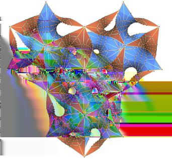
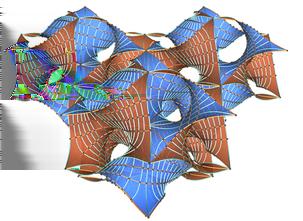
77 4. REVIEW OF KNOWN EXAMPLES 68 Figure The Lidinoid

78 4. REVIEW OF KNOWN EXAMPLES 69 To construct the Lidinoid, let (X, G, dh) be the Weierstraß data describing a member of the rh family. Lidin [FHL93, FH99] gives that the angle of association is approximately θ Furthermore, we expect, as with the gyroid, that the vertical period problem is solved by having the dh flat structure be tipped on end as in the case of the gyroid (see, e.g., 4.7). We can compute the conformal structure of the quotient torus, therefore, as the torus generated by 1 and ai, where (4.57) a = arccot( ) As in the case of the gyroid, we can easily calculate the periods for all members of the associate family by using the H surface flat structures. For instance, one can compute that for all 0 θ 2π, the associate surface has periods: (4.58) (4.59) P (A 1 ) = ( 3p sin(θ), p sin(θ), ) P (B 3 ) = ( 3p sin(θ), p sin(θ), ) These two periods clearly generate the horizontal part of the lattice, so we must ensure the others are compatible. For instance, (4.60) P (B 1 ) = ( 3p sin(θ), (2q + 3p) cos(θ), ) have We see that, since sin(θ) 0 for non-trivial members of the associate family, we must (4.61) (2q + 3p) cos(θ) = sin(θ). Examining the periods for B 2 shows that we must choose the + equation, so that ( 3p 2q ) (4.62) θ = arctan. p Similarly to the gyroid, Equation 4.62 puts a constraint on θ, and the vertical period condition places another condition; these two conditions are compatible for exactly one value of θ the value that gives the Lidinoid.

79 4. REVIEW OF KNOWN EXAMPLES 70 We record here the full set of periods of the Lidinoid for our parameterization: (4.63) (4.64) (4.65) (4.66) (4.67) (4.68) P (A 1 ) = R 2πi (0, 1, 0) 3 P (A 2 ) = R 2πi (0, 1, 0) 3 P (A 3 ) = (0, 0, 3s) P (B 1 ) = R 4πi (0, 1, s) 3 P (B 2 ) = R 4πi (0, 1, s) 3 P (B 3 ) = R 4πi (0, 1, s) 3 where s R + is calculated with an elliptic integral The P Surface from the standpoint of an order 3 symmetry In addition to the order 2 rotational symmetry, the standard, most symmetric P surface also admits an order 3 symmetry. This symmetry permutes the handles of the P surface and is obtained by rotating by 2π 3 though the normal at one of the eight points where the Gaußian curvature K = 0. As discussed in the introduction, these are precisely the hyperelliptic points. The P surface can be viewed as being tiled by right-angled hexagons; the hyperelliptic points are the centers of these hexagons. We repeat the procedure discussed above for the P surface (viewed as invariant under an order 2 rotation), and we obtain again a one-parameter family of P surfaces, this time invariant under an order 3 rotation. The quotient torus is again rectangular (because the surface admits a plane of reflection that commutes with the rotation that has disconnected fixed point sets), the branch points cannot be situated at 0 and 1 2 (since this describes the H surface, as we have already seen). By the discussion in Section 3.1.1, we are forced to place the zero of the Gauß map at 0 and the pole of the Gauß map at τ 2. We illustrate in Figure 4.16 the rather complicated conformal model of the order-3 P surface, showing the branch cuts, the three sheets, and the cycles on the quotient torus. We illustrate in Figure 4.17 the cycles that generate H 1 (P, Z).

80 4. REVIEW OF KNOWN EXAMPLES 71 to 3 to 3 A 1 to 2 to 3 B 2 B 1 to 1 to 1 A 2 to 3 to 1 B 3 B 2 to 2 to 2 A 3 to 1 to 2 B 1 B 3 Figure The conformal structure of the order 3 P surface Flat structures. The 1-forms Gdh, 1 Gdh, and dh each place a flat structure on the torus which, after taking the quotient with id, descends to the sphere. As before, we study each flat structure independently: dh flat structure for the rp D surface. Since the dh flat structure descends as dz, the flat structure for the torus is simply the rectangle Gdh flat structure for the rp D surface. As noted in Section 2.4.2, the order of the zeros and poles of the 1-form Gdh produce cone angles on the torus of 10π 3 i at 0 and of

81 4. REVIEW OF KNOWN EXAMPLES 72 B 2 A 1 Figure Generating cycles for the homology of the order 3 P surface. Notice that, for convenience we have not chosen a standard basis (i.e., B 1 B 2 ). 2π 3 at τ 2. The remaining fixed points, at 1 2 and τ 2, are regular points. The involution id halves the cone angles in the quotient, so that on the sphere the cone angles are: A cone point of angle 10π 6 at 0. A cone point of angle π 3 at τ 2. A cone point of angle π at each of τ 2 and 1 2. The flat structure is a hexagon: Lemma 4.5. By cutting along the shortest geodesics on the sphere from τ 2 to 0, 0 to 1 2, and from 1 2 to τ 2, we obtain a hexagon shown in black in Figure 4.19 (the vertices of the hexagon have labeled coordinates). The hexagon has the following properties: i) the length of l i is equal to the length of l i for i = 1, 2, 3 ii) the angle between l 1 and l 2 and the angle between l 1 and l 2 are both 5π 6. iii) the angle between l 1 and l 1 is π and the angle between l 3 and l 3 is π 6. iv) the angle between l 2 and l 3 and the angle between l 2 and l 3 are both π 2.

82 4. REVIEW OF KNOWN EXAMPLES 73 We again omit the proof, but it is precisely analogous to Lemma 4.1. Again we have not chosen the imaginary part of τ as we expect to recover a family of surfaces Gdh flat structure for the rp D surface. The symmetry between the Gdh and 1 G dh flat structures are now somewhat different, since 1 G (z) and G(z ) do not have the same zeros and poles. Consider instead the maps 1 G (z) and G(z τ 2 ). These have the exactly the same zeros and poles. By Liouville s theorem, G 2 (z + w 1+w 2 2 ) and 1 G 2 (z) are equal up to a complex scalar multiple. Therefore we can understand 1 G in region R (a partial fundamental domain for our developing map) by understanding G in region S (see Figure 4.18). However, under id, R and S are identified, so that, after a relabeling, the development of region R by the Gdh flat structure and the development of R by the 1 Gdh flat structure differ by only a dilation and rigid motion. We adjust ρ to correct this deficiency, and obtain the flat structures shown in Figure S R Figure The shaded regions on the torus are identified under ι The period problem for the rpd surface. Again, we develop the cycles shown in Figure 4.16 and obtain the following periods: (4.69) Gdh = 2i( 3p + q) A 1 1 (4.70) A 1 G dh = 2i( 3p + q) (4.71) Gdh = e 4πi 3 ( 2p 3q + i(2 3p + 3q)) B 1 1 4πi (4.72) dh = e 3 ( p 3pi) B 1 G (4.73) Gdh = e 2πi 3 2i( 3p + q) A 2 1 2πi (4.74) dh = e 3 2i( 3p + q) A 2 G

83 4. REVIEW OF KNOWN EXAMPLES 74 ( p 3q, 3p + q) (p, 3p + q) (p, 3p) ( p 2, 3p 2 ) (0, 0) ( 3 2 q, 1 2 q) Figure Gdh (in black) and 1 Gdh (in blue) flat structures for the P surface viewed as invariant under an order 3 rotation. (4.75) Gdh = 2p 3q + i(2 3p + 3q) B 2 1 (4.76) B 2 G dh = p 3pi (4.77) Gdh = e 4πi 3 2i( 3p + q) A 3 1 4πi (4.78) dh = e 3 2i( 3p + q) A 3 G (4.79) Gdh = e 2πi 3 ( 2p 3q + i(2 3p + 3q)) B 3 1 2πi (4.80) dh = e 3 ( p 3pi) B 3 G

84 4. REVIEW OF KNOWN EXAMPLES 75 (4.81) (4.82) (4.83) (4.84) (4.85) (4.86) P (A 1 ) = (0, 0, 0) P (A 2 ) = (0, 0, 0) P (A 3 ) = (0, 0, 0) P (B 1 ) = R 4πi (p + 3q, 3p 3q, 1) 3 P (B 2 ) = (p + 3q, 3p 3q, 1) P (B 3 ) = R 2πi (p + 3q, 3p 3q, 1) 3 (Again, the notation R 2πi 3 means a rotation by 2πi 3 about the x 3 axis.) The rp D family has one additional feature that we have not seen in the other families: it is self-adjoint. We consider the developed image of the dh flat structure. For the P surface, one of the branch points is at zero (the zero of the Gauß map) and the other is at τ 2 (the pole of the Gauß map). To obtain the conjugate surface, we change dh to e i π 2 dh. This puts the developed image of the branch points at 0 and τ 2. By double periodicity, this is precisely the same developed image as for the P surface (with torus generators swapped). Thus, both the P and D surfaces are in the same family. The CLP surface (below) also shares this characteristic The order 3 gyroid. Since the standard P surface is a member of the rp D family, the gyroid can also be parameterized in terms of this family. We outline the construction of the gyroid in this way, so that in Chapter 5 we can construct (a second) family of gyroids the order 3 gyroids rg. To begin, we need to locate the conformal parameter τ that yields the standard, most symmetric P surface. From the end of Section 4.2, recall that the standard P surface can be described in terms of the 1-forms ω 1, ω 2, and ω 3 (these forms are considered with the orientation of the P surface in space so that the lattice is the standard, cubical lattice). These are permuted by the rotation ρ 3. After a rotation of the surface in space so that the axis of rotation is vertical, dh = ω 1 + ω 2 + ω 3. We understand the periods of these 1-forms

85 4. REVIEW OF KNOWN EXAMPLES 76 Figure Members of the rpd family. The lower right image shows a close up of helicoids forming in the limit. τ = 0.2 τ = 0.45 τ = 1.0 τ = 1.5 τ = 2.5

86 4. REVIEW OF KNOWN EXAMPLES 77 explicitly from our work with the P surface. Denote by γ 1 the cycle generated by the vector 1 on the order 2 P surface torus. Its period on each of the ω i flat structures is 1, i.e., (4.87) ω i = 1 γ 1 so that (4.88) dh = γ 1 ω 1 + ω 2 + ω 3 = 1 γ 1 This implies that one generator of the quotient torus P/ρ 3 is 1, since the location of the branch cuts implies that this cycle γ 1 continues onto all three sheets. Considering the other generator of the torus (rather, the cycle γ 2 coinciding with this generator), we note that (4.89) ω i = 2a γ 2 since the cycle continues onto both sheets of the torus P/ρ 2 (recall that a = Im τ 0.78). On the other hand, if we denote the generators of the torus P/ρ 3 by 1 and σ, then (4.90) dh = γ 2 ω 1 + ω 2 + ω 3 = 6a γ 2 but also (4.91) dh = 3 Im σ γ 2 since the cycles continues onto both sheets. Thus, the standard P surface is obtained when σ = 2τ. Since this is the standard P surface, the angle of association that yields the gyroid is the same (4.92) θ = arccot Im τ We remark that this is precisely the same surface as that obtain in Section 4.2, but viewed from a different perspective and using a different parameterization. Another view of the gyroid is in Figure 4.21.

87 4. REVIEW OF KNOWN EXAMPLES 78 Figure Top: a translational fundamental domain of the gyroid, viewed as invariant under an order 3 rotation. Bottom: several copies of a fundamental domain. Notice the similarity to the Lidinoid The CLP surface Another classical surface, the CLP surface (for crossed layers of parallels ), is shown in Figure This genus 3 surface also admits an order 2 rotation with four fixed points.

88 4. REVIEW OF KNOWN EXAMPLES 79 Figure A fundamental domain for the CLP surface The quotient torus is rectangular (again, by symmetry considerations); Figure 4.25 shows the conformal model. Figure 4.24 shows a schematic view of the CLP surface with cycles illustrated Flat structures and periods for the CLP surface. As in the case of the P and H surfaces, G 2( z + 2) 1 ( and 1 2(z) G) have precisely the same zeros and poles to the same order. Again, by Liouville s theorem, the quotient is constant (since it is holomorphic (no poles) and doubly periodic): ( (4.93) G 2 z + 1 ) ( ) (z) = r 1 e iφ 1 2 G By adjusting the Lopez-Ros parameter, we can ensure that this factor is 1, and we do that for the CLP surface. Therefore, the 1 Gdh flat structure is simply a translation of the (infinite, periodic) Gdh flat structure. This is reflected in the blue outline of the 1 Gdh flat structure in Figure 4.26.

89 4. REVIEW OF KNOWN EXAMPLES 80 Figure Several fundamental domains of CLP Figure Alternate view of the CLP surface, showing the cycles. B 3 B1 A 1 A3 A 2 B 2

90 4. REVIEW OF KNOWN EXAMPLES 81 A 2 B 1 A 1 B 2 A 3 B 3 Figure The quotient torus M/ρ for the surface M = CLP, showing the location of the branch points and the six generators of the homology. A conformal model for the full surface is obtained by gluing along the indicated branch cuts (in red). ( p, p + q) (p, p + q) ( p, p) (p, p) (0, q) (0, 0) Figure The Gdh (in black) and 1 Gdh (in blue) flat structures for the CLP surface. Labeled vertices are for the Gdh flat structure (the corresponding points on 1 Gdh are obtained by translation by ( p, p).

91 4. REVIEW OF KNOWN EXAMPLES 82 We now calculate the periods for the CLP surface; we have omitted the calculation for A 3 since the period is always 0 under the order 2 assumption. (4.94) Gdh = (1 i)(p + p i) A 1 (4.95) 1 dh = (1 + i)(p p i) A 1 G (4.96) Gdh = (1 i)qi B 1 (4.97) 1 dh = (1 + i)qi B 1 G (4.98) Gdh = (1 i)(p p i) A 2 (4.99) 1 dh = (1 + i)(p + p i) A 2 G (4.100) Gdh = (1 + i)qi B 2 (4.101) 1 dh = (1 i)qi B 2 G (4.102) (4.103) Gdh = 2p B 3 1 dh = 2p B 3 G (4.104) (4.105) (4.106) (4.107) (4.108) (4.109) P (A 1 ) = (0, 0, 0) P (A 2 ) = (0, 0, 0) P (A 3 ) = (0, 0, 0) P (B 1 ) = ( 2q, 2q, 0) P (B 2 ) = (2q, 2q, 0) P (B 3 ) = (0, 0, 1) There are no known embedded members of the associate family of any surface in the tclp family.

92 4. REVIEW OF KNOWN EXAMPLES 83 Figure The tclp deformation of the CLP surface. τ = 0.2 τ = 0.6 τ = 0.9 τ = 1.5 τ = 2.0 τ = 4.0