Methodological workshop How to get it right: why you should think twice before planning your next study. Part 1
|
|
|
- Georgia Nichols
- 5 years ago
- Views:
Transcription


1 Methodological workshop How to get it right: why you should think twice before planning your next study Luigi Lombardi Dept. of Psychology and Cognitive Science, University of Trento Part 1
2 1 The power algebra
3 1 The power algebra The Neyman-Pearson paradigm (N-H)
4 1 The power algebra
5 1 The power algebra power The N-H table
6 1 The power algebra Probabilistic interpretation

7 1 The power algebra Graphical interpretation
8 1 The power algebra Decision rule in the N-H approach
9 1 The power algebra Power analysis is based on four different parameters: Power (population level) Hypothetical Sample size Type I error (population level) Effect size (population level)

10 1 The power algebra Effect size parameter defining HA; it represents the degree of deviation from H0 in the underlying population Effect size (population level)

11 1 The power algebra A priori power analysis
12 1 The power algebra A priori power analysis: an example using the pwr package One-sample t-test: H pwr.t.test(d=0.2,power=0.85,sig.level=0.05,n=null,typ e="one.sample",alternative="greater") R syntax One-sample t test power calculation n = d = 0.2 sig.level = 0.05 power = 0.85 alternative = greater R output

13 1 The power algebra Post hoc power analysis
 R syntax One-sample t test power calculation 0.454 n = 60 d = 0.2 sig.level = 0.05 power = 0.")
14 1 The power algebra Post hoc power analysis: an example using the pwr package One-sample t-test: H pwr.t.test(d=0.2,n=60,sig.level=0.05,power=null,type= "one.sample",alternative="greater") R syntax One-sample t test power calculation n = 60 d = 0.2 sig.level = 0.05 power = alternative = greater R output

15 1 The power algebra Sensitivity analysis.
16 1 The power algebra Sensitivity analysis: an example using the pwr package One-sample t-test: H pwr.t.test(n=50,power=0.9,sig.level=0.05,d=null,type= "one.sample",alternative="greater") R syntax One-sample t test power calculation n = 50 d = sig.level = 0.05 power = 0.9 alternative = greater R output
17 1 The power algebra Criterion analysis.
18 1 The power algebra Criterion analysis: an example using the pwr package One-sample t-test: H pwr.t.test(n=100,d=0.3,power=0.9,sig.level=null,type= "one.sample",alternative="greater") R syntax One-sample t test power calculation n = 100 d = 0.3 sig.level = power = 0.9 alternative = greater R output

19 1 The power algebra: the power fallacy.
20 1 The power algebra: the power fallacy Observed power analysis The basic idea of observed power analysis is that there is evidence for the null hypothesis being true if p > and the computed power is high at the observed effect size d The effect size (at population level) is replaced with the observed effect size d (at the sample level)
21 1 The power algebra: the power fallacy Observed power analysis The effect size (at population level) is replaced with the observed effect size d (at the sample level) Note d is not a theoretical value (hypothetical value)
22 1 The power algebra: the power fallacy Observed power analysis The effect size (at population level) is replaced with the observed effect size d (at the sample level) Note d is not a theoretical value (hypothetical value) It is estimated from the sample according to the theoretical model for the null hypothesis
23 1 The power algebra: the power fallacy Observed power analysis The effect size (at population level) is replaced with the observed effect size d (at the sample level) Note d is not a theoretical value (hypothetical value) It is estimated from the sample according to the theoretical model for the null hypothesis It is biased!!!
 AND (power is high)] iff NOT(p > ) OR NOT(power is high) Some derivations : 1. NOT(p > ) AND (power is high) entails?? 2. (p > ) AND NOT(power is high) entails?? 3.")
24 1 The power algebra: the power fallacy Observed power analysis hypothetical derivations Basic power analysis claim: (p > ) AND (power is high) entails «evidence for H0 is high» Some derivations : NOT [(p > ) AND (power is high)] iff NOT(p > ) OR NOT(power is high) Some derivations : 1. NOT(p > ) AND (power is high) entails?? 2. (p > ) AND NOT(power is high) entails?? 3. NOT(p > ) AND NOT(power is high) entails??
25 1 The power algebra: the power fallacy Observed power analysis hypothetical derivations Some interpretations: (p > ) AND NOT(power is high) entails «evidence for H0 is weak» The underlying idea is: if we increase the sample size, then we raise the power, and probably we can reject H0! However some of these interpretations lead us to the a paradox!
26 1 The power algebra: the power fallacy There is a negative monotonic relationship between observed power and p-value!
27 1 The power algebra: the power fallacy That is to say, because of the one-to-one relationship between p-values and observed power, nonsignificant p-values always correspond to low observed powers!!! There is a negative monotonic relationship between observed power and p-value!

28 1 The power algebra: the power fallacy That is to say, because of the one-to-one relationship between p-values and observed power, nonsignificant p-values always correspond to low observed powers!!! Hence, we will never observe nonsignificant p-values corresponding to high observed powers. The main claim is a nonsense! There is a negative monotonic relationship between observed power and p-value!
29 1 The power algebra: the power fallacy relationship between observed power and p-value simulation study
)/sqrt(((n-1)*sd^2)/(n-1)) simpv[b] <- t.test(x)$p.value simpw[b] <- pwr.t.test(d=dobs,n=n,sig.level=0.05,power=null, type=\"one.sample\",alternative=\"two.")
30 1 The power algebra: the power fallacy One-sample t-test: H0 0 = 0 (simulation study) n <- 50 mu0 <- 0 sd <- 1 B < simpv <- rep(0,b) simpw <- rep(0,b) for (b in 1:B) { } X <- rnorm(n,mu0,sd) dobs <- (mean(x))/sqrt(((n-1)*sd^2)/(n-1)) simpv[b] <- t.test(x)$p.value simpw[b] <- pwr.t.test(d=dobs,n=n,sig.level=0.05,power=null, type="one.sample",alternative="two.sided")$power plot(simpv,simpw,ylab="observed power", xlab="p-value") R syntax
31 2 Computing observed effect sizes

32 2 Computing observed effect sizes Observed effect sizes allow to compute the magnitute of an effect of interest. They can be understood as estimates of the differences between groups or the strength of associations between variables. Widely used examples of observed effect sizes are: Different typologies of d measures (Cohen, 1988; Hedges, 1981; Rosenthal, 1994; Dunlap et al., 1996) Association measures such as, for example, the correlation r Differences Between groups Association between quantitative variables


33 2 Computing observed effect sizes Observed effect size for comparing two independent groups

34 2 Computing observed effect sizes Observed effect size for comparing two independent groups with t values Note this is a Transformation index


35 2 Computing observed effect sizes Observed effect size for comparing two dependent groups with t values

36 2 Computing observed effect sizes Conversion formulae Note however that conversions may unnecessarily incur in some sort of bias
 of a categorical predictor variable (specifically for each of its recoded dummy variables of the categorical predictor): Categorical predictor Continuous")
37 2 Computing observed effect sizes Observed effect size derived from regression models In general, it is always possible to obtain t values from a regression model for each continuous predictor variable and also for each group (level) of a categorical predictor variable (specifically for each of its recoded dummy variables of the categorical predictor): Categorical predictor Continuous predictor where n1 and n2 are the sample sizes for two groups and df denotes the degrees of freedom used for the associated t value in a linear model

38 2 Computing observed effect sizes Deriving approximate confidence intervals (CI) for effect sizes In general, computing approximate CI for effect sizes is not an easy task as the equations usually vary according to the selected effect size index and also the way it has been derived from the specific statistical analysis. A general equation is the following: 95% CI for ES The main problem regards the way we compute the asymptotic standard error (se). A better way may be to use a parametric bootstrap approach to derive empirical Cis for effect sizes.
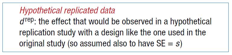
 a <- c(rep(\"a1\",n/2),rep(\"a2\",n/2)) x2 <- c(rep(0,n/2),rep(1,n/2)) y <- beta0 + beta1*x1 + beta2*x2 + rnorm(n,0,4) plot(x1,y) plot(x2,y) boxplot(y ~ a) MR <- lm(y ~ x1")
39 2 Computing observed effect sizes Multiple regression model: 1 quant. predictor + 1 categ. predictor (simulation study) beta0 <- 0 beta1 < beta2 < n <- 100 x1 <- rnorm(n,10,5) a <- c(rep("a1",n/2),rep("a2",n/2)) x2 <- c(rep(0,n/2),rep(1,n/2)) y <- beta0 + beta1*x1 + beta2*x2 + rnorm(n,0,4) plot(x1,y) plot(x2,y) boxplot(y ~ a) MR <- lm(y ~ x1 + a) summary(mr) # effect size categorical variable a - second level (a2) d <- (summary(mr)$coefficients[3,3]*(n))/(sqrt((n/2)^2)*sqrt(mr$df)) # effect size for the quantitative variable x1 r <- summary(mr)$coefficients[2,3]/sqrt(summary(mr)$coefficients[2,3]^2 + MR$df) d r R syntax ( )
![# Parametric bootstrap for approximate 95% CIs for effect sizes ##### # number of simulations: B B <- 500 dsim <- rep(0,b) rsim <- rep(0,b) for (b in 1:B) { YS <- simulate(mr,1)[,1] MS <- lm(ys ~ x1](/docs-images/96/126524744/images/40-1.jpg "+ a) # absolute effect size dsim[b] <- abs(summary(ms)$coefficients[3,3]*(n))/(sqrt((n/2)^2)*sqrt(ms$df)) rsim[b] <- summary(ms)$coefficients[2,3]/sqrt(summary(ms)$coefficients[2,3]^2 + MS$df) }")
40 # Parametric bootstrap for approximate 95% CIs for effect sizes ##### # number of simulations: B B <- 500 dsim <- rep(0,b) rsim <- rep(0,b) for (b in 1:B) { YS <- simulate(mr,1)[,1] MS <- lm(ys ~ x1 + a) # absolute effect size dsim[b] <- abs(summary(ms)$coefficients[3,3]*(n))/(sqrt((n/2)^2)*sqrt(ms$df)) rsim[b] <- summary(ms)$coefficients[2,3]/sqrt(summary(ms)$coefficients[2,3]^2 + MS$df) } par(mfrow=c(1,2)) plot(density(dsim),main="distribution for simulated d ") hist(dsim,freq=f,add=t) plot(density(rsim),main="distribution for simulated r") hist(rsim,freq=f,add=t) quantile(dsim,probs=c(0.025,0.975)) quantile(rsim,probs=c(0.025,0.975)) R syntax (end) Multiple regression model: 1 quant. predictor + 1 categ. predictor (simulation study) 1
 95% CI for d [0.508, 1.")
41 1 Multiple regression model: 1 quant. predictor + 1 categ. predictor (simulation study) 95% CI for d [0.508, 1.357] 95% CI for r [0.368, 0.654]
 a <- c(rep(\"a1\",n/2),rep(\"a2\",n/2)) x2 <- c(rep(0,n/2),rep(1,n/2)) mul <- beta0 + beta1*x1 + beta2*x2 # linear predictor pis <- exp(mul)/(1+exp(mul)) # inverse")
42 2 Multiple logistic regression model: 1 quant. predictor + 1 categ. predictor (simulation study) beta0 <- 0 beta1 <- 0.5 beta2 < n <- 100 x1 <- rnorm(n,10,5) a <- c(rep("a1",n/2),rep("a2",n/2)) x2 <- c(rep(0,n/2),rep(1,n/2)) mul <- beta0 + beta1*x1 + beta2*x2 # linear predictor pis <- exp(mul)/(1+exp(mul)) # inverse transformation mul y <- rbinom(n,40,pis) # generate binomial counts u.b. = 40 plot(x1[a=="a1"],y[a=="a1"],xlab="x1",ylab="y") points(x1[a=="a2"],y[a=="a2"],pch=3) MR <- glm(cbind(y,40-y) ~ x1 + a, family='binomial') summary(mr) df <- 97 # as if t-tests were used # effect size categorical variable a - second level (a2) d <- (summary(mr)$coefficients[3,3]*(n))/(sqrt((n/2)^2)*sqrt(df)) # effect size for the quantitative variable x1 r <- summary(mr)$coefficients[2,3]/sqrt(summary(mr)$coefficients[2,3]^2 + df) d r R syntax ( )
43 2 Multiple logistic regression model: 1 quant. predictor + 1 categ. predictor (simulation study) # Parametric bootstrap for approximate 95% CIs for effect sizes ##### B <- 500 dsim <- rep(0,b) rsim <- rep(0,b) for (b in 1:B) { YS <- simulate(mr,1)[,1] MS <- glm(ys ~ x1 + a, family='binomial') # absolute effect size dsim[b] <- abs(summary(ms)$coefficients[3,3]*(n))/(sqrt((n/2)^2)*sqrt(df)) rsim[b] <- summary(ms)$coefficients[2,3]/sqrt(summary(ms)$coefficients[2,3]^2 + df) } par(mfrow=c(1,2)) plot(density(dsim),main="distribution for simulated d ") hist(dsim,freq=f,add=t) plot(density(rsim),main="distribution for simulated r") hist(rsim,freq=f,add=t) quantile(dsim,probs=c(0.025,0.975)) quantile(rsim,probs=c(0.025,0.975)) R syntax (end)
44 2 Multiple logistic regression model: 1 quant. predictor + 1 categ. predictor (simulation study) 95% CI for d [2.318, 2.767] 95% CI for r [0.908, 0.917]
 z Categorical predictor Continuous predictor For glm (generalized linear models) the t values must be replaced with z values.")
45 2 Multiple logistic regression model: 1 quant. predictor + 1 categ. predictor (simulation study) z Categorical predictor Continuous predictor For glm (generalized linear models) the t values must be replaced with z values. However, the degrees of freedom should be computed as if t- tests were used. Cautionary note When using glm models to derive ESs, it is uncertain the amount of bias that may be incurred using the above modified equations
46 3 Beyond power calculations

47 3 Beyond power calculations One of the main problems of standard power analysis is that it puts a narrow emphasis on statistical significance which is the primary focus of many study designs. However, in noisy, small-sample settings, statistically significant results can often be misleading. This is particularly true when observed power analysis is used to evaluate the statistical results.
48 3 Beyond power calculations A better approach would be Design Analysis (DA): a set of statistical calculations about what could happen under hypothetical replications of a study (that focuses on estimates and uncertainties rather than on statistical significance)

49 3 Beyond power calculations Somehow this work represents a kind of conceptual «bridge» linking the frequentist approach with a more Bayesian oriented perspective
50 3 Beyond power calculations DA main tokens The observed effect The true population effect The standard error (SE) of the observed effect The Type I error A hypothetical normally distributed random variable with parameters D and s (note this constitutes a conceptual leap)

51 3 Beyond power calculations DA main tokens The main goals are to compute: and dc being the cumulative standard normal distribution and the critical value for the effect size, respectively
52 3 Beyond power calculations DA main tokens The main goals are to compute:

53 3 Beyond power calculations DA main tokens The main goals are to compute:


54 3 Beyond power calculations Gelman & Carlin (2014), p. 644

55 3 Beyond power calculations retrodesign <- function(a, s, alpha=.05, df=inf, n.sims=10000){ z <- qt(1-alpha/2, df) p.hi <- 1 - pt(z-a/s, df) p.lo <- pt(-z-a/s, df) power <- p.hi + p.lo types <- p.lo/power estimate <- A + s*rt(n.sims,df) significant <- abs(estimate) > s*z exaggeration <- mean(abs(estimate)[significant])/a return(list(power=power,types=types,exaggeration=exaggeration)) } R function: Gelman & Carlin (2014), p. 644
56 3 Beyond power calculations A simple example: linear regression
 (Intercept) -0.6061 3.9588-0.153 0.879 x 2.1792 0.3697 5.894 7.96e-07 *** --- Signif. codes: 0 *** 0.001 ** 0.01 * 0.05. 0.1 1 Residual standard error: 7.")
57 3 Beyond power calculations Call: lm(formula = y ~ x) Simple regression with lm() Residuals: Min 1Q Median 3Q Max Coefficients: Estimate Std. Error t value Pr(> t ) (Intercept) x e-07 *** --- Signif. codes: 0 *** ** 0.01 * Residual standard error: on 38 degrees of freedom Multiple R-squared: , Adjusted R-squared: F-statistic: on 1 and 38 DF, p-value: 7.955e-07 R syntax
![3 Beyond power calculations > retrodesign(1, 0.3697, df=38) $power [1] 0.](/docs-images/96/126524744/images/58-1.jpg "7498592 $types [1] 2.054527e-05 $exaggeration [1] 1.")
58 3 Beyond power calculations > retrodesign(1, , df=38) $power [1] $types [1] e-05 $exaggeration [1] Design Analysis D = 1 True population effect R syntax
59 3 Beyond power calculations D = 1
![3 Beyond power calculations > retrodesign(0.5, 0.3697, df=38) $power [1] 0.](/docs-images/96/126524744/images/60-1.jpg "2536931 $types [1] 0.003356801 Design Analysis D = 0.")
60 3 Beyond power calculations > retrodesign(0.5, , df=38) $power [1] $types [1] Design Analysis D = 0.5 True population effect $exaggeration [1] R syntax
61 3 Beyond power calculations D = 0.5
 : 39.")
62 3 Beyond power calculations 5000 simulated samples with 20 observations each from a normal distribution with parameters = 0.5; s = 0.9 % of significant results ( 0) : 39.7 % of sample means > D(= ) : 32.3
63 3 Beyond power calculations Type S error as a function of Power Gelman & Carlin (2014), p. 644
64 3 Beyond power calculations Exaggeration ratio as a function of Power Gelman & Carlin (2014), p. 644
 may really be a loss (in the form of a claim that does not")
65 3 Beyond power calculations Practical implications: Design Analysis strongly suggest larger sample sizes than those that are commonly used in psychology. In particular, if sample size is too small, in relation to the true effect size, then what appears to be a win (statistical significance) may really be a loss (in the form of a claim that does not replicate). For a more formal presentation of the DA approach see Gelman A. & Tuerlinckx F. (2000). Type S error rates for classical and Bayesian single and multiple comparison procedures. Computational Statistics, 15,
66 4 Fake data analysis
 SGR is a data simulation procedure that allows to generate artificial samples of fake discrete/ordinal data.")

67 4 Fake data analysis: the SGR approach SGR = Sample Generation by Replacement (Lombardi & Pastore, 2012; Pastore & Lombardi, 2014, Lombardi & Pastore, 2014; Lombardi et al., 2015) SGR is a data simulation procedure that allows to generate artificial samples of fake discrete/ordinal data. SGR can be used to quantify uncertainty in inferences based on possible fake data as well as to evaluate the implications of fake data for statistical results. For example, how sensitive are the results to possible fake data? Are the conclusions still valid under one or more scenarios of faking manipulations?

68 4 Fake data analysis: the SGR approach Some «examples»

69 4 Fake data analysis: the SGR approach Some «examples»
70 4 Fake data analysis: the SGR approach The SGR logic
71 4 Fake data analysis: the SGR approach The SGR logic This is usually not directly observable This is observable Information (data)

72 Original value d 4 Fake data analysis: the SGR approach The replacement distribution Replaced value f
73 4 Fake data analysis: the SGR approach Other examples of replacement distribution

74 4 Fake data analysis: the SGR approach Other examples of replacement distribution
75 4 Fake data analysis: the SGR approach The sgr package (The R Journal, 6(1), )
, 164-177) sgr package is available on the CRAN")
76 4 Fake data analysis: the SGR approach The sgr package (The R Journal, 6(1), ) sgr package is available on the CRAN repository
77 Spearman correlation 4 Fake data analysis: the SGR approach Effect of faking on two items that are originally not correlated (n=50) Proportion of subjects with fake responses (faking-good type)
78 Spearman correlation 4 Fake data analysis: the SGR approach Effect of faking on two items that are originally not correlated (n=100) Proportion of subjects with fake responses (faking-good type)
79 4 Fake data analysis: the SGR approach SGR allows to test and compare different fake data models Fake data hypotheses

80 4 Fake data analysis: the SGR approach SGR allows to test and compare different fake data models
81 4 Fake data analysis: the SGR approach SGR allows to test and compare different fake data models also more complex factorial models
82 4 Fake data analysis: the SGR approach SGR allows to test and compare different fake data models to evaluate the effect on g.o.f. statistics

83 Thank you for your attention! visit the WS website at
7.2 One-Sample Correlation ( = a) Introduction. Correlation analysis measures the strength and direction of association between
 Introduction. Correlation analysis measures the strength and direction of association between") 7.2 One-Sample Correlation ( = a) Introduction Correlation analysis measures the strength and direction of association between variables. In this chapter we will test whether the population correlation
7.2 One-Sample Correlation ( = a) Introduction Correlation analysis measures the strength and direction of association between variables. In this chapter we will test whether the population correlation
Hypothesis Testing. Part I. James J. Heckman University of Chicago. Econ 312 This draft, April 20, 2006
 Hypothesis Testing Part I James J. Heckman University of Chicago Econ 312 This draft, April 20, 2006 1 1 A Brief Review of Hypothesis Testing and Its Uses values and pure significance tests (R.A. Fisher)
Contents. Acknowledgments. xix
 Table of Preface Acknowledgments page xv xix 1 Introduction 1 The Role of the Computer in Data Analysis 1 Statistics: Descriptive and Inferential 2 Variables and Constants 3 The Measurement of Variables
Linear Regression. In this lecture we will study a particular type of regression model: the linear regression model
 1 Linear Regression 2 Linear Regression In this lecture we will study a particular type of regression model: the linear regression model We will first consider the case of the model with one predictor
Workshop 7.4a: Single factor ANOVA
 -1- Workshop 7.4a: Single factor ANOVA Murray Logan November 23, 2016 Table of contents 1 Revision 1 2 Anova Parameterization 2 3 Partitioning of variance (ANOVA) 10 4 Worked Examples 13 1. Revision 1.1.
Business Statistics. Lecture 10: Course Review
 Business Statistics Lecture 10: Course Review 1 Descriptive Statistics for Continuous Data Numerical Summaries Location: mean, median Spread or variability: variance, standard deviation, range, percentiles,
1. Hypothesis testing through analysis of deviance. 3. Model & variable selection - stepwise aproaches
 Sta 216, Lecture 4 Last Time: Logistic regression example, existence/uniqueness of MLEs Today s Class: 1. Hypothesis testing through analysis of deviance 2. Standard errors & confidence intervals 3. Model
1 The Classic Bivariate Least Squares Model
 Review of Bivariate Linear Regression Contents 1 The Classic Bivariate Least Squares Model 1 1.1 The Setup............................... 1 1.2 An Example Predicting Kids IQ................. 1 2 Evaluating
3 Joint Distributions 71
 2.2.3 The Normal Distribution 54 2.2.4 The Beta Density 58 2.3 Functions of a Random Variable 58 2.4 Concluding Remarks 64 2.5 Problems 64 3 Joint Distributions 71 3.1 Introduction 71 3.2 Discrete Random
Subject CS1 Actuarial Statistics 1 Core Principles
 Institute of Actuaries of India Subject CS1 Actuarial Statistics 1 Core Principles For 2019 Examinations Aim The aim of the Actuarial Statistics 1 subject is to provide a grounding in mathematical and
Stat 401B Final Exam Fall 2015
 Stat 401B Final Exam Fall 015 I have neither given nor received unauthorized assistance on this exam. Name Signed Date Name Printed ATTENTION! Incorrect numerical answers unaccompanied by supporting reasoning
Biostatistics for physicists fall Correlation Linear regression Analysis of variance
 Biostatistics for physicists fall 2015 Correlation Linear regression Analysis of variance Correlation Example: Antibody level on 38 newborns and their mothers There is a positive correlation in antibody
Stat 5102 Final Exam May 14, 2015
 Stat 5102 Final Exam May 14, 2015 Name Student ID The exam is closed book and closed notes. You may use three 8 1 11 2 sheets of paper with formulas, etc. You may also use the handouts on brand name distributions
Model Selection in GLMs. (should be able to implement frequentist GLM analyses!) Today: standard frequentist methods for model selection
 Today: standard frequentist methods for model selection") Model Selection in GLMs Last class: estimability/identifiability, analysis of deviance, standard errors & confidence intervals (should be able to implement frequentist GLM analyses!) Today: standard frequentist
Model Selection in GLMs Last class: estimability/identifiability, analysis of deviance, standard errors & confidence intervals (should be able to implement frequentist GLM analyses!) Today: standard frequentist
Generalised linear models. Response variable can take a number of different formats
 Generalised linear models Response variable can take a number of different formats Structure Limitations of linear models and GLM theory GLM for count data GLM for presence \ absence data GLM for proportion
MATH 644: Regression Analysis Methods
 MATH 644: Regression Analysis Methods FINAL EXAM Fall, 2012 INSTRUCTIONS TO STUDENTS: 1. This test contains SIX questions. It comprises ELEVEN printed pages. 2. Answer ALL questions for a total of 100
Regression and the 2-Sample t
 Regression and the 2-Sample t James H. Steiger Department of Psychology and Human Development Vanderbilt University James H. Steiger (Vanderbilt University) Regression and the 2-Sample t 1 / 44 Regression
Stat 5101 Lecture Notes
 Stat 5101 Lecture Notes Charles J. Geyer Copyright 1998, 1999, 2000, 2001 by Charles J. Geyer May 7, 2001 ii Stat 5101 (Geyer) Course Notes Contents 1 Random Variables and Change of Variables 1 1.1 Random
Extensions of One-Way ANOVA.
 Extensions of One-Way ANOVA http://www.pelagicos.net/classes_biometry_fa18.htm What do I want You to Know What are two main limitations of ANOVA? What two approaches can follow a significant ANOVA? How
Nature vs. nurture? Lecture 18 - Regression: Inference, Outliers, and Intervals. Regression Output. Conditions for inference.
 Understanding regression output from software Nature vs. nurture? Lecture 18 - Regression: Inference, Outliers, and Intervals In 1966 Cyril Burt published a paper called The genetic determination of differences
Stat/F&W Ecol/Hort 572 Review Points Ané, Spring 2010
 1 Linear models Y = Xβ + ɛ with ɛ N (0, σ 2 e) or Y N (Xβ, σ 2 e) where the model matrix X contains the information on predictors and β includes all coefficients (intercept, slope(s) etc.). 1. Number of
Extensions of One-Way ANOVA.
 Extensions of One-Way ANOVA http://www.pelagicos.net/classes_biometry_fa17.htm What do I want You to Know What are two main limitations of ANOVA? What two approaches can follow a significant ANOVA? How
Final Exam. Name: Solution:
 Final Exam. Name: Instructions. Answer all questions on the exam. Open books, open notes, but no electronic devices. The first 13 problems are worth 5 points each. The rest are worth 1 point each. HW1.
Statistics 572 Semester Review
 Statistics 572 Semester Review Final Exam Information: The final exam is Friday, May 16, 10:05-12:05, in Social Science 6104. The format will be 8 True/False and explains questions (3 pts. each/ 24 pts.
Exam details. Final Review Session. Things to Review
 Exam details Final Review Session Short answer, similar to book problems Formulae and tables will be given You CAN use a calculator Date and Time: Dec. 7, 006, 1-1:30 pm Location: Osborne Centre, Unit
Supplemental Resource: Brain and Cognitive Sciences Statistics & Visualization for Data Analysis & Inference January (IAP) 2009
 2009") MIT OpenCourseWare http://ocw.mit.edu Supplemental Resource: Brain and Cognitive Sciences Statistics & Visualization for Data Analysis & Inference January (IAP) 2009 For information about citing these
MIT OpenCourseWare http://ocw.mit.edu Supplemental Resource: Brain and Cognitive Sciences Statistics & Visualization for Data Analysis & Inference January (IAP) 2009 For information about citing these
Biostatistics 380 Multiple Regression 1. Multiple Regression
 Biostatistics 0 Multiple Regression ORIGIN 0 Multiple Regression Multiple Regression is an extension of the technique of linear regression to describe the relationship between a single dependent (response)
Glossary. The ISI glossary of statistical terms provides definitions in a number of different languages:
 Glossary The ISI glossary of statistical terms provides definitions in a number of different languages: http://isi.cbs.nl/glossary/index.htm Adjusted r 2 Adjusted R squared measures the proportion of the
Swarthmore Honors Exam 2012: Statistics
 Swarthmore Honors Exam 2012: Statistics 1 Swarthmore Honors Exam 2012: Statistics John W. Emerson, Yale University NAME: Instructions: This is a closed-book three-hour exam having six questions. You may
Preview from Notesale.co.uk Page 3 of 63
 Stem-and-leaf diagram - vertical numbers on far left represent the 10s, numbers right of the line represent the 1s The mean should not be used if there are extreme scores, or for ranks and categories Unbiased
Tests of Linear Restrictions
 Tests of Linear Restrictions 1. Linear Restricted in Regression Models In this tutorial, we consider tests on general linear restrictions on regression coefficients. In other tutorials, we examine some
BMI 541/699 Lecture 22
 BMI 541/699 Lecture 22 Where we are: 1. Introduction and Experimental Design 2. Exploratory Data Analysis 3. Probability 4. T-based methods for continous variables 5. Power and sample size for t-based
STAT 3022 Spring 2007
 Simple Linear Regression Example These commands reproduce what we did in class. You should enter these in R and see what they do. Start by typing > set.seed(42) to reset the random number generator so
" M A #M B. Standard deviation of the population (Greek lowercase letter sigma) σ 2
 σ 2") Notation and Equations for Final Exam Symbol Definition X The variable we measure in a scientific study n The size of the sample N The size of the population M The mean of the sample µ The mean of the
Notation and Equations for Final Exam Symbol Definition X The variable we measure in a scientific study n The size of the sample N The size of the population M The mean of the sample µ The mean of the
ST430 Exam 2 Solutions
 ST430 Exam 2 Solutions Date: November 9, 2015 Name: Guideline: You may use one-page (front and back of a standard A4 paper) of notes. No laptop or textbook are permitted but you may use a calculator. Giving
Deciding, Estimating, Computing, Checking
 Deciding, Estimating, Computing, Checking How are Bayesian posteriors used, computed and validated? Fundamentalist Bayes: The posterior is ALL knowledge you have about the state Use in decision making:
Deciding, Estimating, Computing, Checking. How are Bayesian posteriors used, computed and validated?
 Deciding, Estimating, Computing, Checking How are Bayesian posteriors used, computed and validated? Fundamentalist Bayes: The posterior is ALL knowledge you have about the state Use in decision making:
Review: what is a linear model. Y = β 0 + β 1 X 1 + β 2 X 2 + A model of the following form:
 Outline for today What is a generalized linear model Linear predictors and link functions Example: fit a constant (the proportion) Analysis of deviance table Example: fit dose-response data using logistic
Simple, Marginal, and Interaction Effects in General Linear Models
 Simple, Marginal, and Interaction Effects in General Linear Models PRE 905: Multivariate Analysis Lecture 3 Today s Class Centering and Coding Predictors Interpreting Parameters in the Model for the Means
Review of Statistics 101
 Review of Statistics 101 We review some important themes from the course 1. Introduction Statistics- Set of methods for collecting/analyzing data (the art and science of learning from data). Provides methods
Variance. Standard deviation VAR = = value. Unbiased SD = SD = 10/23/2011. Functional Connectivity Correlation and Regression.
 10/3/011 Functional Connectivity Correlation and Regression Variance VAR = Standard deviation Standard deviation SD = Unbiased SD = 1 10/3/011 Standard error Confidence interval SE = CI = = t value for
DESIGNING EXPERIMENTS AND ANALYZING DATA A Model Comparison Perspective
 DESIGNING EXPERIMENTS AND ANALYZING DATA A Model Comparison Perspective Second Edition Scott E. Maxwell Uniuersity of Notre Dame Harold D. Delaney Uniuersity of New Mexico J,t{,.?; LAWRENCE ERLBAUM ASSOCIATES,
Correlation and Simple Linear Regression
 Correlation and Simple Linear Regression Sasivimol Rattanasiri, Ph.D Section for Clinical Epidemiology and Biostatistics Ramathibodi Hospital, Mahidol University E-mail: sasivimol.rat@mahidol.ac.th 1 Outline
Glossary for the Triola Statistics Series
 Glossary for the Triola Statistics Series Absolute deviation The measure of variation equal to the sum of the deviations of each value from the mean, divided by the number of values Acceptance sampling
Sleep data, two drugs Ch13.xls
 Model Based Statistics in Biology. Part IV. The General Linear Mixed Model.. Chapter 13.3 Fixed*Random Effects (Paired t-test) ReCap. Part I (Chapters 1,2,3,4), Part II (Ch 5, 6, 7) ReCap Part III (Ch
Course Introduction and Overview Descriptive Statistics Conceptualizations of Variance Review of the General Linear Model
 Course Introduction and Overview Descriptive Statistics Conceptualizations of Variance Review of the General Linear Model EPSY 905: Multivariate Analysis Lecture 1 20 January 2016 EPSY 905: Lecture 1 -
Statistical. Psychology
 SEVENTH у *i km m it* & П SB Й EDITION Statistical M e t h o d s for Psychology D a v i d C. Howell University of Vermont ; \ WADSWORTH f% CENGAGE Learning* Australia Biaall apan Korea Меяко Singapore
Introduction and Descriptive Statistics p. 1 Introduction to Statistics p. 3 Statistics, Science, and Observations p. 5 Populations and Samples p.
 Preface p. xi Introduction and Descriptive Statistics p. 1 Introduction to Statistics p. 3 Statistics, Science, and Observations p. 5 Populations and Samples p. 6 The Scientific Method and the Design of
Linear Regression. Data Model. β, σ 2. Process Model. ,V β. ,s 2. s 1. Parameter Model
 Regression: Part II Linear Regression y~n X, 2 X Y Data Model β, σ 2 Process Model Β 0,V β s 1,s 2 Parameter Model Assumptions of Linear Model Homoskedasticity No error in X variables Error in Y variables
DETAILED CONTENTS PART I INTRODUCTION AND DESCRIPTIVE STATISTICS. 1. Introduction to Statistics
 DETAILED CONTENTS About the Author Preface to the Instructor To the Student How to Use SPSS With This Book PART I INTRODUCTION AND DESCRIPTIVE STATISTICS 1. Introduction to Statistics 1.1 Descriptive and
Note on Bivariate Regression: Connecting Practice and Theory. Konstantin Kashin
 Note on Bivariate Regression: Connecting Practice and Theory Konstantin Kashin Fall 2012 1 This note will explain - in less theoretical terms - the basics of a bivariate linear regression, including testing
cor(dataset$measurement1, dataset$measurement2, method= pearson ) cor.test(datavector1, datavector2, method= pearson )
 cor.test(datavector1, datavector2, method= pearson )") Tutorial 7: Correlation and Regression Correlation Used to test whether two variables are linearly associated. A correlation coefficient (r) indicates the strength and direction of the association. A correlation
Tutorial 7: Correlation and Regression Correlation Used to test whether two variables are linearly associated. A correlation coefficient (r) indicates the strength and direction of the association. A correlation
Regression and Models with Multiple Factors. Ch. 17, 18
 Regression and Models with Multiple Factors Ch. 17, 18 Mass 15 20 25 Scatter Plot 70 75 80 Snout-Vent Length Mass 15 20 25 Linear Regression 70 75 80 Snout-Vent Length Least-squares The method of least
Multiple comparison procedures
 Multiple comparison procedures Cavan Reilly October 5, 2012 Table of contents The null restricted bootstrap The bootstrap Effective number of tests Free step-down resampling While there are functions in
Ch. 16: Correlation and Regression
 Ch. 1: Correlation and Regression With the shift to correlational analyses, we change the very nature of the question we are asking of our data. Heretofore, we were asking if a difference was likely to
Comparing Nested Models
 Comparing Nested Models ST 370 Two regression models are called nested if one contains all the predictors of the other, and some additional predictors. For example, the first-order model in two independent
Chapter 10. Regression. Understandable Statistics Ninth Edition By Brase and Brase Prepared by Yixun Shi Bloomsburg University of Pennsylvania
 Chapter 10 Regression Understandable Statistics Ninth Edition By Brase and Brase Prepared by Yixun Shi Bloomsburg University of Pennsylvania Scatter Diagrams A graph in which pairs of points, (x, y), are
Contents. Preface to Second Edition Preface to First Edition Abbreviations PART I PRINCIPLES OF STATISTICAL THINKING AND ANALYSIS 1
 Contents Preface to Second Edition Preface to First Edition Abbreviations xv xvii xix PART I PRINCIPLES OF STATISTICAL THINKING AND ANALYSIS 1 1 The Role of Statistical Methods in Modern Industry and Services
Lecture Outline. Biost 518 Applied Biostatistics II. Choice of Model for Analysis. Choice of Model. Choice of Model. Lecture 10: Multiple Regression:
 Biost 518 Applied Biostatistics II Scott S. Emerson, M.D., Ph.D. Professor of Biostatistics University of Washington Lecture utline Choice of Model Alternative Models Effect of data driven selection of
UNIVERSITY OF MASSACHUSETTS. Department of Mathematics and Statistics. Basic Exam - Applied Statistics. Tuesday, January 17, 2017
 UNIVERSITY OF MASSACHUSETTS Department of Mathematics and Statistics Basic Exam - Applied Statistics Tuesday, January 17, 2017 Work all problems 60 points are needed to pass at the Masters Level and 75
Figure 1: The fitted line using the shipment route-number of ampules data. STAT5044: Regression and ANOVA The Solution of Homework #2 Inyoung Kim
 0.0 1.0 1.5 2.0 2.5 3.0 8 10 12 14 16 18 20 22 y x Figure 1: The fitted line using the shipment route-number of ampules data STAT5044: Regression and ANOVA The Solution of Homework #2 Inyoung Kim Problem#
Multiple Regression and Regression Model Adequacy
 Multiple Regression and Regression Model Adequacy Joseph J. Luczkovich, PhD February 14, 2014 Introduction Regression is a technique to mathematically model the linear association between two or more variables,
Inference for Regression
 Inference for Regression Section 9.4 Cathy Poliak, Ph.D. cathy@math.uh.edu Office in Fleming 11c Department of Mathematics University of Houston Lecture 13b - 3339 Cathy Poliak, Ph.D. cathy@math.uh.edu
Statistical Simulation An Introduction
 James H. Steiger Department of Psychology and Human Development Vanderbilt University Regression Modeling, 2009 Simulation Through Bootstrapping Introduction 1 Introduction When We Don t Need Simulation
Practical Meta-Analysis -- Lipsey & Wilson
 Overview of Meta-Analytic Data Analysis Transformations, Adjustments and Outliers The Inverse Variance Weight The Mean Effect Size and Associated Statistics Homogeneity Analysis Fixed Effects Analysis
Inferences for Regression
 Inferences for Regression An Example: Body Fat and Waist Size Looking at the relationship between % body fat and waist size (in inches). Here is a scatterplot of our data set: Remembering Regression In
Rigorous Science - Based on a probability value? The linkage between Popperian science and statistical analysis
 Rigorous Science - Based on a probability value? The linkage between Popperian science and statistical analysis The Philosophy of science: the scientific Method - from a Popperian perspective Philosophy
Linear Regression. Furthermore, it is simple.
 Linear Regression While linear regression has limited value in the classification problem, it is often very useful in predicting a numerical response, on a linear or ratio scale. Furthermore, it is simple.
* Tuesday 17 January :30-16:30 (2 hours) Recored on ESSE3 General introduction to the course.
 Recored on ESSE3 General introduction to the course.") Name of the course Statistical methods and data analysis Audience The course is intended for students of the first or second year of the Graduate School in Materials Engineering. The aim of the course
Name of the course Statistical methods and data analysis Audience The course is intended for students of the first or second year of the Graduate School in Materials Engineering. The aim of the course
Nonstationary time series models
 13 November, 2009 Goals Trends in economic data. Alternative models of time series trends: deterministic trend, and stochastic trend. Comparison of deterministic and stochastic trend models The statistical
Varieties of Count Data
 CHAPTER 1 Varieties of Count Data SOME POINTS OF DISCUSSION What are counts? What are count data? What is a linear statistical model? What is the relationship between a probability distribution function
7/28/15. Review Homework. Overview. Lecture 6: Logistic Regression Analysis
 Lecture 6: Logistic Regression Analysis Christopher S. Hollenbeak, PhD Jane R. Schubart, PhD The Outcomes Research Toolbox Review Homework 2 Overview Logistic regression model conceptually Logistic regression
A Study of Statistical Power and Type I Errors in Testing a Factor Analytic. Model for Group Differences in Regression Intercepts
 A Study of Statistical Power and Type I Errors in Testing a Factor Analytic Model for Group Differences in Regression Intercepts by Margarita Olivera Aguilar A Thesis Presented in Partial Fulfillment of
Inferences on Linear Combinations of Coefficients
 Inferences on Linear Combinations of Coefficients Note on required packages: The following code required the package multcomp to test hypotheses on linear combinations of regression coefficients. If you
Confidence Interval Estimation
 Department of Psychology and Human Development Vanderbilt University 1 Introduction 2 3 4 5 Relationship to the 2-Tailed Hypothesis Test Relationship to the 1-Tailed Hypothesis Test 6 7 Introduction In
Stat 5421 Lecture Notes Fuzzy P-Values and Confidence Intervals Charles J. Geyer March 12, Discreteness versus Hypothesis Tests
 Stat 5421 Lecture Notes Fuzzy P-Values and Confidence Intervals Charles J. Geyer March 12, 2016 1 Discreteness versus Hypothesis Tests You cannot do an exact level α test for any α when the data are discrete.
1. How will an increase in the sample size affect the width of the confidence interval?
 Study Guide Concept Questions 1. How will an increase in the sample size affect the width of the confidence interval? 2. How will an increase in the sample size affect the power of a statistical test?
Dover- Sherborn High School Mathematics Curriculum Probability and Statistics
 Mathematics Curriculum A. DESCRIPTION This is a full year courses designed to introduce students to the basic elements of statistics and probability. Emphasis is placed on understanding terminology and
Course Introduction and Overview Descriptive Statistics Conceptualizations of Variance Review of the General Linear Model
 Course Introduction and Overview Descriptive Statistics Conceptualizations of Variance Review of the General Linear Model PSYC 943 (930): Fundamentals of Multivariate Modeling Lecture 1: August 22, 2012
Psychology 282 Lecture #4 Outline Inferences in SLR
 Psychology 282 Lecture #4 Outline Inferences in SLR Assumptions To this point we have not had to make any distributional assumptions. Principle of least squares requires no assumptions. Can use correlations
Measurement error as missing data: the case of epidemiologic assays. Roderick J. Little
 Measurement error as missing data: the case of epidemiologic assays Roderick J. Little Outline Discuss two related calibration topics where classical methods are deficient (A) Limit of quantification methods
REVIEW 8/2/2017 陈芳华东师大英语系
 REVIEW Hypothesis testing starts with a null hypothesis and a null distribution. We compare what we have to the null distribution, if the result is too extreme to belong to the null distribution (p
Bayesian Information Criterion as a Practical Alternative to Null-Hypothesis Testing Michael E. J. Masson University of Victoria
 Bayesian Information Criterion as a Practical Alternative to Null-Hypothesis Testing Michael E. J. Masson University of Victoria Presented at the annual meeting of the Canadian Society for Brain, Behaviour,
Experimental Design and Data Analysis for Biologists
 Experimental Design and Data Analysis for Biologists Gerry P. Quinn Monash University Michael J. Keough University of Melbourne CAMBRIDGE UNIVERSITY PRESS Contents Preface page xv I I Introduction 1 1.1
Interval Estimation III: Fisher's Information & Bootstrapping
 Interval Estimation III: Fisher's Information & Bootstrapping Frequentist Confidence Interval Will consider four approaches to estimating confidence interval Standard Error (+/- 1.96 se) Likelihood Profile
EPSY 905: Fundamentals of Multivariate Modeling Online Lecture #7
 Introduction to Generalized Univariate Models: Models for Binary Outcomes EPSY 905: Fundamentals of Multivariate Modeling Online Lecture #7 EPSY 905: Intro to Generalized In This Lecture A short review
Multiple Linear Regression
 Multiple Linear Regression ST 430/514 Recall: a regression model describes how a dependent variable (or response) Y is affected, on average, by one or more independent variables (or factors, or covariates).
Last week: Sample, population and sampling distributions finished with estimation & confidence intervals
 Past weeks: Measures of central tendency (mean, mode, median) Measures of dispersion (standard deviation, variance, range, etc). Working with the normal curve Last week: Sample, population and sampling
Quantitative Understanding in Biology Module II: Model Parameter Estimation Lecture I: Linear Correlation and Regression
 Quantitative Understanding in Biology Module II: Model Parameter Estimation Lecture I: Linear Correlation and Regression Correlation Linear correlation and linear regression are often confused, mostly
Chapter 16: Understanding Relationships Numerical Data
 Chapter 16: Understanding Relationships Numerical Data These notes reflect material from our text, Statistics, Learning from Data, First Edition, by Roxy Peck, published by CENGAGE Learning, 2015. Linear
UNIVERSITY OF MASSACHUSETTS Department of Mathematics and Statistics Basic Exam - Applied Statistics January, 2018
 UNIVERSITY OF MASSACHUSETTS Department of Mathematics and Statistics Basic Exam - Applied Statistics January, 2018 Work all problems. 60 points needed to pass at the Masters level, 75 to pass at the PhD
STAT 350: Summer Semester Midterm 1: Solutions
 Name: Student Number: STAT 350: Summer Semester 2008 Midterm 1: Solutions 9 June 2008 Instructor: Richard Lockhart Instructions: This is an open book test. You may use notes, text, other books and a calculator.
Power analysis examples using R
 Power analysis examples using R Code The pwr package can be used to analytically compute power for various designs. The pwr examples below are adapted from the pwr package vignette, which is available
Simple Linear Regression for the Climate Data
 Prediction Prediction Interval Temperature 0.2 0.0 0.2 0.4 0.6 0.8 320 340 360 380 CO 2 Simple Linear Regression for the Climate Data What do we do with the data? y i = Temperature of i th Year x i =CO
Generalized Additive Models
 Generalized Additive Models The Model The GLM is: g( µ) = ß 0 + ß 1 x 1 + ß 2 x 2 +... + ß k x k The generalization to the GAM is: g(µ) = ß 0 + f 1 (x 1 ) + f 2 (x 2 ) +... + f k (x k ) where the functions
BIOL Biometry LAB 6 - SINGLE FACTOR ANOVA and MULTIPLE COMPARISON PROCEDURES
 BIOL 458 - Biometry LAB 6 - SINGLE FACTOR ANOVA and MULTIPLE COMPARISON PROCEDURES PART 1: INTRODUCTION TO ANOVA Purpose of ANOVA Analysis of Variance (ANOVA) is an extremely useful statistical method
Introduction to Linear Regression Rebecca C. Steorts September 15, 2015
 Introduction to Linear Regression Rebecca C. Steorts September 15, 2015 Today (Re-)Introduction to linear models and the model space What is linear regression Basic properties of linear regression Using
Rigorous Science - Based on a probability value? The linkage between Popperian science and statistical analysis
 /3/26 Rigorous Science - Based on a probability value? The linkage between Popperian science and statistical analysis The Philosophy of science: the scientific Method - from a Popperian perspective Philosophy
GOV 2001/ 1002/ E-2001 Section 3 Theories of Inference
 GOV 2001/ 1002/ E-2001 Section 3 Theories of Inference Solé Prillaman Harvard University February 11, 2015 1 / 48 LOGISTICS Reading Assignment- Unifying Political Methodology chs 2 and 4. Problem Set 3-
ST505/S697R: Fall Homework 2 Solution.
 ST505/S69R: Fall 2012. Homework 2 Solution. 1. 1a; problem 1.22 Below is the summary information (edited) from the regression (using R output); code at end of solution as is code and output for SAS. a)