Part 2: Analyzing and Visualizing Numerical Methods

Size: px

Start display at page:

Download "Part 2: Analyzing and Visualizing Numerical Methods"

Chad Jennings
5 years ago
Views:

1 Analyzing Part 2: Analyzing and visualizing and Visualizing numerical Numerical methods. Methods Part 2: Analyzing and Visualizing Numerical Methods Summary: Methods used to determine the roots of complex polynomial functions are introduced and discussed. These methods use initial values (seed values) for the calculation of the roots. Each root appears to be associated with a specific set of initial values. These sets show remarkable patterns with geometric properties that are distributed in the twodimensional plane defined by the real and the imaginary axis of the complex numbers and functions under investigation. The article contains a short introduction to the methods used to find the roots (solutions) of linear equations, the strategies used to apply them, as well as the algorithms that determine the roots and render the areas that represent the sets of initial values associated with the calculated roots. A large collection of examples is added. 1. Methods for finding the roots of linear equations. Linear equations are equations of the form: Y = F(X) where the function F of X does not contain a factor or an element of the function (Y) itself. An example of a linear functions is: Y = 5X 2-3sin(X)+7X-3, while Y = 5X 2-3sin(Y)+7XY-3 depicts a non-linear function. In the remainder of this article we will restrict ourselves to methods used to find the roots of linear functions. Those roots are defined by the solutions that satisfy the condition that F(X) = 0. Easy to use methods are those that use successive substitutions and are known as the method of successive substitution and the method of Wegstein. The method of successive substitution works as follows: Suppose we have to find the (three) roots of the equation X 3 X 7 0 (1) In the method of successive substitution we use the equation (1a) to find solutions for equation (1). Starting with an appropriate initial value (further referred to as seed value) for X n, we calculate X n+1 with equation (1a), and repeat this process. Depending on the chosen seed value this process converges in many cases to a situation in which this newly calculated value does not change any more. In that case one X n 1 X 3 7 n 1

2 root of equation (1) has been found. It is possible to find the second root using a different seed value, but this is far from guaranteed. The general formula for the method of successive substitution is shown in equation (2). When the difference between X n+1 and X n becomes smaller than a predefined value we have found a root of the function F(X n ). X n 1 F(X n ) (2) However, this method of the successive approximation does not provide us with all of the possible solutions of the original equation: F(X)=0 (3) Wegstein proposed an alternative to the method of successive substitution. This variant will generate many more solutions than the strict way in which the newly found value X n+1 is inserted in the equation containing a function of X n. This more successful method consists of adding a fraction of the value of X into equation (2). In that case X n+1 consists of a combination of the previous value of X and the new value of F(X n ). That combination is achieved with the aid of a relaxation factor. The new value used to calculate the right hand side of equation (2) becomes D.X n + (1-D).X n+1. In this case equation (2) is transformed into: X n 1. X n (1 ). F( X n ) (4) in which D is the relaxation factor. The difficulty in both the method of successive substitution and Wegstein's method is the way in which multiple roots can be found. The beauty of using the first method is that is has a fast convergence speed and does not have to use the first derivative of the function whose roots we are trying to find. The difficulty in applying this method consists of having to isolate X from its equation and bringing it to the zero side of the equation. This difficulty is best shown in solving the equation: X 3-2 = 0 (4) This equation can be written as: X = X 3 + x - 2 (5), or X = (2 + 5X - X 3 )/5 (6) Applying the method of successive substitution, equation (5) quickly diverges, no matter what seed value of X is being used. Equation (6) however generates a solution with an accuracy of 5 fractional digits in 4 steps. A similar problem may be 2

3 encountered with the use of relaxation factors. Applying Wegstein's method to many equations showed that most solutions could be produced by applying high relaxation factors. We have investigated a method that consists of a combination of the method of successive substitution and Wegstein's method. First we add ".X to the equation at the zero side of the equation and divide the newly constructed equation by ". The value of " is either smaller than or equal to -1 or greater than or equal to +1. For instance in the equation: X 3-5X 2-7 = 0 (4a) we add ".X to both sides of the equal sign: X 3-5X 2 + ".X - 7 = ".X (5a) or: X = (X 3-5X 2 + ".X - 7)/" (6a) With the method of successive substitution we now calculate successive values of X n 1 (X 3 5X 2.X 7) / (7) Combining this with Wegstein's method the calculating scheme then becomes: X n 1.X n (1 ).(X 3 5X 2. X ) / (8) n n n We will refer to this approach in the remainder of this article as the modified Wegstein method. A third method is the method of Regula Falsi. This method is also an iterative method. The new value of X is calculated using the two previously calculated values of X. The method can be formulated as: X n 1 X n F(X n ).(X n X n 1 ) / [F(X n ) F(X n 1 )] (9) or: X n 1 [X n 1.F(X n ) X n.f(x n 1) )] / [F(X n ) F(X n 1 )] (10) The difficulty is that we have to start with two seed values, one for X n and one for X n-1. A more efficient approach is offered by the widely used Newton-Raphson method. In this iterative method the new value for X is calculated using the previously calculated value of X, F(X) and F'(X), the first derivative of F(X). X X n 1 n F(X n ) / F'(X n ) (11) Where the methods of successive substitution and Wegstein are reasonably simple and straightforward, Regula Falsi and Newton-Raphson do respectively need the use of two previously determined (or chosen) values of X and the first derivative of the function whose roots we try to determine. The unmodified 3

4 method of successive substitution is used widely in the creation of fractals (see Part 1 of this chronicle), however without trying to find the roots of the equations that define the fractals. The process of successive substitutions stops in the generation of fractals as soon as this iteration process starts to diverge. The author used the methods of Regula Falsi and Newton-Raphson in order to demonstrate the beauty of patterns that are created when these methods are applied to find roots of higher degree polynomial equations. For that specific purpose we have focused on determining the roots of complex polynomials, that is polynomials of the form: anz n +an-1z n a2z 2 +a1z+ao=o (12) or m n m a m Z 0 (13) m 0 In this case the coefficients of formula(13) are real numbers and Z are complex numbers. In case the coefficients are also complex numbers equation (13) is written as: m n m C m Z 0 (14) m 0 with coefficients C = a + i.b (a and b are real numbers). Complex numbers are represented in the Euclidian two-dimensional space as coordinates whose real number is represented by the value of the X-coordinate and whose imaginary number is represented by the value of the Y-coordinate. The absolute value of a complex number is its distance to the origin, being (X 2 +Y 2 ). Positive real numbers coincide with its values of the positive X-axis and positive imaginary numbers with the positive Y-axis. Note that the methods of the modified Wegstein, Regula Falsi and Newton-Raphson can be applied to rational as well as complex numbers. 4

5 2. Strategy of determining the roots. The strategy used to calculate the roots of equations with the aid of the modified Wegstein approach consist of first calculating one root with the appropriate values of D and ". The original equation is then divided by (Z-Z 1 ) where Z1 is the first found root. This results in a new equation: F new (Z) = F(Z)/(Z-Z 1 ) = 0 (15) In this way we can apply modified Wegstein for finding root n from F new (Z) F(Z) / k n k 1 (Z Z k ) (16) For each F new (Z) = 0 the in formula (16) annotated division process will change. Each set of coefficients for the equations that are a degree lower than the original one can be calculated from the previous one in the following way: Establish the value of the root Z from the lastly created equation. Determine the new degree of the equation by lowering the previous degree by one. This results in the new degree k. BEGIN FOR i = k TO 1 DO C i 1 n k i Z k i 1 Z n.c i n (17) n 0 END The coefficients of the equation are denoted by the symbols C n. The roots of the thus created equations can be calculated with the modified Wegstein method. For each equation the appropriate values of " and D have to be established. The process of creating new equations can stop as soon as the degree of the most recently created equation is 2. Calculation of the last 2 roots is straightforward. Since we are using previously calculated roots for determining the coefficients of an equation with a lower degree, errors introduced in these roots will be propagated to the newly calculated coefficients. For each set of coefficients the error function will be represented by the formula: 5

6 n k i k i 1 n (C i 1 ).C i n (18) n 1 where (C i 1 ) denotes the error function for the calculated coefficient and * denotes the difference between the previously calculated root and the actual value of this root. The dominating factor in the error function consists of (C i n ). All the other factors can be neglected since they contain powers of the small value *. It may be useful to calculate the root of the newly created equation and use this root as seed value in the original equation (14). However one should not be surprised that modified Wegstein will converge to an earlier calculated root of this equation. Another way of calculating the roots with modified Wegstein consists of creating a new equation by dividing the original equation by the product of (Z-Z 1 ).(Z-Z 2 )...(Z-Z n ) where n=1,2,3... are the already found roots. The roots can then be determined through the following iterative modified Wegstein procedure: Determine seed values for Z. Calculate: Z n 1. Z n {(1 ).[ F(Z) / n k n 1 (Z Z n )].Z} / Repeat until the absolute value of (Z n+1 -Z n ) becomes smaller than a predetermined accuracy. This second procedure is more complicated than the previously described one because it becomes more difficult to determine the values of " and D to make the iterative process converge. However, there are also losses in significance here since we use the earlier calculated roots to determine a next one. Those roots are as accurate as the specified accuracy. The strategy applied to calculate the roots of an n th -degree polynomial equation is straightforward. In a rectangular area in the complex two-dimensional plane defined by its left-bottom and right-upper coordinates, seed values for Regula Falsi and Newton-Raphson are determined. For a fixed real value we increase the imaginary value with a specified value (say.01 times the difference between the highest and the lowest value 6 (19)

7 of the imaginary or vertical axis). When the lowest value has been reached, the value of the real part of the seed value is increased with a specified value and the process of determining incremental values along the imaginary axis starting with the highest is resumed. These seed values are directly applied for the Newton-Raphson method. Since we need two seed values for Regula Falsi another value (Z n-1 ) which differs slightly from the seed value (Z n ) obtained with the above mentioned scheme. As soon as a root has been found it is placed in a list. The roots obtained with this process are then compared with those in the list and added to this list if they are not yet placed in this list. When the maximum number of roots, determined by the degree of the equation, has been found the process stops. The Newton-Raphson method works well without problems. Regula Falsi poses some problems due to the fact that a loss of significancy in the result of the calculations may occur. The divisor in the formula of Regula Falsi tends to become very small when using certain seed values. It is therefore necessary in this method to substitute the found roots in the equation and determine whether or not the result of this substitution is close enough to zero. If this is not the case this result is rejected as a viable root of the equation. 3. Visualizing the association between seed values and roots. With the Newton-Raphson method the seed values used to determine one particular root of equation (14) appear to be clustered in specific parts of any rectangular area in the twodimensional plane defined by the X-axis (real numbers) and Y- axis (imaginary numbers) that contain the complex numbers of the roots of said equation. We will now associate those roots with a colour and repeat the root-finding process as described in the previous chapter. Since we are working with a display screen that contains 640 horizontal pixels and 480 vertical pixels we divide the chosen length of the X-axis by 640 and the Y-axis by 480. These numbers determine the increments along both axis which are used to specify the seed values and are associated with the pixels of the screen. When a root is found the pixel is coloured in accordance with the colour associated to that specific root. If we don't find a root with a set of seed values the pixel will be coloured black. What happens is that either we are not continuing the iterative procedure long enough or difficulties are encountered due to a loss of 7

8 significance in the calculation methods. This is especially the case when dealing with very small numbers. The result of this process is a screen that contains as many colours as the degree of the equation of which we are trying to find the roots plus the extra colour black in case not a single root can be found. In the examples of the next chapters one notices large areas of colours that are fringed with specific smaller patterns (leafs) in which all colours reappear. The larger areas never border directly to each other. These fringes of patterns act as barriers and exhibit the same characteristics when viewing on smaller scales as the ones that are generated within the rectangular areas. We distinguish here between higher and lower order leafs. Any leaf that is part of this fringe (barrier) is said to be of a lower order than the leaf that is bounded (surrounded) by such a barrier. Regula Falsi displays a similar pattern be it that the seed values which are used to find the roots occupy a much larger part of the screen. The characteristics of the colour patterns are also definitely different from those that are obtained with Newton-Raphson. To avoid the iterative processes from collapsing due to iterations that could diverge, we discontinued the iterative processes after certain (large) values of the calculated function F(Z) were generated. These brake-off values are named blowouts in our processes. 8

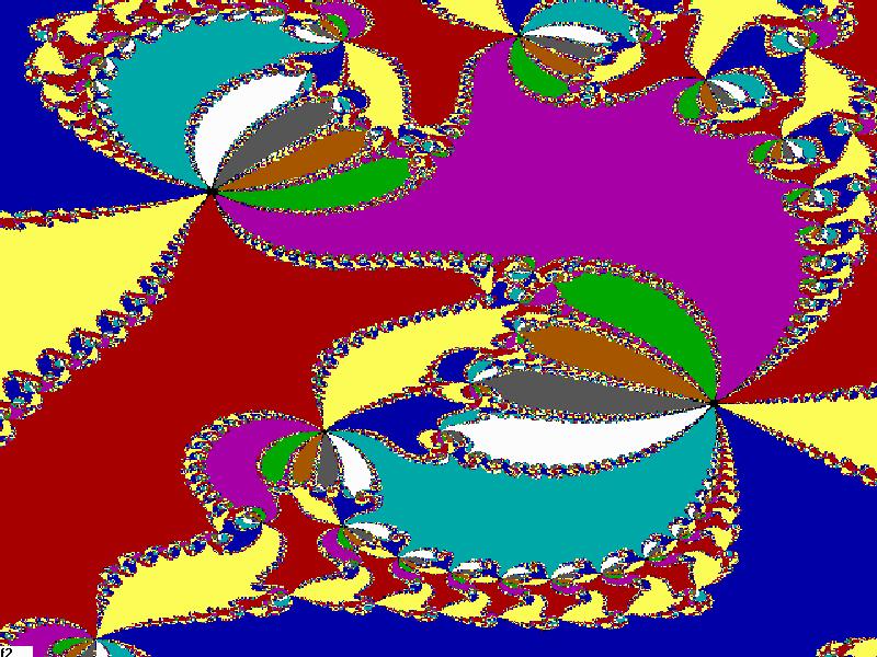
9 4. Examples. a. Z 15-1 =0 For equation Z 15-1=0 we find the following 15 roots with program ROOTNR.BAS or ROOTRF.BAS with a predefined accuracy of.0001 and an allowed number of iteration steps of 50. The accuracy is here defined as an absolute value. The absolute value of the accuracy should be less than a specified small number, here The absolute value of the accuracy is defined as the calculated Z n minus the previously calculated value Z n-1. For small numbers we terminate the iteration process if the relative value of the accuracy is smaller than The roots of this equation (calculated with ROOTNR.BAS and ROOTRF.BAS) are: Root 1: *i Root 2: *i Root 3: *i Root 4: *i Root 5: *i Root 6: *i Root 7: *i Root 8: *i Root 9: *i Root10: *i Root11: *i Root12: *i Root13: D-14*i Root14: *i Root15: *i The pictures of the seed values are shown in the next three pages and were created with program GRAPHNR.BAS, a program that calculates the roots of a complex polynomial function with the Newton-Raphson method. The little white squares in the first two pictures indicate the areas of the next picture. The processes used an accuracy of.0001, and a maximum of 200 iteration steps. No blowout value was defined in this procedure. The defined boundaries of the pictures are respectively defined by the corner values defined by the complex numbers x1+y1.i and x2+y2.i (the frame (window) values) of the rectangular areas used to find the roots. The values x1,y1,x2,y2 are respectively for picture a1:-1,-1,1,1; for picture a2:.6,.4,.8,.6; and for picture a3:.76,.44,.8,.48. A fourth picture a4 shows the seed values and its associated roots when using the Regula Falsi method. The frame (window) values are here the same as in picture a1. The picture was created with program GRAPHRF.BAS, a program that calculates the roots of a complex function with the Regula Falsi method. 9

10 10

11 11

b. Z 9-0.25*Z 6-0.75*Z-1=0 The roots of this equation (calculated with ROOTNR.BAS) are: Root 1: -.5765285440398880+0.8297399226570532*i Root 2: -.8426374259810665-0.2776090046342414*i Root 3: -.

12 b. Z *Z *Z-1=0 The roots of this equation (calculated with ROOTNR.BAS) are: Root 1: *i Root 2: *i Root 3: *i Root 4: *i Root 5: *i Root 6: *i Root 7: D-21*i Root 8: *i Root 9: *i The picture b1 generated with Newton-Raphson is defined through the following properties: frame (window) coordinates:-1,-1,1,1 accuracy:.0001 max. number of iterations: 50 blowout factor: 25 used program: GRAPHNR.BAS 12

c. Z 9 +Z 8 +Z 7 +Z 6 +Z 5 +Z 4 +Z 3 +Z 2 +Z-9=0 The roots of this equation (calculated with ROOTNR.BAS and checked with ROOTFR.BAS) are: Root 1: 0.8767318053938815+0.8813721268235023*i Root 2: 0.

13 c. Z 9 +Z 8 +Z 7 +Z 6 +Z 5 +Z 4 +Z 3 +Z 2 +Z-9=0 The roots of this equation (calculated with ROOTNR.BAS and checked with ROOTFR.BAS) are: Root 1: *i Root 2: *i Root 3: *i Root 4: D-11*i Root 5: *i Root 6: *i Root 7: *i Root 8: *i Root 9: *i The pictures c1 and c2 generated with Newton-Raphson is defined through the following properties: frame coordinates: -1,-1,1,1 (c1) and -.22,.18, -.18,.22 (c2) accuracy:.0001 max. number of iterations: 100 blowout factor: 25 used program: GRAPHNR.BAS Picture c3 is generated with Regula Falsi. frame (window) coordinates: -3,-3,3,3; accuracy: max. number of iterations: 50. program used: GRAPHRF.BAS 13

14 14

d. Z 9 -Z 8 +Z 7 -Z 6 +Z 5 -Z 4 +Z 3 -Z 2 +Z-9=0 The roots of this equation (calculated with ROOTNR.BAS and checked with ROOTRF.BAS) are: Root 1: -.8090169943749472+.5877852522924731*i Root 2:.

15 d. Z 9 -Z 8 +Z 7 -Z 6 +Z 5 -Z 4 +Z 3 -Z 2 +Z-9=0 The roots of this equation (calculated with ROOTNR.BAS and checked with ROOTRF.BAS) are: Root 1: *i Root 2: *i Root 3: *i Root 4: *i Root 5: *i Root 6: D-19*i Root 7: *i Root 8: *i Root 9: *i The picture d1 and d2 generated with program GRAPHNR.BAS (Newton- Raphson) are defined through the following properties: frame coordinates: -1,-1,1,1 (d1) and -.65,-.65,-.55,-.55 (d2) accuracy:.0005 max. number of iterations: 100 Picture d3 was generated with GRAPHRF.BAS (Regula Falsi) and has the following properties: frame (window) coordinates: -1,-1,1,1 accuracy: max. number of iterations:

16 16

e. Z 9 -.95*Z 8 -.9*Z 7 -.85*Z 6 -.8*Z 5 +1.05*Z 4 +1.1*Z 3 +1.2*Z 2 +1.25*Z-1=0 The roots of this equation (calculated with ROOTNR.BAS) are: Root 1: 1.167338901915678-.483216600656D-18*i Root 2:.

17 e. Z *Z 8 -.9*Z *Z 6 -.8*Z *Z *Z *Z *Z-1=0 The roots of this equation (calculated with ROOTNR.BAS) are: Root 1: D-18*i Root 2: D-14*i Root 3: *i Root 4: *i Root 5: *i Root 6: *i Root 7: D-30*i Root 8: *i Root 9: *i The pictures e1 through e4 are generated with GRAPHNR.BAS and are defined through the following properties: frame (window) coordinates: -1,-1,1,1 (e1); -1,.6,-.8,.8 (e2); -.945,.715,-.935,.725 (e3); and ,.7242,-.9369,.7274 (e4) accuracy:.0001 max. number of iterations: 50 Picture e5 was generated with GRAPHRF.BAS and has the following properties: frame (window) coordinates: -1,-1,1,1 accuracy: max. number of iterations: 50 17

18 18

19 19

20 f. C 9 Z 9 +C 8 Z 8 +C 7 Z 7 +C 6 Z 6 +C 5 Z 5 +C 4 Z 4 +C 3 Z 3 +C 2 Z 2 +C 1 Z+C 0 where: C 9 =1 C 8 = i C 7 = i C 6 = i C 5 = i C 4 =1+i C 3 = i C 2 =.8-.5i C 1 =.3-i C 0 =-4+i The roots have been calculated with ROOTNR.BAS and are: Root1: Root2: Root3: Root4: Root5: D-02 Root6: Root7: Root8: Root9: Pictures f1 and f2 are generated with Newton-Raphson and are defined through the following properties: frame (window) coordinates: -1,-1,1,1 (f1) and 0.09,-0.11,.14,-0.05 (f2) accuracy:.0001 max. number of iterations: 50 used program: GRAPHNR.BAS 20

21 21

Fractals, complex equations, and polynomiographs.

Fractals, complex equations, and polynomiographs. Summary: The generation of Mandelbrot and Julia fractals will be revisited in this article. Emphasis will be placed on the way this fractals are created.