Probability, Random Processes and Inference

Transcription

1 INSTITUTO POLITÉCNICO NACIONAL CENTRO DE INVESTIGACION EN COMPUTACION Laboratorio de Ciberseguridad Probability, Random Processes and Inference Dr. Ponciano Jorge Escamilla Ambrosio

2 Course Content 1.3. Discrete Random Variables Basic Concepts Probability Mass Functions Functions of Random Variables Expectation and Variance Joint PMFs of Multiple Random Variables Conditioning Independence 2

3 The Modelling Process A model is an approximate representation of a physical situation. A useful model explains all relevant aspects of a given situation. Mathematical models are used when the observational phenomenon has measurable properties. The model is used to predict the outcome of the experiment, and these predictions are compared with the actual observations that result when the experiment is carried out. 3

4 Computer Simulation Models The predictions of a mathematical model should be treated as hypothetical until the model has been validated through a comparison with experimental measurements. What if the model cannot be validated experimentally because the real system does not exist? Computer simulation models play a useful role in this situation by presenting an alternative means of predicting system behavior, and thus a means of checking the predictions made by a mathematical model. 4

5 Computer Simulation Models A computer simulation model consists of a computer program that simulates or mimics the dynamics of a system. Simulation models are capable of representing systems in greater detail than mathematical models. they tend to be less flexible and usually require more computation time than mathematical models. 5

6 Deterministic Models In deterministic models the conditions under which an experiment is carried out determine the exact outcome of the experiment. In deterministic mathematical models, the solution of a set of mathematical equations specifies the exact outcome of the experiment. Circuit theory is an example of a deterministic mathematical model. Kirchhoff s voltage and current laws, Ohm s law. If an experiment involving the measurement of a set of voltages is repeated a number of times under the same conditions, circuit theory predicts that the observations will always be exactly the same. 6

7 Probability Models Many systems of interest involve phenomena that exhibit unpredictable variation and randomness. We define a random experiment to be an experiment in which the outcome varies in an unpredictable fashion when the experiment is repeated under the same conditions. Deterministic models are not appropriate for random experiments. 7

8 Probability Models Example of a random experiment Suppose a ball is selected from an urn containing three identical balls, labeled 0, 1, and 2. The urn is first shaken to randomize the position of the balls, and a ball is then selected. The number of the ball is noted, and the ball is then returned to the urn. The outcome of this experiment cannot consistently be predicted correctly. 8

9 Random Variables Random variable. Given an experiment with sample space S (the corresponding set of possible outcomes), a random variable (r.v.) is a function from the sample space S to the real numbers R. A random variable X assigns a numerical value X(s) to each possible outcome s of the experiment. The randomness comes from the fact that we have a random experiment (with probabilities described by the probability function P); the mapping itself is deterministic. 9

10 Random Variables A random variable is a real-valued function of the experimental outcome. Real number line R The sample space S is the domain of the random variable, and the set of all values taken on by X is the range of the random variable. 10

11 Random Variables 11

12 Random Variables 12

13 Random Variables Random variables are usually denoted by capital letters from the end of the alphabet, such as X, Y, Z. Related sets are denoted like {s : X(s) = x}, {s : X(s) x}, and {s : X(s) I }, for any number x and any interval I, are events in S. They are usually abbreviated as {X = x}, {X x}, and {X I } and have probabilities associated with them. The assignment of probabilities to all such events, for a given random variable X, is called the probability distribution of X. In the notation for such probabilities, it is usual to write P(X = x), rather than P({X = x}). 13

14 Random Variables Example 1. Three tosses of a coin. Let S = {HHH, HHT, HTH, HTT, THH, THT, TTH, TTT} describe three tosses of a coin, and let X denote the number of heads obtained. Then the values of X, for each outcome s in S, are given in the following table: Thus, in the case of three independent tosses of a fair coin, P(X = 0) = 1/8, P(X = 1) = 3/8, P(X = 2) = 3/8, and P(X = 3) = 1/8. 14

15 Random Variables Example 2. The experiment consists of two rolls of a 4-sided die, and the random variable is the maximum of the two rolls. 15

16 Examples of Random Variables 16

17 Random Variables 17

18 Discrete Random Variables 18

19 Discrete Random Variables (Blitzstein and Hwang, 2015). A random variable X is said to be discrete if there is a finite list of values a 1, a 2,...,a n or an infinite list of values a 1, a 2,... such that P(X = a j for some j) = 1. If X is a discrete r.v., then the finite or countably infinite set of values x such that P(X = x) > 0 is called the support of X. 19

20 Discrete Random Variables Given a random variable, we would like to be able to describe its behavior using the language of probability. For example, we might want to answer questions about the probability that the r.v. will fall into a given range: If M is the number of major earthquakes in Mexico City in the next five years, what is the probability that M equals 0? 20

21 Probability Mass Function The most important way to characterise a random variable is through the probabilities of the values that it can take. For a discrete random variable X, these are captured by the probability mass function (PMF) of X, denoted as p X. 21

22 Probability Mass Function The probability mass function (PMF) of a discrete r.v. X is the function p X given by p X (x) = P(X = x). Note that this is positive if x is in the support of X, and 0 otherwise. In particular, if x is any possible value of X, the probability mass of x, denoted p X (x) is the probability of the event {X = x} consisting of all outcomes that give rise to a value of X equal to x: p X (x) = P(X = x). 22

23 Probability Mass Function In writing P(X = x), we are using X = x to denote an event, consisting of all outcomes s to which X assigns the number x. This event is also written as {X = x}; formally, {X = x} is defined as {s S : X(s) = x}, but writing {X = x} is shorter and more intuitive. 23

24 Probability Mass Function Example 3. (Coin two tosses). Consider an experiment where we toss a fair coin twice. The sample space consists of four possible outcomes: S = {HH, HT, TH, TT}. Let X be the number of Heads. This is a random variable with possible values 0, 1, and 2. Viewed as a function, X assigns the value 2 to the outcome HH, 1 to the outcomes HT and TH, and 0 to the outcome TT. That is, X(HH) = 2, X(HT) = X(TH) = 1, X(TT) = 0. Find the PMFs of the random variable X. 24

25 Probability Mass Function X, the number of Heads. Since X equals 0 if TT occurs, 1 if HT or TH occurs, and 2 if HH occurs, the PMF of X is the function p X given by: p X (0) = P(X = 0) = 1/4, p X (1) = P(X = 1) = 1/2, p X (2) = P(X = 2) = 1/4, 25

26 Probability Mass Function Example 4. Three tosses of a coin. Let X be the number of heads obtained in three independent tosses of a fair coin, as in the previous example. Find the PMF of X. 26

27 Probability Mass Function Example 4. Three tosses of a coin. Let X be the number of heads obtained in three independent tosses of a fair coin, as in the previous example. Find the PMF of X. 27

28 Probability Mass Function Note that in all the previous examples: where in the summation above, x ranges over all the possible numerical values of X. This follows from the additivity and normalisation axioms: as x ranges over all possible values of X, the events {X = x} are disjoint and form a partition of the sample space. 28

29 Probability Mass Function By a similar argument, for any set S X of possible values of X, we have: Then, for x k in S X, we have: 29

30 Probability Mass Function The events A 1, A 2, form a partition of S. These events are disjoint. Let j k, then: since each ζ is mapped into one and only one value in S X. 30

31 Probability Mass Function Next we show that S is the union of the A k s. Every ζ in S is mapped into some x k so that every ζ belongs to an event A k in the partition. Therefore: All events involving the random variable X can be expressed as the union of events A k s. For example, suppose we are interested in the event X in B = {x 2, x 5 }, then: 31

32 Probability Mass Function The PMF p X (x) satisfies three properties that provide all the information required to calculate probabilities for events involving the discrete random variable X: 32

33 Probability Mass Function Property (i) is true because the PMF values are defined as a probability, p X (x) = P[X = x]. Property (ii) follows because the events A k = {X = x k } form a partition of S. Next consider property (iii). Any event B involving X is the union of elementary events, so by Axiom III we have: 33

34 Probability Mass Function The PMF of X gives us the probabilities for all the elementary events from S X. The probability of any subset of S X is obtained from the sum of the corresponding elementary events. In fact we have everything required to specify a probability law for the outcomes in S X. If we are only interested in events concerning X, then we can forget about the underlying random experiment and its associated probability law and just work with S X and the PMF of X. 34

35 Probability Mass Function For example, if X is the number of heads obtained in two independent tosses of a fair coin, then the probability of at least on head is: Recall that: 35

36 Probability Mass Function 36

37 Probability Mass Function For every possible value x, we collect all the outcomes that give rise to X = x and add their probabilities to obtain p X (x). 37

38 Probability Mass Function 38

39 Cumulative Distribution Function The cumulative distribution function (CDF) of a random variable (r.v.) X is a function F X (x) mapping R R and is defined by F X (x) = P{s S : X(s) x}. The argument s is usually omitted for brevity, so F X (x) = P{X x}. The CDF F X (x) is non-decreasing with x and must satisfy: lim x F X (x) = 0 and lim x F X (x) = 1. The cumulative distribution function is often referred to simply as the distribution function. 39

40 Cumulative Distribution Function Example 5. Three tosses of a coin. Given the PMF of X obtained in Example 4, obtain the CDF of X. 40

41 Cumulative Distribution Function The CDF of a discrete r.v. is a staircase function, staying constant between the possible sample values and having a jump of magnitude p X (x i ) at each sample value x i. The PMF and the CDF each specify the other for discrete r.v. s. 41

42 Bernoulli Random Variables A random variable X is called a Bernoulli random variable with parameter p, if it has two possible values, 0 and 1, with P(X = 1) = p and P(X = 0) = 1 p = q, where p is any number from the interval [0, 1]. An experiment whose outcome is a Bernoulli random variable is called a Bernoulli trial process. A Bernoulli r.v. has a Bernoulli distribution referred to as X Bern(p). The symbol is read is distributed as. 42

43 Bernoulli Random Variables This number p in Bern(p) is called the parameter of the distribution; it determines which specific Bernoulli distribution we have. There is not just one Bernoulli distribution, but rather a family of Bernoulli distributions, indexed by p. The indicator random variable of an event A is the r.v. which equals 1 if A occurs and 0 otherwise. We will denote the indicator r.v. of A by I A or I(A). Note that I A Bern(p) with p = P(A). The parameter p is often called the success probability of the Bern(p) distribution. 43

44 Bernoulli Random Variables Example 6. Consider the toss of a coin, which comes up head with probability p, and tail with probability 1 p, The Bernoulli random variable takes the two values 1 and 0, depending on whether the outcome is a head or a tail: Its PMF is: 44

45 Bernoulli Random Variables In practice, for its simplicity the Bernoulli random variable is used to model generic probabilistic situations with just two outcomes, such as: The state of a telephone at a given time that can be either free or busy. A person who can be either healthy or sick with a certain disease. The preference of a person who can be either for or against a certain political candidate. 45

46 Bernoulli trial process A Bernoulli trials process is a sequence of n chance experiments such that: 1. Each experiment has two possible outcomes, which we may call success and failure. 2. The probability p of success on each experiment is the same for each experiment, and this probability is not affected by any knowledge of previous outcomes. The probability q of failure is given by q = 1 p. 46

47 Bernoulli trial process analysis To analyze a Bernoulli trials process, choose as the sample space a binary tree and assign a probability distribution to the paths in this tree. Define X to be the random variable which represents the outcome of the process, i.e., an ordered triple of S s and F s. Let the outcome of the ith trial be denoted by the random variable X i, with distribution function m i. An outcome for the entire experiment will be a path through the tree. For example, 3 represents the outcomes SFS. This suggests assigning probability pqp to the outcome 3. More generally, we assign a distribution function m( ) for paths by defining m( ) to be the product of the branch probabilities along the path. Thus, the probability that the three events S on the first trial, F on the second trial, and S on the third trial occur is the product of the probabilities for the individual events. 47

48 Bernoulli trial process analysis 48

49 Binomial Random Variable Suppose that n independent Bernoulli trials are performed, each with the same success probability p, and failure probability q = 1 p. Let X be the number of successes. Given this, X is called a binomial random variable with parameters n and p. The PMF of X consists of the binomial probabilities calculated as: 49

50 Binomial Random Variable Example 7. Let the probability of n Bernoulli trials having exactly k successes be denotes by b(n, p, k). Let us calculate the particular value b(3, p, 2) from our tree measure. We see that there are three paths which have exactly two successes and one failure, namely 2, 3, and 5. Each of these paths has the same probability p 2 q. Thus b(3, p, 2) = 3 p 2 q. 50

51 Binomial Random Variable Considering all possible numbers of successes we have: 51

52 Binomial Random Variable Carrying out a tree measure for n experiments and determining b(n, p, k) for the general case of n Bernoulli trials, the probability of exactly k successes is: 52

53 Binomial Random Variable Proof. Construct a tree measure as described above. We want to find the sum of the probabilities for all paths which have exactly j successes and n k failures. Each such path is assigned a probability p k q n k. How many such paths are there? To specify a path, we have to pick, from the n possible trials, a subset of k to be successes, with the remaining n k outcomes being failures. We can do this in n k ways. Thus the sum of the probabilities is: with QED 53

54 Binomial Random Variable Example 8. A fair coin is tossed six times. What is the probability that exactly three heads turn up? 54

55 Binomial Random Variable Example 8. A fair coin is tossed six times. What is the probability that exactly three heads turn up? 55

56 Binomial Random Variable Example 9. A die is rolled four times. What is the probability that we obtain exactly one 6? 56

57 Binomial Random Variable Example 9. A die is rolled four times. What is the probability that we obtain exactly one 6? 57

58 Binomial PMF for various values of n and p 58

59 Binomial Distribution Function Let n be a positive integer, and let p be a real number between 0 and 1. Let X be the random variable which counts the number of successes in a Bernoulli trials process with parameters n and p. Then the distribution of X is called the binomial distribution function with parameters n and p. We write X Bin(n, p) to mean that X has the binomial distribution function with parameters n and p. 59

60 Binomial Distribution Function The binomial distribution function of a binomial random variable is given by: 60

61 Geometric Random Variable Suppose that we repeatedly and independently toss a coin with probability of head equal to p, where 0 p 1. The geometric random variable is the number X of tosses needed for a head to come up for the first time. Its PMF is given by: Since (1 p) k 1 p is the probability of the sequence consisting of k 1 successive tails followed by a head. 61

62 Geometric Random Variable This is a legitimate PMF because: Generally, we can interpret the geometric random variable in terms of repeated independent trials until the first success. Each trial has probability of success p and the number of trials until (and including) the first success is modelled by the geometric random variable. 62

63 Geometric Random Variable Example 9. Message transmission. Let X be the number of times a message needs to be transmitted until it arrives correctly at its destination. Find the PMF of X. Find the probability that X is an even number. 63

64 Geometric Random Variable 64

65 Geometric Random Variable The PMF of a geometric random variable decreases as a geometric progression with parameter 1 p. 65

66 Poisson Random Variable A Poisson random variable has a PMF given by: where is a positive parameter characterising the PMF. This is a legitimate PMF because: 66

67 Poisson Random Variable If 1, then the PMF is monotonically decreasing with k, while if 1, then the PMF first increases and then decreases. 67

68 Poisson Random Variable The Poisson PMF with parameter is a good approximation for a binomial PMF with the parameters n and p. i.e.: provided = np, n is very large, and p is very small. 68

69 Poisson Random Variable Example 10. Let n = 100 and p = Calculate the probability of k = 5 successes in n = 100 trials using the binomial PMF. Calculate the Poisson PMF with = np and compare results. 69

70 Poisson Random Variable 70

71 Discrete Uniform Random Variable Discrete Uniform Random Variable. Parameters: a, b, a b Experiment: Pick one of a, a + 1,,b at random; all equally likely Sample space: {a, a + 1,,b} Random variable X: X( ) = Model of: complete ignorance 71

72 Discrete Uniform Random Variable Discrete Uniform Random Variable. Let C be a finite, nonempty set of numbers. Choose one of these numbers uniformly at random (i.e., all values in C are equally likely). Call the chosen number X. Then X is called discrete uniform random variable and have the Discrete Uniform distribution with parameter C; we denote this by X DUnif(C). 72

73 Discrete Uniform Random Variable The PMF of X DUnif(C) is: for x C (and 0 otherwise), since a PMF must sum to 1. As with questions based on the naive definition of probability, questions based on a Discrete Uniform distribution reduce to counting problems. Specifically, for X DUnif(C) and any A C, we have: 73

74 Discrete Uniform Random Variable Example 11. Let s consider the relationship between relative frequencies and the PMF p X (x k ). Suppose we perform n independent repetitions to obtain n observations of the discrete random variable X. Let N k (n) be the number of times the event X = x k occurs and let be f k (n) = N k (n)/n the corresponding relative frequency. As n becomes large we expect that f k (n) p X (x k ). Therefore the graph of relative frequencies should approach the graph of the PMF. 74

75 Discrete Uniform Random Variable Relative frequency and corresponding uniform PMF. 75

76 Functions of Random Variables For an experiment with sample space S, an r.v. X, and a function ɡ : R R, ɡ(X) is the r.v. that maps s to ɡ(X(s)) for all s S. A function of a random variable is a random variable. If X is a random variable, then X 2, e X, and sin(x) are also random variables, as is ɡ(X) for any function ɡ : R R. 76

77 Functions of Random Variables Example 1. Taking ɡ(x) = x, ɡ(x) is the composition of the function X and ɡ First apply X, then apply ɡ 77

78 Functions of Random Variables Given a discrete r.v. X with a known PMF, how can we find the PMF of Y = ɡ(X)? In the case where ɡ is a one-to-one function, the support of Y is the set of all ɡ(x) with x in the support of X, and: P(Y = ɡ(x)) = P(ɡ(X) = ɡ(x)) = P(X = x) 78

79 Functions of Random Variables P(Y = ɡ(x)) = P(ɡ (X) = ɡ(x)) = P(X = x) 79

80 Functions of Random Variables A strategy for finding the PMF of an r.v. with an unfamiliar distribution: try to express the r.v. as a one-to-one function of an r.v. with a known distribution. Example 2. A particle moves n steps on a number line. The particle starts at 0, and at each step it moves 1 unit to the right or to the left, with equal probabilities. Assume all steps are independent. Let Y be the particle s position after n steps. Find the PMF of Y. 80

81 Functions of Random Variables Consider each step to be a Bernoulli trial, where right is considered a success and left is considered a failure. Then the number of steps the particle takes to the right is a Bin(n, 1/2) random variable, which we can name X. If X = j, then the particle has taken j steps to the right and n j steps to the left, giving a final position of j (n j) = 2j n. So we can express Y as a one-to-one function of X, namely, Y = 2X n. Since X takes values in {0, 1, 2,..., n}, Y takes values in { n, 2 n, 4 n,..., n}. 81

82 Functions of Random Variables The PMF of Y can then be found from the PMF of X: P(Y = k) = P(2X n = k) = P(X = (n + k)/2) = n n+k if k is an integer between n and n (inclusive) such that n + k is an even number. If ɡ is not one-to-one, then for a given y, there may be multiple values of x such that ɡ(x) = y. To compute P(ɡ(X) = y), we need to sum up the probabilities of X taking on any of these candidate values of x n 82

83 Functions of Random Variables (PMF of ɡ(X)). Let X be a discrete r.v. and ɡ : R R. Then the support of ɡ(X) is the set of all y such that ɡ(x) = y for at least one x in the support of X, and the PMF of ɡ(X) is: for all y in the support of ɡ(X). 83

84 Functions of Random Variables Example 3. Let Y = X, if the PMF p X (x) is given as: obtain the PMF p Y (y). 84

85 Functions of Random Variables Solution. The possible values of Y are y = 0,1,2, 3, 4. To compute p Y (y) for some given value y from this range, we must add p X (x) over all values x such that x = y. 85

86 Functions of Random Variables Solution 86

87 Expectation and Variance Given a list of numbers x 1, x 2,..., x n Their arithmetic mean is defined by Generalizing, we can define a weighted mean of x 1, x 2,..., x n as: where the weights p 1,...,p n are pre-specified nonnegative numbers that add up to 1. 87

88 Expectation and Variance The expected value (also called the expectation or mean) of a discrete r.v. X whose distinct possible values are x 1, x 2,... is defined by: If the support is finite where the sum is over the support of X. 88

89 Expectation and Variance The expected value of X is a weighted average of the values that X can take on, weighted by the probability mass of each value. E(X) depends only on the distribution of X. The mean can be seen as a representative value of X, which lies somewhere in the middle of its range. From here, the mean can be seen as the centre of gravity of the PMF. 89

90 Expectation and Variance If the PMF is symmetric around a certain point, that point must be equal to the mean. 90

91 Elementary Properties of Expectation If X 0, then E[X] 0 If a X b, then a E[X] b If c is a constant, then E[c] = c 91

92 Expectation and Variance Example 1. Let X be the number of heads in three tosses of a fair coin. Find E[X]. 92

93 Expectation and Variance Example 1. Let X be the number of heads in three tosses of a fair coin. Find E[X]. 93

94 Expectation and Variance Example 2. Consider two independent coin tosses, each with a ¾ probability of a head, and let X be the number of heads obtained. This is a binomial r.v. with parameters n = 2 and p = ¾. Its PMF is: So the mean is: 94

95 Expectation and Variance Example 2. Consider two independent coin tosses, each with a ¾ probability of a head, and let X be the number of heads obtained. This is a binomial r.v. with parameters n = 2 and p = ¾. Its PMF is: So the mean is: 95

96 Moments and Variance The nth moment of a discrete random variable X is defined as: The expected value of the variable X n. The most common moments used are the first and second moments. The first moment is what we previously referred to as the mean. 96

97 Moments and Variance The second moment of the random variable X is the expected value of the random variable X 2. 97

98 Moments and Variance The central moment of the discrete random variable X is defined as: where μ X = E[X] is the mean (first moment) of the random variable. The central moment of a random variable is the moment of that random variable after its expected value is subtracted. 98

99 Moments and Variance The first central moment is always zero. The second central moment of a discrete random variable is its variance: with μ X = E[X]. The variance is always nonnegative. The variance provides a measure of dispersion of X around its mean. 99

100 Moments and Variance Note that: In many cases the best way to calculate the variance of a r.v. is to calculate the first two moments and then form the second moment minus the first moment squared. 100

101 Standard Deviation The standard deviation is defined as the squared root of the variance: Both the variance and the standard deviation serve as a measure of the width of the PDF of a random variable. 101

102 Expected Value Rule for Functions of Random Variables Given the discrete random variable X with PMF p X, the expected value of a function, g(x), of that random variable is given by: Using this rule, the variance of X can be obtained as: 102

103 Variance Example 1. Consider the random variable X, which has PMF p X (x) given as: The mean E[X] is equal to 0, which can be verified by: 103

104 Variance Let Z= (X E[X]) 2 = X 2. Then we have: The variance of X is then obtained by: 104

105 Variance Calculate the variance using the Expected value rule. Let Y = g(x) and use the formula: Then we have: 105

106 Variance Using the expected value rule, the variance of X can be calculated as: For the random variable of the example we have: 106

107 Variance Example 2. Roll of a Die. Let X denote the number obtained in a roll of a die. Obtain the mean an variance of X. 107

108 Variance Example 2. Roll of a Die. Let X denote the number obtained in a roll of a die. Obtain the mean an variance of X. P(X = i) = 1/6 for i = 1, 2,..., 6. Then μ = 3.5, and 108

109 Variance 109

110 Standardization In some applications, we transform random variables to a standard scale in which all random variables are centred at 0 and have standard deviations equal to 1. For any given r.v. X, for which μ and σ exist, we define its standardization as the new r.v. 110

111 Mean and Variance of a Linear Function Let X be a random variable and let : Y = ax + b Where a and b are given scalars. Then: 111

112 Mean and Variance of a Linear Function 112

113 Mean and Variance of Common r.v. Bernoulli 113

114 Mean and Variance of Common r.v. Poisson 114

115 Mean and Variance of Common r.v. Discrete uniform r.v. where a and b are two integers with a b. Then the mean is: 115

116 Joint PMFS of Multiple Random Variables We usually deal with the relationship between multiple r.v.s in the same experiment. Medicine: To evaluate the effectiveness of a treatment, we may take multiple measurements per patient; an ensemble of blood pressure, heart rate, and cholesterol readings can be more informative than any of these measurements considered separately. Time series: To study how something evolves over time, we can often make a series of measurements over time, and then study the series jointly. There are many applications of such series, such as global temperatures, stock prices, or national unemployment rates. The series of measurements considered jointly can help us deduce trends for the purpose of forecasting future measurements. 116

117 Joint PMFS of Multiple Random Variables Consider two discrete random variables X and Y associated with the same experiment. The probabilities of the values that X and Y can take are captured by joint PMF of X and Y, denoted p X,Y. If (x,y) is a pair of possible values of X and Y, the joint PMF of X and Y is the function p X,Y given by: The joint PMF of n r.v.s is defined analogously. 117

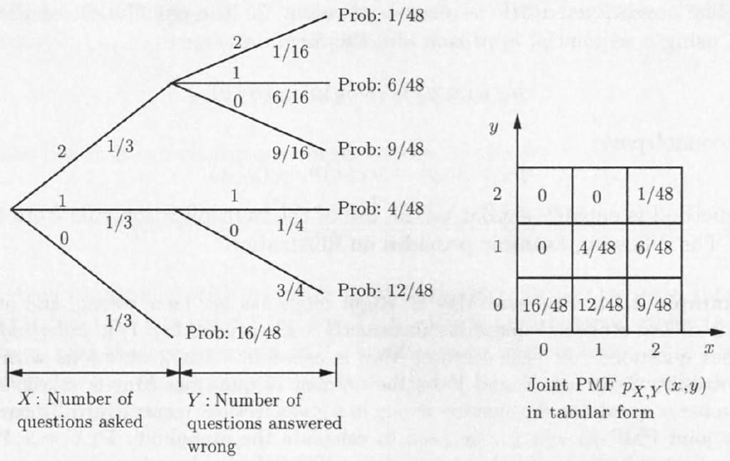
118 Joint PMFS of Multiple Random Variables 118

119 Joint PMFS of Multiple Random Variables Just as univariate PMFs must be nonnegative and sum to 1, joint PMFs must be nonnegative and sum to 1, where the sum is taken over all possible values of X and Y : The joint PMF determines the probability of any event that can be specified in terms of the r.v.s X and Y. 119

120 Joint PMFS of Multiple Random Variables In terms of their joint sample space: 120

121 Joint PMFS of Multiple Random Variables The joint PMF determines the probability of any event that can be specified in terms of the r.v.s X and Y. For example if A is the set of all pairs (x,y) that have certain property, then: 121

122 Joint PMFS of Multiple Random Variables From the joint distribution of X and Y, the PMF of X alone can be obtained by summing over the possible values of Y. The same apply for the case of obtaining the PMF of Y: 122

123 Joint PMFS of Multiple Random Variables In the context of joint distributions, we will call it the marginal or unconditional distribution of X, to make it clear that we are referring to the distribution of X alone, without regard for the value of Y. For discrete r.v.s X and Y, the marginal PMF of X is: 123

124 Joint PMFS of Multiple Random Variables The operation of summing over the possible values of Y in order to convert the joint PMF into the marginal PMF of X is known as marginalizing out Y.. The marginal PMF of X is the PMF of X, viewing X individually rather than jointly with Y. 124

125 Joint PMFS of Multiple Random Variables Example 1. Maximum and Minimum of Three Integers. Choose three numbers X 1, X 2, X 3 without replacement and with equal probabilities from the set {1, 2, 3, 4}, and let X = max{x 1, X 2, X 3 } and Y = min{x 1, X 2, X 3 }. Find the joint PMF of X and Y. 125

126 Joint PMFS of Multiple Random Variables Solution. Table 1 lists the set of all 24 possible outcomes, together with the values of X and Y : 126

127 Joint PMFS of Multiple Random Variables Now, each possible outcome has probability 1/24, and so we just have to count the number of times each pair of X, Y values occurs and multiply it by 1/24 to get the PMF p X,Y. This PMF is given in Table 2, together with the marginal probabilities p Y (y) on the right and p X (x) at the bottom. 127

128 Joint PMFS of Multiple Random Variables The joint PMF and marginals of X = max(x 1, X 2, X 3 ) and Y = min(x 1, X 2, X 3 ) 128

129 Functions of Multiple Random Variables A function Z = ɡ(X,Y) of the random variables X and Y defines another random variable. Its PMF can be calculated from the joint PMF p X,Y according to: 129

130 Functions of Multiple Random Variables The expected value rule applies and takes the form: In the case where ɡ is linear and of the form ax+by+c, where a, b, c are given scalars: 130

131 More than Two Random Variables The joint PMF of three random variables X, Y and Z is defined as: for all the possible triplets of numeric values (x,y,z). The corresponding marginal are obtained as: 131

132 More than Two Random Variables The expected value rule for functions is given by: If ɡ is linear and has the form ax+by+cz+d, then: 132

133 Conditioning Conditional PMF. The PMF of a random variable X, conditioned on a particular event A with P(A) 0, is defined by: As the events {X = 0} A are disjoint for different values of x, their union is A, therefore: 133

134 Conditioning Combining the previous two formulas: so p X A is a legitimate PMF. The conditional PMF is calculated similar to its unconditional counterpart: to obtain p X A we add the probabilities of the outcomes that give rise to X = x and belong to the conditioning event A, and then normalise by dividing with P(A). 134

135 Conditioning 135

136 Conditioning Example 1. Let X be the roll of a fair six-sided die and let A be the event that the roll is an even number, obtain p X A. By applying the preceding formula, we obtain: 136

137 Conditioning one Random Variable on Another Let X and Y be two r.v.s associated with the same experiment. The conditional PMF p X Y of X given Y = y is: Using the definition of conditional probabilities: 137

138 Conditioning one Random Variable on Another 138

139 Conditioning The conditional PMF is often convenient for the calculation of the joint PMF, using a sequential approach and the formula: Or its counterpart: 139

140 Conditioning 140

141 Conditioning 141

142 Conditioning 142

143 Conditioning The conditional PMF can also be used to calculate the marginal PMFs: In essence this calculation is identical to the total probability theorem but casted in different notation. 143

144 Conditioning Example 3. Consider a transmitter that is sending messages over a computer network. Let us define the following two random variables: X: the travel time of a given message, Y: the length of the given message Knowing the PMF of the travel time of a message that has a given length, and the PMF of the message length, find the (unconditional) PMF of the travel of a message. 144

145 Conditioning Solution. Assuming that the length of the message can take two possible values: y =10 2 bytes with probability 5/6 y = 10 4 bytes with probability 1/6 Assume that the travel time X of the message depends on its length Y and the congestion in the network at the time of transmission. 145

146 Conditioning In particular, the travel time is 10-4 Y seconds with probability 1/2, 10-3 Y seconds with probability 1/3, and 10-2 Y seconds with probability 1/6. Thus: 146

147 Conditioning To find the PMF of X, use the total probability formula: Therefore: 147

148 Conditioning 148

149 Conditioning 149

150 Conditioning 150

151 Conditional Expectation A conditional expectation is the same as an ordinary expectation, except that it refers to the new universe. All probabilities and PMFs are replaced by their conditional counterparts. Conditional variance can also be treated similarly. 151

152 Conditional Expectation 152

153 Conditional Expectation 153

154 Conditional Expectation 154

155 Conditional Expectation 155

156 Conditional Expectation Example 4. Messages transmitted by a computer in Boston through a data network are destined for New York with probability 0.5, for Chicago with probability 0.3, and for San Francisco with probability 0.2. The transit time X of a message is random. Its mean is 0.05 seconds if it is destined for New York, 0.1 seconds if it is destined for Chicago, and 0.3 seconds if it is destined for San Francisco. Then, E[X] is easily calculated using the total expectation theorem as 156

157 Independence of a Random Variable from an Event The independence of a random variable from an event is similar to the independence of two events. Knowing the occurrence of the conditioning event provides no new information on the value of the random variable. Formally, the random variable X is independent of the event A if: so that as long as P(A) 0, independence is the same as the conditioning: 157

158 Independence 158

159 Independence 159

160 Independence of Random Variables Two random variables X and Y are independent if: This is the same as requiring that the two events {X = x} and {Y = y} be independent for every x and y. The formula shows that independence is equivalent to the condition: This means that the value of Y provides no information on the value of X. 160

161 Independence of Random Variables There is a similar notion of conditional independence of two random variables, given an even A wit P(A) > 0. Let X and Y said to be conditional independent, given a positive probability event A, if: 161

162 Independence of Random Variables 162

163 Independence of Random Variables In a similar calculation it can be shown that if X and Y are independent, then: for any functions ɡ and h. This follows immediately once we realise that if X and Y are independent, then the same is true for ɡ(x) and h(y). 163

164 Independence of Random Variables Consider now the sum X + Y of two independent random variables and let calculate its variance. Considering zero-mean random variables and, then we have: The variance of the sum of two independent random variables is equal to the sum of their variances 164

165 Independence of Random Variables 165

166 Independence of Random Variables 166

167 Independence of Several Random Variables Three random variables X, Y, and Z are said to be independent if: If X, Y, and Z are independent random variables, then any three random variables f(x), g(y), and h(z), are also independent. The random variables of the form g(x,y) and h(y,z) are usually not independent because they are both affected by Y. 167

168 Variance of the Sum of Independent Random Variables If X 1, X 2,,X n are independent random variables, then: 168

169 Variance of the Sum of Independent Random Variables 169

170 Variance of the Sum of Independent Random Variables 170

171 Variance of the Sum of Independent Random Variables The formulas for the mean and variance of a weighted sum of random variables form the basis for many statistical procedures that estimate the mean of a random variable by averaging many independent samples. 171

172 Mean and Variance of the Sample Mean 172

173 Mean and Variance of the Sample Mean 173

174 Mean and Variance of the Sample Mean 174

175 Summary of Results for Special Random Variables 175

176 Summary of Results for Special Random Variables 176

177 Summary of Results for Special Random Variables 177