More on Adaptive Learning and Applications in Monetary Policy. Noah Williams

Transcription

1 More on Adaptive Learning and Applications in Monetary Policy Noah University of Wisconsin - Madison Econ 899

2 Beyond E-Stability: Perpetual Learning Orphanides and J. (2005). Lucas-type aggregate supply curve for inflation π t : π t+1 = φπ e t+1 + (1 φ)π t + αy t+1 + e t+1, Output gap y t+1 is set by monetary policy up to white noise control error y t+1 = x t + u t+1. Policy objective function L = (1 ω)var(y) + ωvar(π π ) gives rule x t = θ(π t π ). where under RE θ = θ P (ω, φ, α).

3 Perpetual Learning Under RE inflation satisfies π t = c 0 + c 1 π t 1 + v t. Under learning private agents estimate coefficients by constant gain (or discounted) least squares. Older data dated discounted at rate (1 ε). Discounting of data natural if agents are concerned to track structural shifts. There is empirical support for constant gain learning. With constant gain, LS estimates fluctuate randomly around ( c 0, c 1 ): there is perpetual learning and π e t+1 = c 0,t + c 1,t π t.

4 Perpetual Learning Results Perpetual learning increases inflation persistence. Naive application of RE policy leads to inefficient policy. Incorporating learning into policy response can lead to major improvement. Efficient policy is more hawkish, i.e. under learning policy should increase θ to reduce persistence. This helps guide expectations. Following a sequence of unanticipated inflation shocks, inflation doves (i.e. policy-makers with low θ) can do very poorly, as expectations become detached from RE. If agents know π and only estimate the AR(1) parameter the policy trade-off is more favorable.

5 Learning and inflation persistence Preceding analysis was an example of empirics based on calibration. Now we consider work that estimates learning dynamics (Milani 2005, 2007). The source of inflation persistence is subject to dispute. For good empirical fit, a backward-looking component is needed in the NK Phillips curve. The bulk of the literature assumes RE, but learning could be a reason for inflation persistence. Incorporate indexation to Calvo price setting: non-optimized prices indexed to past inflation. This yields π t γπ t 1 = δx t + βe t (π t+1 γπ t ) + u t, where x t is the output gap. Earlier work under RE finds γ 1.

6 Inflation under learning The preceding can be written as π t = γ 1 + βγ π t 1 + β 1 + βγ E t π t+1 + δ 1 + βγ x t + u t. For expectations assume a PLM π t = φ 0,t + φ 1,t π t 1 + ε t Agents use data {1, π i } t 1 0 to estimate φ 0, φ 1 using constant gain LS. The implied ALM is π t = βφ 0,t(1 + φ 1,t ) 1 + βγ + γ + βφ2 1,t 1 + βγ π t 1 + δ 1 + βγ x t + u t. Alternatively, could use with real marginal cost as the driving variable.

7 Empirical Model Data: GDP deflator, output gap is detrended GDP, real marginal cost is proxied by deviation of labor income share from 1960:01 to 2003:04. Initialization: agents initial parameter estimates obtained by using pre-sample data Methodology: PLM estimated from constant-gain learning using ε = Then estimate ALM using nonlinear LS, which separates learning effects from structural effects. Note: Simultaneous estimation of learning rule and the model would be much more ambitious.

8 Empirical Results PLM parameters: (i) φ 1,t initially low in 1950s and 60s, then higher (up to 0.958), then some decline to values above 0.8. (ii) φ 0,t initially low, then became much higher and then gradual decline after ALM structural estimates: Degree of indexation γ = (with output gap & ε = 0.015) and declining for higher ε. Model fit criterion (Schwartz BIC) suggest values ε (0.015, 0.03), with best fit at ε = Conclusion: Estimates for γ not significantly different from zero. Results are very different from those obtained under RE, which finds γ 1. Milani has also estimated full NK models under learning. He finds that also the degree of habit persistence is low in IS curve.

9 Learning by Policymakers So far have focused on learning by private agents and its implications for policy. However policymakers as well must learn about the economy. Beliefs of policymakers very influential, since they are large agents. Variation in beliefs or misspecification of model by policymakers can have a large impact on equilibrium dynamics. Sargent (1999) showed that misspecification and learning by policymakers can lead to temporary improvements in outcomes: Escaping Nash Inflation Model analyzed by Cho,, and Sargent (2002), Sargent and (2005), estimated by Sargent,, and Zha (2006)

10 The Conquest Model The economy is a simple rational expectations natural rate Phillips curve model: U n = u (π n ˆx n ) + σ 1 W 1n π n = x n + σ 2 W 2n ˆx n = x n Rational expectations: - Time consistency problem. - Nash inflation (u) > Ramsey inflation (0). Here: - Public has rational expectations. - Government doesn t know Phillips curve, learns adaptively.

11 The Government s Beliefs Government s Phillips curve model: Beliefs: γ = [γ 1, γ 1 ]. U n = γ 1 π n + γ 1 + η n, Can generalize to allow lags of inflation, unemployment in regression. Govt. treats regression error as orthogonal: ( [ ]) πn Ê η n = 0. 1 Use notation: Êg(γ, ξ n ) = 0.

12 The Government s Problem Based on estimates, each period government solves: ( ) min Ê U 2 x n + πn 2 n Results in feedback policy: x n = h(γ). A self-confirming equilibrium (SCE) is a vector γ such that the government s beliefs are confirmed by its observations: Eg(γ, ξ n ) = 0, where : - (U n, π n ) follow the true evolution given x n - x n solves government s problem given γ. Note: Unique SCE with Nash inflation level. If γ 1 = 0, x n = 0 : Ramsey outcome.

13 Adaptation of Beliefs Government updates beliefs γ n based on data. Sets inflation as h(γ n ). Govt. believes data are generated by: U n = α n 1Φ n + η n, (Eη 2 n = σ 2 ) α n = α n 1 + Λ n, (cov(λ n ) = V ) where Φ n = [π n, 1]. Update beliefs using CG RLS: γ n+1 = γ n + ɛrn 1 g(γ n, ξ n ) R n+1 = R n + ɛ(φ n Φ n R n ), Implicitly assumes V = ɛ 2 σ 2 E(ΦΦ ) 1 and σ = σ 1 (regression error=unemployment shocks) In this case, Kalman filter and RLS have same limits, different transient behavior. Sargent and (2005) study more general priors on V.

14 Learning in the Model Stability of SCE governed by same E-stability results as before. Find that SCE is E-stable, suggests beliefs should converge to it. However in simulations observe repeated episodes of decreases in inflation from Nash level down to Ramsey/commitment level of zero. The low inflation episodes are driven by reductions in government s estimated Phillips curve slope to near zero. Analyze the escape dynamics characterizing movements away from the SCE.

15 Conquest of American Inflation

16 Escape Dynamics Escape = beliefs fixed distance from SCE Convergence theorem probability of escape 0 as ε 0. For fixed ε, may be rare escapes. If an unlikely event occurs, it is very likely to occur in the most likely way. ( ), CWS determine: - most likely escape direction and full time path - probability of escape and bounds on escape times

17 Characterzing Escapes To find most likely escape path, find least cost perturbations v that push the beliefs out of a set G containing the SCE. Solve the least-squares control problem: s.t. 1 T S = inf { v,t} 2 0 γ = R 1 g(γ) + v γ(0) = γ, γ(t) / G. v(s) Q(γ(s)) 1 v(s)ds Minimizing path is most likely as w.p.1 all escape paths become close to minimizing path as ε 0. Times between escapes increase exponentially as ε 0, minimized value S determines rate of increase.

18 Distribution of Escapes

19 Direction of Escapes

20 Escape Paths

21 Interpretation of Results Starting at SCE, central bank downweights past observations. Occasionally will get a sequence of correlated shocks to inflation and unemployment. Implies unemployment varies less for a given inflation rate. Government reads this as a shift in Phillips curve toward more vertical. In response will cut inflation. Since have been near SCE, movements in intended inflation rate very influential for belief estimates. Leads to (locally) self-reinforcing dynamics: government believes Phillips curve even more vertical, cuts inflation more.

22 Implications of Results Once Phillips curve slope is zero, inflation set to zero. Economy remains near there for a while. Eventually shocks to inflation and unemployment make government pick up on true Phillips curve slope. Increases inflation, revises beliefs. But this process is slow. Government can temporarily learn to set optimal policy even if model is misspecified. Suggests lower inflation in US since 1970s may not be driven by changes in Fed s model, but just changes in estimates of that model. Does this story fit empirically?

23 Sargent,, Zha (2006) How to explain the Great Inflation of the 1970s, the decline in 1980s and relative stability in 1990s to the present? Has policy changed? Was it luck (shocks)? Is the improvement in outcomes sustainable? Can policy be modeled in a optimizing manner, rationalizing and explaining rise and fall in US inflation?

24 What We Do Develop structural model of learning with optimizing government. Able to explain rise & fall of inflation. Estimate and analyze predictions. Analyze intermediate and long run behavior of model. Interpretation of US experience: - Policy objective unchanged, but beliefs change over time. As in Sargent (1999), Primiceri (2003a) but different mechanism - Large shocks in 1970s accommodated, led to large inflation. - Not shocks vs. policy, but shocks policy s disinflation due to different govt. beliefs: Believed less or no Phillips curve tradeoff

25 A More General Model Economy: Expectational Phillips curve, govt. controls inflation u t u = θ 0 (π t E t 1 π t ) + θ 1 (π t 1 E t 2 π t 1 ) +τ 1 (u t 1 u ) + σ 1 w 1t, [w 1t N (0, 1)] π t = x t 1 + σ 2 w 2t, [w 2t N (0, 1)] Government problem: minê x t 1 β t ((π t π ) 2 + λ(u t u ) 2 ) t=1 subject to inflation equation and subjective model: u t = ˆα t t 1 Φ t + σw t, Φ t = [π t, π t 1, u t 1, π t 2, u t 2, 1] π t = f (ˆα t t 1 )Φ t

26 Government s Model Govt doesn t account for expectations misspecified model. Key identifying assumption: E [ Φ t (u t Φ tα) ] = 0 Govt always assumes it holds. Actually holds in a self-confirming equilibrium. Govt bases estimates ˆα t t 1 = E t 1 (α) on: u t = α tφ t + σw t, w t N (0, 1) α t = α t 1 + Λ t, Λ t N (0, V ) Updates ˆα t t 1 (and P t t 1 ) via Kalman filter

27 Estimation Estimate govt prior beliefs σ 2 and V along with structure. Fix β =.9936, λ = 1, π = 2, u = 1. Fix ˆα 1 0 on pre-sample regression from Estimate remaining: u, τ 1, θ 0, θ 1, ζ 1 = σ 2 1, ζ 2 = σ 2 2, and C P, C V s.t. C P C P = P 1 0, C V C V = V. Need to normalize σ 2 : would scale with beliefs P t t 1 and V. Set σ = σ 1 : Govt. prior var of u t shocks = true var. Use Bayesian methods (MLE similar). Gaussian likelihood L(I T φ), specify prior p(φ), maximize posterior: p(φ I T ) L (I T φ) p(φ)

28 Inference: Inflation Actual Lower band Higher band From March 1960 to December 2003 Actual vs one-step forecast with 90% error bands

29 Medium Run Dynamics So far have focused on fit one step ahead. Now look out to horizon of 4+ years. Take estimated initial conditions at each date, run 5000 Monte Carlo simulations going forward 50 periods. Focus on 1970s high inflation episodes and early 1980s disinflation. Assess model s implications for rise & fall.

30 Initial Condition: January, Actual Median forecast 10 Inflation rate (percent) Forecast months after 74:01

31 Initial Condition: April, Actual Median forecast 10 Inflation rate (percent) Forecast months after 80:04

32 Interpretation (Our) Previous research in this line has emphasized the time-consistency problem. [In contrast to Blinder (1998).] Not a major issue here: estimate small responses to inflation surprises. Nash inflation close to Ramsey (2.25 % vs. 2%). Government beliefs are still important, but so are shocks. Throughout early 1970s govt believed in Phillips curve tradeoff. One diagnostic: sum of coefficients on inflation. Implied very high perceived sacrifice ratio: very costly in unemployment terms to bring inflation down in response to a shock. Large shocks in 1970s were accommodated.

33 Government Beliefs 1 Sum of π coefs From March 1960 to December 2003 Sum of coefficients on π. If 0 no LR tradeoff.

34 Government s Perceived Sacrifice Ratio Perceived LR u u from switching to 2% inflation

35 Comparison to Literature Primiceri (2006): Different learning with same basic aim. - His fit is more comparable to a VAR. - Emphasizes high perceived sacrifice ratio, but also mismeasurement of natural rate. - Key difference theoretical: his main model is Keynesian, backward-looking. Cogley-Sargent (2006): Government has three different models, adapts weight it puts on them over time. Weight on Samuelson-Solow model low by mid-70s but very high losses if cut inflation, dominates.

36 South American Inflation: Sargent,, Zha (2009) In last 30 years several Latin American countries experienced repeated hyperinflations of % per month. What led to these, and how could they re-occur? Conventional view: Hyperinflation is a fiscal problem. But weak direct empirical results. Unorthodox view: Fiscal/monetary aspects not important. Our approach: Adaptive learning by private sector, time varying seignorage needs, time varying volatility. Minor departure from rational expectations allows us to fit data, provides insights on causes and consequences of hyperinflations. Rehabilitation of fiscal causes.

37 Adaptive and REE dynamics Mean adaptive dynamics and REE dynamics. π t β t G(β t ) π 1 π 2 β t H(β t )

38 Adaptive and REE dynamics Mean adaptive dynamics and REE dynamics. π t β t G(β t ) π 1 π 2 β t H(β t )

39 Adaptive dynamics and escapes Adaptive dynamics and the escape event. π t β t G(β t ) π 1 π 2 β t

40 Adaptive dynamics and escapes Adaptive dynamics and the escape event. π t β t G(β t ) π 1 π 2 β t

41 The Model Money demand: M t P t = 1 γ λ γ Government budget constraint: P e t+1 P t M t = θm t 1 + d t (s t )P t Deficit process, with regimes s t = [m t, v t ] (fiscal policy): d t (m t, v t ) = d(m t ) + η d t (v t ) Pr(m t+1 = i m t = j) = qij m, i, j = 1,..., m h Pr(v t+1 = i v t = j) = qij, v i, j = 1,..., v h {γ,d t (s t )} not identified, so normalize γ = 1 in estimation.

42 Beliefs Private sector forecasts inflation in setting money demand. Assume learns adaptively from past inflation observations. πt+1 b = β t β t = β t 1 + ε(π t 1 β t 1 ) ε is called the gain, giving weight on past observations. We assume it s constant: agents discount past data.

43 No-Breakdown Conditions Equilibrium inflation: π t = θ(1 λβ t 1) 1 λβ t d t (s t ) Makes sense only if numerator and denominator are both positive: Positive prices and positive real balances. For moments of inflation to exist, need denominator bounded away from zero. Thus we require, for some δ > 0: 1 λβ t 1 > 0, 1 λβ t d t (s t ) > δθ(1 λβ t 1 ), Leads to truncated normal distribution for η d.

44 Reforms Possible that a sequence of seignorage shocks pushes beliefs β t above high SS π2. Escape from domain of attraction of lower, stable equilibrium. Makes model unstable. May eventually threaten the no-breakdown conditions. Our solution: Reset inflation (to lower REE plus noise) after threatened breakdowns: π t = π t (s t ) π 1(s t ) + η π t (s t ) where η π is truncated normal. Stands in for cosmetic reforms (exchange rates, capital controls) which did not alter seignorage process. Beliefs may be slow to adjust reforms not immediately credible.

45 Estimation Our parameter estimates maximize the likelihood of a history of inflation, π t, t = 1,..., T. We use the model s joint density and the inflation data to estimate money creation rates and compare to data. The likelihood function is challenging numerically. Blocking and parallel computing come to our rescue.

46 Argentina Conditional SCEs Log Belief log β t βt 0.3 Deficits Data Model Probability 0.8 L deficit Escape log π t Actual Prediction

47 Argentina: Beliefs

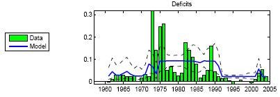
48 Argentina: Deficits

49 Argentina: Escapes and Regimes

50 Argentina: Inflation

51 Argentina Conditional SCEs Log Belief log β t βt 0.3 Deficits Data Model Probability 0.8 L deficit Escape log π t Actual Prediction

52 Brazil 0.5 Conditional SCEs 0.5 Log Belief log β t βt Data Model Deficits Probability 0.8 L & M deficit Escape log π t 0.6 Actual Prediction

53 The Rise and Fall of Hyperinflation Different hyperinflations were driven by different factors (escapes, shocks) and ended by different factors (monetary reform, fiscal deficit reform, smaller shocks). Table: Causes of the rise and fall of hyperinflation across countries Escape No Escape Monetary Reform Brazil (87-91) Peru (87-92) Fiscal Deficit Reform Argentina (87-91) Bolivia (82-86) Brazil (92-95) No Reform (Driven by Chile (71-78) Argentina (76-86) Deficit Shocks)

54 Conclusion Expectations play a large role in modern macroeconomics. People are smart, but boundedly rational. Cognitive consistency principle: economic agents should be about as smart as (good) economists, e.g. model agents as econometricians. Stability of RE under private agent learning is not automatic. Monetary policy must be designed to ensure both determinacy and stability under learning. Policymakers may need to use policy to guide expectations. Under learning there is the possibility of persistent deviations from RE. Appropriate policy design can minimize these risks. Learning dynamics can also help explain persistence of inflation and output dynamics, volatility of inflation, and rises and falls of inflation.