Lecture II. Mathematical preliminaries

Transcription

1 Lecture II Ivica Kopriva Ruđer Bošković Institute 1/58

2 Course outline Motivation with illustration of applications (lecture I) with principal component analysis (PCA)? (lecture II) Independent component analysis (ICA) for linear static problems: information-theoretic approaches (lecture III) ICA for linear static problems: algebraic approaches (lecture IV) ICA for linear static problems with noise (lecture V) Dependent component analysis (DCA) (lecture VI) 2/58

3 Course outline Underdetermined blind source separation (BSS) and sparse component analysis (SCA) (lecture VII/VIII) Nonnegative matrix factorization (NMF) for determined and underdetermined BSS problems (lecture VIII/IX) BSS from linear convolutive (dynamic) mixtures (lecture X/XI) Nonlinear BSS (lecture XI/XII) Tensor factorization (TF): BSS of multidimensional sources and feature extraction (lecture XIII/XIV) 3/58

4 Expectations, moments, cumulants, kurtosis Gradient and optimization: vector gradient, Jacobian, matrix gradient natural and relative gradient, gradient descent, stochastic gradient descent (batch and online) Estimation theory Information theory: entropy, differential entropy, entropy of a transformation, mutual information, distributions with maximum entropy, negentropy, entropy approximation: Gram-Charlier expansion PCA and whitening (batch and online) 4/58

5 The r th order moment of the scalar stochastic process z is defined as r r 1 T r M r ( z) = E z = z f ( zdz ) z( t) t= 1 T where f(z) is pdf of random variable z and T represents sample size. For real stochastic processes z 1 and z 2 the cross-moment is defined as 1 M rp ( z, z ) E z z z ( t) z ( t) r p T r p 1 2 = 1 2 t= T Cross-moment can be defined for nonzero time shifts as i, j, k, l,.. M τ1 τ2 τr 1 = E zi t zj t+ τ1 zk t+ τ2 zl t+ τr 1 rz, (,,..., ) ( ) ( ) ( )... ( ) 1 T z ( ) ( 1 i t zj t+ τ1) zk( t+ τ2)... zl( t+ τr 1) t= T 5/58

6 The first characteristic function of the random process z is defined as jωz jωz Ψ z ( ω) = E e = e f ( zdz ) Power series expansion of ψ z (ω) is obtained as 2 n ( jω) 2 ( jω) n Ψ z ( ω) = E 1 + jωz+ z z ! n! ω ω = + [ ] ! n! 2 n 2 ( j ) n ( j ) 1 E z jω E z... E z... Moments of the random process z are defined as n n 1 d Ψ z( ω) E z = atω 0. n = n j dω 6/58

7 The second characteristic function of the random process z is defined as K ( ω) = ln Ψ ( ω) z Power series expansion of K z (ω) is obtained as z 2 n ( jω) ( jω) n Kz( ω) = C1( z)( jω) + C2( z) C ( z) ! n! where C 1,C 2,.., C n are cumulants of the appropriate order and are defined as C n 1 d Kz ( ω) ( z) = atω = 0. j dω n n n 7/58

8 In practice cumulants, as well as moments, must be estimated from data. For that purpose relations between cumulants and moments are important. It follows from the definition of the first and second characteristic function { K ω } exp ( ) =Ψ ( ω) After Taylor series expansion the following is obtained z z 2 n ( jω) ( jω) exp { Kz ( ω) } = exp [ C1( z)( jω) ] exp C2( z)...exp Cn ( z)... 2! n! 2 n 2 ( jω) n ( jω) 1 E z jω E z... E z... [ ] = ! n! After exponential function is Taylor series expanded relations between cumulants and moments are obtained by equating coefficients with the same power of jω. 8/58

9 Relation between moments and cumulants: 1-3 Ez [ ] = C( z) 1 Ez [ ] = C( z) + C( z) Ez [ ] = C( z) + 3 C( zc ) ( z) + C( z) E[ z ] = C ( z) + 4 C ( z) C ( z) + 3 C ( z) + 6 C ( z) C ( z) + C ( z) For zero mean process relations simplify to: Ez C z 2 [ ] = 2( ) Ez C z 3 [ ] = 3( ) Ez [ ] = C( z) + 3 C( z) K.S. Shanmugan, A.M. Breiphol, Random Signals Detection, Estimation and Data Analysis, J.Wiley, D.R. Brillinger, Time Series Data Analysis and Theory, McGraw-Hill, /58 3 P. McCullagh, Tensor Methods in Statistics, Chapman & Hall, 1995.

10 Relations between cumulants and moments follow from previous expressions as C ( z) = E[ z] 1 C z E z E z 2 2 2( ) = [ ] [ ] C z Ez EzEz E z ( ) = [ ] 3 [ ] [ ] + 2 [ ] C z Ez EzEz E z E zez E z ( ) = [ ] 4 [ ] [ ] 3 [ ] + 12 [ ] [ ] 6 [ ] and for zero mean processes relations simplify to C z E z 2 2( ) = [ ] C z E z 3 3( ) = [ ] C z E z E z ( ) = [ ] 3 [ ] 10/58

11 As it is the case with cross-moments it is possible to define the cross-cumulants. They are useful in measuring statistical dependence between the random processes. For zero mean processes second order cross-cumulants are defined as C (, i j) = E[ z () t z ( t+ τ )] z i j third order cross-cumulants are defined as Cz(, i j, k) = E zi() t zj( t+ τ1) zk( t+ τ 2) several third order cross-cumulants could be computed such as for example C 111 zz z i j k ( τ, τ ) C ( τ, τ ) C ( τ, τ ) C ( τ, τ ) zz i j zz i j 1 2 z i /58

12 fourth order cross-cumulants are defined as Cz( i, j, k, l) = cum zi( t), zj( t+ τ1), zk( t+ τ2), zl( t+ τ3) = E zi(), t zj( t+ τ1), zk( t+ τ2), zl( t+ τ3) [ ] [ ] [ ] E zi() t zj( t+ τ1) E zl( t+ τ3) zk( t+ τ2) E zi() t zk( t+ τ2) E zl( t+ τ3) zj( t+ τ1) E zi() t zl( t+ τ3) E zj( t+ τ1) zk( t+ τ2) Several fourth order cross-cumulants could be computed such as for example C 1111 zz z z i j k l ( τ, τ, τ ) C 22 zz i j ( τ, τ, τ ) C 13 zz i j ( τ, τ, τ ) C 31 zz i j ( τ, τ, τ ) C τ1 τ2 τ3 z i (,, ) 12/58

13 If two random processes z 1 (t) and z 2 (t) are mutually independent then [ ] E gz ( ) hz ( ) = Egz [ ( )] Ehz [ ( )] Proof: [ ] E g( z ) h( z ) = g( z ) h( z ) p ( z, z ) dz dz = = zz gz ( ) p( z) dz hz ( ) p ( z) dz 1 z z2 2 2 [ ( )] E[ h( z )] E g z /58

14 Operator properties of the cumulants. Cumulants have certain properties that make them very useful in various computations with stochastic processes. Most of these properties will be stated without proofs which can be found in 2,4. n { i} i 1 n z i= α = { i} 1 [CP1] If are constants and are random variables then n cum z z z = cum z z z [CP2]- Cumulants are additive in their arguments ( α, α,..., α ) α (,,..., ) n n i 1 2 n i= 1 ( 1+ 1, 2,.., n ) = cum( x, z,..., z ) + cum( y, z,..., z ) cum x y z z 1 2 n J. Mendel, Tutorial on Higher-Order Statistics (Spectra) in Signal Processing and System Theory: Theoretical 14/58 Results and Some Applications, Proc. IEEE, vol. 79, no.3, March 1991, pp n

15 [CP3] Cumulants are symmetric in their arguments i.e. ( ) ( ) 1, 2,..., =,,..., cum z z z cum z z z k i1 i2 i k where (i 1,i 2,,i k ) is any permutation of (1,2,,k). [CP4] If α is constant then ( α +,,..., ) = (,,..., ) cum z z z cum z z z 1 2 k 1 2 [CP5] If random processes (z 1,z 2,,z k ) and (y 1,y 2,,y k ) are independent then ( +, +,..., + ) = (,,..., ) + (,,..., ) cum y z y z y z cum y y y cum z z z k k 1 2 k 1 2 k k 15/58

16 k { z i} i= 1 [CP6] If any subset of k random variables is statistically independent from the rest then ( ) cum z, z,..., z = k [CP7] Cumulants of independent identically distributed (i.i.d.) random processes are delta functions i.e. where γ, = C,. kz kz Ckz, ( 1, 2,..., k 1 ) = kz, ττ... τ τ τ τ γ δ 1 2 k 1 16/58

17 [CP8] - If random process is Gaussian N(µ,σ 2 ) then C k,z =0 for k>2. Proof. Let f(z) be p.d.f. of the normally distributed random process z 1 ( z µ ) f( z) = exp 2 σ 2π 2σ 2 where µ=e(z)=c 1 (z) is the mean value or the first order cumulant of the random process z and σ 2 =E[z 2 ]-E 2 [z]=c 2 (z) is the variance or the second order cumulant of the random process z. According to the definition of the first characteristic function jωz jωz Ψ z ( ω) = E e = f( z) e dz = ( σ jω ) 1 ( z ˆ µ ) 2 2 = exp jµω + exp dz 2 2 σ 2π 2σ =1 17/58

18 ˆ 2 µ = µ + σ ω j where. By definition of the second characteristic function K z 2 ( jω ) ( ω) = ln Ψ z( ω ) = µ ( jω) + σ 2 when compared with Taylor series expansion of K z (ω) it follows that C k (z)=0 for k>2. 2 The complexity for the cumulants of the order higher than 4 is very high. An important question that has to be answered from the application point of view is what statistics of the order higher than 2 should be used? Because symmetrically distributed random processes, which occur very often in engineering applications, have odd order statistics equal to zero the third order statistics are not used. So, the first statistics of the order higher than 2 that are used are the fourth order statistics. 18/58

19 Another natural question that should be answered is: why and when cumulants are better than moments? Computation with cumulants is simpler than by using moments. For independent random variables cumulant of the sum equals the sum of the cumulants. Cross-cumulants of the independent random processes are zero what does not apply for moments. For normally distributed processes cumulants of order greater than 2 vanish what does not apply for moments. Blind identification of the LTI systems (MA, AR and ARMA) is possible to formulate using cumulants provided that input signal is non-gaussian i.i.d. random process. 19/58

20 Density of transformation. Assume that both x and y are n-dimensional random vectors related through the vector mapping y=g(x). It is assumed that inverse mapping x=g -1 (y) exists and is unique. Density p y (y) is obtained from density p x (x) as follows 5 1 py( y) = p ( ) x x 1 det Jg g y ( ( )) Where Jg is the Jacobian matrix representing the gradient of the vector-valued function Jgx ( ) g1( x) g2( x) gn ( x)... x1 x1 x 1 g ( x) g ( x) g ( x) n = x2 x2 x g1( x) g2( x) gn ( x)... xn xn x n For linear nonsingular transformation y=ax the relation between densities becomes 1 py( y) = px( x) det A 5 A. Papoulis, Probability, Random Variables, and Stochastic Processes, McGraw-Hill, 3 rd ed., /58

21 Kurtosis. Based on the measure called kurtosis it is possible to measure how far certain stochastic process is from Gaussian distribution. The kurtosis is defined as κ ( z ) = i C C ( z ) i ( z ) i where C 4 (z i ) is the FO and C 2 (z i ) is the SO cumulant of the signal z i. For the zero mean signals kurtosis becomes κ Ez ( zi ) = 3 E [ ] 4 [ i ] 2 2 zi 21/58

22 According to cumulant property [CP8] the FO cumulant of the Gaussian process is zero. Signals with positive kurtosis are classified as super-gaussian and signals with negative kurtosis as sub- Gaussian. Most of the communication signals are sub-gaussian processes. Speech and music signals are super-gaussian processes. Uniformly distributed noise is sub-gaussian process. Impulsive noise (with Laplacian or Lorentz distribution) is highly super-gaussian process. 22/58

23 Gradients and optimization (learning) methods. Gradients are used in minimization or maximization of the cost functions. This process is called learning. Solution of the ICA problem is also obtained as a solution of the minimization or maximization problem of the scalar cost function w.r.t. matrix argument. Scalar function g with vector argument is defined as g=g(w 1,w 2,,w m )=g(w). Vector gradient w.r.t. w is defined as g w 1 g =... w g w m Another commonly used notation for vector gradient is g or w g. 23/58

24 Gradients and optimization (learning) methods. Vector valued function is defined as g( 1 w) gw ( ) =... g n ( ) w Gradient of the vector valued function is called Jacobian matrix of g and is defined as Jgw ( ) g1( w) g2( w) gn ( w)... w1 w1 w 1 g ( w) g ( w) g ( w) n = w2 w2 w g1( w) g2( w) gn ( w)... wm wm w m 24/58

25 Gradients and optimization (learning) methods. In solving ICA problem a scalar-valued function g with matrix argument W is defined as g=g(w)=g(w 11,,w ij,,w mn ). The matrix gradient is defined as g g... w11 w 1n g = W g g... wm 1 w mn 25/58

26 Example matrix gradient of the determinant of a matrix (necessary in some ICA algorithms). For invertible square matrix W gradient of the determinant of a matrix is obtained as T det W = ( W ) 1 det W W Proof. The following definition for inverse matrix is used W 1 1 = adj( W) det W where adj(w) stands for adjoint of W and is defined as adj( W) W... W 11 n1 = W1 n... Wnn and scalars W ij are called cofactors. 26/58

27 Determinant can be expressed in terms of cofactors as It follows det W w ij det W = ww n k=1 ik ik det W = Wij = adj = W T T ( W) ( det W)( W ) 1 The previous result also implies log det det w ij W 1 = W = W det W W T ( ) 1 27/58

28 Natural or relative gradient. 6,7 Parameter space of the square matrices has Riemannian metric structure and Euclidean gradient does not point into steepest direction of the cost function J(W). T It has to be corrected in order to obtain natural or relative gradient i.e. ( J W) W W i.e. correction term is given by W T W. 6 S. Amari, Natural gradient works efficiently in learning, Neural Computation 10(2), pp , /58 J. F. Cardoso, and B. Laheld, Equivariant adaptive source separation, IEEE Trans. Signal Processing 44(12), pp , 1996.

29 Proof. We shall follow derivation given by Cardoso in 7. Let us write the Taylor series of J(W + δw): J J W ( W+ δw) = J( W) + trace δw +... Let us require that displacement δw is always proportional to W itself, δw = DW. Then T J J W ( W+ DW) = J( W) + trace DW +... T J = J ( W) + trace DW +... W T 29/58

30 Using the property of the trace operator trace(m 1 M 2 )= trace(m 2 M 1 ) we can write T T J T J T trace D = trace W W W W D We seek for the largest decrement in the value of J(W+DW)-J(W) that is obtained when term T J T J T is minimized. That will happen when D is proportional to. Because trace W W D δw=dw we obtain the gradient descent learning rule J W implying that correction term is W T W. J W T T W W W = W W W W 30/58

31 Exercise. Let the scalar function with matrix argument be defined as f(a)=(y-ax) T (y-ax) where y and x are vectors. Euclidean gradient is given with: f/ A=-2(y-Ax)x T. Riemannian gradient is given with ( f/ A)A T A==-2(y-Ax)x T A T A. Euclidean gradient based learning equation: A(k+1)=A(k)-µ( f/ A) Riemannian gradient based learning equation: A(k+1)=A(k)-µ( f/ A) A T A Evaluate convergence properties of these two learning equations starting with the initial condition A 0 =I. Assume the true values as: A=[2 1;1 2], x=[1 1] T, y=ax=[3 3] T. 31/58

32 Gradient descent and stochastic gradient descent. ICA like in many other statistical and neural network techniques is data driven i.e. we need observation data (x) in order to solve the problem. Typical cost function has the form { ( W x) } J( W) = E g, where expectation is defined w.r.t. some unknown density f(x). The steepest descent learning rule becomes W() t = W( t 1) µ () t E g( W, x()) t W { } W= W( t 1) In practice expectation has to be approximated by the sample mean of function g over the sample x(1), x(2),, x(t). The algorithm where entire training set is used at every iteration step is called batch learning. 32/58

33 Gradient descent and stochastic gradient descent. Sometimes not all the observation could be known in advance but only the latest x(t) could be used. This is called on-line or adaptive learning. The on-line learning rule is obtained by dropping expectation operator from the batch learning i.e. W() t = W( t 1) µ () t g( W, x) W W= W( t 1) Parameter µ(t) is called the learning gain and regulates smoothness and speed of convergence. On-line and batch algorithms converge toward the same solution that represents fixed point of the first order autonomous differential equation dw dt = { ( Wx, )} E g W The learning rate µ(t) should be chosen as µ () t = β β + t where β is an appropriate constant (e.g. β =100). 33/58

34 Information theory entropy, negentropy and mutual information. Entropy of a random variable can be interpreted as the degree of information that the observation of the variable gives. For discrete random variable X entropy H is defined as ( ) H( X) = P( X = a )log P( X = a ) = f PX ( = a) i i i i i Entropy could be generalized for continuous random variables and vectors in which case it is called the differential entropy. [ ] H ( x) = p ( ξ)log p ( ξ) dξ = E log p ( x) x x x Unlike discrete entropy, differential entropy can be negative. Entropy is small when variable is not very random i.e. when it is contained in some limited intervals with high probabilities. 34/58

35 Maximum entropy distributions finite support case. Uniform distribution in the interval [0,a]. Density is given with p Differential entropy is evaluated as x 1/ a for 0 ξ a ( ξ ) = 0 otherwise a 1 1 H( x) = log d loga 0 a a ξ = Entropy is small (in a sense of negative numbers) or large in absolute value sense when a is small In limit lim H( x) = a 0 Uniform distribution is the maximum entropy distribution among the finite support distributions. 35/58

36 Maximum entropy distributions infinite support case. What is distributions that is compatible with the measurements (c i =E{F i (x)}) and makes minimum number of assumptions on the data maximum entropy distributions? p( ξ) F i ( ξ) dξ = c i = 1,..., m i It has been shown in 5 that density p 0 (ξ) which satisfies previous constraint and has maximum entropy is of the form ( ) exp i ( ) p0 ξ = A aif ξ i For set of random variables that take all the values on the real line and have zero mean and fixed variance, say 1, maximum entropy distribution takes the form ( 2 ) p ( ξ ) = Aexp aξ + a ξ that is recognized as Gaussian variable. It has the largest entropy among all random variables of finite (unit) variance with infinite support. 5 A. Papoulis, Probability, Random Variables, and Stochastic Processes, McGraw-Hill, 3 rd ed., /58

37 Entropy of a transformation. Consider an invertible transformation of the random vector x y = f( x) Relation between densities is given by p p J Expressing entropy as expectation we obtain 1 1 y( η) = x( f ( η)) det ff ( ( η)) { } { 1 } y x H( y) = E log p ( y) = E log p ( x) det Jf( x) 1 { log det fx ( ) } { log x( x) } ( x) { log det f( x) } = E J E p = H + E J Entropy is increased by transformation. For the linear transform y=ax we obtain H( y) = H( x) + log deta Differential entropy is not scale invariant i.e. H(αx)=H(x) + log α. Scale must be fixed before differential entropy is measured. 37/58

38 Mutual information is a measure of the information that members of a set of random variables have on the other random variables in the set (vector). One measure of mutual information is a distance between components of the set (vector) measured by Kullback-Leibler divergence: N p( y) MI( y) = D p( y), p( yi ) = p( y)log dy N i= 1 py ( ) N = H( y ) H( y) i= 1 Using Jensen s inequality 8 it can be shown MI(y) 0. i MI( y) = 0 p( y) = p( yi ) Mutual information can be used as a measure of statistical (in)dependence. N i= 1 i= 1 i 8 T. M. Cover and J.A. Thomas, Elements of Information Theory, Wiley, /58

39 Negentropy. The fact that Gaussian variable has maximum entropy enables to use entropy as a measure of non-gaussianity. A measure called negentropy is defined to be zero for Gaussian variable and positive otherwise: J( x) = H( x ) H( x) gauss Where x gauss is a Gaussian random vector of the same covariance matrix Σ as x. Entropy of Gaussian random vector can be evaluated as 1 N H ( xgauss ) = log detσ + 1+ log2 2 2 [ π ] Negentropy has an additional property to be invariant for invertible linear transformation y=ax 1 T N J( Ax) = log det( AΣA ) + [ 1+ log2 π ] ( H( x) + log A) N = log det Σ + 2 log det A + [ 1+ log 2 π ] H ( x) log det A N = log det Σ + [ 1 + log 2 π ] H ( x ) 2 2 = H( x ) H( x) = J( x) 39/58 gauss

40 Approximation of entropy by cumulants. Entropy and negentropy are important measures of non-gaussianity and thus very important for the ICA. However, computation of entropy involves evaluation of integral that include density function. This is computationally very difficult and would limit the use of entropy/negentropy in the algorithm design. To obtain computationally tractable algorithms density function used in entropy integral is approximated using either Edgeworth or Gram-Charlier expansion which are Taylor series-like expansions around Gaussian density. Gram-Charlie expansion of the standardized random variable x with non-gaussian density is obtained as H3( ξ ) H 4( ξ ) p ( ) ˆ x ξ px( ξ) = ϕ( ξ) 1 + C3( x) + C4( x) ! 4! where C 3 (x) and C 4 (x) are cumulants of order 3 and 4, ϕ(ξ) is Gaussian density and H 3 (ξ), H 4 (ξ) are Hermite polynomials defined as i 1 i ϕ( ξ ) ( ξ ) = ( 1) ϕ( ξ) ξ H i i 40/58

41 Entropy can now be estimated from H( x) pˆ ( )log ˆ x ξ px( ξ) dξ Assuming small deviation from Gaussianity we obtain H3( ξ ) H 4( ξ ) H( x) ϕξ ( ) 1 + C3( x) + C4( x) dξ 3! 4! 2 H3( ξ ) H 4( ξ ) H3( ξ ) H 4( ξ ) log ϕ( ξ) + C3( x) + C4( x) C3( x) + C4( x) 2 dξ 3! 4! 3! 4! C ( x) C ( x) ϕξ ( )log ϕξ ( ) dξ 2 3! 2 4! and computationally simple approximation of negentropy is obtained as 1 { } 2 1 J ( x) E x + kurt( x) /58

42 Principal Component Analysis (PCA) and whitening (batch and online). PCA is basically decorellation based transform used in multivariate data analysis. In connection with ICA it is very often a useful preprocessing step used in the whitening transformation after which multivariate data become uncorrelated with unit variance. PCA and/or whitening transform are designed on the basis of the eigenvector decomposition of the sample data covariance matrix ( 1 T K) K ( k ) ( k ) R x x xx k = 1 It is assumed data x is zero mean. If not this is achieved by x x- E{x}. Eigendecomposition of R xx is obtained as Rxx = EΛE Where E is matrix of eigenvectors and Λ is diagonal matrix of eigenvalues of R xx. T 42/58

43 Batch form of PCA/whitening transform is obtained as and one verifies 1/2 T z = Vx= Λ Ex E zz = E Λ ExxEΛ = Λ E E xx EΛ an adaptive whitening transform is obtained as z = T 1/2 T T 1/2 1/2 T T 1/2 k k k 1/2 T T 1/2 1/2 1/2 = Λ EEΛ EEΛ = Λ ΛΛ = I V x V = V µ z z I V T k+ 1 k k k k k where µ is small learning gain and V 0 =I. I I 43/58

44 Scatter plots of two uncorrelated Gaussian signals (left); two correlated signals obtained as linear combinations of the uncorrelated Gaussian signals (center); two signals after PCA/whitening transform (right). x 1 =N(0,4); x 2 = N(0,9) z 1 =x 1 + x 2 z 2 =x 1 + 2x 2 y=λ -1/2 E T z z=[z 1 ;z 2 ] 44/58

45 s 1 s 2 x 1 = 2s 1 + s 2 x 2 = s 1 + s 2 y 1 s 1 (?) y 2 s 2 (?) x 1 x 2 45/58

46 What is ICA? Imagine situation in which two microphones recording weighted sums of the two signals emitted by the speaker and background noise. x 1 = a 11 s 1 + a 12 s 2 x 2 = a 21 s 1 + a 22 s 2 The problems is to estimated the speech signal (s 1 ) and noise signal (s 2 ) from observations x 1 and x 2. If mixing coefficients a 11, a 12, a 21 and a 22 are known problem would be solvable by simple matrix inversion. ICA enables to estimated speech signal (s 1 ) and noise signal (s 2 ) without knowing the mixing coefficients a 11, a 12, a 21 and a 22. This is why the problem of recovering source signals s 1 and s 2 is called blind source separation problem. 46/58

47 What is ICA? 9 ICA is the most frequently used method to solve the BSS problem. ICA could be considered as theory for multichannel blind signal recovery requiring minimum of a priori information. Problem: x=as or x=a*s or x=f(as) or x=f(a*s) Goal: find s based on x only (A is unknown). W can be found such that: y s=wx or y s=w*x y PΛs 9 Ch. Jutten, J. Herault, Blind separation of sources, part I: An adaptive algorithm based on neuromimetic architecture, Sig. Proc., 24(1):1-10, /58

48 What is ICA? Environment x = As y = Wx s 1 s 2 s N x 1 y 1 x 2... x N Source Separation Algorithm W y 2.. y N Sources Sensors Observations 48/58

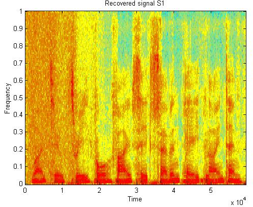
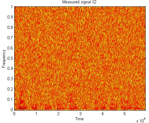
49 Speech from noise separation s x y 49/58

50 When does ICA work!? source signals s i (t) must be statistically independent. p ( s) = pi( si) source signals s i (t), except one, must be non-gaussian. mixing matrix A must be nonsingular and square. N i= C ( s ) 0 n> 2 n W i A 1 Knowledge of the physical interpretation of the mixing matrix is of crucial importance. 50/58

51 When does ICA work!? Ambiguities of ICA. a) Variances (energies) of the independent components can not be determined. This is called scaling indeterminacy. The reason is that both s and A being unknown any scalar multiplier in one of the sources can always be canceled by dividing the corresponding column of A by the same multiplier: 1 x= i a αi ( sα ) i i i b) Order of the independent components can not be determined. This is called permutation indeterminacy. The reason is that components of the source vector s and columns of the mixing matrix A could be freely changed in such that x=ap -1 Ps where P permutation matrix, Ps is new source vector with original components but in different order and AP -1 is a new unknown mixing matrix. 51/58

52 When does ICA work!? To illustrate ICA model in statistical terms we consider two independent uniformly distribute signals s 1 and s 2. Scatter plot on the left picture shows that there is no redundancy between them i.e. no knowledge could be gained about s 2 from s 1. Right picture shows mixed signals obtained according to x=as where A=[5 10;10 2]. Obviously there is dependence between x 1 and x 2. Knowing maximum or minimum of x 1 enables to know x 2 A could be estimated. But what if sources signals have different statistics? Source signals Mixed signals 52/58

53 When does ICA work!? Consider two independent source signals s 1 and s 2 generated by the truck and tank engines. Scatter plot on the left picture shows that there is again no redundancy between them i.e. no knowledge could be gained about s 2 from s 1. But distribution is different i.e. sparse. Right picture shows mixed signals obtained according to x=as where A=[5 10;10 2]. Obviously there is dependence between x 1 and x 2. But edges are at different positions this time. Estimated A from the scatter plot would be very unreliable. ICA can do that for different signal statistics without knowing that in advance. Source signals Mixed signals 53/58

54 When does ICA work!? Whitening is only half of the ICA. Whitening transform decorrelates signals. If signals are non-gaussian it does not make them independent. Whitening transform is usually useful first processing step in ICA. A second rotation stage achieved by an unitary matrix can be obtained by ICA exploiting non-gaussianity of the signals. Source signals Mixed signals Whitened signals 54/58

55 When does ICA work!? Why Gaussian variables are forbidden? Suppose two independent components s 1 and s 2 are Gaussian. Their joint density is given by s1 + s 2 1 s ps ( 1, s2) = exp = exp 2π 2 2π 2 Assume that source signals are mixed with orthogonal mixing matrix i.e. A -1 =A T. Their joint density is given by T 2 1 Ax T T 2 2 px ( 1, x2) = exp det A = A x = x anddet A = 1 2π x = exp 2π 2 Original and mixing distributions are identical there is no way that we could infer mixing matrix from the mixtures. 55/58

56 When does ICA work!? Why Gaussian variables are forbidden? Consider mixture of two Gaussian signals s 1 =N(0,4) and s 2 =N(0,9). After whitening stage scatter plot is the same as for source signals. There is no redundancy left after the whitening stage nothing for ICA to do. Source signals Mixed signals Whitened signals 56/58

57 When does ICA work!? PCA applied to blind image separation: z 1 z 2 MATLAB code: R x =cov(x ); % estimate of the data covariance matrix [E,D] = eig(r x ); % eigen-decomposition of the data covariance matrix Z = E *X; % PCA transform z =reshape(z(1,:),p,q); 1 % transforming vector into image figure(1); imagesc(z 1 ); % show first PCA image z 2 =reshape(z(2,:),p,q); % transforming vector into image figure(2); imagesc(z 2 ); % show second PCA image 57/58

58 Histograms of source, mixed and PCA extracted images Source image Mixed images PCA extracted images 58/58