An introduction to the Immersed boundary method and its finite element approximation

Transcription

1 FE An introduction to te and its finite element approximation Collaborators: Daniele offi, Luca Heltai and Nicola Cavallini, Pavia Pavia, 27 maggio 2010

2 FE History Introduced by Peskin Flow patterns around eart valves: a digital computer for solving te equations of motion <PD Tesis, 1972> analysis of blood flow in te eart <J. Comput. Pys., 1977> Extended by Peskin and McQueen since 83 to simulate te blood flow in a tree dimensional model of eart and great vessels Review article by Peskin Te immersed <Acta Numerica, 2002> Several applications in biology, wen a fluid interacts wit a flexible structure.

3 FE Main features Te structure is a part of te fluid wit additional forces and mass. Te Navier-Stokes equations are solved everywere. Te interaction wit te structure is obtained by means of a singular force term defined by a Dirac delta function. Te immersed material is modeled as a collection of fibers. Discretization based on finite differences.

4 FE FE discretization of IM <offi G., C&S 2003> <offi G. Heltai 2004, M3AS 2007> <offi G. Heltai Peskin CMAME 2008> <offi Cavallini G. 2010> of te FSI force No approximation of te Dirac delta function etter interface approximation (less diffusion, sarp pressure jump) Effective mixed finite elements for te approximation of te fluid equations. Submerged elastic solid occupying volume may also be considered.

5 FE elastic bodies Codimension 0 Codimension 1 t Elastic body Fluid body of codimension 0 te fluid domain and te immersed body ave te same dimension

6 FE elastic bodies Codimension 0 Codimension 1 t Elastic body Elastic t Fluid Fluid body of codimension 0 te fluid domain and te immersed body ave te same dimension body of codimension 1 te immersed body is eiter a curve in 2D or a surface in 3D

7 FE ω X(t) Notation Codimension 0 Codimension 1 t fluid + solid t deformable structure domain R d, d = 2, 3 t R m, m = d, d 1

8 FE ω X(t) Notation Codimension 0 Codimension 1 t fluid + solid t deformable structure domain R d, d = 2, 3 t R m, m = d, d 1 x Euler. var. in s Lagrangian var. in reference domain

9 FE ω X(t) Notation Codimension 0 Codimension 1 t fluid + solid t deformable structure domain R d, d = 2, 3 t R m, m = d, d 1 x Euler. var. in s Lagrangian var. in reference domain u(x, t) fluid velocity X(, t) : t position of te solid p(x, t) fluid pressure F = X deformation grad. (det F > 0) s

10 FE ω X(t) Notation Codimension 0 Codimension 1 t fluid + solid t deformable structure domain R d, d = 2, 3 t R m, m = d, d 1 x Euler. var. in s Lagrangian var. in reference domain u(x, t) fluid velocity X(, t) : t position of te solid p(x, t) fluid pressure F = X deformation grad. (det F > 0) s u(x, t) = X (s, t) were x = X(s, t) t

11 FE Codimension 0 Codimension 1 Case: m = d From conservation of momenta, in absence of external forces, it olds ( ) u ρ u = ρ t + u u = σ in In our case te Caucy stress tensor as te following form { σ f in \ t σ = σ f + σ s in t

12 FE Codimension 0 Codimension 1 Case: m = d From conservation of momenta, in absence of external forces, it olds ( ) u ρ u = ρ t + u u = σ in In our case te Caucy stress tensor as te following form { σ f in \ t σ = σ f + σ s in t Incompressible fluid: σ = σ f = pi + µ( u + ( u) T ) Visco-elastic material: σ = σ f + σ s wit σ s elastic part of te stress

13 FE Codimension 0 Codimension 1 Case: m = d From conservation of momenta, in absence of external forces, it olds ( ) u ρ u = ρ t + u u = σ in In our case te Caucy stress tensor as te following form { σ f in \ t σ = σ f + σ s in t Incompressible fluid: σ = σ f = pi + µ( u + ( u) T ) Visco-elastic material: σ = σ f + σ s wit σ s elastic part of te stress Moreover, if te structural material as a density ρ s different from te fluid density ρ f, we ave { ρ f in \ t ρ = ρ s in t

14 FE Codimension 0 Codimension 1 ρ f Virtual work principle u vdx + σ f : vdx σ f n vda = (ρ s ρ f ) u vdx σ s : vdx, t t v

15 FE Codimension 0 Codimension 1 ρ f Virtual work principle u vdx + σ f : vdx σ f n vda = (ρ s ρ f ) u vdx σ s : vdx, t t Te elastic stress σ s can be expressed in Lagrangian variables by means of te Piola-Kircoff stress tensor by: so tat ρ f P(s, t) = F(s, t) σ s (X(s, t), t)f T (s, t), u vdx + = (ρ s ρ f ) σ f : vdx t u vdx σ f n vda s P : s v(x(s, t)) ds v v

16 FE Codimension 0 Codimension 1 Using te Lagrangian description in te solid domain, te material derivative is te same as te time derivative, ence u = 2 X/ t 2. ρ f uvdx + σ f : v dx = (ρ s ρ f ) 2 X v(x(s, t)ds t2 P : s v(x(s, t)) ds

17 FE Codimension 0 Codimension 1 Using te Lagrangian description in te solid domain, te material derivative is te same as te time derivative, ence u = 2 X/ t 2. ρ f uvdx + σ f : v dx = (ρ s ρ f ) 2 X v(x(s, t)ds t2 At te end, after integration by parts, P : s v(x(s, t)) ds 2 X (ρ u σ f )v dx = (ρ s ρ f ) v(x(s, t)ds t2 + ( s P) v(x(s, t)) ds PN v(x(s, t)) da

18 FE Codimension 0 Codimension 1 From Lagrangian to Eulerian variables Implicit cange of variables using te Dirac delta function v(x(s, t)) = v(x)δ(x X(s, t)) dx

19 FE Codimension 0 Codimension 1 From Lagrangian to Eulerian variables Implicit cange of variables using te Dirac delta function v(x(s, t)) = v(x)δ(x X(s, t)) dx 2 X (ρ u σ f ) v dx = (ρ s ρ f ) v(x(s, t)ds t2 + ( s P) v(x(s, t)) ds PN v(x(s, t)) da

20 FE Codimension 0 Codimension 1 From Lagrangian to Eulerian variables Implicit cange of variables using te Dirac delta function v(x(s, t)) = v(x)δ(x X(s, t)) dx 2 X (ρ u σ f ) v dx = (ρ s ρ f ) v(x(s, t)ds t2 + ( s P) v(x(s, t)) ds PN v(x(s, t)) da substitute v(x(s, t)) 2 ( ) X = (ρ s ρ f ) t 2 v(x)δ(x X(s, t)) dx ds ( ) + ( s P) v(x)δ(x X(s, t)) dx ds ( ) PN v(x)δ(x X(s, t)) dx da

21 FE Codimension 0 Codimension 1 (ρ u σ f ) v dx 2 ( ) X = (ρ s ρ f ) t 2 v(x)δ(x X(s, t)) dx ds ( ) + ( s P) v(x)δ(x X(s, t)) dx ds ( ) PN v(x)δ(x X(s, t)) dx da

22 FE Codimension 0 Codimension 1 (ρ u σ f ) v dx 2 ( ) X = (ρ s ρ f ) t 2 v(x)δ(x X(s, t)) dx ds ( ) + ( s P) v(x)δ(x X(s, t)) dx ds ( ) PN v(x)δ(x X(s, t)) dx da and cange te order of te integrals 2 X = (ρ s ρ f ) δ(x X(s, t)) ds v dx t2 + ( s P)δ(x X(s, t)) ds v dx PNδ(x X(s, t)) da v dx

23 FE Codimension 0 Codimension 1 Since v is arbitrary, we get 2 X ρ u σ f = (ρ s ρ f ) δ(x X(s, t)) ds t2 + s Pδ(x X(s, t)) ds PNδ(x X(s, t)) da

24 FE Codimension 0 Codimension 1 Since v is arbitrary, we get 2 X ρ u σ f = (ρ s ρ f ) δ(x X(s, t)) ds t2 + s Pδ(x X(s, t)) ds PNδ(x X(s, t)) da Te source term can be split into tree contributions: excess Lagrangian mass density 2 X d(x, t) = (ρ s ρ f ) δ(x X(s, t)) ds t2 inner force density g(x, t) = s P(s, t)δ(x(s, t) x) ds and transmission force density t(x, t) = P(s, t)n(s)δ(x(s, t) x) ds

25 FE Codimension 0 Codimension 1 Strong Navier Stokes ( ) u ρ t + u u µ u + p = d + g + t in ]0, T [ div u = 0 in ]0, T [ Excess of Lagrangian mass and force densities in ]0, T [ 2 X d(x, t) = (ρ s ρ f ) δ(x X(s, t)) ds t2 g(x, t) = s P(s, t)δ(x X(s, t))ds t(x, t) = P(s, t)n(s)δ(x X(s, t))ds structure motion X (s, t) = u(x(s, t), t) in ]0, T [ t Initial and condition

26 FE Codimension 0 Codimension 1 ρ f u vdx + = (ρ s ρ f ) t t s ts/2 Case: m = d 1 Te domain occupied by te structure is t ] t s /2, t s /2[. Te pysical quantities depend only on te variables wic represent a middle section and are constant in te direction ortogonal to it. σ f : vdx t s/2 t u vd xdτ σ f n vda ts/2 t s/2 t σ s : vd xdτ

27 FE Codimension 0 Codimension 1 ρ f u vdx + = (ρ s ρ f ) t t s ts/2 Case: m = d 1 Te domain occupied by te structure is t ] t s /2, t s /2[. Te pysical quantities depend only on te variables wic represent a middle section and are constant in te direction ortogonal to it. σ f : vdx t s/2 t u vd xdτ = (ρ s ρ f )t s t u vd x t s σ f n vda ts/2 t s/2 t σ s : vd x, t σ s : vd xdτ

28 FE Codimension 0 Codimension 1 Working as before, we arrive at ρ f u σ f = (ρ s ρ f )t s + t s t s s Pδ(x X(σ, t))ds 2 X δ(x X(σ, t))ds t2 PNδ(x X(σ, t))da.

29 FE Codimension 0 Codimension 1 Working as before, we arrive at ρ f u σ f = (ρ s ρ f )t s + t s t s s Pδ(x X(σ, t))ds 2 X δ(x X(σ, t))ds t2 PNδ(x X(σ, t))da. Excess of Lagrangian mass and force densities in ]0, T [ 2 X d(x, t) = (ρ s ρ f )t s δ(x X(s, t)) ds t2 g(x, t) = t s s P(s, t)δ(x X(s, t))ds t(x, t) = t s P(s, t)n(s)δ(x X(s, t))da N: if is a closed curve in 2D or a closed surface in 3D ten is empty and te transmission force density τ vanises.

30 FE Codimension 0 Codimension 1 Strong Navier Stokes ( ) u ρ t + u u µ u + p = d + g + t in ]0, T [ div u = 0 in ]0, T [ Excess of Lagrangian mass and force densities in ]0, T [ 2 X d(x, t) = δρ δ(x X(s, t)) ds t2 g(x, t) = s P(s, t)δ(x X(s, t))ds t(x, t) = P(s, t)n(s)δ(x X(s, t))da δρ = { ρs ρ f if m = d (ρ s ρ f )t s if m = d 1 P = { P if m = d t s P if m = d 1. structure motion X (s, t) = u(x(s, t), t) in ]0, T [

31 FE Navier Stokes d ρ f (u(t), v) + a(u(t), v) + b(u(t), u(t), v) (div v, p(t)) dt 2 X = δρ v(x(s, t))ds+ < F(t), v > t2 v H0 1()d (div u(t), q) = 0 q L 2 0 () F(t), v = P(F(s, t)) : s v(x(s, t)) ds v H0 1 () d X (s, t) = u(x(s, t), t) t s u(x, 0) = u 0 (x) x, X(s, 0) = X 0 (s) s. a(u, v) = µ( u, v) b(u, v, w) = ρ f 2 ((u v, w) (u w, v))

32 FE Equivalence wit standard Te definition of g and t implies tat m = d g(x, t) = 0 for x t, t(x, t) = 0 for x t. Recall tat u(x(s, t), t) = 2 X. Ten te given Navier-Stokes t2 equations are equivalent to: ( ) u f ρ f t + uf u f σ f = 0 in ( \ t ) ]0, T [ ( ) u s ρ s t + us u s σ s f σs s = 0 in t ]0, T [ u f = u s on t ]0, T [ σ f f nf + σ s f ns = t (= F 1 PN) on t ]0, T [

33 FE Equivalence wit standard m = d 1 + t ( ) u ρ f t + u u µ u + p = 0 in ( + ) ]0, T [ u = 0 in ( + ) ]0, T [. ( [[ ]] u µ + [[p]]n n u = X t u + = u ) on t F = (ρ s ρ f )t s 2 X t 2 + t s s P on.

34 FE Incompressible and viscous yper-elastic materials X(t) t Trajectory of a material point X : [0, T ] t Deformation gradient F(s, t) = X (s, t) s Wide class of elastic materials are caracterized by: potential energy density W (F(s, t)) total elastic potential energy E (X(t)) = W (F(s, t))ds Piola-Kircoff stress tensor P(s, t) = W (s, t) ( F ) W inner force density s P(s, t) = s (F(s, t)) F

35 FE Recalling tat it olds X (s, t) = u(x(s, t), t) t s <offi Cavallini G. 10> ρ f 2 d dt u(t) 2 0 +µ u(t) d dt E(X(t))+ 1 2 δρ d dt X t 2 = 0 were E is te total elastic potential energy E (X(t)) = W (F(s, t)) ds

36 FE Fluid - Structure coupling Let t = f t s t be a time dependent region, wit f t fluid region, s t solid region in f t : incompressible Navier-Stokes equations wit Eulerian or ALE unknowns: velocity u and pressure p in s t: elastodynamics equation wit Lagrangian unknown: structure displacement η coupled troug transmission condition on Σ t = s t f t : continuity of velocities and stresses between fluid and structure

37 FE strategies for coupled problems Two approaces: <Matties-Niekamp 03> <Matties-Niekamp-Steindorf 06> Strongly coupled or monolitical Direct solution of te coupled problem. Stable but requires te solution of a big nonlinear problem. Weakly coupled or partitioned Separate solution of fluid and solid equations iteratively. Considerable reduction of computational cost, but undesirable instability effects.

38 FE Added-mass and partitioned procedure In coupled, te fluid acts over te structure as an added-mass at te interface. Wen ρ s ρ f (ρ s and ρ f solid and fluid density) te added-mass effect is negligible and standard partitioned procedures converge in few iterations. Te fails to converge wen ρ s /ρ f 1. <Nobile 01, Causin-Gerbeau-Nobile 05> Different strategies ave been proposed based on fully coupled implicit algoritms solved via iterative solvers using domain decomposition or algebraic splitting: <Le Tallec-Mouro 01, Deparis-Fernández-Formaggia 03> <adia-nobile-vergara 08, Giorda-Nobile-Vergara 09> <adia-quaini-quarteroni 08-09> or based on time-discretization via operator splitting: <Guidoboni-Glowinski-Cavallini-Canic 09>

39 FE Uniform background grid T for te domain (messize x ) Finite element approximation

40 FE Uniform background grid T for te domain (messize x ) Inf-sup stable finite element pair Finite element approximation V = {v H0 1()d : v Q2} Q = {q L 2 0 () : q P1}

41 FE Uniform background grid T for te domain (messize x ) Inf-sup stable finite element pair Finite element approximation V = {v H0 1()d : v Q2} Q = {q L 2 0 () : q P1} Grid S for (messize s )

42 FE Uniform background grid T for te domain (messize x ) Inf-sup stable finite element pair Finite element approximation V = {v H0 1()d : v Q2} Q = {q L 2 0 () : q P1} Grid S for (messize s ) Piecewise linear finite element space for X S = {Y C 0 (; ) : Y P1}

43 FE Uniform background grid T for te domain (messize x ) Inf-sup stable finite element pair Finite element approximation V = {v H0 1()d : v Q2} Q = {q L 2 0 () : q P1} Grid S for (messize s ) Piecewise linear finite element space for X S = {Y C 0 (; ) : Y P1} Notation T k, k = 1,..., M e elements of S s j, j = 1,..., M vertices of S E set of te edges e of S

44 FE Source term: F(t), v = Discrete source term P(F (s, t)) : s v(x (s, t)) ds v V

45 FE Source term: F(t), v = Discrete source term P(F (s, t)) : s v(x (s, t)) ds v V X p.w. linear F, P p.w. constant

46 FE Source term: F(t), v = Discrete source term P(F (s, t)) : s v(x (s, t)) ds v V X p.w. linear F, P p.w. constant y integration by parts M e F (t), v = P : s v(x(s, t)) ds T k k=1 M e = P Nv(X(s, t)) da T k k=1

47 [[P]] = P + N + + P N jump of P across e for internal edges [[P]] = PN jump wen e FE Source term: F(t), v = Discrete source term P(F (s, t)) : s v(x (s, t)) ds v V X p.w. linear F, P p.w. constant y integration by parts M e F (t), v = P : s v(x(s, t)) ds T k k=1 M e = P Nv(X(s, t)) da T k k=1 tat is F (t), v = [[P ]] v(x(s, t)) da e E e

48 FE Te semidiscrete problem becomes: find (u, p ) : ]0, T [ V Q and X : [0, T ] S suc tat d ρ f dt (u (t), v) + a(u (t), v) + b(u (t), u (t), v) dx i (div v, p (t)) = δρ [[P ]] v(x (s, t))da e E (div u (t), q) = 0 (t) = u (X i (t), t) dt u (0) = u 0 in X i (0) = X 0 (s i ) e i = 1,..., M 2 X t 2 v(x (s, t))ds i = 1,..., M v V q Q

49 FE Semidiscrete stability <offi Cavallini G. 10> ρ d 2 dt u (t) µ u (t) d dt E(X (t)) δρ d X 2 dt t = 0.

50 FE Fully discrete problem ackward Euler E Find (u n+1, p n+1 ) V Q e X n+1 S suc tat F n+1, v = [[P ]] n+1 v(x n+1 (s))da v V e E e NS ( u n+1 u n ρ f, v t (div v, p n+1 δρ ) ) = X n+1 + a(u n+1, v) + b(u n+1, u n+1, v) 2X n + Xn 1 t 2 v(x n+1 (s))ds + < F n+1, v > v V (div u n+1, q) = 0 q Q ; X n+1 i X n i t = u n+1 (X n+1 i ) i = 1,..., M.

51 FE Step 1. F n, v = e E Fully discrete problem Modified bckward Euler ME e [[P ]] n v(x n (s, t)) da v V Step 2. find (u n+1, p n+1 ) V Q suc tat ( ) u n+1 u n ρ f, v + a(u n+1 t, v) + b(u n+1, u n+1, v) (div v, p n+1 ) = NS X n+1 2X n δρ + Xn 1 t 2 v(x n (s))ds + F n, v v V (div u n+1, q) = 0 q Q ; Step 3. Xn+1 i X n i t = u n+1 (X n i ) i = 1,..., M.

52 FE Using Step 3 in Step 2 we arrive at: Step 1. F n, v = [[P ]] n v(x n (s, t)) da v e E e V Step 2. find (u n+1, p n+1 ) V Q suc tat ( ) u n+1 u n ρ f, v + a(u n+1 t, v) + b(u n+1, u n+1, v) (div v, p n+1 ) = NS u n+1 (X n δρ (s)) un (Xn 1 (s)) v(x n t (s))ds + F n, v v V (div u n+1, q) = 0 q Q ; Step 3. Xn+1 i X n i t = u n+1 (X n i ) i = 1,..., M.

53 FE Discrete Energy Estimate <offi Cavallini G. 10> Assumption Set H iαjβ = 2 W (F) F iα F jβ Tere exist κ min > 0 and κ max > 0 s.t. for all tensors E κ min E 2 E : H : E κ max E 2 Artificial Viscosity Teorem Let u n, pn and Xn be a solution to te FE-IM. Let Σ n be te sum of te kinetic and elastic energy: Σ n = ρ f 2 un 2 0, + δρ 2 X n X n 1 t 2 0, + E [X n ]. Ten Σ n+1 Σ n + (µ + µ a ) u n CFL Condition: µ + µ a > 0

54 FE E is unconditionally stable, wile ME requires te term µ a to be not too large µ a = κ max C (m 2) s (d 1) x t L n space dim. solid dim. 2 1 L n t C x s 2 2 L n t C x 3 2 L n t L n t Cx/ 2 s

55 FE = ]0, 1[ ]0, 1[, = [0, L] ρ s = ρ f P = κ X s experiments parameters partitioned into 16 by 16 subsquares discretized by 618 uniformly spaced nodes t =.01 V continuous piecewise biquadratics Q 2 Q discontinuous piecewise linears P 1 S continuous piecewise linears Programs written in C++ wit te support of deal.ii libraries. Pictures and movies obtained wit Matlab and IM Opendx.

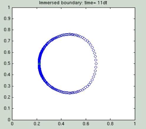
56 FE Ellipse immersed in a static fluid Aim: to examine te influence of te elastic force of te immersed on te wole system. Fluid initially at rest: u 0 = 0 ( 0.2 cos(2πs) X 0 (s) = 0.1 sin(2πs) ) s [0, 1], : time=0dt : time= 100dt

57 FE Percentage of area loss at t=2. M N = N = N = N =

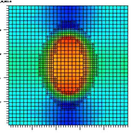
58 FE Structure model: Inflated baloon in a fluid at rest F (t), v = κ L Initial condition: ( R cos(s/r) X 0 (s) = R sin(s/r) Analytical solution: 0 2 X (s, t) s 2 v(x (s, t)) ds, κ = 1 ), s [0, 2πR] R = 0.4. u(x, t) = 0 x, t ]0, T [ p(x, t) = { κ(1/r πr), x R κπr, x > R t ]0, T [.

59 p FE Q2/P1 d solution Uniform grid: squares, t = 0.005, T = 3s Pressure on te cutline y= p p x Figure: Pressure Figure: Pressure cutline

60 FE P1isoP2/P1 c and P1isoP2/P1 c +P0 solutions Uniform grid: squares squares divided into two triangles t = , T = 0.1s Pressure P1isoP2/P1 c Pressure P1isoP2/P1 c +P0

61 FE P1isoP2/P1 c versus P1isoP2/P1 c +P0 cutline Uniform grid: squares divided into two triangles pressure q P1+P0 q P1 analytical 2

62 FE Area loss Uniform grid: squares divided into two triangles 1.2 x q P1 q (P1+P0) 1 A/A time

63 FE Examples of instability

64 FE Plot: µ a VS Σ n for different µ and t ρ f = 1, ρ s = 2, κ = 1, N=64, M=1024, 10 1 analysis η n Energy µ a = κc t s x L n 10 1 η n Energy µ = time time t = 10 1 t = η n 10 1 η n Energy Energy µ = time time

65 FE analysis for different ρ s ρ f = 1, µ = 0.1, κ = 1, N=64, M=1024, 10 1 η n Energy 10 1 η n Energy 10 1 η n Energy time time time 10 1 ρ s = 11 η n 10 1 ρ s = 1.1 η n 10 1 ρ s = 0.9 η n Energy Energy Energy time time time ρ s = 0.8 ρ s = 0.4 ρ s = 0.2

66 FE Some numerical experiments Equal densities Original 2D code in Fortran 77, ported to DEAL.II (c ++ ) ( by L. Heltai Rectangular mes, 2D - Codimension 1 Q2/P1 d 2D - Codimension 0 3D - Codimension 1

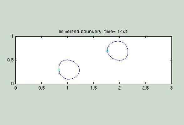
67 FE Some numerical experiments Different densities Original 2D code in Fortran 90 by N. Cavallini Triangular mes P1isoP2/P1 c Inflated balloon falling down in a liquid Densities: ρ s = 21 and ρ f = 1 κ = 1 κ = 0.1 κ = 0.1 κ = 1 κ = 0.1

68 FE Te is extended to te treatment of tick materials modeled by viscous-yper-elastic constitutive laws. Te case of fluid and structure wit different densities as been also considered. Te finite element approac is efficient and can easily andle te case of tick materials. analysis of te partitioned space-time discretization is provided. Te does not depend on te values of ρ f and of ρ s.