The Pennsylvania State University. The Graduate School. Department of Engineering Science and Mechanics ULTRASONIC GUIDED WAVE MECHANICS

Transcription

1 The Pennsylvania State University The Graduate School Department of Engineering Science and Mechanics ULTRASONIC GUIDED WAVE MECHANICS FOR COMPOSITE MATERIAL STRUCTURAL HEALTH MONITORING A Thesis in Engineering Science and Mechanics by Huidong Gao 7 Huidong Gao Submitted in Partial Fulfillment of the Requirements for the Degree of Doctor of Philosophy May 7

2 The thesis of Huidong Gao was reviewed and approved* by the following: Joseph L. Rose Paul Morrow Professor of Engineering Science and Mechanics Thesis Advisor Chair of Committee Bernhard R. Tittmann Schell Professor of Engineering Science and Mechanics Clifford J. Lissenden Associate Professor of Engineering Science and Mechanics Charles E. Bakis Professor of Engineering Science and Mechanics Qiming Zhang Distinguished Professor of Electrical Engineering Judith A. Todd Professor of Engineering Science and Mechanics P.B.Breneman Department Head Chair Head of the Department of Engineering Science and Mechanics *Signatures are on file in the Graduate School

3 iii ABSTRACT The ultrasonic guided wave based method is very promising for structural health monitoring of aging and modern aircraft. An understanding of wave mechanics becomes very critical for exploring the potential of this technology. However, the guided wave mechanics in complex structures, especially composite materials, are very challenging due to the nature of multi-layer, anisotropic, and viscoelastic behavior. The purpose of this thesis is to overcome the challenges and potentially take advantage of the complex wave mechanics for advanced sensor design and signal analysis. Guided wave mechanics is studied in three aspects, namely wave propagation, excitation, and damage sensing. A 6 layer quasi-isotropic composite with a [(/45/9/- 45) s ] lay up sequence is used in our study. First, a hybrid semi-analytical finite element (SAFE) and global matrix method (GMM) is used to simulate guided wave propagation in composites. Fast and accurate simulation is achieved by using SAFE for dispersion curve generation and GMM for wave structure calculation. Secondly, the normal mode expansion (NME) technique is used for the first time to study the wave excitation characteristics in laminated composites. A clear and simple definition of wave excitability is put forward as a result of NME analysis. Source influence for guided wave excitation is plotted as amplitude on a frequency and phase velocity spectrum. This spectrum also provides a guideline for transducer design in guided wave excitation. The ultrasonic guided wave excitation characteristics in viscoelastic media are also studied for the first time using a modified normal mode expansion technique. Thirdly, a simple physically based feature is developed to estimate the guided wave sensitivity to damage in composites. Finally, a fuzzy logic decision program is developed to perform mode selection through a quantitative evaluation of the wave propagation, excitation and sensitivity features. Numerical simulation algorithms are validated with both finite element analyses and laboratory experiments. For the quasi-isotropic composite, it is found that the ultrasonic wave propagation characteristics are not always quasi-isotropic. The directional dependence is very significant at high frequency and higher order wave modes.

4 iv Mode separation between Rayleigh-Lamb type and Shear Horizontal type guided waves is not possible. In addition, guided wave modes along one dispersion curve line could have a significant difference in wave structure. Therefore, instead of using traditional symmetric, antisymmetric, and SH notation, a new notation is used to identify the dispersion curves in a numerical order. Wave modes with a skew angle larger than 3 degrees can exist in a quasi-isotropic composite plate, which is validated by both FEM and experiment. At low frequency, the first wave mode has higher sensitivity than that of the third wave mode. However, the attenuation of the first wave mode is higher than that of the third wave mode. The mode selection trade-offs are evaluated and recommendations are provided for guided waves used in long range structural health monitoring.

5 v TABLE OF CONTENTS NOMENCLATURE...viii GLOSSARY AND ABBREVIATIONS...x LIST OF FIGURES...xi LIST OF TABLES...xxi ACKNOWLEDGEMENTS...xxii Chapter Introduction.... Problem statement.... Literature review Ultrasonic guided wave propagation in plates Guided wave excitation and scattering Experimental techniques in structural health monitoring of composites Summary of the literature review and challenges for further study....3 Thesis objectives A preview of the thesis content...4 Chapter Wave propagation theory in composite laminates...7. Problem formulation...7. The global matrix method The partial wave theory Boundary conditions and the global matrix method Wave field solutions....3 The semi-analytical finite element method Important derived guided wave properties Power flow and energy density Group velocity and energy velocity Skew angle Wave field normalization...3 Chapter 3 Guided wave propagation in quasi-isotropic composites A numerical model of composite laminates Phase velocity dispersion curves Group velocity and energy velocity dispersion curves Skew angle dispersion curves...45

6 vi 3.5 Wave structure analysis Summary...49 Chapter 4 Guided wave excitation in composites Theory The reciprocity relation and mode orthogonality The normal mode expansion technique Source influence on wave excitation Numerical proof of mode orthogonality in a quasi-isotropic laminate Wave mode excitability Numerical results of source influence Excitation signal analysis Transducer geometry and loading pattern influence Frequency and phase velocity spectrum of a finite source Guided wave dispersion Dispersion signal reconstruction Wave mode dispersion coefficient Guided wave field simulation Theory Wave field reconstruction case studies in composite laminates First fundamental wave mode The third fundamental wave mode Guided wave beam spreading analyses...9 Chapter 5 Finite element modeling of wave excitation and propagation Theory of a three dimensional FEM Wave excitation and propagation case studies in ABAQUS Case I: the first wave mode Case II: the third wave mode Case III: wave modes with large skew angle Summary...4 Chapter 6 Guided waves in composites considering viscoelasticity Dispersion relation derivation Numerical simulation results on wave propagation A new normal mode expansion technique for viscoelastic media Numerical simulation results Summary...7 Chapter 7 Guided wave sensitivity to damage in composites...9

7 7. Effect of material property degradation on guided wave propagation Theoretical study Density variation Elastic stiffness variation Ply thickness variation Guided wave scattering sensitivity Summary...4 Chapter 8 Guided wave mode selection Introduction Guided wave mode selection rules Guided wave long range monitoring potential...47 Chapter 9 Experimental studies Wave propagation study with contact transducers Ultrasonic transducers and instruments Experimental phase velocity dispersion curves Guided wave group velocity and attenuation studies Guided wave skew angle studies Wave excitation with piezoelectric active sensors Guided wave damage detection with piezoelectric active sensors Summary...7 Chapter Conclusions and discussions Summary of the thesis study Specific contributions Future work...78 References...79 Appendix A Guided wave imaging techniques in SHM...84 A. Signal processing and feature extraction...84 A. Guided wave imaging algorithms...85 A.3 Application of imaging techniques in laboratory experiments...87 A.3. E airplane wing crack monitoring...87 A.3. Helicopter component corrosion monitoring...88 A.3.3 Composite delamination monitoring...89 Appendix B Nontechnical abstract...9 vii

8 viii NOMENCLATURE Symbol Meaning c ijkl, c Elastic constant tensor C IJ, C Elastic constant in matrix format ' C '' C Elastic part of stiffness constant Viscous part of stiffness constant E, E, G, ν, ν 3 Engineering elastic constants of a composite lamina ρ t Density Time x i h i H u i, u v i, v σ ij, σ ε ij, ε S ij P i, P T i, F λ f ω c p c g Position Thickness of each ply Total thickness of the laminate Displacement Particle velocity Stress Strain Engineering strain Poynting s vector Traction Wavelength Frequency Angular frequency Phase velocity Group velocity

9 ix V e θ Φ ξ α β Energy velocity Propagation direction Skew angle Wave number Attenuation part of wave number Complex wave number P Wave mode orthogonality evaluation from complex mn reciprocity relation Q Wave mode orthogonality evaluation from real mn reciprocity relation B i, B D N M K Coefficient of partial waves in the global matrix method Global matrix in the global matrix method Shape functions in FEM Mass matrix in FEM Stiffness matrix in FEM

10 x GLOSSARY AND ABBREVIATIONS Name Explanation Dispersion coefficient An attribute of a wave mode describing its extent of dispersion Dispersion curve Energy velocity GMM Goodness Group velocity Mode sensitivity NDE NME Phase velocity RAPID SAFE SDC SHM Skew angle Source influence Wave excitability Wave structure A set of curves describing the wave mode dispersion relation of phase velocity, or some other feature, with respect to frequency Velocity of wave energy transmission Global matrix method An evaluation of a wave mode describing how much it satisfies a given set of criteria Velocity of wave package transmission An attribute of a wave mode describing its ability to detect a particular damage Nondestructive evaluation Normal mode expansion Velocity of a wave propagation with constant phase Reconstruction algorithm for probabilistic inspection of damage Semi-analytical finite element method Signal difference coefficient Structural health monitoring Angle between wave energy propagation and wave vector direction The influence of source geometry and signal on guided wave excitation An attribute of a wave mode describing its response to wave excitation Wave field profile along the thickness direction of a particular displacement, stress, energy, or other features.

11 xi LIST OF FIGURES Figure -: Materials on a Boeing 777 aircraft. (Courtesy NASA Langley Research Center)... Figure -: The trend of using composites in (a) military and (b) civil aircraft... Figure -3: Impact and fatigue damage to composite panels. (a) picture of a composite panel after low velocity impact (b) ultrasonic C-scan image showing internal delamination (c) fatigue damage to a composite plate... Figure -4: Concept of damage detection using guided waves. (a) pulse echo (b) through transmission...4 Figure -5: A vision of a Theoretically driven structural health monitoring strategy...5 Figure -: A coordinate system for wave mechanics study of a multi-layered structure...7 Figure -: A sketch of a one dimensional three node isoparametric element...4 Figure -3: A sketch of the power flow in a guided wave mode for the derivation of energy velocity....3 Figure -4: Sketch of slowness profile and skew angle. (Modified from [Rose 999])...3 Figure 3-: The sketches of the lay-up sequence and the wave propagation in a 6 layer quasi-isotropic composite laminate. Layup sequence is [(/45/9/-45) s ]..35 Figure 3-: A comparison of phase velocity dispersion curves obtained from two methods. Continuous lines: SAFE; Blue dots: GMM. Wave propagates in the o direction...36 Figure 3-3: Phase velocity dispersion curves for guided wave modes in different propagation directions. (a) mode, (b) mode (c) mode Figure 3-4: Angular profiles of the phase velocity dispersion curves at a frequency of khz, (a) mode (b) mode (c) mode 3. The units in the radius is km/s Figure 3-5: Phase velocity dispersion surfaces of the first three modes, (a) mode (b) mode (c) mode

12 Figure 3-6: Phase velocity dispersion surfaces of mode 4 to mode 6, (a) mode 4 (b) mode 5 (c) mode Figure 3-7: Comparison between the group velocity dispersion curves obtained from SAFE methods and energy velocity curves from the global matrix method. Continuous lines: SAFE; Blue dots: Global matrix method. Wave propagation in o direction...4 Figure 3-8: Mode group velocity dispersion curves for different propagation directions...43 Figure 3-9: Group velocity dispersion curves for different propagation directions and frequencies. (a) mode 3 (b) mode 4. Note: There are only four lines in (b) because. MHz is below the cut-off frequency of mode Figure 3-: Group velocity dispersion surface. (a) mode (b) mode...44 Figure 3-: A comparison between skew angle curves obtained from the SAFE and the GMM. Continuous lines: SAFE; Blue dots: GMM. Wave propagation in degree direction...45 Figure 3-: Variation of guided wave skew angle with respect to wave propagation directions. (a) mode -3 at khz (b) mode -4 at. MHz Figure 3-3: Skew angle surface of the first wave mode...46 Figure 3-4: A comparison of wave structures obtained from the GMM and the SAFE method. (a) displacement u, (b) stress σ Figure 3-5: Displacement and stress wave structure for the first wave modes at. MHz. (a) displacements (b) out of plane stress (c) in plane stress (d) power flow distribution...49 Figure 4-: Wave structure components for mode orthogonality validation. (a) v (b) v (c) v 3 (d) σ (e) σ (f) σ Figure 4-: Particle velocity spectrum in the x direction for the wave propagating in o at the surface of the [(/45/9/-45) s ] laminate....6 Figure 4-3: Rectified particle velocity spectrum for the wave propagating in o at the surface of the [(/45/9/-45) s ] laminate: (a) x direction, (b)x direction, (c) x 3 direction...6 xii

13 Figure 4-4: Angular profile of wave mode excitability (wave mode particle velocity at surface) for mode to mode 3 at khz. (a) shear (x direction) loading (b) normal (x 3 direction) loading....6 Figure 4-5: Phase velocity dispersion curves of guided wave propagation at o with the embedded information of wave mode excitability. Blue sections are most easily excited with shear loading in the x direction; red sections and black sections correspond to x and x 3 direction loading respectively Figure 4-6: Sample waveforms. (a) 5 cycled tone-burst signal with MHz center frequency and rectangular window, (b) 5 cycled tone-burst signal with MHz center frequency and Hanning window...64 Figure 4-7: Amplitude spectra of the 5 cycled tone burst signals with MHz center frequency.(a) Rectangular window, (b) Hanning window...65 Figure 4-8: Relation between bandwidth and center frequency under constant number of cycles (a) Rectangular window (b) Hanning window...66 Figure 4-9: Relation between bandwidth and center frequency under constant pulse width (a) Rectangular window (b) Hanning window...67 Figure 4-: Sketch of transducer loading model. (a) concentrated shear loading (b) concentrated normal loading (c) evenly distributed normal loading Figure 4-: Spatial domain loading distribution and its corresponding spatial frequency spectrum of a 3 element linear array with mm array element width. (a) concentrated shear loading (b) concentrated normal loading (c) evenly distributed normal loading....7 Figure 4-: Phase velocity spectrum for a 3 element linear array with mm array element width at MHz. (a) concentrated shear loading (b) concentrated normal loading (c) evenly distributed normal loading....7 Figure 4-3: Source influence spectrum of a 3 element transducer with mm element width and excited by a cycled tone burst signal with Hanning window and MHz center frequency. The loading is concentrated shear...7 Figure 4-4: Source influence spectrum of a 3 element transducer with mm element width and excited by a cycled tone burst signal with Hanning window and MHz center frequency. The loading is concentrated normal Figure 4-5: Source influence spectrum of a 3 element transducer with mm element width and excited by a cycled tone burst signal with Hanning xiii

14 window and MHz center frequency. The loading is evenly distributed normal...73 Figure 4-6: Reconstructed signals at mm, mm, mm, 3 mm, and 4 mm away from the excitation source. Source signal is a 5 cycle Hanning windowed tone burst with 5 khz center frequency. The wave mode considered is the first dispersion curve line for guided wave propagating in o of the [(/45/9-45) s ] laminate Figure 4-7: Reconstructed waveforms showing the effect of wave dispersion. Wave mode considered is the fifth mode line. The excitation signal is a 5- cycle Hanning windowed tone burst with 6kHz center frequency Figure 4-8: Sections of the phase velocity, group velocity dispersion curves for the fifth wave mode line along degree propagation direction. The amplitude spectrum of a 5-cycle Hanning windowed tone burst signal with 6 khz center frequency is also plotted Figure 4-9: First five dispersion coefficient lines for the wave propagation in the o direction of the [(/45/9/-45) s ] laminate Figure 4-: Mode selection results by the criterion of dispersion coefficient. (a) less than.µs/mm (b) larger than.5 µs/mm for the wave propagating in o direction of an [(/45/9/-45) s ] composite laminate. Blue dashed lines are the entire dispersion curve set. Red line sections are the modes that satisfy the criterion...8 Figure 4-: (Frequency)-(Phase velocity) spectrum of a 3 cycle khz signal with Hanning window on a mm wide element....8 Figure 4-: Wave mode component function of the wave field excited from a finite source listed in Tab Figure 4-3: u direction wave displacement at four positions...83 Figure 4-4: u 3 direction displacement at four positions...84 Figure 4-5: Wave field distribution along the thickness of the [(/45/9/-45) s ] structure. (a) u, (b) u Figure 4-6: Comparison between the wave field profile of the excited wave from a finite source with the wave structure at center frequency. The mode selected is the first mode at khz...86 Figure 4-7: Wave field snapshots at time equals to µs. (a) u, (b) u xiv

15 Figure 4-8: (Frequency)-(Phase velocity) spectrum of a 3 cycle khz signal with Hanning window on a 6 mm wide element using concentrated shear loading. Wave propagation direction is o...89 Figure 4-9: Wave mode component function of the wave field excited from a finite source listed in Tab Figure 4-3: Reconstructed wave signal at,, 4, 6 mm. (a) u, (b) u Figure 4-3: Wave field snapshots at a time of µs, (a) u, (b) u Figure 4-3: Skew angle and beam spreading curves of the first five wave mode lines. Structure: [(/45/9/-45) s ] laminate with. mm ply thickness. Wave vector direction: o...93 Figure 4-33: Mode selection results by the criterion of a beam spreading angle less than 5 o for the wave propagating in o direction of an [(/45/9/-45) s ] composite laminate. Blue dashed lines are the entire dispersion curve set. Red line sections are the modes that satisfy the criterion Figure 4-34: Mode selection results by the criterion of beam spreading angle larger than o for the wave propagating in o direction of an [(/45/9/- 45) s ] composite laminate. Blue dashed lines are the entire dispersion curve set. Red line sections are the modes that satisfy the criterion Figure 4-35: Beam spreading dispersion curves of the third mode line for four excitation wave vector directions. This shows the dependence of beam spreading on wave launching direction Figure 5-: A picture of a numerical model in ABAQUS used to efficiently excite the first guided wave mode at a khz center frequency...98 Figure 5-: A finite element mesh. (a) the entire model (b) a corner of the model... Figure 5-3: Top view of the wave field at µs. (a) u, (b) u Figure 5-4: Top view of the wave field at 4 µs. (a) u, (b) u Figure 5-5: Thickness profile of the guided wave at µs excited from a mm wide transducer element at khz. (a) u, (b) u 3... Figure 5-6: Wave signal comparison between the theoretical prediction from normal mode expansion and finite element modeling. (a) u, (b) u 3. The black box with dotted line shows the directly excited wave package....3 Figure 5-7: Wave field snapshots at µs. (a) u field, (b) u 3 field....5 xv

16 Figure 5-8: Wave field snapshots at µs: (a) u field, (b) u 3 field....6 Figure 5-9: Thickness profile of the guided wave at µs....7 Figure 5-: Wave signal comparison between the theoretical prediction from normal mode expansion and finite element modeling: (a) u, (b) u 3. Black box with dotted line: excited wave package....8 Figure 5-: Skew angle dispersion curve of wave propagation in o direction of a quasi-isotropic composite laminate....9 Figure 5-: Wave excitation (f-c p ) spectrum for a 5 element transducer with 3 mm element width and excited with a cycled signal at 7 khz using a Hanning window... Figure 5-3: Wave mode content curve for the loading described in Tab Figure 5-4: Sample wave field snapshots of u 3. (a).5 µs (b) µs... Figure 5-5: The displacement and power flow wave structures of the guided wave mode with large skew angle. The mode studied is the fifth wave mode at a frequency of.7 MHz....3 Figure 6-: (a) Phase velocity dispersion curve and (b) attenuation dispersion curves obtained from Hysteretic model...8 Figure 6-: (a) Phase velocity dispersion curve and (b) attenuation dispersion curves obtained from Kelvin-Voigt model...9 Figure 6-3: Wave modes with least attenuation at a given frequency. (a) Hysteretic model (b) Kelvin-Voigt model...9 Figure 6-4: Comparison of phase velocity dispersion curves between the elastic model and the Hysteretic viscoelastic model. Dotted line: elastic model, solid line: viscoelastic model. (a) full set of dispersion curve, (b) magnified curve shows mode interaction.... Figure 6-5: Wave structure comparison between the elastic model and the viscoelastic model. Wave mode: first mode at khz, u displacement. (a) real part (b) imaginary part... Figure 6-6: A comparison of energy velocity dispersion curve generated from the elastic and viscoelastic models. (a) elastic model (b) viscoelastic model.... Figure 6-7: Guided wave feature comparisons from a viscoleastic model. (a) Wave modes with largest group velocity for a given frequency (b) Wave modes with smallest attenuation for a given frequency...3 xvi

17 Figure 6-8: Comparison of skew angle dispersion curves obtained from elastic and viscoelastic models. Dotted line: elastic model. Solid line: Hysteretic viscoelastic model...3 Figure 6-9: Comparison of wave mode excitability with x direction force on the surface. Dotted line: Elastic model; solid line: Viscoelastic Hysteretic model. (a) frequency range of to MHz. (b) magnified region of mode interaction...6 Figure 6-: A comparison of wave mode excitability using F direction loading in (a) an elastic and (b) a viscoelastic model...7 Figure 7-: Dispersion curves for guided wave propagation in composite laminates. Blue dashed line: nominated mass density of IM7/977-3 ρ=.6 kg/m 3 Red line :assumed % density reduction ρ=.44 kg/m Figure 7-: Figure illustrates the effect of dispersion curve scaling when the material property degradation introduces % stiffness reduction. Blue dashed line: no stiffness reduction, blue solid line predicted dispersion curve with stiffness reduction, red dots calculated dispersion curve with stiffness reduction....3 Figure 7-3: Effect of engineering constant variation on guided wave dispersion curves. Blue dashed line: nominal material property. Red line: with % fiber direction modulus (E ) reduction of the lamina...33 Figure 7-4: Effect of engineering constant variation on guided wave dispersion curves. Blue dashed line: nominal material property. Red line: with % transverse modulus (E ) reduction of the lamina...34 Figure 7-5: Effect of engineering constant variation on guided wave dispersion curves. Blue dashed line: nominal material property. Red line with % in plane shear modulus (G ) reduction of the lamina Figure 7-6: Effect of engineering constant variation on guided wave dispersion curves. Blue dashed line: nominal material property. Red line with % Poisson s ratio(v ) reduction of the lamina Figure 7-7: Effect of engineering constant variation on guided wave dispersion curves. Blue dashed line: nominal material property. Red line with % Poisson s ratio (v 3 ) reduction of the lamina Figure 7-8: Variation of dispersion curves due to ply thickness change of a 6 layer quasi-isotropic composite. Blue lines:.mm Red lines:.8mm xvii

18 Figure 7-9: Effect of surface erosion on guided wave phase velocity dispersion of a 6 layer quasi-isotropic composite laminate. Blue line: all ply thickness. mm. Red line: first layer thickness reduction of. mm...37 Figure 7-: Estimated sensitivity spectrum of guided wave modes to delamination at the first laminate interface of a [(/45/9/-45) s ] composite structure Figure 7-: Estimated sensitivity spectrum of guided wave modes to delamination at the 3rd laminate interface of a [(/45/9/-45) s ] composite structure....4 Figure 7-: Estimated sensitivity spectrum of guided wave modes to delamination in a [(/45/9/-45)s] composite structure...4 Figure 8-: Goodness function definition for guided wave selection. Evaluates attenuation characteristic (a) Crisp rule (b) fuzzy rule Figure 8-: Mode selection results considering wave mode attenuation. (a) Crisp mode selection with.5db/mm allowed. (b) Fuzzy selection...45 Figure 8-3: The mode selection rule and candidate wave modes for large skew angle demonstration. (a) High pass filter for the absolute value of skew angle. (b) Mode selection results...46 Figure 8-4: Guided wave mode selection for the purpose of demonstration large skew angle Figure 8-5: Guided wave mode selection considering attenuation. (a) selection rule (b) selection result Figure 8-6: Guided wave mode selection considering mode dispersion. Less dispersive modes selected (a) selection rule (b) selection results...49 Figure 8-7: Guided wave mode selection considering mode sensitivity (a) selection rule (b) selection result Figure 8-8: Guided wave mode selection considering wave excitation with loading in the x direction. (a) Selection rule (b) qualified wave modes plotted in red....5 Figure 8-9: Guided wave mode selection considering wave excitation with loading in the x 3 direction. (a) Selection rule (b) qualified wave modes plotted in red....5 xviii

19 Figure 8-: Overall guided wave mode selection considering rules to 4 listed in Tab Figure 9-: Test setups for ultrasonic guided wave propagation study Figure 9-: Integrated ultrasonic testing system...53 Figure 9-3: Guided wave signal collected at mm position, when the transmitter is at from the left edge...54 Figure 9-4: Ultrasonic guided wave phase velocity dispersion curve for wave propagating in the o of a quasi-isotropic composite laminate. Wave mode lines are numbered on the dispersion curves Figure 9-5: Guided wave signals collected from a linear scan showing edge multi-mode, edge reflection, and complex interference. (a) Experimental signals. (b) sketch of the first few wave paths. (): direct transmission mode 3, () Reflected mode three from left edge, (3) reflected mode 3 from right edge, (4) direct through transmission of mode...56 Figure 9-6: Frequency and phase velocity spectrum of guided wave signals shown in Fig Figure 9-7: A comparison between the experimental dispersion curve and theoretical dispersion curve for wave propagation along the degree direction Figure 9-8: Comparison of guided wave modes in the experiment with theoretical expectation using low attenuation, low skew angle, and excitable rules, and frequency spectrum of source influence. The result shows that the experiment meets the expectation...6 Figure 9-9: Guided wave signals from a 8kHz transducer. (a) Illustration of guided wave phase velocity and group velocity in a wave package. (b) frequency and phase velocity spectrum...6 Figure 9-: Energy content in the guided wave signal as a function of position showing wave attenuation...6 Figure 9-: Experiments to test the effect of energy skew in a quasi-isotropic composite plate Figure 9-: Guided waves excited from angle wedge to validate the concept the concept of large skew angle. The black line at the center corresponds to the xix

20 wave launching direction. The line in -6 mm position marks the position where a maximum signal is detected Figure 9-3: Guided wave signals from surface mounted piezoelectric transducers. Excitation signal khz, pulse width 5 µs. transducer element widths: (a) 4mm, (b) 6mm, and (c) 8mm...66 Figure 9-4: Expected guided wave modes from a surface excitation source. Excitation signal has center frequency khz and cycles...67 Figure 9-5: Picture of a plastic put on the top of a composite plate to simulate damage. Plastic putting dimensions: mm x mm x5 mm...68 Figure 9-6: Guided wave signals (a) before damage, (b) after damage, and (c) the difference of the signals in (a) and (b). Transducer: 4mm width. Excitation signal. khz with 5 µs pulse width...69 Figure 9-7: Guided wave signals (a) before damage, (b) after damage, and (c) the difference of the signals in (a) and (b). Transducer: 8mm width. Excitation signal. khz with 5 µs pulse width....7 Figure 9-8: Guided wave signals (a) before damage, (b) after damage, and (c) the difference of the signals in (a) and (b). Transducer: disc. Excitation signal. 35 khz with 5 µs pulse width....7 Figure A-: Concept of a ray affect area in RAPID reconstruction...86 Figure A-: Piezoelectric sensors on an aircraft wing panel Figure A-3: Reconstruction results from 5 micro pulse width data with adaptive threshold. (a) Reference state, (b) mm defect, (c) 3mm defect, (d) 4mm defect...88 Figure A-4: (a) Simulated corrosion damage in an helicopter component, Corrosion thickness / inch, area x. and (b) damage monitoring results with ultrasonic guided waves and RAPID reconstruction technique...89 Figure A-5: (a) Sensor array on a composite panel for impact damage detection, (b) sample signals before and after impact showing damage detection....9 Figure A-6: Impact damage localization with (a) ultrasonic C-scan (b) guided wave monitoring with RAPID algorithm....9 xx

21 xxi LIST OF TABLES Table 3-: Material properties of IM7/977-3 unidirectional composite properties...35 Table 3-: Phase velocity values at low frequency limit of the dispersion curves ( khz)...37 Table 4-: Wave mode orthogonality validation table...58 Table 4-: Comparison of theoretical velocities with the velocity values obtained from the reconstructed signals...77 Table 4-3: A loading design to efficiently excite the first fundamental wave mode...8 Table 4-4: A loading design to efficiently excite the third fundamental wave mode..88 Table 5-: Model and loading parameters in a finite element simulation...99 Table 5-: A finite element model parameters to excite the 3 rd wave mode...4 Table 5-3: Model geometry and loading pattern to demonstrate large skew angle... Table 6-: Lamina properties of the IM7/977-3 composite used in simulation...7 Table 8-: Proposed mode selection rules for mode selection based on long range delamination detection in composite laminates...48 Table 9-: Quantitative comparison of wave mode attenuation...6

22 xxii ACKNOWLEDGEMENTS I would like to take this opportunity to express my sincere thanks to my advisor, Dr. Joseph L. Rose, for his guidance and encouragement during the course of my study in the Pennsylvania State University. His valuable advice and philosophy on technical as well as personal matters will be a great treasure in my future career and life. I am also indebted to all other members of my doctoral committee, Dr. Bernhard Tittmann, Dr. Charles Bakis, Dr. Clifford Lissenden, and Dr. Qiming Zhang for their help in my research and suggestions on the improvement of this thesis. Thanks will also be given to FBS. Inc, Intelligent automation Inc., and NAVAIR, USA, for financial support in the research projects over the years, American society for nondestructive testing for a fellowship support, and GE Inspection Technologies for technical support in my study. I have also benefited from many colleagues in the Ultrasonic NDE lab and friends in Penn State. Thanks a lot for all of their helps in experiments and computations, valuable discussions, technical support, and finally valuable comments during this thesis preparation. Finally, sincere thanks are given to my parents for their support and understanding all along the path of my education. I would like to dedicate this thesis to my lovely wife, Guangfei, thank her for the support and sharing of my happiness and difficulties.

23 Chapter Introduction. Problem statement Fiber reinforced polymer composites are finding increased applications in the aircraft and aerospace industries due to their superior mechanical properties and light weight. Fig. - shows an example of the application of graphite fiber reinforced composites in a Boeing 777 aircraft [Chambers 3]. The application of composites in military aircraft is even more common than its use in commercial aircraft. The trends of increased use of composites in military and civil aircraft are illustrated in Fig. - [Chambers 3]. It shows that about 4% of the weight in a Lockheed F- aircraft is made of composite materials. The new Boeing 787 aircraft under development will have 5% of composite usage. In addition, a composite fuselage will be used for the first time in commercial aircraft. Figure -: Materials on a Boeing 777 aircraft. (Courtesy NASA Langley Research Center)

24 6 Weight percent of composite F-4 F-8 F-5 F-6 AV-8B F Year of first flight (a) Weigt percentage of composite 5 A3 A3 A3 A33 A A MD-9 DC DC Year of first flight Figure -: The trend of using composites in (a) military and (b) civil aircraft (b) (a) (b) (c) Figure -3: Impact and fatigue damage to composite panels. (a) Picture of a composite panel after low velocity impact (b) Ultrasonic C-scan image showing internal delamination (c) fatigue damage to a composite plate.

25 3 Despite their strength and low weight, composite materials are subject to damage during fatigue, mechanical impact, and aging in a service environment. As a simple example, dropping a ball on a composite plate might cause its fibers to break, the matrix to crack, and delamination to occur between the layers. Fig. -3 (a) shows a photo of a composite panel after low velocity impact. Although the damage is invisible at the surface, a big delamination occurs within the panel. Fig. -3 (b) shows the image of the delamination detected using a high frequency ultrasonic c-scan system [Bell 4]. Fig. -3 (c) shows an image of a composite panel after a laboratory fatigue test [Lissenden et al. 6]. Fiber breaking and delamination at the top surface can be clearly observed. These experiments were carried out in the Ultrasonic NDE lab at Penn State University in collaboration with the Composite Manufacturing Technology Center for composite panel preparation, the Engineering Nano Characterization Center for C-scan imaging, and the Axial-Torsion Fatigue Lab for fatigue testing. Damage in military aircraft and rotorcraft are even more serious due to erosion in harsh environments, ballistic impact, and fatigue. If the composite material is damaged, immediate repair would be required. Otherwise, these damages might lead to malfunctioning or even catastrophic failure of the aircraft. Traditionally, nondestructive evaluation (NDE) techniques are used to inspect the structures on a periodic basis. However, significant damages to the structure could occur during the intervals between inspections. Therefore, to provide early warning and timely detection of damage, real time structural health monitoring (SHM) techniques are greatly needed. Several methods currently under intensive research are vibration based methods, fiber optic based methods and electromechanical impedance based methods, and ultrasonic guided wave based methods. Ultrasonic guided waves are the mechanical waves propagating along the structure under the guidance of its boundaries. In structural health monitoring, waves are usually excited with surface mounted or embedded piezo-electric transducers. They propagate along the structure. The existence of damage and material degradation can be detected by evaluating the guided wave signals. Fig. -4 shows the concept of active damage detection using guided waves. Fig. -4 (a) is the pulse echo scenario, where a

26 4 single sensor is used in both wave generation and receiving. Fig. -4 (b) is the through transmission scenario, where a second transducer is used to receive the signal (from [Gao et al. 6] ). Sensor damage (a) Actuator damage Sensor (b) Figure -4: Concept of damage detection using guided waves. (a) pulse echo (b) through transmission. Besides the guided wave based method, some other methods are also under research and development for structural health monitoring. These include localized monitoring methods such as electromechanical impedance based methods, fiber optical methods, and global vibration based methods such as frequency transfer function and vibration mode shape analyses. Compared with localized monitoring, the ultrasonic guided wave based method has the capability of monitoring a larger area with a few sensors. Compared with the global vibration based technologies, ultrasonic guided waves can provide better sensitivity to localized damage. Therefore, it has great potential for applications in structure health monitoring.

27 5 Figure -5: A vision of a Theoretically driven structural health monitoring strategy Fig. -5 shows our PSU vision of a Theoretically driven structural health monitoring design and process based on ultrasonic guided waves. The entire process is divided into four levels, namely structural level, system level, sensor level, and physical level. In the design phase, the structural level health monitoring requirements are input into system level, sensor level, and physical level. In addition, the structural and material properties are used in a physical level guided wave mechanics study. The results of the guided wave mechanics studies are used for sensor, sensor network design, and optimized testing design. The information from the sensor design will also be used in the system level design. During the monitoring phase, excitation signals are sent out from monitoring systems to sensors. The information of structural integrity carried in the guided wave signal is collected with the sensors. Signal processing and decision making is then carried out in the system level. Finally, a health assessment of the structure is reported to meet the monitoring requirements. Since the use of ultrasonic waves to interrogate damage is the basis of the entire process, an understanding of ultrasonic guided wave propagation, excitation, and damage interrogation mechanisms is critical for the advancement of the technology.

28 6. Literature review A literature survey is presented on the subjects of ultrasonic guided wave mechanics and the current practice of ultrasonic guided wave based structural health monitoring. Since the objective of this study is more theoretically oriented, the literature survey therefore has an emphasis on the theoretical and numerical aspects of wave mechanics. In Section.., early studies of guided waves, ultrasonic waves in multilayered media, and waves in composite materials are reviewed. Studies on guided wave excitation and scattering are reviewed in Section... The state of the art of experimental studies in structural health monitoring using guided waves is reviewed in Section..3. Based on these reviews, challenges to guided wave study in composite structures are summarized in Section Ultrasonic guided wave propagation in plates Theoretical studies of ultrasonic guided waves can be retrieved back to a century ago when Lord Rayleigh [Rayleigh 885] studied surface acoustic waves. After that, waves in isotropic plates, waves at solid-solid and solid-liquid interface were studied by Lamb [Lamb 97], Stoneley [Stoneley 94], and Scholte [Scholte 94] respectively. All these wave types considered in the early studies have their displacement in the sagittal plane, which is a plane consisting of the wave propagation and thickness directions. In later research, these types of guided waves are generally referred to as Rayleigh-Lamb type waves. Another type of wave is called a shear horizontal (SH) wave, whose displacement is perpendicular to the sagittal plane. Love studied the shear horizontal waves in a layer on half space, which was later called a Love wave [Love 9]. Beyond these classic guided wave types, guided waves in other fundamental geometries, such as rods and hollow cylinders, were also studied. They can be found in these classical and recent text books [Victorov 967; Achenbach 973; Graff 973; Auld 99; Rose 999].

29 7 Ultrasonic bulk wave propagation in isotropic media can be studied using a Helmholtz decomposition or a partial wave theory. However, analytical solutions of wave propagation in an anisotropic media can only be studied using the partial wave technique. In a multi-layered media, the boundary conditions and interface conditions can be formulated in two different ways using the partial wave technique. One is a transfer matrix method, which is first developed by Thomson in 95 and later refined by Haskell [Thomson 95; Haskell 953]. In this method, a matrix is used to express the wave field on the top surface of a layer as a function of the field at the bottom surface. A transfer matrix, obtained by multiplying the matrices in all the layers, is used to describe the relationship between the wave field at the bottom and the top surfaces of the multilayered structure. The final size of the transfer matrix does not increase with the number of layers in the structure. Therefore, the transfer matrix method is efficient for structures with many layers. However, it suffers from numerical instabilities when the product of frequency and thickness is large. Dunkin used a delta operator method to alleviate the numerical instability of the transfer matrix method [Dunkin 965]. The other method is called a global matrix method first used by Knopoff [Knopoff 964]. A single matrix is used to assemble all the interface and boundary conditions together. This method does not have the numerical instability problem as in the transfer matrix method. However, the global matrix method can be computationally expensive especially when the number of layers is large. Around the 99s, studies on material property characterization for composites using ultrasonic bulk waves have accelerated the theoretical study of wave propagation in multilayered media. Nayfeh [Nayfeh 995] provided a standard solution for transfer matrix methods in generally anisotropic multilayered media. Experimental works were carried out on the bulk wave transmission and reflection in unidirectional composites, and cross ply composites [Chimenti D.E. 99; Nayfeh et al. 99]. Hosten, Tittmann, and Castaings applied the transfer matrix method in viscoelastic material characterization and bulk wave transmission and reflection studies in unidirectional, cross ply, and quasiisotropic composites [Hosten et al. 987; Hosten 99; Hosten et al. 993]. They also improved the delta operator method in the transfer matrix method [Castaings et al. 994].

30 8 Recently, as modifications to the transfer matrix method, compliance matrix and stiffness matrix methods were developed [Rokhlin et al. ]. The development of the transfer matrix method and global matrix method for bulk wave propagation in composite materials were also adapted for leaky guided wave analysis in composites. Mal generalized the global matrix method for guided waves in anisotropic media [Mal 988]. Chimenti and Nayfeh also studied the leaky Lamb waves in composite materials including the wave propagation in a [ /9 ] cross ply composite. Their experimental results matched well with numerical predictions for the waves propagating in directions with structural symmetry. However, the reflection spectra in non-symmetric directions do not match very well with the numerical expectation by missing predicted reflection minimums. The authors attributed this discrepancy to the coupling of wave displacements in three directions [Nayfeh 995]. To be more specific, we think that this should be related to the energy skew of the guided waves. Leaky guided waves in composites were also studied by many other researchers; details can be found in [Dayal et al. 989; Yoseph Bar-Cohen et al. 998] and the review paper by Chimenti [Chimenti 997]. A comprehensive review and comparison of the transfer matrix method and the global matrix method for guided waves in multi-layered structures can be found in Lowe [Lowe 995]. The global matrix method formulation with an emphasis for guided wave modal analysis used for long range NDE is addressed in detail in [Rose 999]. Besides the analytical models, a semi analytical finite element method (SAFE) is also used to simulate guided wave propagation. The SAFE method was used for the first time to study propagating wave modes in an arbitrary but uniform cross section in 973 [Lagasse 973]. In the SAFE method, the cross section of the waveguide is discretized with finite elements and an analytical solution is assumed in the wave propagation direction. After applying boundary conditions, dispersion curves describing wave propagation mode possibilities can be obtained. After that, the SAFE method is used by Dong and his colleagues to calculate both propagation and evanescent guided wave modes in anisotropic cylinders [Huang et al. 984]. Datta and his colleagues used the SAFE method for cross ply composite plates considering wave propagation in the

31 9 structural symmetry direction [Datta et al. 99]. Recently, the SAFE method was used by Garvric, Hayashi, Rose and Lee to study the wave propagation in rods, rails, and pipes [Gavric 995; Hayashi et al. 3; Lee 6]. Lanza di Scalea and his colleagues extended the SAFE method for guided waves in composites considering material damping effect [Matt et al. 5; Bartoli et al. 6]. Compared with the transfer matrix method, the SAFE method does not have the problem of numerical instability. In addition, the solution of guided wave dispersion curve is obtained by solving an eigenvalue problem. Therefore, complicated route searching is avoided in SAFE, and thus eliminated the problem of possible missing roots in matrix based methods. Another advantage of the SAFE method is its easy extension from an elastic model to a viscoelastic model as compared with a two dimension root searching method in matrix based methods... Guided wave excitation and scattering Analytical methods for solving ultrasonic guided wave excitation problems generally falls into two categories, one is an integral transform method and the other is a normal mode expansion technique. The integral transform method is studied by transforming the excitation source into frequency and wavenumber domain. After a harmonic system of equations with source terms is solved, the results are transformed back into time and spatial domain. The integral transform method is discussed in [Rose 999] for shear horizontal guided wave excitation in an isotropic plate. Recently, Giurgiutiu [Giurgiutiu 5] used the integral transform method to study Lamb wave excitation in an aluminum plate. The frequency tuning effect of guided wave excitation is also investigated. [Raghavan et al. 5] extended the integral transform method into a three dimensional analysis of guided wave excitation in isotropic plates. Mal and his students studied the wave excitation phenomenon in unidirectional and cross ply composites from a localized source especially to simulate the process of impact and acoustic emission effects using the global matrix method and simplified models using plate theory [Lih et al. 995; Mal ; Banerjee et al. 5]. Although the integral

32 transform method can be used to analyze wave excitation from localized sources, the inverse process of the integral transform is usually very difficult. In addition, the formulation of the integral transform method is usually very cumbersome. The normal mode expansion (NME) technique is based on a reciprocity relation in dynamics. The basic idea of NME is to express the actual wave field as a superposition of orthogonal guided wave mode solutions. The general theory of NME in an elastic and piezoelectric plate is described in a classic textbook by Auld [Auld 99]. Ditri and Rose used the NME technique for guided wave excitation in isotropic plates and pipes [Ditri et al. 99; Ditri et al. 994]. These analyses are later used as a basis for guided wave natural focusing and phased array focusing in pipes. The normal mode expansion technique is closely related to the guided wave propagation mode analysis. Compared with the integral transform method, a direct physical insight can be obtained from the process of normal mode expansion. The guided wave scattering problem is a very important yet difficult problem for NDE and SHM. Analytical study of guided wave scattering was introduced with an S- parameter technique in [Auld 99]. In the past two decades, more and more research on wave excitation and scattering were carried out using numerical methods such as the finite difference method (FDM), the boundary element method (BEM), and the finite element method (FEM). Among a large amount of numerical simulations on wave scattering, some typical ones related to guided waves in composites are reviewed in the following. A two-dimensional finite element method for wave propagation and scattering study in composites was presented by Cawley and Guo [Guo et al. 993]. A numerical simulation tool based on the finite different method called LISA was developed and used to simulate the wave propagation and scattering in a composite plate [Agostini et al. 3; Lee et al. 3; Lee et al. 3]. Recently, commercial finite element software packages, such as ABAQUS and ANSYS, are also used in the simulation of ultrasonic guided waves in many structures including composites [Su et al. 4; Yang et al. 6]. Although these finite element methods can be used to calculate the guided wave field in composites, these methods are computationally expensive and usually difficult for handling large structures. In order to combine the benefit of numerical methods for

33 scattering field calculation and analytical techniques for a physical understanding of guided waves, a hybrid BEM and NME technique was used by Rose and his colleagues for isotropic plate structures [Cho et al. 996; Cho ; Zhao et al. 3]. A similar method of combining NME with the FEM was recently used to simulate guided wave excitation in a unidirectional composite plate [Moulin et al. ]...3 Experimental techniques in structural health monitoring of composites Several decades ago, the need for nondestructive evaluation of composite materials accelerated the analytical and numerical research of ultrasonic wave propagation in multi-layered structures. As a result, this research has benefited the NDE applications with new techniques using bulk waves and leaky lamb waves. In addition, to water immersion tests, recently air coupled transducers were also used for nondestructive evaluation of composites. In recent years, the demand of condition based maintenance has created the need for real time structural health monitoring and assessment using permanently attached sensors. The research emphasis is turning toward guided wave monitoring using active and passive sensing due to its long range monitoring capability. Surface attached and embedded piezoelectric elements have become a common practice for structural health monitoring of metallic and composite structures. A detailed review of experimental techniques can be found in [Sohn et al. 3; Staszewski et al. 4]. Although a detailed review is beyond the scope of this thesis, a non-comprehensive list of research groups with great contributions in this field are Chang at Stanford University, Giurgiutiu at University of South Carolina, Inman at Virginia Tech, Boller at Sheffield University, and Sohn at Carnegie Mellon. Chang and his colleagues developed a SMART layer concept with piezoelectric disc elements integrated in a polyimide substrate, such that they can be easily applied to both metallic and composite structures [Lin et al. ]. Giurgiutiu and his students studied the electromechanical impedance method for damage detection in metallic aircraft panels using piezoelectric wafers [Giurgiutiu et al. 5]. In addition, they studied the lamb wave excitation in isotropic plates [Giurgiutiu 5] and developed

34 piezoelectric sensor phased arrays for guided wave beam steering in an isotropic plate [Giurgiutiu et al. 4]. The SMART layer as well as the individual piezoelectric wafer sensors have been used in many applications including composite plates. Many intelligent signal processing and statistical analysis techniques have been explored by these researchers [Staszewski ; Staszewski et al. 4; Yu et al. 5]. Although there is a trend of increased consideration of ultrasonic guided wave mechanics in these experiments, the application of guided wave mechanics in the SHM of composites is still desperately needed...4 Summary of the literature review and challenges for further study Despite the great application needs, the study of guided wave mechanics in composite materials still remains very challenging due to the following reasons.. Previous studies in composite materials are mostly in bulk wave propagation and a leaky wave point of view. Mode analyses for long range guided wave propagation in composites are very few.. Previous guided wave studies are mostly on isotropic structures or anisotropic structures with wave propagation in structural symmetry directions. Therefore, Rayleigh-Lamb (R-L) type waves are well separated from the shear horizontal (SH) waves. The guided wave mode notation, SH, A and S, are used to denote wave mode lines with shear horizontal, antisymmetric R-L, and symmetric R-L waves. However, for composite materials with general lay-ups, no distinct separation of R-L and SH type waves is guaranteed. No structural symmetric direction for wave propagation is guaranteed. No symmetric plane in the thickness direction is guaranteed. Therefore, the SH, A, and S notation system will no longer be universally applicable. In addition, guided wave modes along a single dispersion curve line could exhibit significantly different behaviors.

35 3 3. The complexities of guided wave propagation are significantly related to the composite lay-up sequence. Unidirectional and cross ply composites are studied in some previous works. However, only a few works are reported on guided waves in composite materials with other stacking sequences. 4. The energy skew effect is very important in guided wave propagation in anisotropic media, especially composites. However, to the best of our knowledge, no result is reported on the consideration of guided wave skew angle except for unidirectional composites. 5. Viscoelasticity of composite materials will significantly affect long range guided wave propagation potential. In previous literature, viscoelasticity is considered in guided wave propagation using the semi-analytical finite element method. However, the study of the viscoelastic effect on guided wave excitation is not reported. A new theoretical derivation is required to solve this problem. 6. In order to apply guided wave mechanics as a natural constitution of a structural health monitoring system, the research of guided wave mechanics should reach out from complicated mathematics formula to easily controllable design features, such as the evaluation of the extent of dispersion, extent of skew, and extent of attenuation of a guided wave mode..3 Thesis objectives The objective of this study is to provide a set of simulation methods and tools to integrate ultrasonic guided wave studies into the theoretically driven structural health monitoring strategy. For the wave mechanics community, the outcome of this study will be a deeper understanding of wave propagation and excitation characteristics in composites. For the structural health monitoring community, the outcome will be some

36 4 useful tools for sensor design and signal analysis. These tools are also applicable to other complex structures involving material anisotropy, multiple-layers, and viscoelasticity. Specific objectives of the research, aimed at conquering the challenges just listed, are as follows.. Develop computer programs to study the guided wave propagation in a composite structure with an arbitrary lay-up sequence. Use a quasiisotropic composite plate as a specific example.. Study the skew angle effect of wave propagation in composite plates. 3. Develop computer programs to study the wave excitation principles in composite laminates. Use the quasi-isotropic laminate as an example. 4. Derive a new theoretical procedure for the wave excitation study in composites considering material viscoelasticity and implement the new procedure into computer programs. 5. Develop simple physically based features to evaluate wave dispersion, excitation, and sensitivity. 6. Comprehensively consider all possible features for guided wave mode selection and to provide a mode selection framework that is directly applicable to structural health monitoring design. 7. Develop computer programs for sensor design to achieve appropriate mode selection and mode control. 8. Use FEM simulation and experiments to validate the performance of the simulation tools..4 A preview of the thesis content This thesis contains chapters and two appendices. Chapter presents the problem statement of guided wave mechanics studies in composites, a literature review, and a description of the thesis objectives. Chapter introduces the theories of the global matrix method and the semianalytical finite element method in elastic composite laminates. Guided wave mode

37 5 characteristics including phase velocity, group velocity, energy velocity, skew angle, displacement and stress distributions, power flow and energy distributions are defined. Chapter 3 studies the guided wave propagation in a 6 layer quasi-isotropic composite plate with [(/45/9/-45) s ] lay up sequence. Phase velocity dispersion curves, group velocity dispersion curves, and skew angle dispersion curves for different wave propagation directions are all obtained. A three dimensional dispersion surface is used to efficiently express the anisotropy of wave propagation. Chapter 4 discusses the problem of wave excitation in composites assuming elastic material properties. Based on the normal mode expansion theory, influence of the guided wave mode and the excitation source on wave excitation is studied. A new dispersion coefficient feature is used to study guided wave dispersion phenomenon. A guided wave beam spreading feature is also defined to evaluate the beam spreading of a guided wave package due to wave skew. Finally, an algorithm is developed to predict the transient guided wave field from a finite source. Chapter 5 presents some numerical validations of the wave propagation and excitation characteristics in the quasi-isotropic composite plate using finite element analysis. Chapter 6 studies the influence of material viscoelasticity on guided wave propagation and excitation. Attenuation dispersion curves for a composite material are introduced. A new normal mode expansion technique is derived from a real reciprocity relation. The wave propagation features are compared in the case of considering viscoelasticity versus the case of an elastic assumption. Chapter 7 covers the study of guided wave mode sensitivity to overall material degradation as well as localized damage. A wave mode sensitivity feature is defined specifically for delamination detection based on a theory of guided wave scattering. Chapter 8 introduces a new platform for comprehensive wave mode evaluation and selection. A goodness value is defined for each guided wave mode under specific design requirements. Chapter 9 presents some experimental validations of the theoretical study in terms of guided wave propagation, excitation, and sensing.

38 6 Chapter summarizes the thesis and recommends some future research directions. Two appendices are included in this thesis. Appendix A is on guided wave imaging techniques and some experimental studies of SHM. Appendix B is a nontechnical abstract of this thesis.

39 Chapter Wave propagation theory in composite laminates Composite laminates are commonly fabricated by stacking unidirectional composite prepregs with a desired lay-up sequence. After the composite is properly cured, a multilayered structure is formed with all the layers bonded together. Therefore, a composite laminate is commonly modeled as a multilayered medium with elastic and anisotropic material properties. In this chapter, the problem formulation and solution techniques using a global matrix method and a semi-analytical finite element method are presented. Physical understanding of the phase velocity, group velocity, wave structure, and skew angle of guided waves mode are discussed.. Problem formulation Wave propagation in a multi-layered structure are affected by the thickness ( h ), density ( ρ ), and material elastic properties in each layer. A sketch of a multilayered structure and the coordinate system for wave propagation are presented in Fig. -. Figure -: A coordinate system for wave mechanics study of a multi-layered structure

40 8 The governing equation, constitutive equation, and strain displacement equation in elasticity are shown in Equation., Equation., and Equation.3, respectively. u u i l ρ = c ijkl (.) t x j xk s kl σ = c s (.) ij ijkl kl ul u k = ( + ) (.3) x x k l Here, ρ is the density of the material, u i is the displacement, σ ij, s ij and c ijkl are stress, strain, and elastic stiffness constants respectively. The indices ( i, j ) refers to the three coordinate directions in a Cartesian system, i, j =,,3. In the contracted engineering stress and strain format, the constitutive equation is expressed in Equation.4. σ σ σ σ σ σ C C C = C C C C C C C C C C C C C C C C C C C C C C C C C C C C C C C C C S S S S S S (.4) The relationship of strains in the engineering format and the tensor format are as follows. S S ij ij = sij = s ij ( i = ( i j) j) (.5) In order to study guided wave propagation, the elastic constants of all the layers must be expressed in the global coordinate system, (x, x, x 3 ). For a composite material, this can be achieved with a vector and tensor rotation process from lamina properties [Nayfeh 995]. Equation.6 expresses the rotation procedure for a fist order, a second order, and a fourth order tensor. The rotation matrix is in Equation.7. The tensors before and after rotation are expressed with prime and without prime, respectively. Here, θ is the angle of rotation from the original system to the new system. The value of θ is positive when the rotation is counterclockwise.

41 9 c mn u i = β u, mi ij ' j σ = β β σ, mnop = β mi β nj nj β ok ' ij β c pl ' ijkl (.6) cosθ sinθ β ij = sinθ cosθ (.7). The global matrix method Based on the theory of elasticity described in section., guided wave propagation in multi-layered elastic media is studied in this section using the partial wave theory and a global matrix method... The partial wave theory A partial wave is a harmonic plane wave solution that satisfies Equation. to Equation.3. Assuming a plane wave propagating in the x direction, the wave field is independent on the x coordinate. Equation.8 is a trial solution for a partial wave field [Nayfeh 995]. u l = U l exp( iξ ( x + αx3 c pt)), ( l =,, 3) (.8) Substituting this trial solution into the governing equation and neglecting the common term iξ ) exp( iξ ( x + αx c t)), a Christoffel equation is expressed in Equation.9. ( 3 p

42 A A A 3 A A A 3 A A A U U U 3 = A A A A A A = C = C = C = C = C = C C + ( C + ( C C + ( C + C α + C C + C C α + C α + C α ) α + C ) α + C α ρc ) α + C α 34 p α α ρc ρc p α p (.9) A solution of Equation.9 is called a partial wave. For a given value of phase velocity c p, there are six solutions of α. For each α, there is a nontrivial solution to U, U, U ).The ratios of U, U, and U 3 define the polarization of the displacement ( 3 field. The entire wave field in the layer can be expressed as a linear combination of the six partial waves in Equation.. u l 6 = k = B U k lk exp( iξ ( x + α k x3 c pt)), ( l =,, 3) (.).. Boundary conditions and the global matrix method Six partial wave solutions have been obtained for each layer from the analysis of the Christoffel equation. The next step is to determine the weighting coefficients Bk that satisfy the boundary conditions and interface conditions. For ultrasonic waves in a free plate, tractions at the top and bottom surfaces are zero. At the layer interfaces, the displacement and stress components normal to the x, ) surface must be continuous. ( x The mathematical formulation of the boundary condition and interface conditions are expressed in Equation..

43 σ, σ, σ = at top and bottom surface u, u 3 3, u 3 33, σ, σ, σ continuous at layer interfaces (.) In the global matrix method, all boundary and interface conditions are assembled into a single linear system of equations with global matrix D in Equation. is assembled into a vector B. B k as unknown variables. The dimension of the 6N by 6 N. The 6N unknown variables are D B = (.) Wave number ξ and phase velocity c p are two parameters in Equation.. These parameters are assembled into elements of the D matrix. In order to get non-trivial solutions of B in Equation., the determinant of the matrix D must be zero. D = (.3) Equation.3 is a transcendental equation of ξ and c p. The pair of ( ξ,c p ) that satisfies the equation is called a wave mode. Analytical solutions of ξ, c ) for the transcendental ( p equation are not easy to obtain. Numerical root searching methods are usually used instead. Usually, the solutions form a set of curves describing the constrained relation between ξ and c p. In addition, the change of c p with respect to wave number will lead to waveform dispersion during guided wave propagation. Therefore, the curves are also called phase velocity dispersion curves. Using the relation between wave velocity, wave number, and wave frequency, commonly two dimensional dispersion curves can be expressed in any two out of the three quantities...3 Wave field solutions For each ( ξ,c p ) pair that satisfies Equation.3, a non-trivial solution of B can be obtained by solving Equation.. The solutions of B are not unique for the

44 homogeneous linear system of equations. Any scalar multiplication of this B is also a solution to the equations. The physical meaning of this is that a guided wave mode may have different amplitude. A detailed description of the wave displacement, particle velocity and strain in the n th layer are listed in Equation.4 through Equation.6. Constitutive relations Equation. can be used to obtain the stress field solution. Equation.7 is a general formula for the stress components. Here, =,,...6 I are the six stress components in the abbreviated notation. The detailed expressions of the coefficients are provided in Equation.8. )) ( )]exp( ( exp( [ 6 ) 6( 3 t x i x i U B u n n k k lk k l ω ξ α ξ = + = ( 3 =,, l ) (.4) l l l u i t u v ) ( ω = = (.5) )) ( exp( )) ( exp( ) ( )) ( exp( )) ( )exp( ( ) ( )) ( exp( )) ( exp( ) ( )) ( exp( )) ( exp( ) ( ) ( 6 ) 6( 3 6 ) 6( ) 6( ) 6( t x i x i B U i x u x u S t x i x i U U B i x u x u S t x i x i B U i x u x u S t x i x i B U i x u S x u S u i x u S n n k k k k n n k k k k k k n n k k k k k n n k k k k k ω ξ α ξ ξ ω ξ α ξ α ξ ω ξ α ξ α ξ ω ξ α ξ α ξ ξ = + = + = + = = + = = = = = = = + = + = + = + = (.6) )) ( exp( ) exp( ) ( 6 ) 6( 3 t x i x i B M i n n k k k Ik I ω ξ ξα ξ σ = + = (.7)

45 3 These solutions are harmonic functions of t and x. The part within the brackets are functions of 3 x.these depth dependent profiles can be obtained numerically by evaluating the quantities in the bracket for a given series of 3 x. Usually, these terms are complex values. The amplitude and phase information of the field quantities are within these complex wave structure values. k k k k k k k k k k k k k k k k k k k k k k k k k k k k k k k k k k k k k k k k k k k k k k k k k k k k k k k k k k k k U C U U C U C U C U C M U C U U C U C U C U C M U C U U C U C U C U C M U C U U C U C U C U C M U C U U C U C U C U C M U C U U C U C U C U C M ) ( ) ( ) ( ) ( ) ( ) ( = = = = = = α α α α α α α α α α α α α α α α α α (.8)

46 .3 The semi-analytical finite element method A semi-analytical finite element (SAFE) method is introduced in this section. Different from the analytical methods, a one dimensional finite element was used to discretize the composite in the thickness direction. Fig. - shows a sketch of a 3 node dimensional element. The corresponding isoparametric element is shown on the right side of Fig. -. All the physical elements are mapped to this element, where the parameters are -, and for the three nodes. In this section, the coordinate system is expressed with (x, y, z).three degrees of freedom are assigned to each node for the displacements in three directions. The nodes in each element are designated with number,, and 3. Detailed description of one dimentional isoparametric finite element can be found in [Cook ]. Element Node, z Node, z Node 3 z 3 ξ=- ξ= ξ= Element Figure -: A sketch of a one dimensional three node isoparametric element

47 5 [ ] = 3 3 z z z N N N z, Here, + = = = ) ( ) ( ) ( 3 ξ ξ ξ ξ ξ N N N (.9) = z y x z y x z y x z y x u u u u u u u u u N N N N N N N N N u u u (.) The shape functions for position interpolation are listed in Equation.9. The element shape functions are arranged in Equation.. The strain field is calculated according to Equation.3 and Equation.5. After the x9 vector of nodal solutions are denoted with ), ( t x e u, the strain field is expressed in Equation.. The expressions for the derivative and Jacobian function are in Equation.. x e e x e e z xy xz yz zz yy xx,,, u b b u Nu u N ε + = + = = ε ε ε ε ε ε (.)

48 J dξ N, z = N, ξ = N, ξ dz J z dz = = ξ ξ ξ + z dξ z 3 (.) 6 Hamilton s principle is used to derive the finite element formulation of the characteristic equation. t t δ { T ( U + V E )} dt = (.3) Here, T, U, and V E are the kinetic energy, strain potential energy, and the energy of the external source respectively. Equations.4 are the equations for these energy quantities. T T = u & ρu& dv U = ε T CεdV T V = u fd E Γ (.4) Substituting Equation.4 into Equation.3, the variation equation can be written as Equation.5 if the external force for an element is only a function of x acting at the nodes. t x T T T T T T δ ( u & mu& e u kue u kue, x ue, xk u e ue, xk ue, x + u f ) dxdt = (.5) t x e e e e Here, the expressions for m, k, k, k,and k are expressed in Equation.6 k T N T b = T b m = ρ Ndydz k = dydz Cb T T = k b dydz Cb k = dydz Cb (.6)

49 7 After assembling all the elements, and considering the stress free boundary conditions, the variational equation can be expressed as Equation.7. t x T T T T T δ ( U & MU& e U KUe U KUe, x Ue, xk Ue Ue, xk Ue, x) dxdt = (.7) t x e e e Using L to denote the integrand in Equation.7, the variational equation can be evaluated using Equation.8 (Euler s Equation). L u n d dt L ( ) u& n d dx L ( u n, x ) = (.8) The detailed expression for Equation.8 is Equation.9. K U, ( K K ) U, KU MU& xx x (.9) = The harmonic wave propagation solution is used in Equation.3. U = U exp( i( ξx ω ) (.3) t Equation.9 becomes Equation.3 by omitting the exponential term. [ ξ K + i ξ ( K K ) + K ω M] U = (.3) This is equivalent to the linear systems of equations in Equation.3. Here, ( A ξ B) Q = K ω M A =, K ω M i( K K ) K ω M B = K U Q = ξ U (.3) This is an eigen value problem of ξ when the frequency of the wave mode is given. The eigen value of the linear system of equations produces dispersion curves for the structure.

50 8 Nodal displacement solutions can be obtained in SAFE from Equation.3. The following procedure can be used to obtain the wave structures of a guided wave mode.. Substitute the nodal displacement solution into Equation.3 to get the complete form of the nodal displacement solution as a function of x and t.. Use Equation. to get the interpolated displacement field. 3. Use Equation. to get the strain field. 4. The stress field can be obtained from the strain field and the constitutive equation..4 Important derived guided wave properties.4. Power flow and energy density [Auld 99] studied the power flow distribution within an ultrasonic bulk wave field and simple guided wave field. In this thesis, the application is extended for multilayered composite laminates. Both the real form and complex form Poynting s vector are derived based on the wave displacement distribution and stress distribution results. The real form of Poynting s vector is defined in Equation.33. Here, v is the particle velocity vector; σ is the stress field tensor. The real form Poynting s vector is a function of ( x, x 3 and t ) since the plane guided wave mode is assumed to be independent of x. The Poynting s vector is the power flow density at a particular point within the wave field. This vector usually has three components. Therefore, although the wave vector is in the ˆx direction, the power flow can have ˆx and ˆx 3 components. This is the reason why energy skew is a very important issue in anisotropic media. P real = v σ (.33)

51 The complex form of the Poynting s vector defined in Equation.34, is only a function of x 3. 9 P = v σ (.34) The energy density within the wave field can be expressed as a combination of the kinetic energy density and the strain energy density. The expressions are in Equation.35. E = E k + E s ρ ρ T ρ E = v real = ( v real v real ) = ( v T Es = s : c : s = S real σ real = S I ( k + v + real) σ v I ( real) 3 ) (.35) After substitution of the real solution of particle velocity, stress and strain, it is easy to separate the energy densities into a constant term and a time variation term with ω angular frequency. E E k s = E = E k s + E + E k s cos(( ξx cos(( ξx ωt)) + E ωt)) + E k s sin(( ξx sin(( ξx ωt)) ωt)) (.36).4. Group velocity and energy velocity Group velocity is the velocity of a wave package. It is defined by Equation.37. c g d = r ω (.37) dk For a guided wave mode propagating in the x direction, the wave vector k r = ( ξ ) xˆ. Therefore, the group velocity of the wave package in the x direction is in Equation.38. c g = dω = dξ ω d( ) c p dω = c p c p = dc p ω c dω p c p f dc df p (.38)

52 Another wave mode quantity is the energy transmission velocity. This can be derived from the power flow and the energy density. 3 x 3 W H x P x x λ Figure -3: A sketch of the power flow in a guided wave mode for the derivation of energy velocity. Px is the component of the complex Poynting s vector in the ˆx direction. This provides an average power flow over a time period of T. Within this time period T, the total energy goes across the plane x =, with thickness H and width W is in Equation.39. E cross = TW H Px ( x3) dx3 (.39) The total energy carried in the wave mode within a wave length λ is the integral of energy density E k and E s over the volume of the box. E total = V ( E = W k = Wλ H + E H λ s ( E ) dv ( Ek + Es + ( Ek + Es)cos(( ξx ωt)) + + dx ( Ek Es)sin(( ξx ωt))) dx k + E s ) dx 3 The energy transmitted through the cross-section in time period T can be used to fill the wave field of length L, which is expressed in Equation.4. 3 (.4)

53 3 E TW across L = = H Eaverage W ( E λ H k λ P x dx + E 3 s ) dx 3 (.4) The energy transmission velocity of the wave mode in the ˆx direction is then given in Equation.4. V energy H L = = H T ( E k P x dx + E 3 s ) dx 3 (.4) For the guided wave propagation in elastic media, energy velocity is the same as group velocity [Auld 99]..4.3 Skew angle Based on the energy transmission of a guided wave mode, the skew angle is defined in this thesis as the ratio of energy transmission rate in the x and the x directions. The expression is shown in Equation.43. The same as with group velocity, skew angle can also be derived from a spatial variation of a phase velocity dispersion curve. A slowness value is defined for each wave mode by taking the reciprocal of the phase velocity value according to Equation.44. H Px dx 3 tg( Φ) = H (.43) P dx For a given frequency and mode index, the value of phase velocity varies with the wave propagation direction. Therefore, the slowness also varies with direction. Fig. -4 shows the relation between the direction of phase velocity, the direction of power flow, and the x c p 3 Slowness = (.44)

54 3 skew angle in a slowness profile. In this figure, the curve is the slowness profile with respect to wave propagation angle (θ). The dashed line is the tangent of the profile for direction (θ), The surface normal direction is the actual power flow direction. The angle between the power flow direction and the wave vector direction is defined as the skew angle of the guided wave mode. Figure -4: Sketch of slowness profile and skew angle. (Modified from [Rose 999]).4.4 Wave field normalization It is indicated in section..3 that the solution of the weighting coefficients for the partial waves (B) is not unique. Any constant multiplication of the current solution is also a solution to the homogeneous linear system of equations. Therefore, in order to compare the performance between all the guided wave modes, a normalization in the wave structure solution is necessary. Integrated power flow in the wave vector direction along a cross section of the entire wave guide is used as a normalization factor. Equation.45 shows the mathematical formulation of the normalization factor. Fac ˆ norm = Re( P xdx3 ) = Re( Px dx3) (.45) H Equation.46 shows the formulation of the normalized wave field quantities. H

55 33 u norm = u Fac norm v S norm norm = v = S Fac Fac norm norm P E norm norm = P Fac = E Fac norm norm (.46) σ norm = σ Fac norm After the normalization, the power flow along the x direction is. The displacement, velocity, stress and strain are the values corresponding to unit power flow in the x direction. Phase velocity, group velocity, energy velocity, and skew angle will not be affected by the normalization.

56 Chapter 3 Guided wave propagation in quasi-isotropic composites The global matrix method (GMM) and the semi-analytical finite element (SAFE) methods are both implemented in computer programs. The results of these two methods are presented in this chapter. After comparing their performances, a hybrid technique that combines the SAFE and GMM techniques is proposed. By using the SAFE for dispersion curve generation and GMM for wave structure calculation, a fast and accurate simulation can be performed for any laminated plate structure. In addition to the phase velocity dispersion curves, the group velocity and skew angle dispersion curves are also obtained. To account for the anisotropy of composite laminates, a new dispersion surface concept, as opposed to the commonly used dispersion curve presentation, is put forward for a better understanding of guided wave propagation in composite laminates. 3. A numerical model of composite laminates Quasi-isotropic composite laminates are of particular interest as they are commonly used in aircraft structures. A 6 layer quasi-isotropic composite made of IM7/977-3 prepreg is studied in this chapter. The average layer thickness of the composite is. mm. Therefore, the total thickness of the sample structure is 3. mm. Fig. 3- shows a sketch of the lay-up sequence and coordinate systems.

57 35 Figure 3-: The sketches of the lay-up sequence and the wave propagation in a 6 layer quasi-isotropic composite laminate. Layup sequence is [(/45/9/-45) s ] The sketch of the lay-up sequence is illustrated on the left side of Fig. 3-. Two coordinate systems are defined on the right side of Fig. 3-. One is the (x, y, z) coordinate, which is defined according to the fiber directions of the lay-up sequence. The x direction is in the fiber direction of the first layer. The fiber direction of the second layer is at 45 o. The other coordinate system is the (x, x, x 3 ) system, which is associated with the wave propagation. The x direction is the wave vector direction, which is θ o in the (x, y, z) coordinate system. The plane wave propagating along the x direction is independent of x. After we rotate all the material properties into the (x, x, x 3 ) coordinate system, the theories described in Chapter can be used to generate the dispersion curves and wave structures for the waves propagating in this direction. By changing θ from to 8, the wave propagation characteristics in all the directions can be obtained. Material properties of the IM7/977-3 CFRP lamina are listed in Tab. 3-. After [Schoeppner et al. ]. Table 3-: Material properties of IM7/977-3 unidirectional composite properties Density (g/cm 3 ) * E (GPa) E (GPa) G (GPa) G 3 (GPa) ν ν * Measured with mass and volume in our quasi-isotropic specimen

58 36 3. Phase velocity dispersion curves A comparison of the phase velocity dispersion curves obtained from the GMM and the SAFE method are shown in Fig. 3-.The mode points in the global matrix method are searched with 8 km / s precision. In the SAFE method, one element is used for each ply, the error between the points from SAFE method and the points from GMM are all below km / s. However, the SAFE technique is more computationally efficient and robust than the global matrix method. A computer with 3.4 GHz CPU and 3.5 GB RAM was used in our simulation. For this particular application, the computation time using SAFE method is 6 s when the step in frequency is. MHz. However, when the GMM method is used 63 s is used when the frequency step is.mhz. Therefore, the estimated computing speed of SAFE is about 5 times faster than that of the GMM method in this case. Figure 3-: A comparison of phase velocity dispersion curves obtained from two methods. Continuous lines: SAFE; Blue dots: GMM. Wave propagates in the o direction. In a single layer isotropic plate, the wave modes are separated into Lamb waves and Shear Horizontal (SH) waves. The modes are also numbered as symmetric (S) and

59 antisymmetric (A) groups based on the wave structure. However, in Fig. 3-, there is no direct separation between Lamb type and SH type waves. The polarization of a wave field may vary significantly with frequency along each curve. Therefore, the traditional Lamb wave and SH wave numbering system cannot be applied. In addition, for unsymmetrical composite laminates, the symmetric (S) and antisymmetric (A) mode numbering system cannot be applied either. Therefore, a new wave mode system is created by numbering all the possible mode lines in a numerical order. The first to sixth mode lines are noted on the dispersion curves in Fig. 3-. Both mode number and frequency are needed to specify a wave mode on the dispersion curves. Ultrasonic wave propagation characteristics are direction dependent in anisotropic media. The direction dependence is still true for quasi-isotropic composites. Fig. 3-3 shows the dispersion curves of the first three wave modes propagating in the o, 45 o, 9 o, and -45 o directions. The extent of direction dependence also varies with frequency. For example, the low frequency region of the second and third modes does not vary with direction. However, the low frequency region of the first wave mode varies with direction. The phase velocity values for a frequency of khz are listed in Tab. 3-. Table 3-: Phase velocity values at the low frequency limit of the dispersion curves ( khz). Propagation direction Mode Mode Mode 3 o o o o This phenomenon can be explained with a static proximation. The low frequency limits of the first three modes are equivalent to a bending of the laminate, an in-plane shear motion, and an in-plane tensile and compression motion. Laminate plate theory indicates that for quasi-isotropic laminates, the responses are quasi-isotropic under in plane tension, compression, and shear. However, the response is not quasi-isotropic under bending.

60 38 (a) (b) (c) Figure 3-3: Phase velocity dispersion curves for guided wave modes in different propagation directions. (a) mode, (b) mode (c) mode 3.

61 39 A more efficient way to evaluate the anisotropy of guided wave modes is to plot the phase velocity with respect to propagation direction. Some sample plots are shown in Fig (a) (b) (c) Figure 3-4: Angular profiles of the phase velocity dispersion curves at a frequency of khz, (a) mode (b) mode (c) mode 3. The units in the radius is km/s. A more general view of the phase velocity dispersion curve is to assemble all the dispersion curves in different directions into a 3D dispersion surface. The dispersion surfaces for the first three modes are shown in Fig The dispersion surfaces for mode 4, 5, and 6 are shown in Fig In all these dispersion surfaces, the color corresponds to the phase velocity value.

62 4 (a) (b) (c) Figure 3-5: Phase velocity dispersion surfaces of the first three modes, (a) mode (b) mode (c) mode 3.

63 4 (a) (b) (c) Figure 3-6: Phase velocity dispersion surfaces of mode 4 to mode 6, (a) mode 4 (b) mode 5 (c) mode 6.

64 4 3.3 Group velocity and energy velocity dispersion curves The group velocity and the energy velocity are equivalent for an elastic system. Both of them can be used as a measurement of wave transmission speed along the wave vector direction. Group velocity is calculated using Equation.38, and energy velocity is calculated using Equation.4. Fig. 3-7 shows a comparison between the group velocity dispersion curve obtained from the SAFE method and the energy velocity dispersion curve obtained from the GMM. Again, the correlation of the group velocity and energy velocity curves is very good. The average error in the data obtained from these two methods is within. km/s. Figure 3-7: Comparison between the group velocity dispersion curves obtained from SAFE methods and energy velocity curves from the global matrix method. Continuous lines: SAFE; Blue dots: Global matrix method. Wave propagation in o direction. In Fig. 3-, an example of a wave mode interaction region between mode and mode 3 around.4 MHz is shown with a circle. This interaction is further validated in the group velocity dispersion curve. The results proved that the dispersion curves change

65 43 their directions at the mode interaction region. In the group velocity dispersion curves, a sharp reduction of group velocity is seen for both modes and is a result of mode interaction. Similar to the plots shown for the phase velocity dispersion curves, a comparison of the group velocity dispersion curves of the first wave mode in different propagation directions are shown in Fig Figure 3-8: Mode group velocity dispersion curves for different propagation directions. Shown in Fig. 3-9 are polar plots of the group velocity with respect to the wave vector direction. The results are given for different modes and frequencies. It is obvious that for higher order modes the group velocity value of a wave mode is strongly dependent on propagation direction. In addition, wave propagation behavior is not symmetric according to the o direction. The three dimensional group velocity surfaces for mode and mode are shown in Fig. 3-. This describes the wave velocity as a function of both frequency and propagation angle. Although only the first several mode surfaces are discussed in this section, other guided wave modes can be considered in future mode selection processes.

66 44 (a) (b) Figure 3-9: Group velocity dispersion curves for different propagation directions and frequencies. (a) mode 3 (b) mode 4. Note: There are only four lines in (b) because. MHz is below the cut-off frequency of mode 4. (a) Figure 3-: Group velocity dispersion surface. (a) mode (b) mode (b)

67 Skew angle dispersion curves Fig. 3- shows skew angle curves for the quasi-isotropic composite laminate. The continuous lines are obtained from the SAFE method using the derivative of the slowness curve with respect to the propagation direction. The blue dots are obtained from the global matrix method using the power flow analysis. (See details in Section.4. ). It is very promising that good agreement is achieved between the results from the two computational methods. This again validated the accuracy of both methods for wave mechanics studies in composites. Figure 3-: A comparison between skew angle curves obtained from the SAFE and the GMM. Continuous lines: SAFE; Blue dots: GMM. Wave propagation in the o direction. Similar display techniques can be used for skew angle curves as was used for the phase velocity and group velocity dispersion curves. Fig. 3- shows some sample skew angle curves with respect to propagation direction. It is quite valuable to know that even for quasi-isotropic laminates, the skew angle of mode 4 at MHz ranges from -4 o to 4 o. In addition, at low frequencies, the skew angle is small. When the frequency is increased, skew angle becomes a very important issue affecting wave propagation. Therefore,

68 understanding the nature of wave skewing is very important to avoid or to employ this phenomenon. 46 (a) Figure 3-: Variation of guided wave skew angle with respect to wave propagation directions. (a) Mode -3 at khz (b) Mode -4 at. MHz. (b) An example of a three dimensional skew angle surface is shown in Fig. 3-3 for the first wave mode. The relation between skew angle, frequency and propagation direction is illustrated. Figure 3-3: Skew angle surface of the first wave mode

69 Wave structure analysis The wave field profile along the thickness direction of a guided wave mode is called a wave structure. Wave structures are usually expressed in terms of displacement or stress. In this thesis, the analysis is extended to particle velocity, strain, energy density, and power flow density. These are all very important parameters to evaluate the performance of a wave mode for SHM applications. Chapter provided two methods for wave structure calculation. In this section, the performances of these methods are compared. Fig. 3-4 shows the normalized wave structure for the first wave mode at. MHz. The blue line is the result from SAFE and the red line is the result from GMM. For the displacement along the wave propagation direction (x ), the difference between the red line and the blue line is very small. However, the stress distribution calculated from SAFE is not as accurate as the displacement solutions. An interface discontinuity occurs because of the interpolation process. This is a common result of finite element methods. The GMM produces an accurate solution for both displacement and stress. The stress continuity condition at the interface and the stress free boundary conditions are all met. Fig. 3-5 shows the displacement, stress and power flow wave structures for the first wave mode at. MHz. As was expected from the theory, three displacement and three interface stress terms are continuous at the layer interfaces. Other field quantities are allowed to have a discontinuity from one layer to the other. Figure 3-5 (a) shows that the out of plane displacement (u 3 ) is dominant for this mode. Figure 3-5 (b) and Fig. 3-5 (c) show that the dominant stress components are σ 3 and σ. The first mode at low frequency corresponds to the bending motion of the plate. The o direction plies at the top and bottom surface carry most of the tension and compression stress. The average power flow is shown in Fig. 3-5 (d), the wave energy transmits forward in the plane dominantly in the x direction.

70 48 - (a) (b) Figure 3-4: A comparison of wave structures obtained from the GMM and the SAFE method. (a) displacement u, (b) stress σ 33.

71 49 (a) (b) (c) Figure 3-5: Displacement and stress wave structure for the first wave modes at. MHz. (a) displacements (b) out of plane stress (c) in plane stress (d) Power flow distribution. (d) 3.6 Summary In this chapter, both the global matrix method (GMM) and the semi analytical finite element (SAFE) method are used to simulate the wave propagation in a quasiisotropic composite material. Some observations and conclusions are summarized next.. A new hybrid SAFE-GMM dispersion curve generation and wave structure calculation technique is introduced and is based on a

72 5 performance comparison of the two techniques. Both GMM and SAFE can be used to generate dispersion curves accurately. For the 6 layer quasi-isotropic laminate, SAFE with one element per layer provided comparable results with GMM with less than. km/s average error in the dispersion curve generation. However, the computing time of SAFE is /5 that of the GMM using the same computer. In addition, dispersion curve generation using the SAFE method is based on solving an eigenvalue problem. This method is computationally stable and does not have missing roots as the GMM method might have during root searching. However, a stress discontinuity is observed in wave structure calculations using the SAFE method. Therefore, the GMM method is used to calculate wave structures in the hybrid method to obtain accurate stress distributions.. Guided waves propagating in composite structures are much more complicated than that in isotropic media. A new wave mode numbering system is introduced in this chapter to clarify the effect of wave mode interaction and coupling. Even in quasi-isotropic media, the wave propagation characteristics are highly direction dependent in certain regions of the dispersion curves. Even in quasi-isotropic material, guided wave modes with skew angles larger than 3 o can occur. These wave modes will be studied further in the following chapters.

73 Chapter 4 Guided wave excitation in composites This chapter discusses wave excitation characteristics in composite laminates. Section 4. introduces the normal mode expansion (NME) theory and guided wave mode excitability with a finite loading pattern. Section 4. is a numerical proof of guided wave mode orthogonality as a basis for NME. Section 4.3 describes the wave mode excitability coefficient. Wave mode excitation from a finite source including the frequency spectrum and phase velocity spectrum are discussed in Section 4.4. In Section 4.5, a wave mode dispersion coefficient is defined to quantitatively describe the dispersion characteristic of a guided wave mode. Section 4.6 provides a reconstruction algorithm and results for a wave field excited from a finite and transient source. A guided wave beam spreading evaluation is presented in Section 4.7. If not otherwise stated, the examples provided in this chapter are all for guided wave propagation in the o direction of the [(/45/9/-45) s ] composite laminate. 4. Theory 4.. The reciprocity relation and mode orthogonality Modal analysis provides information on all guided wave propagation possibilities within a composite laminate. According to the discussion in Section.., any linear combination of two or more guided wave mode solutions can still satisfy the boundary conditions and interface continuity conditions in Equation.. Therefore, an actual wave field within a waveguide can be expressed as a linear combination of guided wave mode solutions if the wave modes form an orthogonal and complete basis.

74 5 A complete set of guided wave modal solutions includes all possible solutions of the characteristic equation (Equation.) in Chapter. By solving the guided wave dispersion curves, we have obtained the solutions ξ that are real and positive for a given positive value of frequency. These wave modes correspond to the rightward propagating waves. It is not difficult to prove that for a given wave mode ( f, ξ ), there is a leftward propagating mode ( f, ξ ), which also satisfies the condition in Equation.3. When the equation is solved in complex space, there exists other solutions of ξ that are either pure imaginary or have a complex value. These solutions are called non-propagating modes, or evanescent wave modes, since their amplitude decays exponentially with respect to x. The typical effective distance of evanescent waves is within several millimeters. Therefore, only the excitation characteristics of propagating modes are studied in this chapter for purposes of structural health monitoring. The proof of orthogonality of guided wave modes is important for the application of the normal mode expansion theory. B. A. Auld [Auld 99] proved the orthogonality of guided wave modes in lossless wave guides through the derivation of the reciprocity relation in piezoelectric media. In composite laminates, the complex reciprocity relation can be expressed in Equation 4. [Auld 99]. [ v II σ v I I σ II ] = ([ v t II σ II ρ ] v : s : σ I I ) + ( v II F + v I I * F ) II (4.) Here, the subscripts I and II denote two wave mode solutions, and s is the compliance matrix. In addition, the following equation holds when both modes are of the same frequency. v v σ σ I I II II = v ( x3) exp( i( ξmx ωt) = v x )exp( i( ξ x ω ) =σ =σ m n( 3 n t m( x3)exp( i( ξmx ωt n( x3) exp( i( ξnx ωt F I F II = = )) )) (4.)

75 53 Therefore, the reciprocity relation reduces to Equation 4.3. * * [ v σ v σ ] = (4.3) II I I II Integration of Equation 4.3 over a cross section of the waveguide will lead to Equation i( ξ ξ )4P = { v σ v σ } xˆ (4.4) m n mn * n m m * n x = H 3 x3 = where, P mn = 4 H * * { v σ v σ } xˆ dx (4.5) n m m n 3 For the wave mode solutions obtained earlier, stress free boundary conditions are satisfied. Therefore, the right hand side of Equation 4.4 is zero. For propagating modes m and n, ξ ξ, and, Equation 4.6 holds. m n P mn = for m n (4.6) Equation 4.6 is the guided wave mode orthogonality relation for composite laminates. When the two modes are the same, The real part of Equation 4.7 is the average power flow across a waveguide section with unit width in the x direction. Equation 4.7 is equivalent to Equation.45 derived from the complex form of Poynting s vector. The normalization of the wave mode solution by the average power transmission is discussed in Section.4.4. For wave modes with different frequency, the orthogonality between exp( iωt) and exp( iωt) has been proven in mathematics [Hayek ]. Therefore, the two mode solutions are also orthogonal. P mm = H * ( v σ ) xˆ dx (4.7) m m 3

76 The normal mode expansion technique Guided wave orthogonality in composite laminates has been validated theoretically in Section 4... In addition, the normalization of the guided wave mode solution has been performed in Section.4.4. Therefore, guided wave mode solutions form an orthonormal basis for an arbitrary wave field in a composite material. The normal mode expansion (NME) technique is a process of expanding an arbitrary wave field into combinations of the orthonormal guided wave mode solutions. When the common time dependent factor exp( iωt) is suppressed in a harmonic wave propagation situation, the expansion equation is shown in Equation 4.8. = v ( x, x3) an( x ) vn ( x3) n, x3) xˆ = an ( x) σ n ( x3) ˆ n σ ( x x (4.8) Substituting Equation 4.8 into the reciprocity relation Equation 4., and integrating over the cross-section of the laminate, Equation 4.9 is obtained. Here, Pnn is the entire power flow in the x direction, f sn the body force loading. In general, the loading terms are functions of x. is the surface loading, and fvn is The next step is to solve for the mode weighting coefficient function a n x ) from Equation 4.9. Given the wave structure solutions obtained for each mode, Equation 4.9 can be treated as an ordinary differential equation. Assuming the loading area is within [ L L ], the wave propagation in the positive x direction must have zero amplitude at the left side of the source. Equation 4. is the solution for rightward propagating wave modes. f sn 4Pnn ( iξ n ) an ( x ) = f sn ( x ) + f vn ( x) (4.9) x ( x ) = { v ( x ) σ( x, x ) + v( x, x ) σ } xˆ (4.) f vn * n * n H 3 x = * ( x ) v ( x3) σ( x, x3) dx3 (4.) = H n 3 (

77 55 a a n ( x ) =, x L ; x f sn( η) + fvn( η) x) = exp( iξ nx ) exp( iξnη ) dη, L x L ; L 4P n ( a nn L f sn ( η) + f vn ( η) ) = exp( iξ n x ) exp( iξ nη) dη, x L. L 4P n ( x nn (4.) When the position is outside the source region, a n x ) is a harmonic wave function of x with amplitude as given in Equation 4.3. ( n L a ( x ) = L f sn ( η) + f 4P nn vn ( η) exp( iξ η) dη n (4.3) For leftward propagating waves, n < Equation 4.4., the amplitude weighting is given by a n ( x ) =, x L ; x f s( n) ( η) + fv( n) ( η) a n( x ) = exp( iξ nx) exp( iξ nη ) dη, L x L ; L 4P n n L f s n ( η) + f v n ( η) a n ( x) = exp( iξ n x) exp( iξ nη) dη, x L. L 4P n n (4.4) When the wave mode solution is normalized according to Section.4.4, P =, and nn P n n =. The weighting coefficient is a good measurement of the excitability of a particular wave mode under the given excitation configuration. The term an is proportional to the total power flow in the wave propagation direction. The phase angle of the coefficient corresponds to the phase delay between the wave and the excitation. When the transducer is mounted on the surfaces of the composite structure, only surface loading exists. When the wave mode is normalized, the excitability of a guided wave mode is defined by Equation 4.5. A n = 4 L L f sn ( η )exp( iξ η) dη (4.5) n Take a simple example, when the surface loading is only in the x direction on the top surface, Equation 4.5 simplifies to Equation 4.6.

78 v A = * ( H ) 4 L L T ( η )exp( iξη) dη (4.6) * Here, the notation has been changed slightly; v ( ) is the complex conjugate of the normalized x directional velocity at the top surface. It is clear from Equation 4.6 H 56 that the excitability of mode ( f, ξ ) is affected by two major factors: the normalized surface velocity of the wave mode and the Fourier transform of the loading distribution. When a transient wave is used, the frequency component of the excitation signal would also be obtained from the Fourier transform of the excitation signal. Combining the time and spatial domain Fourier transforms lead to a two dimensional Fourier spectrum of the loading source. When the loading is in the x or x 3 direction, the active surface velocity spectrums for the excitabilities are v and v 3, respectively. For a linear elastic system, the response of the structure under multiple loading cases can be considered as linear combinations of all the loading types. Therefore, the surface velocity spectrum obtained from the mode analysis is very important for guided wave excitation Source influence on wave excitation Source influence is a very important consideration in wave excitation. Since wave mode studies are carried out in the ( f, ξ ) and/or f, c ) domain, it is necessary and ( p convenient to transform the loading distribution into these domains to illustrate the wave excitability. When a rightward propagating wave solution is defined as in Equation.4, where the propagation term is exp( i( ξx ωt), the inverse D Fourier transform can be written as in Equation ( x, t) F( ω, ξ ) exp( i( ξx F = ωt)) dωdξ (4.7) The standard D FFT expression is given by Equation 4.8.

79 Therefore, a variable transform should be performed before a standard D FFT subroutine is used. The reformatted pairs of Fourier and inverse Fourier transforms are seen in Equation 4.9. The transformed D FFT would be symmetric about the point (,). This means Equation F ( x, y) = F( u, v) exp( iπ ( ux + vy)) dudv (4.8) + + ω ξ ω ξ F ( x, t) = F(, )exp( i( ξx ωt)) d( ) d( ) π π π π ω ξ + + F(, ) = F( x t i x t dx dt, ) exp( ( ξ ω )) π π (4.9) F ( ω, ξ ) = F( ω, ξ ) (4.) 57 The first quadrant, where ω >, ξ >, corresponds to rightward propagating waves. The source influence in the ( f, c p ) domain can be easily obtained from the source influence in the ( ω, ξ ) domain by using the relations in Equation 4.. ω π ω f =, ξ =, c p = = fλ (4.) π λ ξ The general formulation is suitable for any kind of surface loading, including a single element, linear array, or phased array excitation. The only difference is in the detailed descriptions of the time and spatial domain input functions. For the case of a single element or a linear array, the time and frequency domain source term are separable. The loading function can be expressed as in Equation 4.. F x, t) = F ( x ) F ( ) (4.) ( x t t Here, Fxis the spatial domain distribution and F t is the transient excitation signal. In this case, the D FFT can be evaluated by a multiplication of two FFTs.

80 58 4. Numerical proof of mode orthogonality in a quasi-isotropic laminate Numerical proof of guided wave mode orthogonality is presented in this section and is based on the theories discussed in Section 4... As an example, the velocity and stress distributions of the three wave modes at a frequency of khz are shown in Fig. 4-. The values of the real part of P mn for the three wave modes are listed in Tab. 4-. The imaginary parts of the P mn are all in the -6 scale, which is negligible. The result proves wave mode orthonormality in the sense of Equation 4.6. Similar proofs can also be carried out with other guided wave modes. Table 4-: Wave mode orthognality validation table m,n combination Pmn.53e e-6

81 59 Normalized v (mm/s) Mode Mode Mode Depth (mm) (a) Normalized σ (kpa) Mode Mode Mode Depth (mm) (d) Normalized v (mm/s) Mode Mode Mode 3 Normalized σ (kpa) Mode Mode Mode Depth (mm) (b) Depth (mm) (e) Normalized v 3 (mm/s) Mode Mode Mode Depth (mm) (c) Normalized σ 3 (kpa) Mode Mode Mode Depth (mm) (f) Figure 4-: Wave structure components for mode orthogonality validation. (a) v (b) v (c) v 3 (d) σ (e) σ (f) σ 3.

82 6 4.3 Wave mode excitability Normal mode expansion theory indicates that the particle velocity at the surface describes the mode attributes for wave excitation using surface mounted transducers. Therefore, wave mode excitability is defined with particle velocity components at the surfaces. The three components of the surface particle velocity are related to the excitation forces in the three directions. Surface velocity spectra in the x direction of the first eight wave modes are shown in Fig. 4-. Phase information of the surface velocity is indicated in the figure with plus and minus signs. Absolute values of the spectra indicating the magnitude of the excitability, are shown in Fig Figure 4-: Particle velocity spectrum in x direction for the wave propagating in o at the surface of the [(/45/9/-45) s ] laminate.

83 6 (a) (b) (c) Figure 4-3: Rectified particle velocity spectrum for the wave propagating in o at the surface of the [(/45/9/-45) s ] laminate: (a) x direction, (b)x direction, (c) x 3 direction. Some modes are easily excitable with loading in one direction and not so excitable in other directions. These will help to decide which mode to use when a specific wave excitation scheme is desired; and also which excitation method to use once a specific mode is selected. For example, when the frequency is less than.4 MHz, the first, second, and third modes are easily excited with loading in the x 3, x, and x directions, respectively. There are also points with zero value in the curves, which means that the mode is not excitable with the given loading direction. Surface particle velocity spectra also depends on wave propagation directions. Fig. 4-4 illustrates several examples of the relationship between surface particle velocities and their wave propagation direction. Both figures are for the first three modes

84 6 at khz. It is shown that with shear loading, the angular profile of mode 3 is quasicircular. Mode, which corresponds to a quasi shear-horizontal wave mode, is the least efficiently excited mode. The excitability profile of mode has a minimum value around o and reaches its maximum around 9 o. For normal loading, the first mode is dominant in all directions Mode Mode Mode Mode Mode Mode (a) 3 Figure 4-4: Angular profile of wave mode excitability (wave mode particle velocity at surface) for mode to mode 3 at khz. (a) shear (x direction) loading (b) normal (x 3 direction) loading. 4 7 (b) 3 By comparing the relative wave mode excitability for three directions, we can get an idea of how to excite a particular wave mode. For example, we can see that the first mode at khz is most efficiently excited with a normal loading. If we plot out each mode according to the direction that it is most efficiently excited, the corresponding phase velocity dispersion curve is shown in Fig. 4-5.

85 Blue: x Red: x Black: x 3 4 Cp (km/s) Frequency (MHz) Figure 4-5: Phase velocity dispersion curves of guided wave propagation at o with the embedded information of wave mode excitability. Blue sections are most easily excited with shear loading in the x direction; red sections and black sections correspond to x and x 3 direction loading respectively. 4.4 Numerical results of source influence In this section, the effect of source influence on wave excitation will be discussed in three steps. First, the relationship between the time domain signal and frequency spectrum is discussed. Secondly, the relation between spatial domain loading and the phase velocity spectrum is covered. Finally, the source influence is described with a two dimensional frequency and phase velocity spectrum.

86 Excitation signal analysis Sinusoidal signals with a rectangular window or Hanning window are usually used in nondestructive evaluation and structural health monitoring. These signals are usually called a tone-burst. The relation between center frequency, pulse width (or number of cycles), and frequency bandwidth are studied. To illustrate the key concepts in excitation signal design, the rectangular windowed and Hanning windowed tone burst signals are studied in this work..5.5 Amplitude Amplitude Time (µs) (a) Time (µs) Figure 4-6: Sample waveforms. (a) 5 cycled tone-burst signal with MHz center frequency and rectangular window, (b) 5 cycled tone-burst signal with MHz center frequency and Hanning window. (b) Fig. 4-6 shows two examples of excitation signals. The signal in Fig. 4-6 (a) is a 5 cycle tone-burst signal with a MHz center frequency and a rectangular window. Fig. 4-6 (b) is a 5 cycle Hanning windowed tone-burst signal. The amplitude spectra of these excitation signals are shown in Fig. 4-7.

87 65 Amplitude Amplitude Frequency (MHz) (a) Frequency (MHz) Figure 4-7: Amplitude spectra of the 5 cycled tone burst signals with MHz center frequency.(a) Rectangular window, (b) Hanning window. (b) Comparing Fig. 4-7 (a) with Fig. 4-7 (b), the effect of using a Hanning window can be concluded as follows. First, the side lobes in the rectangular windowed signal are reduced with the Hanning window. Therefore, the mode selection will be more efficient. Secondly, the center frequency amplitude is reduced. Thirdly, the bandwidth of the main lobe is increased. The second and the third effects are tradeoffs to the advantage of the first effect. In an ultrasonic test, the input signal can be controlled with three parameters, center frequency, number of cycles, and pulse width. The three parameters are related by Equation 4.3. Pulsewidth=Number of Cycles/(Center frequency) (4.3) The frequency bandwidth of an excitation signal is closely related to the guided wave mode selectability and wave package dispersion. Based on the amplitude spectrum of an excitation signal, the bandwidth can be defined as the frequency range where the amplitudes decrease by a certain number of decibels. The definition is illustrated in Equation 4.4. A 6 db bandwidth is usually used in ultrasonic testing. Fig. 4-8 shows that the 6 db bandwidth increases with center frequency when the number of cycles are

88 kept the same. In addition, signal bandwidth decreases with an increase in the number of cycles. 66 A db = log ( ) (4.4) A peak Bandwidth (MHz) cycle 5 cycle 7 cycle 9 cycle cycle Frequency (MHz) (a) Bandwidth (MHz) cycle 5 cycle 7 cycle 9 cycle cycle Frequency (MHz) (b) Figure 4-8: Relation between bandwidth and center frequency under constant number of cycles (a) Rectangular window (b) Hanning window.

89 67 Fig. 4-9 shows the relationship between frequency bandwidth and center frequency when the pulse width is constant. The figure indicates that when the pulse width is reasonably long (more than - wavelengths), the bandwidth stays constant with the increase of excitation center frequency. In the case of a Hanning windowed signal, this phenomenon is more evident. In the case of the rectangular window, although the influence of the side lobes introduces oscillations in bandwidth, the overall trend is still a constant..35 Bandwidth (MHz) PW=6µs PW=8µs PW=µs PW=µs PW=4µs Frequency (MHz) (a).35 Bandwidth (MHz).3.5. PW=6µs PW=8µs PW=µs PW=µs PW=4µs Frequency (MHz) (b) Figure 4-9: Relation between bandwidth and center frequency under constant pulse width (a) Rectangular window (b) Hanning window.

90 Transducer geometry and loading pattern influence According to Equation 4.6, the Fourier transform of the spatial domain loading distribution is an important factor affecting wave mode excitability. Discussed in this section is the wave number spectrum of one dimensional arrays using Fourier transforms. When a thin piezoelectric wafer transducer is bonded to a host structure, the interaction between the transducer and the host structure has been mentioned in [Giurgiutiu 5]. It shows that the dominant interaction occurs at the edge of the wafer transducer when the bonding between the transducer and the structure is rigid. The edge loading is separated into two loading directions, namely the x direction and the x 3 direction. In addition, distributed loading is also considered in this thesis. Fig. 4- shows a sketch of the three loading cases. In order to improve mode control capability, linear transducer arrays with multiple elements are also considered. Figure 4-: Sketch of transducer loading model. (a) concentrated shear loading (b) concentrated normal loading (c) evenly distributed normal loading. Theoretically, the concentrated loading is expressed as a Dirac delta function. In the numerical model presented here, loading within a narrow width is considered. For

91 69 example, when the element width are mm, and 3 elements, the spatial domain distribution of the loading function F(x), and the corresponding Fourier transform spectra, are shown in Fig. 4- The difference between these three loading models are very significant in the spatial frequency domain. The concentrated shear loading has maximum responses at ξ = ( n + ) π / Le, where n is any integer. The concentrated normal loading has maximum responses at ξ = ( n ) π / Le, where n is any integer. For both cases, the number of side lobes between every two main bands is ( N ). A zero value exists between every two lobes. These peaks and zeros can be used to select or avoid a guided wave mode. For evenly distributed loading, the response is much stronger at low spatial frequency. e

92 F (x ) Amplitude spectrum x (mm) (a) ξ (/mm) F(x ) Amplitude spectrum x (mm).5 (b) ξ (/mm) F(x ) Amplitude spectrum x (mm) (c) ξ (/mm) Figure 4-: Spatial domain loading distribution and its corresponding spatial frequency spectrum of a 3 element linear array with mm array element width. (a) concentrated shear loading (b) concentrated normal loading (c) evenly distributed normal loading.

93 Frequency and phase velocity spectrum of a finite source In this section, joint time and spatial domain design will be considered. A two dimensional (f, c p ) spectrum will be generated, in which a wave propagation phase velocity dispersion curve will be mapped to determine the mode excitation capabilities. The wave number spectra shown in Fig. 4- can be transformed into phase velocity spectra. When the frequency is MHz, the results are shown in Fig Amplitude Spectrum Amplitude Spectrum Cp (km/s) (a) 5 5 Cp (km/s) (b) Amplitude Spectrum Cp (km/s) (c) Figure 4-: Phase velocity spectrum for a 3 element linear array with mm array element width at MHz. (a) concentrated shear loading (b) concentrated normal loading (c) evenly distributed normal loading. Figure 4- shows that only the first few peaks in Fig. 4- are mapped into a phase velocity region of km/s to km/s, which is commonly considered in guided

94 7 wave studies. The three loading cases have different characteristics in the phase velocity spectrum. The normal loading cases are in favor of the high phase velocity region because they both have peaks at zero wave number. The concentrated shear loading tends to produce an efficient response at the region where the wavelength is equal to twice the element width. The -dimensional (f, c p ) spectrum of the transducer can be obtained by taking the frequency spectrum of an excitation signal into consideration. As an example, consider a transducer with a three-element linear array with mm element widths, where the excitation signal is a Hanning windowed -cycle tone burst with MHz center frequency. Figure 4-3, Fig. 4-4, and Fig. 4-5 are for the cases of concentrated shear loading; concentrated normal loading; and evenly distributed normal loading, respectively. The color in the figure represents the amplitude of the spectrum. Figure 4-3: Source influence spectrum of a 3 element transducer with mm element width and excited by a cycled tone burst signal with Hanning window and MHz center frequency. The loading is concentrated shear.

95 73 Figure 4-4: Source influence spectrum of a 3 element transducer with mm element width and excited by a cycled tone burst signal with Hanning window and MHz center frequency. The loading is concentrated normal. Figure 4-5: Source influence spectrum of a 3 element transducer with mm element width and excited by a cycled tone burst signal with Hanning window and MHz center frequency. The loading is evenly distributed normal. Phase velocity dispersion curves are also plotted in the excitation spectra. When the excitation spectrum hotspot is located on a dispersion curve, the corresponding wave

96 74 mode will be efficiently excited. As an example, Fig. 4-3 indicates an efficient mode selection at a frequency of MHz and a phase velocity of km/s. However, the two normal loading cases are more efficient at exciting those wave modes with high phase velocity. This further indicates that when the number of elements is small, the commonly used excitation line principle cannot be applied. In a real situation, the interaction between the surface mounted transducer and the composite structure will be a combination of the three excitation mechanisms described above. The combined excitation spectrum will be considered for wave excitation analysis. 4.5 Guided wave dispersion Although guided wave dispersion is a commonly recognized phenomenon, it is commonly avoided in guided wave applications to reduce complexity. Some quantitative evaluation of the wave dispersion characteristics in isotropic media can be found in [Wilcox et al. ; Wilcox 3]. In this section, the physics of guided wave dispersion behavior in laminated composites is studied. A new methodology to evaluate guided wave dispersion is then put forward Dispersion signal reconstruction The major concern in this section is to study the mode dispersion characteristics through a reconstruction of guided wave signals at different locations. The wave field will be reconstructed according to Equation 4.5 for the wave excited at x = and propagating in the positive x direction. W ( x, t) = A( f ) e f f i( ξx πft ) Here, W is a general wave field quantity; the relation between ξ and f is given by the phase velocity dispersion curve obtained in Chapter 3. The Fourier Transform of the df (4.5)

97 excitation signal is expressed in A ( f ). Frequency boundaries used to capture the major energy component of the excitation signal are f and f. As an example, when the excitation signal is a 5-cycle Hanning windowed tone burst with a 5 khz center frequency, the reconstructed signal of the first wave mode is calculated. The waveforms at mm, mm, mm, 3 mm, and 4 mm away from the source are shown in Fig This is typically a non-dispersive mode. The wave package retains its shape as it propagates forward. The wave package velocity matches the group velocity at the center frequency and is found to be.86 km/s. 75 Amplitude Amplitude Amplitude Amplitude Amplitude Time (µs) mm mm 3 mm 4 mm Figure 4-6: Reconstructed signals at mm, mm, mm, 3 mm, and 4 mm away from the excitation source. Source signal is a 5 cycle Hanning windowed tone burst with 5 khz center frequency. The wave mode considered is the first dispersion curve line for guided wave propagating in o of the [(/45/9-45) s ] laminate. mm An example of a dispersive wave is shown in Fig The excitation signal is a 5-cycle signal with a 6 khz center frequency and the wave mode considered is the fifth mode line for a wave propagating in the o direction of the [(/45/9/-45) s ] laminate.

98 76 Reconstructed waveforms are also computed at positions of mm, mm, mm, 3 mm, and 4 mm. The solid line, dotted line, and dashed line track the time of flight of the leading edge, trailing edge, and peak amplitude of the wave packages. The velocity values corresponding to these three lines are listed in Tab. 4- Amplitude Amplitude Amplitude Amplitude Amplitude mm mm mm mm Time (µs) 4 mm Figure 4-7: Reconstructed waveforms showing the effect of wave dispersion. Wave mode considered is the fifth mode line. The excitation signal is a 5-cycle Hanning windowed tone burst with 6kHz center frequency. Fig. 4-8 is the corresponding phase velocity and group velocity of the wave modes and the relative amplitude spectrum of the excitation signal. The maximum group velocity, minimum group velocity, and center frequency group velocity are marked in the

99 figure with red, blue and black circles. The values of these group velocities are also listed in Table Velocity (km/s) Phase velocity Group velocity Relative amplitude spectrum Frequency (MHz) Figure 4-8: Sections of the phase velocity, group velocity dispersion curves for the fifth wave mode line along degree propagation direction. The amplitude spectrum of a 5- cycle Hanning windowed tone burst signal with 6 khz center frequency is also plotted. Table 4- lists the velocity features from the reconstructed signal abstracted from the leading edge, trailing edge, and the peak amplitude of the waveform. Table 4-: Comparison of theoretical velocities with the velocity values obtained from the reconstructed signals Reconstructed signal Group velocity values Leading edge wave velocity Trailing edge wave velocity Peak amplitude velocity Maximum group velocity Minimum group velocity Center frequency group velocity 4.44 km/s.6 km/s 4.8 km/s km/s.8 km/s 3.7 km/s The results show that the maximum and minimum group velocity obtained from the c g curve match very well with the leading edge and trailing edge wave velocity. This proves that the group velocity dispersion curve is directly related to the dispersion phenomenon of guided wave propagation. Maximum and minimum group velocity values

100 78 can be used to predict the duration of a guided wave signal at a given location. However, there could be a large mismatch between the group velocity at the center frequency and the predicted wave package velocity from the peak amplitude of the signal for highly dispersive waves Wave mode dispersion coefficient Traditionally, the dispersion of a guided wave mode is measured by the slope of the dispersion curve. In order to provide more insight into the guided wave mechanics, a mode dispersion coefficient is defined in this section by considering the effect of frequency bandwidth. In guided wave NDE and SHM applications, the excitation signal is commonly around microseconds and the corresponding 6dB bandwidth is about khz. Section 4.5. indicates that the guided wave dispersion is affected by the maximum and minimum group velocity within the frequency range. Therefore, a wave mode dispersion coefficient is defined in this thesis as seen in Equation 4.6. g max g min Here, x is the propagation distance from the sensor position to the excitation source. t is the extra signal spreading due to wave dispersion. MDC is the mode dispersion coefficient, which is a measurement of pulse spreading in the unit of unit of group velocity is c c = max( c = min( c t MDC = x mm. µs g g ([ f c khz f c + khz] [ f khz f + khz] ( c x c = g min x c x g max µs mm when the As an example, mode dispersion coefficient curves for the first five mode lines are shown in Fig The first mode is dispersive at low frequency and becomes nondispersive when the frequency is higher. The second and third modes are non-dispersive c c = c g max g max c c g min g min )) )) (4.6)

101 in the low frequency range, however they both have a highly dispersive region in the frequency range of 3kHz to 55kHz. 79 Figure 4-9: First five dispersion coefficient lines for the wave propagation in the o direction of the [(/45/9/-45) s ] laminate. These lines provide a qualitative measurement of the dispersion behavior of a guided wave mode. One can set a threshold for the acceptable level of dispersion and find the wave modes satisfying his design criteria. One can also find the wave modes with minimum or maximum dispersion for a particular testing requirement. If we set the acceptable level of dispersion to be desired wave package spreading can not exceed distance of.µs/mm, which means that the µ s in a through transmission testing mm, the acceptable sections of the wave mode in the phase velocity dispersion curve are shown in Fig. 4-. On the other hand, if we are interested in the wave mode regions that are sensitive to thickness changes in the structure, the highly dispersive region of the dispersion curve are ideal. Wave modes with dispersion coefficients larger than.5µs/mm are shown in Fig. 4-.

102 Cp (km/s) Frequency (MHz) Figure 4-: Mode selection results by the criterion of dispersion coefficient. (a) less than. mm/µs (b) larger than.5 mm/µs for the wave propagating in degree direction of an [(/45/9/-45) s ] composite laminate. Blue dashed lines are the entire dispersion curve set. Red line sections are the modes that satisfy the criterion. 4.6 Guided wave field simulation 4.6. Theory Wave excitation from a finite source with time harmonic excitation has been discussed in section 4. using the normal mode expansion technique. In this section, we will consider the case where the excitation source is an arbitrary time domain signal. In a most general case, the excitation source can be expressed as a function σ x, x, ). o ( 3 t Similar to Equation 4. and Equation 4., a general source term of ( x, t) can be obtained. In order to express the excitation component in the frequency domain, a Fourier transform of f n ( x, t) is carried out to get ( x, ω). The excited wave components can F n f n be calculated using Equation 4.7. iξ x L F (, ) n x ω n an( ω) = e e L 4P nn iξ η n dη (4.7)

103 The total wave field can be reconstructed from these wave mode components using Equation 4.8. In Equation 4.8, U x, x, ) is a wave field quantity, x ) is the wave structure of the ( 3 t U n ( 3 mode, and ξ n is the wave number, which is also a function of frequency according to the dispersion curve. + i nx t U x x t = an ω U n x e (ξ ω ), 3, ) ( ) ( 3) dω n ( (4.8) Wave field reconstruction case studies in composite laminates First fundamental wave mode A normal loading pattern used to efficiently excite the first fundamental wave mode at a khz center frequency is listed in Tab The f-c p spectrum is plotted in Fig. 4-. Table 4-3: A loading design to excite first fundamental wave mode Structure Wave launching direction Loading pattern Excitation signal [(/45/9/-45) s ] quasi-isotropic laminate Evenly distributed normal loading on top surface Loading Element Number Element width (mm) Center frequency (MHz). Number of cycles 3 Signal window Hanning Signal amplitude (kpa) 3 o

104 8 8 7 Phase velocity (km/s) Frequency (MHz) Figure 4-: (Frequency)-(Phase velocity) spectrum of a 3 cycle khz signal with Hanning window on a mm wide element. The amplitude of the wave mode component function a (ω) is plotted in Fig. 4-. The second and the third wave mode are not efficiently excited because they are not sensitive to normal loading. Therefore, good mode selection is achieved here. n.5 Mode Total Excitability.5.5 Mode 3 Mode.5.5 Frequency (MHz) Figure 4-: Wave mode component function of the wave field excited from a finite source listed in Tab. 4-3.

105 83 The wave field reconstructed at mm, mm, 4 mm, and 8 mm away from the excitation position is plotted in Fig. 4-3 and Fig Fig. 4-3 shows the x direction component of the displacement. Fig. 4-4 shows the x 3 direction component of the displacement. Both the first and the third wave mode is shown clearly in Fig However, only the first mode is clearly demonstrated in Fig This matches the wave structure of the wave mode. The second mode is not clearly identified because its amplitude is very small..5 mm mm u amplitude (nm) rd mode.5 4 mm st mode.5 6 mm Time (µs) Figure 4-3: u direction wave displacement at four positions.

106 84. mm mm u 3 amplitude (nm) mm st mode. 6 mm Time (µs) Figure 4-4: u 3 direction displacement at four positions.

107 85 The wave field distribution across the thickness at the x = 4mm position is shown in Fig It is shown that the x direction displacement is the largest at the surfaces and small in the center. The x 3 component of the displacement is almost uniform through the thickness..5 x 3 = mm. x 3 = mm x 3 =.8 mm. x 3 =.8 mm u (nm) x 3 =.6 mm u 3 (nm). -. x 3 =.6 mm x 3 =.4 mm. x 3 =.4 mm x 3 =3. mm Time (µs) (a). -. x 3 =3. mm Time (µs) Figure 4-5: Wave field distribution along the thickness of the [(/45/9/-45) s ] structure. (a) u, (b) u 3. (b) To compare the wave field distribution with the wave structure at the center frequency, the peak-to-peak amplitude of the first wave mode package was extracted and plotted in Fig In this figure, the wave amplitude values are normalized according to the maximum value of the x 3 amplitude. Wave structures of the first mode at. MHz are also plotted in this figure. Fig. 4-6 shows that the wave field distribution generally matches the wave structure of the mode at the center frequency. However, the details are not exactly the same because of the contribution from other wave modes.

108 86.5. Field distribution Wave structure at f c u (nm) Depth (mm).5 Field distribution Wave structure at f c u 3 (nm) Depth (mm) Figure 4-6: Comparison between the wave field profile of the excited wave from a finite source with the wave structure at center frequency. The mode selected is the first mode at khz. A wave field at a particular time can also be reconstructed based on the theory expressed in section Fig. 4-7 shows two snapshots of the wave field at microseconds, where Fig. 4-7(a) is for u and Fig. 4-7(b) is for u 3. The wave distribution is clear in this figure.

109 87.5 Thickness x 3 (mm) Propagation direction x (mm) (a).5 Thickness x3 (mm) Propagation direction x (mm) (b) Figure 4-7: Wave field snapshots at time equals to µs showing two guided wave modes. (a) u, (b) u 3.

110 The third fundamental wave mode An example setup used to excite the third fundamental wave mode is discussed in this section. The mode excitation setup is listed in Tab Table 4-4: A loading design to efficiently excite third fundamental wave mode Structure Wave launching direction Loading pattern Excitation signal [(/45/9/-45) s ] quasi-isotropic laminate o Concentrated shear force Loading Element Number Element width (mm) 6 Center frequency (MHz). Number of cycles 3 Signal window Hanning Signal amplitude (kpa) 3 The source spectrum is plotted in Fig The total excitability curves are plotted in Fig Both the third wave mode and the first wave mode will be excited from this finite source. However, the energy contained in the third mode will be about 9 times larger than the energy contained in the first mode. Besides this, there will also be a very small amount of the second wave mode excited.

111 89 Phase velocity (km/s) Frequency (MHz) Figure 4-8: (Frequency)-(Phase velocity) spectrum of a 3 cycle khz signal with Hanning window on a 6 mm wide element using concentrated shear loading. Wave propagation direction is degree..8.7 Excitability Mode 3 Mode Frequency (MHz) Figure 4-9: Wave mode component function of the wave field excited from a finite source listed in Tab. 4-4.

112 Wave signals reconstructed at mm, mm, 4 mm and 6 mm are shown in Fig mm u amplitude (nm) mm mm mm Time (µs) (a) mm u 3 amplitude mm mm mm Time (µs) Figure 4-3: Reconstructed wave signal at,, 4, 6 mm. (a) u, (b) u 3. (b)

113 Wave fields reconstructed at µs is shown in Fig Thickness x3 (mm) Propagation direction x (mm) (a).5.3. Thickness x3 (mm) Propagation direction x (mm) (b) Figure 4-3: Wave field snapshots at a time of µs, (a) u, (b) u 3.

114 9 4.7 Guided wave beam spreading analyses Plane wave excitation and propagation was assumed in earlier sections. However, in real experiments, the transducer is always of a finite length. Therefore, the waves will be excited and propagating with a finite beam width. The spreading of the beam is related to a distributed wave front of the excitation and the spreading is due to the skew angle of the propagating wave. In this section, the effect of beam spreading is studied considering the variation of skew angle in the wave package. The skew angle effect of a guided wave mode is discussed in Section 3.4. Section 4.5 indicates that a frequency bandwidth is usually associated with the excitation signals used in guided wave tests. Therefore, even if all the waves are launched in the same direction, beam spreading will occur due to the variation of skew angles. According to the discussion in Section 4.5, the 6dB bandwidth of a µs Hanning windowed pulse ism khz. We can also define an attribute of the beam spreading angle for each guided wave mode using the definition in Equation 4.9. Φ Φ max min Φ = Φ = max( Φ = min( Φ( max Φ ([ f c khz f c + khz] [ f khz f + khz] c min c )) )) (4.9) Here, Φ max, Φ min, and Φ are the maximum, minimum, and range of skew angle within the 6dB bandwidth, respectively. Their units are all in degrees. As an example, the first five mode lines propagating in the o direction of the [(/45/9/-45) s ] laminate is shown in Fig Figure (a) is the skew angle dispersion curve and Figure (b) is the corresponding beam spreading angle curves. This provides a quantitative measurement of the beam spreading of a given wave mode. Notice that the skew angle of the mode at the center frequency is not necessarily at the center of the guided wave beam. Therefore, an examination of the maximum and minimum value of the skew angle is needed to provide a detailed estimation of the wave beam angle distribution.

115 93 Skew angle (degree) Mode Mode Mode 3 Mode 4 Mode Frequency (MHz) 5 (a) Skew angle Beam Spreading (degree) Mode Mode Mode 3 Mode 4 Mode Frequency (MHz) (b) Beam spreading Figure 4-3: Skew angle and beam spreading curves of the first five wave mode lines. Structure: [(/45/9/-45) s ] laminate with. mm ply thickness. Wave vector direction: degree. Both skew angle and beam spreading are very important parameters in selecting an effective wave mode region for a particular guided wave structural health monitoring

116 94 task. For some cases, one may want to obtain good beam direction control. Reducing the bandwidth of the frequency spectrum is one solution, however, the usage of a very long pulse is not possible due to instrument constraints. Therefore, one needs to select those wave modes with relatively small beam spreading. As an example, the qualified wave modes with beam spreading less than 5 o are shown in Fig The blue dashed lines are the phase velocity dispersion curves. The qualified wave modes are plotted with red solid sections in the phase velocity dispersion curves Cp (km/s) Frequency (MHz) Figure 4-33: Mode selection results by the criterion of a beam spreading angle less than 5 o for the wave propagating in degree direction of an [(/45/9/-45) s ] composite laminate. Blue dashed lines are the entire dispersion curve set. Red line sections are the modes that satisfy the criterion. There are also cases where a large beam spreading angle maybe desired. One example is when we want to use a straight linear array to monitoring a comparably large

117 range of angles in the structure. For the criterion that the beam spreading be greater than o, the qualified wave modes are shown in Fig Cp (km/s) Frequency (MHz) Figure 4-34: Mode selection results by the criterion of beam spreading angle larger than o for the wave propagating in o direction of an [(/45/9/-45) s ] composite laminate. Blue dashed lines are the entire dispersion curve set. Red line sections are the modes that satisfy the criterion. It must be kept in mind that since the phase velocity dispersion curve varies for different wave propagation directions, the beam spreading angle is also a function of the wave launching direction. Fig shows four curves of the third mode line for the waves launched in o, 45 o, 9 o, and -45 o respectively. A large difference is seen for the highly spread regions. Therefore, if the same mode selection criterion is used different wave modes will be qualified for wave launching in different directions.

118 96 Beam Spreading (degree) Frequency (MHz) Figure 4-35: Beam spreading dispersion curves of the third mode line for four excitation wave vector directions. This shows the dependence of beam spreading on wave launching direction.

119 97 Chapter 5 Finite element modeling of wave excitation and propagation 5. Theory of a three dimensional FEM Guided wave excitation and propagation can be considered as a high frequency dynamics problem. Therefore, finite element analysis, which is commonly used in structural mechanics analysis, can also be applied in wave propagation studies. The detailed theory of 3D continuum finite element analysis is discussed in textbooks [Cook ] and the manuals of finite element analyses software, such as [ANSYS; ABAQUS 3]. A finite element method in dynamic analysis is based on the governing equation in the theory of elasticity (Equation. ), the constitutive equation (Equation. ), and the strain displacement equation (Equation.3 ), material mechanical properties, boundary conditions, and loading conditions. A 3D continuum structure is meshed into small elements. Interpolation from the nodal solutions is used to approximate the displacement field of the structure according to shape functions. A finite element formulation relates the external load to the nodal solution by the expression seen in Equation 5.. & ext (5.) M D + KD = R Here, D is the nodal degree of freedom, M is the mass matrix, K is the stiffness matrix, and ext R is the external load on the structure, which can be either a volume load, a surface load, or a point load. Two methods are provided in ABAQUS for transient analyses. One is an implicit method, in which the nodal solution is calculated from both historical and current information. The other is an explicit method, in which the nodal solution is calculated only from historical information. The explicit method is used in this study due to its computational efficiency [Luo 5].

120 98 5. Wave excitation and propagation case studies in ABAQUS Studies in Chapter 4 indicated that the wave excited from a finite source consists of a set of wave modes. By adjusting the source parameters, a desired wave mode can be efficiently excited while the other modes are suppressed. In the following case studies, 3D FEM is used to validate the predictions of wave excitation. In ABAQUS, the quasi-isotropic composite material is modeled as a multilayered structure, with each layer corresponding to a lamina. The material properties used in this simulation are listed in Tab. 3-. The materials are oriented such that the fiber directions are in the o, 45 o, 9 o, and -45 o directions. The layers are attached to each other with rigid bonding. 5.. Case I: the first wave mode The finite element model in this section is used to study the wave excitation of the first fundamental wave mode. A numerical model corresponding to the system discussed in Section is studied. A picture of the numerical model can be seen in Fig. 5- and a list of parameters used in the model can be seen in Tab. 5-. The coordinates shown in yellow at the center are the local coordinates indicating the fiber orientation of each lamina. X _c Figure 5-: A picture of a numerical model in ABAQUS used to efficiently excite the first guided wave mode at a khz center frequency.

121 99 Table 5-: Model and loading parameters in a finite element simulation Structure Loading pattern Excitation signal Finite element mesh Lay up sequence [(/45/9/-45) s ] L: Length 5 mm W: Width 7 mm d: Thickness 3. mm Evenly distributed normal loading on top surface Loading Element Number We: width mm Le : length 4 mm X _c : Right edge of the loading mm area to the center of the plate Center frequency. MHz Number of cycles 3 Signal window Hanning Signal amplitude 3 kpa Structured mesh with 8 node brick element mesh element size.5mm No. of element per layer A picture of the finite element mesh is shown in Fig. 5-. Fig. 5- (a) is a mesh of the entire model. Fig. 5- (b) shows the magnified picture of the mesh at one corner, where the meshing in the thickness and plate surface directions are clearly illustrated.

122 (a) Thickness direction Figure 5-: A finite element mesh. (a) the entire model (b) a corner of the model. (b) Fig. 5-3 shows the top view of the wave field at µs. The wave field at 4 µs is shown in Fig Several observations are listed as follows:.using the rectangular loading, the majority of the wave energy propagates in the o and 8 o directions. The wave front is parallel to the length direction of the transducer element.. The skew angle of this wave is small. A large portion of the energy is within the width of the transducer element during wave propagation. Therefore, the beam spreading effect is not very significant. 3. The wave package dispersion is not significant.

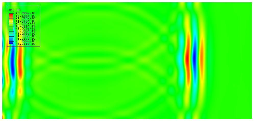
123 (a) x x Figure 5-3: Top view of the wave field at µs. (a) u, (b) u 3. (b) (a) x x Figure 5-4: Top view of the wave field at 4 µs. (a) u, (b) u 3. (b)

124 The wave field distribution in the (x,x 3 ) cross section is shown in Fig. 5-5 when the time is µs. The x direction of the picture starts from the right edge of the loading element. This profile is compared to Fig The numerical result matches the expectation based on normal mode expansion. x 3 x (a) x 3 x (b) Figure 5-5: Thickness profile of the guided wave at µs excited from a mm wide transducer element at khz. (a) u, (b) u 3. Besides the field output, the wave signal at a given point can also be obtained using ABAQUS. To compare the results quantitatively, the results from the theoretical predictions (Fig. 4-3 and Fig. 4-4 ) are plotted together with the results from finite element modeling in Fig. 5-6.

125 3.5 Theoretical prediction FEM calculation u amplitude (nm) x = mm Theoretical prediction FEm calculation -.5 x =4 mm Time (µs) (a). Theoretical prediction FEM calculation u 3 amplitude (nm) x = mm x =4 mm Theoretical prediction FEM calculation Time (µs) (b) Figure 5-6: Wave signal comparison between the theoretical prediction from normal mode expansion and finite element modeling. (a) u, (b) u 3. The black box with dotted line shows the directly excited wave package.

126 4 The black rectangles with dotted lines in Fig. 5-6 indicate the region where the directly excited wave packages arrive at the sensor point. The waveforms after the rectangles in the FEM calculation results are reflected waves and scattered waves. The theoretical predictions match very well with the finite element calculation, quantitatively. This match validates the results from both methods. As a result, the wave excitability defined in Chapter 4 is a good measurement of how efficiently a wave mode can be excited. 5.. Case II: the third wave mode According to Section 4.6.., a shear loading at the edges of a 6 mm wide transducer element can be used to efficiently excite the 3 rd wave mode at khz. The corresponding finite element model was built in ABAQUS with the parameters listed in Tab. 5-. Table 5-:A finite element model parameters to excite the 3 rd wave mode Structure Loading pattern Excitation signal Finite element mesh Lay up sequence [(/45/9/-45) s ] L: Length (mm) 5 W: Width (mm) 7 d: Thickness (mm) 3. Transducer element number We: Element width (mm) 6 Le : Element length(mm) 4 Loading direction Shear traction in x Loading width (mm).5 Loading amplitude (kpa) 3 Center frequency (MHz). Number of cycles 3 Signal window Hanning Mapped mesh with 8 node brick element mesh element size.5mm No. of element per layer

127 5 Fig. 5-7 shows snapshots of the wave field from a top view of the structure, i.e. (x, x ) plane, at µs. The x and x 3 direction displacement is plotted in part (a) and part (b) respectively. The x direction displacement is not shown because the amplitude in the x direction is much smaller than the other components. Since the first mode and third mode are dominated by u 3 and u respectively, the wave field in two displacement components will show different distributions. Figure (a) shows a wave with larger wavelength and group velocity, which is dominated with the third eave mode. Figure (b) shows a wave mode with smaller wavelength and smaller group velocity, which is dominated with the first wave mode. (a) X X Figure 5-7: Wave field snapshots at µs. (a) u field, (b) u 3 field. (b)

128 6 The snapshots of the wave field at µs are shown in Fig The third wave mode has reached the boundaries of the model. Therefore, the reflected waves interfere with the incident wave. Fig. 5-8 (a) shows that the plane wave characteristics of the third wave mode are not preserved very well anymore. However, the first wave mode has a smaller group velocity, it still propagates in its launching direction. The first wave mode can be seen more evidently from Fig. 5-8 (b) since the first wave field is dominant in the x 3 direction. (a) X X Figure 5-8: Wave field snapshots at µs: (a) u field, (b) u 3 field. (b)

129 7 In order to compare the thickness profile of the finite element analysis with the theoretical prediction, the wave field snapshots taken at µs are presented in Fig These results are directly comparable with Fig. 4-3, the only difference is that in Fig. 5-9, the x coordinate is only in the range of [ 95] mm because of the mode size in FEM calculation. (a) x 3 x (b) Figure 5-9: Thickness profile of the guided wave at µs. Comparison of the time domain wave signal is shown for two positions in the model. One is at mm away from the edge of the loading; the other is 4 mm away from the loading. The results of the theoretical prediction and numerical simulation are both plotted in Fig. 5- for comparison purpose. Again, a matching of the wave field validated both methods in the guided wave field analysis.

130 8 u amplitude (nm) x = mm Theoretical prediction FEM calculation x =4 mm Theoretical prediction FEM calculation Time (µs) (a).. Theoretical prediction FEM calculation u 3 amplitude (nm) x = mm Theoretical prediction FEM calculation x =4 mm Time (µs) (b) Figure 5-: Wave signal comparison between the theoretical prediction from normal mode expansion and finite element modeling: (a) u, (b) u 3. Black box with dotted line: excited wave package.

131 Case III: wave modes with large skew angle It was discussed in Section 3.4 that in quasi-isotropic composite laminates, there are some wave modes with large skew angles. Fig. 5- shows the skew angle dispersion curves of the quasi-isotropic laminate for wave propagation in the o direction. The skew angle of the fifth wave mode (high lighted purple line) at.7 MHz has a skew angle of -37 o. In this section, this phenomenon will be validated with finite element simulation in ABAQUS. 4 3 Skew angle (degree) Frequency (MHz) Figure 5-: Skew angle dispersion curve of wave propagation in the o direction of a quasi-isotropic composite laminate. A wave loading pattern is designed to efficiently excite the guided wave mode on the fifth mode line at.7 MHz. The model geometry and loading parameters are listed in Tab The corresponding spectrum of the loading is shown in Fig. 5-. Predicted wave mode components are plotted in Fig. 5-3.

132 Table 5-3: Model geometry and loading pattern to demonstrate large skew angle Structure Loading pattern Excitation signal Finite element mesh Lay up sequence (/45/9/-45)s L: Length (mm) 5 W: Width (mm) 7 d: Thickness (mm) 3. Element Number 5 We: Element width (mm) 3 Le : Element length(mm) 4 Loading direction normal traction in x 3 Loading amplitude (kpa) 3 Center frequency (MHz).7 Number of cycles Signal window Hanning Mapped mesh with 8 node brick element mesh element size.5mm No. of element per layer 8 3 Phase velocity (km/s) Frequency (MHz) Figure 5-: Wave excitation (f-c p ) spectrum for a 5 element transducer with 3 mm element width and excited with a cycled signal at 7 khz using a Hanning window.

133 Figure 5-3: Wave mode content curve for the loading described in Tab The excited wave field at several times are shown in Fig The skew angle of the wave mode can be estimated from the wave field images. The result turns out to be -3 o. The predicted value of the skew angles is from -3 o to -37 o in the frequency range. Therefore, the numerical simulation confirms the prediction of the large skew angle phenomenon in the quasi-isotropic laminate.

134 (a) (b) Figure 5-4: Sample wave field snapshots of u 3. (a).5 µs (b) µs The reason for the large skew angle can be found by using wave structure analyses. Fig. 5-5 shows the displacement profile and the power flow profile of the wave mode (.7 MHz, mode 5). The skew angle effect cannot be directly observed from the displacement wave structure. What can be observed is a strong coupling

135 3 between the displacement in three directions. In the power flow wave structure, it is clear that most of the energy is transmitted in the -45 o layers with layer number 4, 5, and 3. Therefore, this wave mode has a large skew angle with negative value. For the application in SHM, this wave mode will potentially be sensitive for fiber breakage detection and matrix cracking in these plies...5 u P o 45 o 9 o -45 o Displacement u Power flow - P..5 P u Depth (mm) - 3 Depth (mm) Figure 5-5: The displacement and power flow wave structures of the guided wave mode with large skew angle. The mode studied is the fifth wave mode at a frequency of.7 MHz.

136 4 5.3 Summary Finite element simulations were used in this chapter to validate the predictions of the guided wave mechanics theory. Guided wave modes in the quasi-isotropic laminate with different characteristics are demonstrated. As an example, the first guided wave mode at a frequency of khz propagates slower than the third wave mode at the same frequency. The first wave mode at a frequency of khz are excited efficiently with a normal loading on the surface of the laminate. The guided wave mode with large skew angle around -3 degree is also demonstrated. The theoretical predictions made from the normal mode expansion technique match very well with the numerical results obtained in the finite element modeling. The theoretical study using normal mode expansion is computationally more efficient than the three-dimensional finite element method in ABAQUS. The computing times of the models presented in this chapter are about hours in average. However, the normal mode expansion technique only takes several minutes after the dispersion curves are calculated. After the validation with finite element analysis, the normal mode expansion technique can be used for guided wave excitation analysis in composite laminates and elimination the difficulties of trial and error numerical experiments using FEM. Note that, finite element modeling is still useful for wave excitation and scattering analyses in irregularly shaped structures and for wave response from unusually shaped defects.

137 Chapter 6 Guided waves in composites considering viscoelasticity In most ultrasonic wave propagation problems, laminated composites are assumed as elastic. However, at high frequencies, viscoelastic behavior of the material will introduce significant attenuation to the wave propagation. This effect has been neglected in the previous chapters. In this chapter, the influence of viscoelasticity will be addressed for guided wave propagation and excitation in laminated composites. The hybrid SAFE- GMM method developed in Chapter will be used to generate the dispersion curves and the wave structures. The normal mode expansion technique will also be modified to study the wave excitation in lossy composite laminates. 6. Dispersion relation derivation Wave propagation in viscoelastic media can be studied by substituting the elastic constants in the governing equation (Equation. ) with a complex stiffness tensor. The real part corresponds to the energy storage in wave propagation; and the imaginary part corresponds to the damping introduced by the material viscoelasticity [Bartoli et al. 6]. In Equation 6., both C ' and C '' are 6 by 6 matrices. Two models are used in modeling the material viscoelasticity. One is the hysteretic model, where independent. The other is the Kelvin-Voigt model [Rose 999], where function of frequency. The measurement of C' ' is frequency C' ' is a linear C '' at a given frequency f is provided as a 6x6 matrix η. Mathematical expressions for these two models are listed in Equation 6. and Equation 6.3. C = C' ic' ' (6.)

138 6 Hysteretic model: C = C' iη (6.) Kelvin-Voigt model: f C = C' i η (6.3) f When the material properties are substituted into the SAFE formulation, the dispersion curves for the viscoelastic media can be obtained. Different from the wave propagation in an elastic media, the wave numbers obtained from the solution of eigen function Equation.3 are generally complex. The real part is related to the phase velocity of the wave mode; and the imaginary part is related to the attenuation. ω β = ξ + iα = + iα (6.4) c Therefore, two dispersion curves are needed to describe the guided waves in a viscoelastic media. One is the phase velocity dispersion curve, and the other is the attenuation dispersion curve. The wave structure of a particular guided wave mode can be calculated using the hybrid SAFE-GMM method by substituting the complex stiffness constant and complex wave number into the GMM program. The final solution of a guided wave mode can be expressed as Equation 6.5. u( x, x3, t) 3 3) p i( βx ωt ) i( ξx ωt ) αx = U ( x ) e = U ( x e e (6.5) 6. Numerical simulation results on wave propagation Numerical simulations for the quasi-isotropic composite are carried out using material properties listed in Tab. 6-. The real parts of the elastic constants are the same as the ones used in Chapter 3. Due to the limitation in obtaining the imaginary part of the material properties specifically for the IM7/977-3 composite, the properties provided in [Neau et al. ] are used. Although this will not be able to provide exact values of

139 7 attenuation for each guided wave mode, a relative comparison between the guided wave modes can be obtained. The predicted attenuation will also be compared to some preliminary experiment results in Chapter 9. Table 6-: Lamina properties of the IM7/977-3 composite used in simulation Real part (GPa) Imaginary part (GPa) ' C 78 ' C 8.35 ' C ' C 4.4 ' C 3 8. ' C ' C ' C ' C Measurement frequency f '' C 8.3 '' C.65 '' C 3.6 '' C.34 '' C 3.5 '' C '' C 44.4 '' C 55.8 '' C 66.5 MHz Density ρ.6 g/cm 3 Fig. 6- shows the phase velocity dispersion curves and attenuation dispersion curves obtained from the Hysteretic model. In order to show the curves clearly, only those wave modes with attenuation less than neper/mm and phase velocity less than km/s are plotted.

140 8 (a) Figure 6-: (a) Phase velocity dispersion curve and (b) attenuation dispersion curves obtained from Hysteretic model. (b) The relationship between nepers and decibels is expressed in Equation 6.6. neper = log ( e ) db 8.69 db (6.6) = The typical attenuation value shown in Fig. 6- (b) is. neper/mm, which means the wave attenuation is 8.69 db/cm. From this figure, we can also see that the overall trend of attenuation increases with frequency. However, for a specific mode, the attenuation could also decrease with the increase of frequency. In addition, at a specific frequency, we can always find a mode that has the smallest attenuation. As a comparison, the results obtained from the Kelvin-Voigt model are shown in Fig. 6-. Since the reference frequency used in this calculation is MHz, the attenuation for the wave modes at MHz is the same as the values obtained in the Hysteretic model. For the frequencies less than MHz, a smaller imaginary part of the stiffness constant is used according to Equation 6.3, therefore, these attenuation results are smaller than for the Hysteretic model.

141 9 Figure 6-: (a) Phase velocity dispersion curve and (b) attenuation dispersion curves obtained from Kelvin-Voigt model The wave modes having the least attenuation are highlighted in Fig Similar modes are identified in both the Hysteretic model and the Kelvin-Voigt model. Figure 6-3: Wave modes with least attenuation at a given frequency. (a) Hysteretic model (b) Kelvin-Voigt model. Another important issue in the consideration of material viscoelasticity is whether the introduction of material viscoelasticity will affect the phase velocity dispersion curve. In order to answer this question, the dispersion curves obtained from the Hysteretic models and the dispersion curves without considering damping are all plotted in Fig The results indicate that the phase velocity dispersion curve in the elastic model have a

142 good match with the viscoelastic model. This agreement generally validates the usefulness of phase velocity dispersion curves obtained in the elastic model for guided wave applications. Differences occur at mode interaction regions. As is shown in Fig. 6-4 (b), the dispersion curves are two separate lines in the elastic model. However, in the viscoelastic model, the two curves interact with each other. (a) Figure 6-4: Comparison of phase velocity dispersion curves between the elastic model and the Hysteretic viscoelastic model. Dotted line: elastic model, solid line: viscoelastic model. (a) Full set of dispersion curve, (b) Magnified curve shows mode interaction. (b) In the next step, we will compare the wave structures obtained from these two models. As an example, the first wave mode at khz is considered. The x direction displacement distribution obtained from the elastic model and the Hysteretic viscoelastic model is plotted in Fig The result indicates that the difference in the real part of u solution is very slight for these two models. In the elastic model, the imaginary part of u is zero. However, in the viscoelastic model, the u wave structure also has an imaginary part, although its amplitude is only 3% as for that of the real part.

143 (a ) (b) Figure 6-5: Wave structure comparison between the elastic model and the viscoelastic model. Wave mode: first mode at khz, u displacement. (a) real part (b) imaginary part. This tells us that for the wave modes with light attenuation, the wave structure obtained from the elastic model is still a good approximation. For the wave modes with large attenuation, larger differences are observed between the wave structures. With the introduction of attenuation, the definition of guided wave group velocity will be altered. Equation 6.7 repeats the group velocity definition presented in Equation.38. dω c g = dξ ω Q ξ, cg c p c When ξ is complex, the derivative of ξ can not be calculated exactly from the derivative of phase velocity with respect to frequency. However, the energy velocity defined in Equation.4 will still provide a good estimation on the wave energy transmission in viscoelastic media. The comparison between the energy velocity obtained from viscoelastic and elastic models are shown in Fig The comparison shows that the difference only occurs at the mode interaction region. For other modes, the average p c p f dc df p (6.7)

144 difference in energy velocity is below. km/s. Therefore, this information again validates the general accuracy of using an elastic model for guided wave group velocity (energy velocity) prediction. (a ) (b) Figure 6-6: A comparison of energy velocity dispersion curve generated from the elastic and viscoelastic model. (a) elastic model (b) viscoelastic model. One important feature is observed when we compare the energy velocity dispersion curve with the minimum attenuation modes shown in Fig We find that the minimum attenuation modes have strong correlations with the maximum energy velocity modes. We believe this is a new observation and this can be used in future NDE and SHM tests. With this rule, the modes with least attenuation can be selected by only investigating the modes with large group velocity in the elastic model. Fig. 6-7 shows these two sets of curves side by side for a comparison.

145 3 (a) Figure 6-7: Guided wave feature comparisons from a viscoleastic model. (a) Wave modes with largest group velocity for a given frequency (b) Wave modes with smallest attenuation for a given frequency. (b) The comparison between skew angle dispersion curves obtained from the elastic model and the viscoelastic model are presented in Fig The skew angle prediction from the elastic model matches the skew angle from the viscoelastic mode for most of the wave modes. At mode interaction regions, for example the ones indicated with circles, a comparably large difference is observed from the two models. 3 Skew angle (degree) Mode - Mode Mode 3 Mode 4 - Mode 5 Mode Mode -3 Mode 3 Mode 4 Mode Frequency (MHz) Figure 6-8: Comparison of skew angle dispersion curves obtained from elastic and viscoelastic model. Dotted line: elastic model. Solid line: Hysteretic viscoelastic model.

146 4 6.3 A new normal mode expansion technique for viscoelastic media The normal mode expansion technique developed in section 4. is based on the complex reciprocity relation. It is only valid for lossless media. In this chapter, a new normal mode expansion technique for viscoelastic media will be developed. To the knowledge of the author, this is the first attempt to solve this problem. This section will be started with the derivation of wave mode orthogonality in viscoelastic media from the real reciprocity relation shown in Equation 6.8. m n n m n m m n [ v σ v σ ] = v F v F (6.8) First, we will prove mode orthogonality. Assuming m and n are two wave modes with one frequency. The wave mode solutions are in a form of Equation 6.5. For stress free mode solutions, no external force is applied. Therefore both F m and F n are zero. The mode orthogonality equation is in Equation 6.9. Q mn = 4 i( ξ ξ )4Q = m { v n crosssection n mn σ v m m σ } x dx n ˆ 3 (6.9) This means, when β m β (i.e. m n ), n Q = for m n (6.) mn With the wave orthogonality function defined, normal mode expansion can be used to study the wave excitation characteristics. The equation for mode component is expressed in Equation 6.. Q nn ( + iβ n ) a n ( x) = f sn ( x) + f vn ( x ) (6.) x 4 The new f sn and f vn are defined in Equation 6. and Equation 6.3. f sn ( x H ) = { n ( x3) F( x, x3) V( x, x3) σn ( x3)} xˆ 3 y= v (6.)

147 5 Here F is the excitation force and V is the velocity prescription. Solving these equations, the mode expansion coefficients for wave excitation in viscoelastic media are found as in Equation 6.4. Comparing Equation 6.4 with Equation 4., the difference is in the wave mode solutions used to calculate s f and v f. For rightward propagating waves (n>), the wave structure information of the leftward propagating wave (n<) will be used. Both Equation 6.4 with Equation 4. will come to the same solution when an elastic media is considered. This can be proved with the facts listed in Equation 6.5, Equation 6.6, and Equation 6.7. However, for an attenuative wave mode, Equation 6.5 and Equation 6.6 are not valid. 6.4 Numerical simulation results Similar to the case of elastic material, the wave mode excitability from a surface source can be defined as the particle velocity at the surface from a left propagating wave. Since the wave structure solution is generally complex, the absolute value of the particle velocity is a good measurement of the excitabilities. Three excitability curves can be = H n vn dx x x x x f ), ( ) ( ) ( F v (6.3) ) ( ) ( ) ( ) ( ) ( ) (, ) exp( 4 ) ( ) ( ) exp( ) (, ) exp( 4 ) ( ) ( ) exp( ) (, ) ( x L d i Q f f x i x a L x L d i Q f f x i x a L x x a L L n n n n v n s n n x L n n n n v n s n n n < + = + = = η η β η η β η η β η η β (6.4) ) ( ) ( 3 3 * x v x v n n = (6.5) n ξ n β = (6.6) nn n n P Q = ) ( (6.7)

148 6 defined for the loading in x, x and x 3 directions respectively. As an example, Fig. 6-9 shows the wave excitability of the first three wave modes using loading in the x direction. The corresponding excitability in the elastic model is also shown as a comparison and is represented by the dotted line. Differences are observed in the mode conversion region and the higher attenuative region..5.. Excitability F.5..5 Excitability F Frequency (MHz) (a ) (b) Frequency (MHz) Figure 6-9: Comparison of wave mode excitability with x direction force on the surface. Dotted line: Elastic model; solid line: Viscoelastic Hysteretic mdoel. (a) Frequency range of to MHz. (b) Magnified region of mode interaction. Mode components from a finite source can be obtained from Equation 6.4. Fig. 6- show the wave mode excitation performance using a 4 mm wide element of x direction shear loading. The amplitude of the load is N. The result shows that at low frequency, the wave excitabilities are almost not changed. However, for high frequency and severe damped modes, the wave mode excitability is reduced in the viscoelastic model.

149 7 Excitability x Excitability x Frequency (MHz) (a).5.5 Frequency (MHz) Figure 6-: A comparison of wave mode excitability using F direction loading in (a) an elastic and (b) a viscoelastic model. (b) 6.5 Summary Material viscoelasticity of a laminated composite is considered in this chapter. Several conclusions and observations of wave propagation and excitation are summarized as follows.. With an introduction of material viscoelasticity, an attenuation dispersion curve can be obtained for guided wave modes. The attenuation dispersion curve provides a guideline for estimating the propagation distance of a wave mode.. From the attenuation dispersion curve, the wave modes with least attenuation are studied. The results of the least attenuative modes match with the wave modes with maximum group velocity. 3. Introducing a weak attenuation does not significantly affect the phase velocity, group velocity, skew angle and wave structure of a guided wave mode. Therefore, most of the results obtained from an approximated elastic model are still valid. However, the introduction of

150 8 attenuation affects the mode interaction and dispersion curve crossing. At these local regions, the dispersion curves will be modified. 4. The introduction of attenuation into the modeling affects the procedure of normal mode expansion. A new normal mode expansion formula is derived in this thesis starting from the real reciprocity relation. With this formula, the wave excitation characteristics in a viscoelastic composite can be studied. The result shows that the introduction of attenuation affects the wave mode coefficients and the excited wave field.

151 9 Chapter 7 Guided wave sensitivity to damage in composites Two types of damage could occur in engineering composites from a guided wave modeling point of view. One is introduced by long term environmental aging and fatigue. The distributed microscopic fiber breaking and matrix cracking can be modeled as global material property degradation. Detection of global material property change with guided waves could provide early warnings to more severe damage types. Another type of damage is modeled in such a way that a delamination or damage introduced by mechanical impact appears as a discontinuity in material properties. In this case, wave scattering phenomenon could be used to detect the damage. Influences of these two types of modeled damages on guided wave propagation are studied in Section 7. and Section 7. respectively. 7. Effect of material property degradation on guided wave propagation 7.. Theoretical study Density, stiffness constants, and thickness of the layers are key material properties affecting guided wave propagation. Equation 7. is the governing equation for wave mode analysis in the semi-analytical finite element formulation. [ ξ K + i ξ ( K K ) + K ω M] U = (7.) Details for M, K, K, K, and K are listed in Equation.6. Assuming the density of the material changes by a factor ( a ), the influence on phase velocity dispersion curve is derived in Equation 7..

152 3 ρ = aρ => M = am when ξ = ξ, => ω = ω, f = f, a a c p = c p (7.) a Therefore, the phase velocity dispersion curve expands and shrinks proportionally with respect to ( f, ) = (,). When the density increases, the dispersion curve shrinks; when c p the mass density decreases, the dispersion curve expands. Similarly, if the elements in the stiffness constant matrix all change together with a factor (b), the changes in dispersion curves are derived in Equation 7.3 C = b => K ) = b( K ), m, n =, C ( mn mn when ξ = ξ, => ω = bω, f = b f, c = bc (7.3) p p Therefore, the phase velocity dispersion curve also expands with increased stiffness and shrinks with reduced stiffness. When the elements of the stiffness constant do not change together, the changes in guided wave dispersion relation will be more complicated. Numerical simulation is needed to predict the dispersion curve at degraded states. 7.. Density variation The relation of the phase velocity dispersion curve to the density is now studied numerically as a proof to the derivation of Section 7... The results presented in this section are for the wave propagation in the o direction of a quasi-isotropic laminate. The nominal density is.6 kg/m 3. Fig. 7- plotted the dispersion curves for the undamaged material (blue) and the material with % density reduction (red). This figure confirms that with the reduction of density, the dispersion curves expanded in both f and c p axis. The variation of mass density affects the velocity of each mode as well as the cut-off frequency of the mode lines.

153 3 Phase velocity (km/s) Blue: Original Red: % reduction.5.5 Frequency (mm) Figure 7-: Dispersion curves for guided wave propagation in composite laminates. Blue dashed line: nominated mass density of IM7/977-3 ρ=.6 kg/m 3 Red line :assumed % density reduction ρ=.44 kg/m Elastic stiffness variation As was predicted in Section 7.., when all components of the elastic stiffness vary at the same rate, the dispersion curve corresponding to the degraded structure can be predicted from the pristine structure using Equation 7.3. Fig. 7- confirms this rule with a structure whose stiffness matrices are reduced % from the nominal elastic stiffness constants. The blue dashed lines are the dispersion curves for the structure without stiffness reduction. The blue solid lines are the predicted dispersion curve for the stiffness reduced structure from proportional scaling. The red dots are the representative points calculated with a stiffness-reduced model. A good match is observed between the blue solid lines and the red dots.

154 3 Phase velocity (km/s) Frequency (mm) Figure 7-: Figure illustrates the effect of dispersion curve scaling when the material property degradation introduces % stiffness reduction. Blue dashed line: no stiffness reduction, blue solid line predicted dispersion curve with stiffness reduction, red dots calculated dispersion curve with stiffness reduction. In real situations, the components of the elastic stiffness matrix do not necessarily vary together. Therefore, studying the effect of changing a particular engineering constant is valuable for both damage detection and material property estimation. Comparison of % change of E, E, G, ν, and ν 3 on the dispersion curves are shown in Fig. 7-3 through Fig These figures indicate that the variation of E significantly affects the phase velocity dispersion curves of u dominant wave modes in the c p axis. Therefore, the second and the third fundamental modes can be used to detect this change efficiently. Degradation of E shifts the u 3 dominant wave modes in the frequency axis. The second and third wave modes around.4 MHz could be sensitive modes to detect this change. Changing G affects the cut off frequency of most of the modes especially the u dominant wave modes. A broadband excitation and frequency domain analysis would be

155 33 a benefit in detecting this change. Poisson s ratio v only has slight effects on the dispersion curves. Therefore its values are not very critical in dispersion curve generation. Poisson s ratio v 3 affects the dispersion curve of some higher order wave modes at high frequency. Phase velocity (km/s) Frequency (mm) Figure 7-3: Effect of engineering constant variation on guided wave dispersion curves. Blue dashed line: nominated material property. Red line: with % fiber direction modulus (E ) reduction of the lamina.

156 34 Phase velocity (km/s) Frequency (mm) Figure 7-4: Effect of engineering constant variation on guided wave dispersion curves. Blue dashed line: nominated material property. Red line: with % transverse modulus (E ) reduction of the lamina. 8 6 Phase velocity (km/s) Frequency (mm) Figure 7-5: Effect of engineering constant variation on guided wave dispersion curves. Blue dashed line: nominated material property. Red line with % in plane shear modulus (G ) reduction of the lamina.

157 Phase velocity (km/s) Frequency (mm) Figure 7-6: Effect of engineering constant variation on guided wave dispersion curves. Blue dashed line: nominated material property. Red line with % Poisson s ratio(v ) reduction of the lamina. Phase velocity (km/s) Frequency (mm) Figure 7-7: Effect of engineering constant variation on guided wave dispersion curves. Blue dashed line: nominated material property. Red line with % Poisson s ratio (v 3 ) reduction of the lamina.

158 Ply thickness variation It is commonly recognized in the use of guided waves in single layer isotropic material that the frequency thickness product is a characteristic quantity in both the phase velocity and group velocity dispersion curves. However, frequency is used as a variable throughout this thesis. This is because in a multilayered structure the thickness of each layer has an effect on the dispersion relation of the structure. The variation of the total thickness can not uniquely define the behavior of the structure. In laminated composites, the effect of the variation in the thickness of the prepreg on the dispersion curves is shown in Fig.7-8. Dispersion curves for two 6 layer structures with. mm and.8 mm ply thickness are plotted with blue curves and red curves respectively. The result indicates that the curves are scaled in the frequency axis only. The most significant effect of the ply thickness change on the dispersion curve is the shifting of cut off frequencies. Phase velocity (km/s) Frequency (mm) Figure 7-8: Variation of dispersion curves due to ply thickness change of a 6 layer quasi-isotropic composite. Blue lines:.mm Red lines:.8mm.

159 37 A common damage to the composite material is surface erosion. The effect of the first ply thickness reduction on guided wave dispersion curves are illustrated in Fig. 7-9 In this figure the blue lines are for the structure with ply thickness. mm. The red lines are for the structure with the first ply thickness reduced to. mm. In this case we could see that the most significant change in the dispersion curve is the shifting of the cut off frequencies of the higher order modes. Phase velocity (km/s) Frequency (mm) Figure 7-9: Effect of surface erosion on guided wave phase velocity dispersion of a 6 layer quasi-isotropic composite laminate. Blue line: all ply thickness. mm. Red line: first layer thickness reduction of. mm. 7. Guided wave scattering sensitivity Wave scattering is an important issue in damage detection using ultrasonic guided waves. The existence of a flaw in a material is usually detected from its echo signal. However, quantitative analysis of guided wave scattering in composite material is very

160 difficult. Although finite element analysis can be used to calculate wave scattering for a given situation, the extrapolating of the results to a different case is difficult. In this section, we put forward a hypothesis on guided wave scattering sensitivity to damage in composites based on an analytical wave scattering study. 38 In [Auld 99], an S-parameter method is used as an indication of how much energy of the incident wave is converted into reflected waves and mode-converted transmission waves. Numerical expression of the S parameter is in Equation 7.4 Here, S F is the surface of the damage, nˆ is the direction normal at the surface of the damage. The wave field in the undamaged state and the damaged state are denoted with ' ( v, σ ) and ( v and ' σ ) respectively. When we want to study the wave mode scattering sensitivity, the wave field of the undamaged state is the incident wave mode. In the case of a delamination, the damaged wave field can be approximated as stress free at the debonded surfaces ( σ '= ). Therefore, Equation 7.5 describes the wave scattering parameter in the case of delamination. ' ' S = nds Ml Nr ( v σ v σ) ˆ, (7.4) 4 S F ' S = nds Ml Nr ( v σ) ˆ, (7.5) 4 Equation 7.5 indicates that the wave mode conversion parameter is related to the stress distribution of the undamaged field, the wave velocity of the damaged field at the delamination boundary, and the shape of the delamination. The shape of the delamination is case dependent, and the wave field at the delamination boundary after delamination occurred is difficult to obtain. However, from the equation, it is quite clear that the sensitivity of a guided wave mode to detect a delamination is directly related to the stress distribution (σ ) of the incident wave mode at the position of the delamination. S F In the case of a delamination, the surface normal nˆ is in the x3 direction. Therefore, the following hypothesis is put forward to estimate the sensitivity of a guided wave mode for delamination without considering the detailed size of the delamination.

161 39 To maximize the sensitivity of a guided wave to a delamination at a certain depth, the stress components normal to the (x, x )plane ( σ 33, σ 3, σ 3) should be maximized. Therefore, one sensitivity metric can be formulated as in Equation 7.6. Sensitivit y = σ + (7.6) 33 + σ 3 σ 3 As an example, when the structure is a [(/45/9/-45) s ] laminate, the sensitivity spectrum of the first six wave mode lines for the wave propagating in the o direction are shown in Fig. 7- to Fig. 7-. In these two cases the delamination is located at the first interface (between o and 45 o ) and the third interface (between 9 o and -45 o ) Mode Mode Mode 3 Mode 4 Mode 5 Sensitivity Frequency (MHz) Figure 7-: Estimated sensitivity spectrum of guided wave modes to delamination at the first laminate interface of a [(/45/9/-45) s ] composite structure.

162 4 3.5 Mode Mode Mode 3 Mode 4 Mode 5 Sensitivity Frequency (MHz) Figure 7-: Estimated sensitivity spectrum of guided wave modes to delamination at the 3rd laminate interface of a [(/45/9/-45) s ] composite structure. In most cases, the location of the delamination can not be precisely predicted in structural health monitoring. Therefore, a general evaluation of the sensitivity to delamination in an arbitrary layer would be helpful. In order to do this, a general sensitivity definition is presented in Equation 7.7. Here, N is the total number of layers. N- is the number of interfaces. Sensitivity = N ( Interfaces σ 33 + σ 3 N + σ 3 ) (7.7) Fig. 7- is the overall sensitivity estimation of guided waves in the 6 layer quasi-isotropic laminate.

163 Mode Mode Mode 3 Mode 4 Mode 5 Sensitivity Frequency (MHz) Figure 7-: Estimated sensitivity spectrum of guided wave modes to delamination in a [(/45/9/-45) s ] composite structure. 7.3 Summary In this chapter, influences of damage on guided wave propagation characteristics are studied. Long term aging is modeled with a change of composite density, stiffness constant, and thickness variation. The results on guided wave propagation are summarized as follows.. When the density of a composite decreases by a factor of a, the phase velocity dispersion curve expands in both frequency and phase velocity axes by a factor / a.. When the stiffness of the composite material decreases by a factor of b, the phase velocity dispersion curve shrinks in both frequency and phase velocity axes by a factor of b. 3. Studies of influence of each engineering constant change on guided wave dispersion curves are also performed. Decreasing E shrinks the

164 4 dispersion curve on the phase velocity axis. The effect is particularly significant for u dominant wave modes. Decreasing E shrinks the dispersion curve in the frequency axis. The phenomenon is significant for quasi R-L type wave modes, especially for u 3 dominate modes. Decreasing G shrinks the dispersion curve in frequency axes. The phenomenon is significant for quasi shear horizontal waves. Influence of Poison s ratio on dispersion curve is not very significant, especially at lower frequency. 4. When the thickness of each lamina decreases by a factor of a, the dispersion curve expands in the frequency axis by a factor of a. The surface erosion in a composite also affects the dispersion topology by expanding slightly in the frequency axes and the reduction of phase velocity at low frequency. Although the details of the material degradation are not explored in this thesis study, the rules obtained in this section will be important for selecting a good mode to detect material degradation. In addition, these rules can also be used in material property characterization. By detecting the changes in dispersion curves, mistakes in lay-up sequence could also be detected. In Section, the expected sensitivity of a guided wave mode to localized damages is studied. The formulation of the sensitivity is based on an analytical study of guided wave scattering. A new sensitivity definition for guided wave mode selection is proposed using stresses at the damage surface. Specific results are provided for delamination detection. They indicate that commonly used fundamental wave modes 3 at low frequency are not sensitive to delamination.

165 Chapter 8 Guided wave mode selection 8. Introduction In the previous chapters, many features related to a guided wave mode in composite materials have been obtained. Chapter 3 studied the phase velocity, group velocity, and skew angle of a wave mode when the material was assumed elastic. Chapter 4 studied the wave excitation, dispersion, and beam spreading characteristics. Chapter 6 evaluated the viscoelastic effect on the wave propagation and excitation. In addition to all the features studied in Chapter 3 and Chapter 4, the attenuation characteristic of a guided wave mode is introduced. Chapter 7 studied the expected wave mode sensitivity to different kinds of structural damage especially delamination in composites. How to comprehensively evaluate all these features and select the most suitable wave mode candidates for an inspection task becomes the next problem to address. A wave mode might have superior performance in terms of one feature but it is not very good in terms of another feature. For example, mode 3 at low frequency has the least attenuation; therefore it is a candidate for long range inspection. However, its sensitivity to delamination is not good compared with other modes. There are also two ways of evaluating a feature. One is a crisp selection method. For example, when the wave mode skew angle is less than degrees, it is acceptable. When it is larger than degrees, it will not be selected. Another evaluation method is based on fuzzy analysis. As an example, when one says a wave propagates fast, we are not referring to the group velocity larger than a specific value to be fast and below that to be slow. We are thinking in a way that the larger the value is, the faster it is. In order to have a flexible and comprehensive evaluation of the guided wave mode features, a set of mode selection rules will be used.

166 44 8. Guided wave mode selection rules A mode selection rule is a descriptive criterion that states how a guided wave feature will satisfy our inspection goal. Two types of rules are considered. One is a crisp mode selection rule, which means the mode either satisfies the condition or not. The other is a fuzzy mode selection rule. For both of these cases, a goodness function will be used to describe how a mode qualifies the requirements. As an example, we can select those wave modes with an attenuation rate below.5 db/mm to be qualified wave modes for long range monitoring. For this case the goodness function of attenuation is shown in Fig. 8- (a). In a fuzzy case, a wave mode with an attenuation rate below. db/mm will be considered perfect, and the ones above db/mm will not be acceptable and the goodness ramps in between. (a) Figure 8-: Goodness function definition for guided wave selection. Evaluates attenuation characteristic (a) Crisp rule (b) fuzzy rule. (b) The corresponding mode selection results for the guided wave propagating in the o direction of the [(/45/9/-45) s ] laminate is shown in Fig. 8-. The attenuation dispersion curve from the Hysteretic model described is used. The mode selection result is superimposed on the phase velocity dispersion curves. In Fig. 8- (a), the wave modes that meet the criterion are plotted in red. In Fig. 8- (b), the mode goodness results are plotted in color with red as one and blue as zero. Basically, the results indicated that

167 guided waves at a low frequency are good. If the desired frequency is higher, only some specific modes can satisfy the requirement. 45 (a) (b) Figure 8-: Mode selection results considering wave mode attenuation. (a) Crisp mode selection with.5db/mm allowed. (b) Fuzzy selection. Enlightened from the filter design concepts in electrical engineering, our goodness function can also be defined as low path, high path, band path, or band stop distributions. As an example, if we want to illustrate the possibility of large skew angle wave modes in a quasi-isotropic composite laminate. We will select those modes with large skew angles. The rule and the corresponding mode selection results are shown in Fig. 8-3.

168 46 (a) Figure 8-3: The mode selection rule and candidate wave modes for large skew angle demonstration. (a) High pass filter for the absolute value of skew angle. (b) Mode selection results. (b) The mode selection with a single criterion has been discussed. However, in a practical design, many parameters need to be considered to make a decision. The joint consideration of a group of mode selection criteria can be carried out in the following steps.. Any wave mode that does not satisfy the crisp rules will be excluded from the pool of candidates.. The fuzzy rules can be evaluated in two ways. (a) Average the fuzzy rules with specified weights for each rule. (b) Choose the minimum value of goodness from all the rules to be the final goodness value. This will keep those wave modes with good performance for all the rules. 3. Combine crisp and fuzzy rules. For example, in order to show the wave modes with large skew angle, the modes with excessive attenuation will be excluded. If we apply the rules described in Fig. 8-3 (a) and Fig. 8- (a), the results are shown in Fig The fifth wave mode around.69 MHz and 5. km/s phase velocity will be a good mode to show the concept.

169 47 Selected mode Figure 8-4: Guided wave mode selection for the purpose of demonstration large skew angle. 8.3 Guided wave long range monitoring potential In structural health monitoring, long range wave propagation potential will be explored. In order for the waves to propagate long distances, the wave attenuation rate and wave dispersion coefficient should be small; the wave excitability should be large. In addition, for appropriate damage detection, the expected sensitivity should be large. Whether the selected wave mode could be suitable for a practical transducer design is also an important issue. Here, we will focus on selecting the guided wave modes with desired performance. First, we will study the mode selection for each criterion. Tab. 8- lists some rules to be considered in the design.

170 Table 8-: Proposed mode selection rules for mode selection based on long range delamination detection in composite laminates. Rule No Feature Rule Attenuation Fuzzy Rule: Low pass [..5] db/mm Dispersion Fuzzy Rule: Low pass [..3 ] µs/mm 3 Sensitivity Fuzzy Rule: High pass [..5] 4 Excitability F Crisp Rule: High pass.5 5 Excitability F3 Crisp Rule: High pass. 48 The mode selection performance for each individual rule is studied as follows from Fig. 8-5 to Fig (a) Figure 8-5: Guided wave mode selection considering attenuation. (a) selection rule (b) selection result. (b) Figure 8-5 is a representation of wave mode attenuation characteristics. The result indicates that wave modes in the low frequency region can propagate a long distance. Figure 8-6 selected the less dispersive wave modes. Figure 8-7 selected the wave modes with reasonable sensitivity to delamination. It shows that the low frequency regions of the second and third wave mode are excluded. Figure 8-8 and Fig. 8-9 shows the wave mode selection with reasonable excitation performance using x and x 3 direction loading respectively. Since in the composite plate the guided wave modes generally have displacement components in all three directions, traditional Lamb modes and SH modes

171 49 cannot be strictly identified. Using x and x 3 directional loading basically generates those wave modes with dominant response in x and x 3 plane. These wave modes can be recognized as quasi-lamb mode. We also see that the third mode at low frequency can be efficiently excited with an x directional loading but not with a loading in the x 3 direction. (a) Figure 8-6: Guided wave mode selection considering mode dispersion. Less dispersive modes selected (a) selection rule (b) selection results. (b) Figure 8-7: Guided wave mode selection considering mode sensitivity (a) selection rule (b) selection result.

172 5 (a) Figure 8-8: Guided wave mode selection considering wave excitation with loading in the x direction. (a) Selection rule (b) qualified wave modes plotted in red. (b) (a) Figure 8-9: Guided wave mode selection considering wave excitation with loading in the x 3 direction. (a) Selection rule (b) qualified wave modes plotted in red. (b) In order to select a mode that can efficiently detect delamination in a composite plate with long range coverage, a comprehensive mode selection will be performed to evaluate the features expressed above. When we set the weight of importance for rule,, and 3 to be.6,., and., and an x direction loading (rule 4) is considered, the overall goodness of the wave modes are plotted in Fig. 8-. The result indicates that the low frequency region of mode and 3 are the best choice. However, because of the trade-off in attenuation and sensitivity, none of the wave modes has absolute preference. In addition, the mode 5 and 6 around 5 khz to 9 khz is also valuable to be explored.

173 Other regions of the dispersion curve will produce either less propagation distance or reduced sensitivity Figure 8-: Overall guided wave mode selection considering rules to 4 listed in Tab. 8-. The results of mode selection provided some general guidelines for guided wave mode selection. It direct us to the parts of dispersion curves that are most likely going to produce good testing results. A detailed wave excitation and propagation analysis can be performed using the simulation tool expressed in Chapter 4. A detailed wave scattering analysis can also be performed with numerical simulations, such as finite element analysis.

174 Chapter 9 Experimental studies In this chapter, some experiments on guided wave mechanics in composite materials are presented to validate the observations in the theoretical study. The composite material is fabricated from unidirectional composite prepreg purchased from Cytec Engineered Materials. The laminate was constructed by hand lay up at the Composite Manufacturing Technology Center (CMTC) and cured in an autoclave in the Applied Research Lab at Penn State University. Detailed documentation of our composite preparation process can be seen in [Bell 4; Noga 6]. In section 9., guided wave phase velocity dispersion curves, wave attenuation characteristics, and skew angle effects are studied. Section 9. studies the wave excitation in composites using surface mounted piezoelectric transducers. Section 9.3 presented some preliminary studies on guided wave damage detection. Comparisons are made between guided wave modes and different transducers. 9. Wave propagation study with contact transducers 9.. Ultrasonic transducers and instruments Fig. 9- shows two test setups to excite ultrasonic guided waves in a 6 by 6 composite plate. The waves are generated using piezoelectric transducers on the left side. A transducer can be put directly on the plate or through a variable angle wedge. The two test methods are called normal incidence and oblique incidence, respectively. The transducer on the right side is used to pick up the ultrasound signal.

175 53 Oblique incidence Normal incidence Transmitter Receiver Figure 9-: Test setups for ultrasonic guided wave propagation study. Fig. 9- shows an integrated ultrasonic testing system. Excitation signals are sent out from the system to the transmitter. The system is also used for data acquisition and preliminary signal processing. Figure 9-: Integrated ultrasonic testing system.

176 Experimental phase velocity dispersion curve Firstly, we will study the wave propagation along the zero degree direction. A pair of khz transducers is used in normal incidence. The excitation signal is a micro second pulse with khz center frequency. When the transmitter is located mm from the left edge of the plate, and the receiver is at mm, the ultrasonic guided wave signal is shown Fig The guided wave signal is complicated in the sense that multi wave packages and multi-modes exist. In addition, multiple reflections from the edges of the plate are also collected in the signal. 5 5 Amplitude Time (µs) Figure 9-3: Guided wave signal collected at mm position, when the transmitter is at from the left edge. A theoretical phase velocity dispersion curve is shown in Fig. 9-4 with the guided wave mode lines named in a numerical order. Despite the complexities of the guided wave signal shown in Fig. 9-3, each wave package within the signal can be designated with guided wave mode analysis. One method to identify the wave package is to keep track of the wave propagation by scanning the receiver along the wave path. A series of guided wave signals are shown in Fig. 9-5 (a). From this figure, we can observe

177 55 multimode propagation, wave reflection, and interference. The first few wave packages are marked in Fig. 9-5 (a), with the wave paths shown in Fig. 9-5 (b). The wave package marked with red arrow and number is the direct excited mode 3, the wave package marked with red arrow and number is the mode 3 sending out to the left and then reflected from the left edge and propagating to the right. The wave package marked with red arrow and number 3 is the left propagation wave reflected from the right edge of the plate. We also notice that, there is a wave package propagating in a much lower velocity. This is the mode marked with the blue arrow and number 4. There are also other reflections occurred in later time Cp (km/s) Frequency (MHz) Figure 9-4: Ultrasonic guided wave phase velocity dispersion curve for wave propagating in the o of a quasi-isotropic composite laminate. Wave mode lines are numbered on the dispersion curves.

178 56 Position (mm) Time (µs) (a) Signals 4 3 Transmitter Receiver (b) Sketch Figure 9-5: Guided wave signals collected from a linear scan showing edge multi-mode, edge reflection, and complex interference. (a) Experimental signals. (b) sketch of the first few wave paths. (): direct transmission mode 3, () Reflected mode three from left edge, (3) reflected mode 3 from right edge, (4) direct through transmission of mode.

179 57 The phase velocity of a mode can be obtained by tracking the waves with a constant phase angle. The estimated value from experiments are 6.45 mm/µs and.48 mm/µs for mode 3 and mode respectively. The expected values from numerical simulation are 6.6 mm/µs and.5 mm/µs. Therefore, the error between numerical simulation and experiment is.5% and.3% respectively. Besides time domain signal analysis, the ultrasonic signal can also be evaluated in frequency domain. A two dimensional Fourier transform can be used to convert the time and spatial domain information into frequency and phase velocity space. A D FFT of the signal is shown in Fig Although the signals are complicated in time domain, they are easy to analyze in the transformed domain with guided wave theory. Besides the wave modes consisting most of the energy, some content of higher frequency waves are also revealed. One drawback of the D FFT is the resolution of wavelength is limited by the step of the linear scan. The step size used in the scan is 5mm. The wave length of the mode at khz is about 7.5 mm, which is below the resolvable wavelength Cp (km/s) Frequency (MHz) Figure 9-6: Frequency and phase velocity spectrum of guided wave signals shown in Fig. 9-5.

180 58 In order to explore the guided wave propagation possibilities, another four pairs of transducers with center frequency at 5kHz, 8kHz, MHz, and a broad band transducer covering khz to 7kHz are used in normal mode incidence test. In addition, the broad band transducer pair is also used with a variable angle wedge at o, 5 o, 3 o, 45 o, and 6 o incident angles. A combined (f-c p ) spectrum obtained from all the tests after data fusion is shown in Fig The theoretical dispersion curve of the wave propagating in the o direction is also superimposed in the figure for the purpose of comparison. A good match between the theory and the experiment is obtained. The match between the experiment and the theory basically proved two things. One is the credibility of the theoretical simulation tool. The other is the material property used in the simulation is close to the actual material property value Cp (km/s) Frequency (MHz).3.. Figure 9-7: A comparison between the experimental dispersion curve and theoretical dispersion curve for wave propagation along the degree direction. The influence of spatial domain sampling rate on the experimental dispersion curve generation is also manifested in Fig The wave modes with high frequency

181 and low phase velocity, i.e., small wavelength, are not represented in the experimental dispersion curve. 59 The experimental dispersion curve shown in Fig. 9-7 is only a subset of the theoretical dispersions. Wave dispersion, attenuation, skew, and the source influence can be used to explain this phenomenon. The strong regions in the experimental dispersion curve are related to the wave modes with easy excitation with normal loading, small attenuation, and small skew angle. If we select the guided wave modes with attenuation less than.5db/mm, skew angle within than.5, ±, and excitability with normal loading larger using the comprehensive mode selection algorithm, the remaining wave modes are plotted in Fig. 9-8 together with the experimental dispersion curves. The wave modes qualified with these rules matched very well with the experiment result. Experimental curve breaks at two frequencies are also investigated. The reason for this is the source influence, because our excitation signal is a 6 micro second tone burst with 5kHz center frequency for the broad band transducer. The frequency spectrum have zeros at.33mhz and.66 MHz.

182 Cp (km/s) Frequency (MHz) Figure 9-8: Comparison of guided wave modes in the experiment with theoretical expectation using low attenuation, low skew angle, and excitable rules, and frequency spectrum of source influence. The result shows that the experiment total meets the expectation Guided wave group velocity and attenuation study Group velocity and attenuation of a guided wave mode can also be extracted from guided wave linear scan experiments. Fig. 9-9 shows the guided wave signals for the mode 8 in the frequency range of.7mhz to.8 MHz. The transmitter is located at mm position, and receivers are at a series of positions from 5mm to 35 mm. A significant difference between the phase velocity and wave package velocity can be noticed from the signals. An estimation of these two velocities can be obtained from the slopes of line and line in the figure. The results are 9.5 km/s and 4.9km/s for phase velocity and group velocity respectively. The range of theoretical prediction are [9.6.6] km/s for phase velocity and [5. 5.4] km/s for group velocity respectively. The slight discrepancy between theory and experiment might be attributed to the inexact

183 material property used in the simulation and also measurement accuracy in the experiment Position (mm) 5 3 Cp (km/s) Time (µs) (a).5.5 Frequency (MHz) Figure 9-9: Guided wave signals from a 8kHz transducer. (a) Illustration of guided wave phase velocity and group velocity in a wave package. (b) frequency and phase velocity spectrum (b) Attenuation information can also be observed from Fig Wave mode attenuation can be estimated with energy reduction of the wave package. Fig. 9- shows the energy content in the signals as a function of position. The linear fitting of the data in log scale suggests the attenuation rate of this guided wave mode to be. db/mm.

184 6 Relative Amplitude (db) y = -.*x + 5 Relative Energy linear fitting Position (mm) Figure 9-: Energy content in the guided wave signal as a function of position showing wave attenuation. Tab. 9- listed the results of estimated attenuation of other guided wave modes from both experimental tests and the predictions from both the Hysteretic model and the Kelvin-Voigt model. Table 9-: Quntitative comparison of wave mode attenuation Wave mode Attenuation (db/mm) Frequency (khz) Mode Number Measurement Hysteretic model K-V model The result shows that although the imaginary part of the complex stiffness value used in the simulation is not exact, the attenuation prediction is in an acceptable scale. The experiment result generally lies in between the attenuation result estimated from the two models. At low frequency the hysteretic model is more close to experiment; at higher

185 63 frequency the K-V model are closer. Quantitative analysis of attenuation will be studied in the future after the viscoelastic material properties for this material are determined Guided wave skew angle study Guided wave modes with large skew angles have been predicted in the theoretical study and validated in finite element analysis. In this section, an experiment is carried out to validate the skew angle in composite plates. The experimental setup is shown in Fig. 9-. A pair of angle wedge transducer is used to transmit and receive waves. The wave vector direction is kept in degree, i.e., the direction parallel to fiber direction of the first layer. The receiving wedge is also kept in the degree direction. The receiver is then moved along the vertically line mm away from the transmitter. y mm Transmitter Wave vector direction x Receiver Figure 9-: Experiments to test the effect of energy skew in a quasi-isotropic composite plate. Based on the mode selection results presented in chapter 8., the fifth wave mode around 69kHz is used. The receiving signals at a series of positions are plotted in Fig. 9-. Strong signals are received below the centerline, with a maximum at the 6mm position. Since the separation of transducers in x direction is mm. The skew

186 angle is estimated to be -3 degree. This result validated the prediction value of degree Position (mm) Time (µs) Figure 9-: Guided waves excited from angle wedge to validate the concept the concept of large skew angel. The black line at the center corresponds to the wave launching direction. The line in -6 mm position marks the position where a maximum signal is detected.

187 65 9. Wave excitation with piezoelectric active sensors The theoretical study indicated that source influences are very important in wave excitation. Influence of piezoelectric element geometry on wave excitation is studied in this section. The elements used are all 4mm long with widths of 4mm, 6mm, and 8mm. These elements are attached on the composite in three groups with mm spacing between the transmitters and the receivers. The piezoelectric material used in the study is CTS 33HD. Fig. 9-3 shows the received signals from these three pairs of transducers. The excitation signal is a khz tone burst with 5 µs pulse width. The wave package arriving at around 4 µs is the direct through transmission signal of mode 3. The wave package arriving about 4 µs is the direct through transmission signal of mode. Other wave packages in between are the reflections from the edge of the plate. Durations of the wave packages shown in the signals are typically longer than the excitation pulse width. The ringing of the transducer element after excitation is the major reason for this. Wave dispersion also contributes to this effect. Although quantitative analysis of the signal still needs more investigation on the transmitter and the receiver responses, the effect of the source influence on wave excitation is already demonstrated in the signals. The relative amplitude between the direct through transmission mode 3 and mode amplitudes changes with the change of element width. When the element width is 4mm and 6mm, the amplitudes of mode are larger than the amplitudes of mode 3. However, when the element is 8mm, the amplitude of the mode 3 becomes dominant. This phenomenon can be explained with the wave mode decomposition spectra. In Fig. 9-4, plots (a), (c), and (e) are for the cases of evenly distributed normal loading; plots (b), (d), and (f) are for the case of concentrated shear loading at the edge of the transducer element. Plots (a) and (b) are for the 4mm transducer element; plots (c) and (d) are for the 6mm transducer element; plots (e) and (f) are for the case of 8 mm transducer element. In both normal loading and concentrated shear loading cases, the amplitude of mode reduces with the increase of element width; while the amplitude of mode 3 increases with the increase of element width.

188 66 Amplitude Mode 3 Mode 5 5 Time (µs) (a) Amplitude Time (µs) (b) Amplitude Time (µs) (c) Figure 9-3: Guided wave signals from surface mounted piezoelectric transducers. Excitation signal khz, pulse width 5 µs. transducer element width (a) 4mm, (b) 6mm, and (c) 8mm.

189 Mode.5. Excitability Excitability.5. Mode Mode 3.. Mode Frequency (MHz) Frequency (MHz) (a ) 4mm transducer normal loading (b) 4mm transducer shear loading Mode. Excitability Excitability.5. Mode Mode 3. Mode Frequency (MHz) (c) 6mm transducer normal loading Frequency (MHz) (d) 6mm transducer shearl loading Mode. Mode 3 Excitability Mode 3 Excitability.5. Mode Frequency (MHz) (e) 8mm transducer normal loading Frequency (MHz) (f) 8mm transducer shear loading Figure 9-4: Expected guided wave modes from a surface excitation source. Excitation signal has center frequency khz and cycles.

190 Guided wave damage detection with piezoelectric active sensors A small plastic cube is put on the surface of the plate with double sided tape to simulate damage. The picture of the plastic cube on the plate is shown in Fig The dimension of the cube is mm by mm by 5mm. Figure 9-5: Picture of a plastic putting on the top of a composite plate to simulate damage. Plastic putting dimensions: mm x mm x5 mm. The wave mode have significant out of plane field will be sensitive to the attached damping damage. Therefore, the mode is expected to have better sensitivity than the mode 3. Shown in Fig. 9-6 are the guided wave signals collected with the 4mm transducer pair. The excitation is a khz excitation with 5 micro second pulsewidth. The result does show that the mode is much more sensitive to the damping damage.

191 69 (a) No damage Mode 5 5 (b) Amplitude Damaged 5 5 Difference signal (c) Time (µs) Figure 9-6: Guided wave signals (a) before damage, (b) after damage, and (c) the difference of the signals in (a) and (b). Transducer: 4mm width. Excitation signal. khz with 5 µs pulse width. The results from the 8 mm transducer pair is shown in Fig The amplitude of the mode 3 is much larger than mode. However, the difference in the signal is more significant in the mode region.

192 7 (a).5 Mode 3 Mode No damage (b) (c) Amplitude With damage 5 5 Signal difference Time (µs) Figure 9-7: Guided wave signals (a) before damage, (b) after damage, and (c) the difference of the signals in (a) and (b). Transducer: 8mm width. Excitation signal. khz with 5 µs pulse width. Wave mode sensitivity ratio can be estimated from the amplitude value of the wave modes. In Fig. 9-6, the relative amplitude ratio in the un-damaged case is (Mode/Mode3)=.66/.34=.9, and the amplitude ratio of the difference is Mode/Mode3=.63/.=3.6. Therefore, the estimated sensitivity difference is Mode/Mode3 about 7. The same procedure applied to Fig. 9-7 results in the sensitivity difference of about 3. Therefore, the experiment indicates that the mode is about ten times more sensitive to the damage than mode 3. The theoretical estimate of the sensitivity presented in Chapter 7 indicates that the ratio of mode and mode 3 at khz is also about times. (See Fig. 7- for details). Although this measurement is only an estimation, it does show a good match between the theory and the experiment.

193 7 Small PZT discs have been used in some previous studies to monitor damage in aging aircraft components and composites [Gao et al. 4; Lissenden et al. 6]. The disc is of /4 diameter and mils thickness. The radial resonance is 35 khz. The results using a pair of disc transducer is shown in the following. In the experiment, a 35 khz signal with 5 micro second pulsewidth is used. The signals are shown in Fig In this case, the raw signal is more complicated because more wave modes are involved. Guided wave mode still arrives around 4 µs. However, the amplitude is about db less than the amplitude obtained from the 4mm wide transducer. Therefore, the amplitude of the signal difference is only.4v, which is db less than the change obtained with the 4mm transducer...5 un-damaged Amplitude damaged deference Time (µs) Figure 9-8: Guided wave signals (a) before damage, (b) after damage, and (c) the difference of the signals in (a) and (b). Transducer: disc. Excitation signal. 35 khz with 5 µs pulse width.

194 7 9.4 Summary The experimental study presented in this chapter covers guided wave propagation, excitation, and damage detection in composite materials. The results are used to validate the observations from numerical simulations.. Moveable transducers are used in the guided wave propagation study. The features studied include guided wave phase velocity dispersion curves, guided wave group velocity, skew angle, and attenuation. Dispersion curves from theoretical calculation matched with experimental results for waves propagating in the [(/45/9/-45) s ] quasi-isotropic composite laminate. The strong regions of the reconstructed experimental dispersion curve are observed to be related to the wave modes with small attenuation, small skew angle, and reasonable excitability with normal loading from the contact transducer. An ultrasonic guided wave mode with large skew angle is experimentally demonstrated and the result matches quantitatively with the theoretical expectation. Ultrasonic guided wave attenuation is measured for the wave modes with long range propagation potential. The attenuation is measured to be in the range of.5 to. db/mm. This indicates that these guided wave modes can generally propagate.5 to meter distance if a 5 db amplitude decrease is allowed. Although the use of a substitute material damping properties does not provide exact solutions for guided wave attenuation prediction, the trend and relative relations of wave mode attenuation agrees quite well with experimental measurement. Therefore, the numerical simulation results can be used as a guideline for mode selection.. Permanently attached transducers are used to study the wave excitation characteristics of guided waves in a composite. Effects of transducer width on wave excitation are studied. The experimental results proved the importance of considering excitation spectrum and wave mode excitability in guided wave excitation. 3. Guided wave damage detection is performed using simulated damping damage on the surface of the composite. The result indicates that the mode has about time

195 73 sensitivity to the damage than the mode 3. The result agrees with the numerical prediction. 4. The performances of rectangular transducers are compared with disc transducers. At a transmitter receiver distance of mm, the 4mm wide rectangular transducer have a mode selection preference toward mode, which is sensitive to the damage. The disc has an excitation preference to other wave modes, that are comparably insensitive to the damage. The overall signal amplitude is about db stronger from the rectangular transducer compared to the disc. Therefore, the difference in the signal introduced by the damage is db stronger using the 4mm wide rectangular transducer than the disc transducer.

196 Chapter Conclusions and discussions. Summary of the thesis study Condition based maintenance is of great interest to the aircraft industry because of its big payoffs in safety assurance and cost savings. The ultrasonic guided wave based method emerged as a promising technology due to its long range monitoring potential. In addition, both surface and interior damage can be detected with ultrasonic guided waves. Despite the potential benefit of using ultrasonic guided waves for structural health monitoring, guided wave mechanics in composite structures are very complicated and hence not been adequately studied prior to this thesis work. With the completion of this thesis, the state of the art of guided wave based structural health monitoring will be advanced from a pure experimental process to the realization of a theoretically driven design and implementation process. With an understanding of guided wave mechanics, guided wave modes with better sensitivity can be identified. Rather than merely using the fundamental wave modes, now more guided wave modes can be selectively used for better sensitivity and/or larger coverage area. Rather than picking a transducer geometry purely based on experiences, now a transducer can be design based on the properties of each composite laminate. The detailed guided wave mechanics are studied in the three important aspects namely, wave propagation, wave excitation, and wave-damage interaction. Wave propagation characteristics are studied using two methods. One is a global matrix method (GMM), and the other is a semi-analytical finite element (SAFE) method. The comparison of these two methods indicates that the SAFE method is computationally more efficient than the GMM. It also does not have the problem of missing roots and/or alias roots. However, the SAFE method is not very accurate for stress field distribution calculation. Therefore, a hybrid SAFE-GMM method is used to achieve a

197 75 computationally efficient as well as accurate wave mode analysis. The output of wave propagation mode analysis is a set of dispersion curves describing the wave propagation possibilities and their characteristics. They are phase velocity, group velocity, energy velocity, skew angle, and attenuation. Specific analysis of a guided wave mode can also be obtained by calculating the displacement, stress, strain, power flow distribution, and energy distribution in the thickness direction of the laminate. The normal mode expansion technique is first used in this thesis for a guided wave excitation study in multi-layered composites. In addition, a new formula of normal mode expansion is developed to study viscoelastic effects on wave excitation in composites. Compared with the integral transform method used in some other studies, this technique provides a clearer and simpler physical insight on guided wave excitation. In the case of surface excitation, the wave mode excitability is directly related to the particle velocity at the surface. The influence of the excitation source on wave excitation is expressed with a frequency and phase velocity spectrum. This spectrum can also be used in the process of transducer design after a specific wave mode is selected. Two types of structural damage are evaluated in the thesis. One is general material property degradation. The influences of surface layer erosion, elastic property degradation, and layer thickness and density change on guided wave dispersion curves are studied. The other type of damage is internal flaws such as a delamination at layer interfaces. A new feature is defined to estimate the sensitivity of a guided wave mode without considering the detailed shape of a delamination. Based on the studies of wave propagation, excitation, and sensing, a new guided wave mode selection platform is developed. Important features of a guided wave mode include but are not limited to frequency, phase velocity, group velocity, skew angle, dispersion coefficient, beam spreading, excitability, sensitivity, and attenuation. A set of crisp and fuzzy reasoning rules are used to evaluate the tradeoffs of each mode. A goodness value is obtained from the reasoning to represent the qualifications of a wave mode for the given requirements. As an example, typical wave modes for long range monitoring are identified from the set of dispersion curves in Chapter 8.

198 76 Theoretical expectations of wave mechanics studies are validated with numerical and experimental study. Some observations are listed next.. For the quasi-isotropic laminate, there is no wave propagation direction that Rayleigh-Lamb (R-L) type waves and shear horizontal (SH) waves can be distinctly separated. Therefore, all the possible guided wave modes are presented in one set of dispersion curves.. In a quasi-isotropic laminate, the mode and mode 3 has quasiisotropic behavior at low frequency. Other guided wave modes are direction dependent. 3. Even in quasi-isotropic laminates, the guided wave mode skew effect is still very significant. A wave mode with skew angle larger than 3 o is predicted in theory and observed in both numerical simulation and experiment. 4. Guided wave attenuation is a function of wave mode and frequency. Along a single dispersion curve, attenuation can be both increasing and decreasing with frequency. Generally, attenuation increases at mode interaction regions. For a given frequency, a guided wave mode with the least amount of attenuation can be identified from the attenuation dispersion curve. Below the cut off frequency of the mode 4, mode 3 has the least attenuation. At higher frequencies, mode 5 and mode 8 has the least attenuation. We observed that the wave modes with the least attenuation commonly correspond to the wave modes with the largest group velocity. 5. The wave excitability describes the response of a guided wave mode to a specific loading direction on the surface. At low frequencies, the mode is easily excited with both normal loading and shear loading; mode is easily excited with shear horizontal loading; mode 3 is easily excited with shear loading in the propagation direction. 6. The first guided wave mode at low frequency is more sensitive to delamination and surface mass damping than the third mode.

199 77. Specific contributions. Put forward a hybrid SAFE-GMM method for dispersion curve and wave structure calculation. The SAFE method is computationally efficient for dispersion curve calculation and does not have missing roots. The global matrix method can generate accurate wave structure without stress discontinuities. The hybrid method brings the advantage of the two methods together.. Used normal mode expansion technique for wave excitation analysis in composites for the first time. Developed a program with the capability of studying the wave excitation from a finite and transient source. 3. Derived a new normal mode expansion technique based for viscoelastic media. 4. Compared the guided wave propagation and excitation characteristics in the elastic model and viscoelastic model. The result indicates that the most significant effect of material viscoelasticity is on the attenuation of the wave mode. Except for the mode interaction regions, an elastic approximation is accurate for guided wave phase velocity and energy velocity dispersion curves and wave structure analysis. 5. Put forward a novel and comprehensive mode selection framework based on the analysis of guided wave characteristics, such as phase velocity, group velocity, attenuation, skew angle, dispersion, excitability, and sensitivity to specific damage. 6. The guided wave skew effect is systematically studied for the first time. 7. Studied the direction dependency of wave propagation in anisotropic media. A three dimensional dispersion surface is used to display phase velocity dispersion curves and group velocity dispersion curves. 8. Studied wave propagation in the [(/45/9/-45) s ] composite structure for the first time. The understanding on the wave mechanics in this specific material is valuable for SHM sensor design. A summary of the observations is provided in Section.. The study presented in this thesis has opened a door for many case studies in structural health monitoring. Besides composites, guided wave mechanics in many other multi-layered materials can all be studied with the simulation tool.

200 78 In addition to the contributions in wave mechanics studies, the author has also contributed to the area of guided wave imaging, and ultrasonic sensor placement optimization for structural health monitoring. Combining mechanics development with imaging in the future will be quite useful. New computer algorithms developed for experimental structural health monitoring damage detection and localization are presented in Appendix A. These areas of study are at a different level of the theoretically driven SHM strategy, but in the future can be combined with the wave mechanics tool box presented in this thesis..3 Future work Towards a broader application of the theoretically driven guided wave structural health monitoring strategy, some future work recommendations are as follows.. Study the behavior of piezoelectric transducers and the interaction between the transducer and the structure, such that a quantitative input can be used in the wave excitation modeling.. Numerical simulation of guided wave interaction with damage to quantitatively validate the damage sensitivity of guided wave modes. 3. Quantitative study of composite material viscoelasticity, such that an accurate material property can be used for each test structure to produce quantitative information about guided wave attenuation. 4. Design new sensors based on the theoretical guidelines provided in this research for more SHM applications. 5. Application of the wave mechanics simulation tools on composite materials with other property and stacking sequences. Application of guided wave mechanics study will be used in real damage detection such as impact damage and fatigue damage. 6. Improved imaging methodologies combining wave mechanics and physically based tomography.

201 References ABAQUS (3). ABAQUS User's Manual Achenbach, J. D. (973). Wave Propagation in Elastic Solids. Amsterdam, North- Holland. Agostini, V., Delsanto, P. P., Genesio, I. and Olivero, D. (3). "Simulation of Lamb wave propagation for the characterization of complex structures." IEEE Transactions on Ultrasonics, Ferroelectrics, and Frequency Control 5(4): ANSYS ANSYS Software Manual. Auld, B. A. (99). Acoustic Fields and Waves in Solids. Malabar, Florida, Krieger Publishing Company. Banerjee, S., Prosser, W. and Mal, A. K. (5). "Calculation of the response of a composite plate to localized dynamic surface loads using a new wave number integral method." ASME Journal of Applied Mechanics 7: 8-4. Bartoli, I., Marzani, A., Lanza di Scalea, F. and Viola, E. (6). "Modeling wave propagation in damped waveguides of arbitrary cross-section." Journal of Sound and Vibration 95: Bell, M. (4), M.S. Thesis, Ultrasonic guided wave defect detection feasibility in a carbon/epoxy composite plate, Department of Engineering Science and Mechnics, Penn State University Castaings, M. and Hostern, B. (994). "Delta operator technique to improve the Thomson-Haskell method stability for propagation in multilayered anisotropic absorbing plates." Journal of Acoust, Soc. Am 95(4): Chambers, J. R. (3). "Concept to reality: Contributions of the NASA Langley research center to U.S. Civil aircraft of the 99s." from Chimenti D.E., a. N. A. H. (99). "Ultrasonic reflection and guided wave propagation in biaxially laminated composite plates." Journal of Acoust, Soc. Am 87(4): Chimenti, D. E. (997). "Guided waves in plates and their use in material characterization." Appl Mech Rev 5(5): Cho, Y. (). "Estimation of ultrasonic guided wave mode conversion in a plate with thickness variation." IEEE Transactions on Ultrasonics, Ferroelectrics, and Frequency Control 47(3): Cho, Y. and Rose, J. L. (996). "A boundary element solution for a mode conversion study on the edge reflection of Lamb waves." Journal of Acoust, Soc. Am 99(4): Cook, R. D. (). Concepts and Applications of Finite Element Analysis John Wiley & Sons Inc. Datta, S. K., Shan, A. H. and Karunasena, W. (99). "Edge and layering effects in a multilayered composite plate." Computers and Structures 37(): 5-6.

202 8 Dayal, V. and Kinra, V. K. (989). "Leaky Lamb waves in an anisotropic plate. I: An exact solution and experiments." Journal of Acoust, Soc. Am 85(6): Ditri, J. J. and Rose, J. L. (99). "Excitation of guided elastic wave modes in hollow cylinders by applied surface tractions." Journal of Appied Physics 7(7): Ditri, J. J. and Rose, J. L. (994). "Excitation of guided waves in generally anisotropic layers using finite source " ASME Journal of Applied Mechanics 6(): Dunkin, J. W. (965). "Computation of modal solutions in layered elastic media at high frequencies." Bull Seismol Soc Am 55: Gao, H. and Rose, J. L. (6), "Sensor placement optimization in structural health monitoring using genetic and evolutionary algorithms", Smart Structures and Materials 6, San Diego, SPIE. Gao, H., Shi, Y. and Rose, J. L. (4), "Guided wave tomography on an aircraft wing with leave in place sensors", Quantitative Nondestructive Evaluation, Golden, CO, American Institute of Physics. Gao, H., Yan, F. and Rose, J. L. (5), "Ultrasonic guided wave tomography in structural health monitoring of an aging aircraft wing", ASNT Fall conference, Columbus, OH. Gavric, L. (995). "Computation of propagating waves in free rail using finite element techniques." Journal of Sound and Vibration 85: Giurgiutiu, V. (5). "Tuned Lamb wave excitation and detection with piezoelectric wafer active sensors for structural health monitoring." Journal of Intelligent Material Systems and Structures 6: Giurgiutiu, V. and Bao, J. (4). "Embedded-ultrasonics structural radar for in situ structural health monitroing of thin-wall structures." Structural Health Monitoring 3(): -4. Giurgiutiu, V. and Zagrai, A. (5). "Damage detection in thin plates and Electro- Mechanical impedance method." Structural Health Monitoring 4(): Graff, K. (973). Elastic Waves in Solids. New York, Oxford university press. Guo, N. and Cawley, P. (993). "The interaction of Lamb waves with delaminations in composite laminates." Journal of Acoust, Soc. Am 94(4): Haskell, N. A. (953). "Dispersion of surface waves in multilayered media." Bull Seismol Soc Am 43: Hay, T., Royer, R., Gao, H., Zhao, x. and Rose, J. L. (6). "A comparison of embedded sensor lamb wave ultrasonic tomography approaches for material loss detection." Journal of Smart Structures and Materials 5: Hayashi, T., Song, W. J. and Rose, J. L. (3). "Guided wave dispersion curves for a bar with an arbitrary cross-section, a rod and rail example." Ultrasonics 4(3): Hayek, S. I. (). Advanced Mathematical Methods in Science and Engineering. New York, Basel, Marcel Dekker, Inc. Hosten, B. (99). "Reflection and transmission of acoustic plane waves on an immersed orthotropic and viscoelastic solid layer." Journal of Acoust, Soc. Am 89(6):

203 8 Hosten, B. and Castaings, M. (993). "Transfer matrix of multilayered absorbing and anisotropic media. Measurements and simulations of ultrasonic wave propgation through compisite materials." Journal of Acoust, Soc. Am 94(3): Hosten, B., Deschamps, M. and Tittman, B. R. (987). "Inhomogeneous wave generation and propagation in lossy anisotropic solids. Application to characterization of viscoelastic composite materials." Journal of Acoust, Soc. Am 8(5): Huang, K. H. and Dong, S. B. (984). "Propagating waves and edge vibrations in anisotropic composite cylinders." Journal of Sound and Vibration 96(3): Knopoff, L. (964). "Matrix method for elastic wave problems." Bull Seismol Soc Am 54: Lagasse, P. E. (973). "Higher-order finite-element analysis of topographic guides supporting elastic surface waves." Journal of Acoust, Soc. Am 53(4): 6-. Lamb, H. (97). "Waves in elastic plates." Proc. Roy. Soc. A 93: 4-8. Lee, B. C. and Staszewski, W. J. (3). "Modeling of Lamb waves for damage detection in metallic structures: part II: Wave interaction with damage." Smart Materials and Structures : Lee, B. C. and Stszewski, W. J. (3). "Modeling of Lamb waves for damage detection in metalic structures: Part I: Wave propagation." Smart Materials and Structures : Lee, C. (6), PhD Thesis, Guided waves in rail for transverse crack detection, Department of engineering science and mechanics, Penn State Univeristy Lih, S.-S. and Mal, A. K. (995). "On the accuracy of approximate plate theories for wave field calculation in composite laminates." Wave Motion : Lin, M. and Chang, F.-k. (). "The manufacturing of composite structures with a built-in network of piezoceramics " Composite Science and Technology 6: Lissenden, C. J., Yan, F., Hauck, E. T., Noga, D. M. and Ros, J. L. (6), "Internal damage detection in a laminated composite plate using ultrasonic guided waves", Review of Quantitative Nondestructive Evaluation, Portland, Oregon, American Institute of Physics. Love, A. E. H. (9). Some Problems of Geodynamics, Cambridge University Press. Lowe, M. J. S. (995). "Matrix techniques for modeling ultrasonic waves in multilayered media." IEEE Transactions on Ultrasonics, Ferroelectrics, and Frequency Control 4(): Luo, W. (5), PhD Thesis, Ultrasonic guided waves and wave scattering in viscoelastic coated hollow cylinder, Engineering Science and Mechanics Penn State University Mal, A. K. (988). "Guided waves in layered solid with interface zones." Int. J. Eng. Sci 6: Mal, A. K. (). "Elastic waves from localized sources in composite lamnates " International Journal of Solids and Structures 39: Matt, H., Bartoli, I. and Lanza di Scalea, F. (5). "Ultrasonic guided wave monitoring of composite wing skin-to-spar bonded joints in aerospace structures." Journal of Acoust, Soc. Am 8(4): 4-5.

204 8 Moulin, E., Assaad, J., Delebarre, C. and Osmont, D. (). "Modeling of Lamb waves generated by integrated transducers in composite plates using a coupled finite element-normal modes expansion method." Journal of Acoust, Soc. Am 7(): Nayfeh, A. H. (995). Wave propagation in layered anisotropic media. Amsterdam Lausanne New York Oxford Shannon Tokyo, Elsevier. Nayfeh, A. H. and Chimenti, D. E. (99). "Elastic wave propagation in fluid-loaded multiaxial anisotropic media." Journal of Acoust, Soc. Am 89(): Neau, G., Lowe, M. J. S. and Deschamps, M. (), "Propagation of Lamb waves in anisotropic and absorbing plates: Theoretical derivation and experiments", Review of Progress in Quantitative Nondestructive Evaluation, Brunswick, Maine, American Institute of Physics. Noga, D. (6), Bachelor of Science Thesis, Detection of fatigue damage in fiber reinforced composite plates using ultrasonic guided waves, Department of Engineering Science and Mechanics, Penn State University Raghavan, A. and Cesnik, C. E. S. (5). "Finite-dimensional pieozoelectric transducer modeling for guided wave based structural health monitoring." Smart Materials and Structures 4: Rayleigh, L. (885). "On waves propagating along the plane surface of an elastic solid." Proc. London Math. Soc. 7(885): 4-. Rokhlin, S. I. and Wang, L. (). "Ultrasonic waves in layered anisotropic media: characterization of multidirectional composites." International Journal of Solids and Structures 39: Rose, J. L. (999). Ultrasonic Waves in Solid Media, Cambridge University Press. Rose, J. L., Yan, F. and Hauck, E. (6). IA composite project final report, Penn state university. Schoeppner, G. A., Kim, R. and Donaldson, S. L. (), "Steady state cracking of PMCs at cryogenic temperatures", Proceedings of AIAA/ASME/ASCE/AHS/ASC Structures, Structural Dynamics, and Materials Conference and Exhibit,, Seattle, WA, AIAA. Scholte, J. G. (94). "On the stonely wave equation." Proc. Kon. Nederl. Akad. Westensch 45: -5. Sohn, H., Farrar, C. R., Hemez, F. M., Shunk, D. D., Stinemates, D. W. and Nadler, B. R. (3). A review of strucutral health monitoring literature: 996-, Los Alamos National Laboratory Staszewski, W. J. (). "Intelligent signal processing for damage detection in composite materials." Composite Science and Technology 6: Staszewski, W. J., Boller, C. and Tomlinson, G. R. (4). Health Monitoring of Aerospace Structures: Smart Sensor Technologies and Signal Processing, John Wiley & Sons, Ltd. Stoneley, R. (94). "Elastic waves at the surface of sepration of two solids." Proc. Roy. Soc. 6: Su, Z. and Ye, L. (4). "Fundamental lamb mode-based delamination detection for CF/EP composite laminates using distributed piezoelectrics." Structural Health Monitoring 3:

205 83 Thomson, W. T. (95). "Transmission of elastic waves through a stratified solid material." Journal of Appied Physics : Victorov, I. A. (967). Rayleigh and Lamb Waves-Physical Theory and Applications. New York, Plenum. Wilcox, P. D. (3). "A rapid signal processing technique to remove the effect of dispersion from guided wave signals." IEEE Transactions on Ultrasonics, Ferroelectrics, and Frequency Control 5(4): Wilcox, P. D., Lowe, M. J. S. and Cawley, P. (). "Mode and transducer selection for long range Lamb wave inspection." Journal of Intelligent Material Systems and Structures : Yang, C., Ye, L., Su, Z. and Bannister, M. (6). "Some aspects of numerical simulation for Lamb wave propagation in composite laminates." Composite Structures 75: Yoseph Bar-Cohen, Ajit K. Mal and Chang, Z. (998), "Composite material defects characterization using leaky Lamb wave dispersion data ", SPIE's NDE of Materials and Composites II, San Antonio, SPIE. Yu, L. and Giurgiutiu, V. (5). "Advanced signal processing for enhanced damage detection with piezoelectric wafer active sensor." Smart Structures and Systems (): Zhao, X. and Rose, J. L. (3). "Boundary element modeling for defect characterization potential in a wave guide." International Journal of Solids and Structures 4:

206 Appendix A Guided wave imaging techniques in SHM A. Signal processing and feature extraction Signal processing and feature extraction are also very critical components to the success of damage detection in structural health monitoring. In addition to wave mode analysis features, other statistical features and signal comparison features are also in our studies. A brief review of some signal processing techniques used in wave analysis is described next.. Analytical envelope extraction with Hilbert transform. Wave package peaks and arrival time can be identified from the analytical envelope.. Cross correlation. When the prototype of the wave package is available, cross correlation of the prototype and the detected signal can be used to identify the peak of the package. 3. Frequency domain analyses. Frequency domain analysis of the signal can be used to detect a frequency shift during guided wave propagation. The frequency domain analyses include the generation of Fourier transform and the resulting frequency spectrum, phase spectrum, power spectrum, and frequency domain filtering. 4. Time frequency analysis. Instead of performing a Fourier transform of the entire signal, a Short Time Fourier Transform (STFT) and wavelet transform (WT) can be used to obtain the time frequency spectrum of the signal. STFT and WT can be used in wave package location and experimental dispersion curve generation. Other applications of wavelet transforms include wavelet decomposition and wavelet de-noising. 5. Signal comparison features. In structural health monitoring, the essence of damage detection is to compare the signal of the current state with a predefined reference signal. The occurrence of damage will introduce changes in the detected signal. When the

207 85 system being monitored is complex, changes in the signal may be subtle. In this case, direct extraction of physically based features may be difficult. In this case, features extracted from signal comparison functions could be helpful for the detect the changes in the structure. When the sensor is designed according to the theoretical guidelines determined from wave mechanics studies, the change in the signal will potentially be more evident. A signal comparison feature used developed through out the course of this work is called the signal difference coefficient (SDC) [Gao et al. 4]. - S f f = C f t f f t f dt f f () ( ( ) )( ( ) ) = σ f σ f ( f ( t) f ) dt ( f ( t) f ) SDC f = Here, f is the time domain waveform of the reference signal; f is the waveform of the signal in the subsequent states. The value of the SDC lies within a range of to. An average signal difference over a long time or a specific signal difference related to a certain wave mode can be extracted. The signal difference coefficient can also be used on analytical envelopes of guided wave signals. S f f f dt (.) A. Guided wave imaging algorithms Compared to damage detection, damage localization and assessment are higher level objectives of structural health monitoring. Based on signal processing, visualization of the localization of damage can be achieved with computed tomography (CT) algorithms. Several CT algorithms are investigated in this study, including the back projection (BPJ) algorithm, a shifting and multi-resolution algebraic reconstruction tomography (SMART) algorithm, and a reconstruction algorithm for probabilistic inspection of damage (RAPID).

208 86 The RAPID technique is widely used in related research projects due to its direct physical insight and easy implementation. Fig. A- shows the concept of the RAPID algorithm. In the RAPID algorithm, it is assumed that the occurrence of a localized defect may cause a significant change in the through transmission signal [Gao et al. 5]. The probability of defect occurrence at a certain point can be reconstructed from the severity of the signal change and its relative position to the sensor pair. Using the transmitter and the receiver as two focal points, a set of ellipses can be drawn within the reconstruction region. Therefore, all the points that have the same total distance to the two transducers have the same defect distribution probability. Again, the defect distribution probability on the direct path is affected by the severity of the change in the signal. By superimposing the defect probability obtained from all the sensor pairs together, a global defect distribution signature can be obtained. Basically, if a defect occurs somewhere, a suite of signals will be affected. As a result, in the final defect probability image, the defect point will have larger probability than the other points. Therefore, by applying a threshold to the final defect probability image, the defect location can be depicted from the whole reconstruction region. Indirect path Transmitter Receiver Direct path Figure A-: Concept of a ray affect area in RAPID reconstruction

209 87 A.3 Application of imaging techniques in laboratory experiments The RAPID algorithm has been applied in many of our research projects for damage localization and assessment. Several examples in the aircraft industry are presented in this section [Gao et al. 4; Gao et al. 5; Hay et al. 6; Rose et al. 6]. Some other applications include the pipeline critical zone monitoring and elbow area monitoring. A.3. E airplane wing crack monitoring In this section, a simulated crack around a rivet hole on an E aircraft wing skin is detected and localized with 8 sensors attached on the inner surface of the skin. Fig. A- shows the sensors on the wing panel. Fig. A-3 shows the crack localization and assessment result for a crack length ranging from mm to 4mm. The result indicates that the reconstruction algorithm successfully identified the location of the crack. The increase in crack length is also indicated in the images as an increase in the change of color obtained from changes in SDC Sensor 4 Defect Copper tap ground Figure A-: Piezoelectric sensors on an aircraft wing panel. 3

210 Position (mm) Position (mm) Position (mm) (a) Position (mm) (b) Position (mm) Position (mm) 5-5 Defect Position (mm) (c) Position (mm) (d) Figure A-3: Reconstruction results from 5 micro pulse width data with adaptive threshold. (a) Reference state, (b) mm defect, (c) 3mm defect, (d) 4mm defect A.3. Helicopter component corrosion monitoring Fig. A-4 shows an application of the RAPID technique for the corrosion monitoring of a helicopter component. A mil thick metal loss is introduced in the metallic panel with a inch by inch area. The photo of the simulated corrosion is

211 89 shown in Figure (a). Sixteen transducers are used to monitor the corrosion. The reconstruction result of the corroded area is shown Figure (b). The corroded area shape is also plotted in the figure to compare with the reconstructed image Figure A-4: (a) Simulated corrosion damage in an helicopter component, Corrosion thickness / inch, area x. and (b) damage monitoring results with ultrasonic guided waves and RAPID reconstruction technique A.3.3 Composite delamination monitoring Guided wave damage monitoring is also studied with surface mounted transducers. Sixteen transducers mounted on a 4 ply [/9] s6 composite made from Hexcel prepreg are shown in Fig. A-5. Impact damage using 4.3 J of energy was introduced into the composite panel. Fig. A-5 (b) shows a typical signal across the image path. The wave package with significant change is circled in the figure. Although the composite material and layup is different from the quasi-isotropic layup, it was also observed that the change caused by delamination occured more significantly to the first mode than to the other guided wave modes.

212 9 First Mode (a) Figure A-5: (a) Sensor array on a composite panel for impact damage detection, (b) sample signals before and after impact showing damage detection. (b) Figure A-6: Impact damage localization with (a) Ultrasonic C-scan (b) guided wave monitoring with RAPID algorithm.