Basic Concepts of Adaptive Finite Element Methods for Elliptic Boundary Value Problems

Transcription

1 Department of Mathematics, University of Houston Basic Concepts of Adaptive Finite Element Methods for Elliptic Boundary Value Problems Ronald H.W. Hoppe 1,2 1 Department of Mathematics, University of Houston 2 Institute of Mathematics, University of Augsburg Mathematisches Forschungsinstitut Oberwolfach Oberwolfach, November, 2010

2 Foundations of AFEM I For a closed subspace V H 1 (Ω) we assume a(, ) : V V R to be a bounded, V-elliptic bilinear form, i.e., a(v,w) C v k,ω w k,ω, v,w V, a(v,v) γ v 2 k,ω, v V, for some constants C > 0 and γ > 0. We further assume l V where V denotes the algebraic and topological dual of V and consider the variational equation: Find u V such that a(u,v) = l(v), v V. It is well-known by the Lax-Milgram Lemma that under the above assumptions the variational problem admits a unique solution.

3 Foundations of AFEM II Finite element approximations are based on the Ritz-Galerkin approach: Given a finite dimensional subspace V h V of test/trial functions, find u h V h such that a(u h,v h ) = l(v h ), v h V h. Since V h V, the existence and uniqueness of a discrete solution u h V h follows readily from the Lax-Milgram Lemma. Moreover, we deduce that the error e u := u u h satisfies the Galerkin orthogonality a(u u h,v h ) = 0, v h V h, i.e., the approximate solution u h V h is the projection of the solution u V onto V h with respect to the inner product a(, ) on V (elliptic projection). Using the Galerkin orthogonality, it is easy to derive the a priori error estimate u u h 1,Ω M inf v h V h u v h 1,Ω, where M := C/γ. This result tells us that the error is of the same order as the best approximation of the solution u V by functions from the finite dimensional subspace V h. It is known as Céa s Lemma.

4 Foundations of AFEM III The Ritz-Galerkin method also gives rise to an a posteriori error estimate in terms of the residual r : V R In fact, it follows that for any v V r(v) := l(v) a(u h,v), v V. γ u u h 2 1,Ω a(u u h,u u h ) = r(u u h ) r 1,Ω u u h 1,Ω, whence u u h 1,Ω 1 γ sup r(v) v V v 1,Ω.

5 Foundations of AFEM IV Definition. An error estimator η h is called reliable, if it provides an upper bound for the error up to data oscillations osc rel h, i.e., if there exists a constant C rel > 0, independent of the mesh size h of the underlying triangulation, such that e u a C rel η h + osc rel h. On the other hand, an estimator η h is said to be efficient, if up to data oscillations osc eff h it gives rise to a lower bound for the error, i.e., if there exists a constant C eff > 0, independent of the mesh size h of the underlying triangulation, such that η h C eff e u a + osc eff h. Finally, an estimator η h is called asymptotically exact, if it is both reliable and efficient with C rel = C 1 eff.

6 Reliability and Efficiency of Error Estimators II Remark. The notion reliability is motivated by the use of the error estimator in error control. Given a tolerance tol, an idealized termination criterion would be e u a tol. Since the error e u a is unknown, we replace it with the upper bound, i.e., C rel η h + osc rel h tol. We note that the termination criterion both requires the knowledge of C rel and the incorporation of the data oscillation term osc rel and osc rel h 0, it reduces to η h tol. h. In the special case C rel = 1 An alternative, but less used termination criterion is based on the lower bound, i.e., we require 1 ( ) η C h osc eff h tol. eff Typically, this criterion leads to less refinement and thus requires less computational time which motivates to call the estimator efficient.

7 The error estimate The Role of the Residual u u h 1,Ω 1 γ sup r(v) v V v 1,Ω shows that in order to assess the error e u a we are supposed to evaluate the norm of the residual with respect to the dual space V, i.e., r V := r(v) sup. v V\{0} v a In particular, we have the equality r V = e u a, whereas for the relative error of r(v),v V, as an approximation of e u a we obtain ( e u a r(v)) = 1 e u a 2 v e u 2 e u a, v V with v a = 1. a The goal is to obtain lower and upper bounds for r V at relatively low computational expense.

8 Model problem: Let Ω be a bounded simply-connected polygonal domain in Euclidean space lr 2 with boundary Γ = Γ D Γ N, Γ D Γ N = and consider the elliptic boundary value problem Lu := (a u) = f in Ω, u = 0 on Γ D, n a u = g on Γ N, where f L 2 (Ω), g L 2 (Γ N ) and a = (a ij ) 2 i,j=1 is supposed to be a matrix-valued function with entries a ij L (Ω), that is symmetric and uniformly positive definite. The vector n denotes the exterior unit normal vector on Γ N. Setting H 1 0,Γ D (Ω) := { v H 1 (Ω) v ΓD = 0 }, the weak formulation is as follows: Find u H 1 0,Γ D (Ω) such that where a(v,w) := Ω a(u,v) = l(v), v H 1 0,Γ D (Ω), a v w dx, l(v) := f v dx + Ω Γ N g v dσ, v H 1 0,Γ D (Ω).

9 FE Approximation: Given a geometrically conforming simplicial triangulation T h of Ω, we denote by S 1,ΓD (Ω; T h ) := { v h H 1 0,Γ D (Ω) v h T P 1 (K), T T h } the trial space of continuous, piecewise linear finite elements with respect to T h. Note that P k (T), k 0, denotes the linear space of polynomials of degree k on T. In the sequel we will refer to N h (D) and E h (D), D Ω as the sets of vertices and edges of T h on D. We further denote by T the area, by h T the diameter of an element T T h, and by h E = E the length of an edge E E h (Ω Γ N ). We refer to f T := T 1 T fdx the integral mean of f with respect to an element T T h and to g E := E 1 E gds the mean of g with respect to the edge E E h(γ N ). The conforming P1 approximation reads as follows: Find u h S 1,ΓD (Ω; T h ) such that a(u h,v h ) = l(v h ), v h S 1,ΓD (Ω; T h ).

10 The residual r is given by r(v) := f v dx + Representation of the Residual I Ω Γ N g vds a(u h,v), v V. Applying Green s formula elementwise yields a(u h,v) = a u h v dx = [n a u h ] v ds + n a u h v ds, T T h T E E h (Ω) E E E h (Γ N ) E where [n a u h ] denotes the jump of the normal derivative of u h across E E h (Ω) and where we have used that u h 0 on T T h, since u h T P 1 (T). We thus obtain r(v) := r T (v) + r E (v). T T h E E h (Ω Γ N )

11 Department of Mathematics, University of Houston Representation of the Residual II Here, the local residuals r T (v),t T h, are given by r T (v) := (f Lu h )v dx, whereas for r E (v) we have r E (v) := r E (v) := E E T [n a u h ]v ds, E E h (Ω), (g n a u h ) v ds, E E h (Γ N ).

12 A Posteriori Error Estimator and Data Oscillations The error estimator η h consists of element residuals η T,T T h, and edge residuals η E,E E H (Ω Γ N ), according ( to 1/2, η h := ηt 2 + ηe) 2 T T h E E H (Ω Γ N ) where η T and η E are given by η T := h T f T Lu h 0,T, T T h, { h 1/2 η E := E [n a u h] 0,E, E E h (Ω), h 1/2 E g E n a u h 0,E, E E h (Γ N ). The a posteriori error analysis ( further invokes the data oscillations 1/2, osc h := osc 2 T(f) + osce(g)) 2 T T h E E h (Γ N ) where osc T (f) and osc E (g) are given by osc T (f) := h T f f T 0,T, osc E (g) := h 1/2 E g g E 0,E.

13 Clément s Quasi-Interpolation Operator I For p N h (Ω) N h (Γ N ) we denote by ϕ p the basis function in S 1,ΓD (Ω; T h ) with supporting point p, and we refer to D p as the set D p := { T T h p N h (T) }. We refer to π p as the L 2 -projection onto P 1 (D p ), i.e., (π p (v),w) 0,Dp = (v,w) 0,Dp, w P 1 (D p ), where (, ) 0,Dp stands for the L 2 -inner product on L 2 (D p ) L 2 (D p ). Then, Clément s interpolation operator P C is defined as follows P C : L 2 (Ω) S 1,ΓD (Ω, T h ), P C v := π P (v) ϕ P. p N h (Ω) N h (Γ N )

14 Clément s Quasi-Interpolation Operator II Theorem. Let v H 1 0,Γ D (Ω). Then, for Clément s interpolation operator there holds P C v 0,T C v 0,D (1) T v P C v 0,T C h T v 1,D (1) T Further, we have ( ( E E h (Ω) E h (Γ N ), P C v 0,E C v (1) 0,D E, v P C v 0,E C h 1/2 v 2 µ,d (1) T T T h v 2 µ,d (1) E, P C v 0,T C v (1) 0,D, T. E v 1,D (1) ) 1/2 C v µ,ω, 0 µ 1, ) 1/2 C v µ,ω, 0 µ 1. where D (1) T := { T T h N h (T ) N h (T) }, D (1) E := { T T h N h (E) N h (T ) }. E

15 Element and Edge Bubble Functions I The element bubble function ψ T is defined by means of the barycentric coordinates λ T i,1 i 3, according to ψ T := 27 λ T 1 λ T 2 λ T 3. Note that supp ψ T = T int, i.e., ψ T T = 0, T T h. On the other hand, for E E h (Ω) E h (Γ N ) and T T h such that E T and p E i N h (E), 1 i 2, we introduce the edge-bubble functions ψ E ψ E := 4 λ T 1 λ T 2. Note that ψ E E = 0 for E E h (T),E E.

16 Element and Edge Bubble Functions II The bubble functions ψ T and ψ E have the following important properties that can be easily verified taking advantage of the affine equivalence of the finite elements: Lemma. There holds p h 2 0,T C p h 2 0,E C T p 2 h ψ T dx, p 2 h ψ E dσ, p h P 1 (T), p h P 1 (E), E p h ψ T 1,T C h 1 T p h 0,T, p h P 1 (T), p h ψ T 0,T C p h 0,T, p h P 1 (T), p h ψ E 0,E C p h 0,E, p h P 1 (E).

17 Element and Edge Bubble Functions III For functions p h P 1 (E), E E h (Ω) E h (Γ N ) we further need an extension p E h L2 (T) where T T h such that E T. For this purpose we fix some E T, E E, and for x T denote by x E that point on E such that (x x E ) E. For p h P 1 (E) we then set p E h := p h (x E ). as the union of elements T T h con- Further, for E E h (Ω) E h (Γ N ) we define D (2) E taining E as a common edge D (2) E := { T T h E E h (T) }.

18 Department of Mathematics, University of Houston Lemma. There holds Element and Edge Bubble Functions IV p E h ψ E (2) 1,D E p E h ψ E (2) 0,D E C h 1/2 E p h 0,e, p h P 1 (E), C h 1/2 E p h 0,E, p h P 1 (E). Further, for all v V and µ = 0,1 there holds ( h 1 µ ) 1/2 C ( h 1 µ T v 2 µ,t) 1/2. T T h E E h (Ω) E h (Γ N ) E v 2 µ,d (2) E

19 Step MARK of the Adaptive Cycle: Bulk Criterion Given a universal constant 0 < Θ < 1, specify a set M T of elements and a set M E of edges such that (bulk criterion, Dörfler marking) ( Θ η 2 T + ) η 2 E η 2 T + η 2 E. T M T E M E T T H (Ω) E E H (Ω) Step REFINE of the Adaptive Cycle: Refinement Rules Any T M T,E M E is refined by bisection. Further bisection is used to create a geometrically conforming triangulation T h (Ω).

20 Department of Mathematics, University of Houston Adaptive Finite Element Methods for Unconstrained Optimal Elliptic Control Problems Ronald H.W. Hoppe 1,2 1 Department of Mathematics, University of Houston 2 Institute of Mathematics, University of Augsburg Institute for Mathematics and its Applications Minneapolis, November, 2010

21 Elliptic Optimal Control Problems: Unconstrained Case Let Ω be a bounded polygonal domain with boundary Γ = Ω. Given a desired state y d L 2 (Ω), f L 2 Ω), and α > 0, find (y,u) H 1 0(Ω) L 2 (Ω) such that inf J(y,u) := 1 2 (y,u) Ω y y d 2 dx + α 2 subject to y = u in Ω, y = 0 on Γ. Ω u 2 dx,

22 Reduced Optimality Conditions in y and p Substituting u in the state equation by p = αu, we arrive at the following system of two variational equations: a(y,v) α 1 (p,v) 0,Ω = l 1 (v), v V := H 1 0(Ω), a(p,w) + (y,w) 0,Ω = l 2 (w), w V, where the functionals lν : V lr,1 ν 2, are given by l 1 (v) := 0, v V, l 2 (w) := (y d,w) 0,Ω, w V. The operator-theoretic formulation reads L(y,p) = (l 1,l 2 ) T, where the operator L : V V V V is defined according to (L(y,p))(v,w) := a(y,v) α 1 (p,v) 0,Ω + a(p,w) + (y,w) 0,Ω.

23 Operator Theoretic Formulation of the Optimality System I Theorem. The operator L is a continuous, bijective linear operator. Hence, for any (l 1, l 2 ) V V the system admits a unique solution (y,p) V V. The solution depends continuously on the data according to (y,p) V V C (l 1,l 2 ) V V. Proof. The linearity and continuity are straightforward. For the proof of the inf-sup condition, we choose v = αy p and w = p + y. It follows that (L(y,p))(αy p,y + p) = α a(y,y) + a(p,p) + (y,y) 0,Ω + α 1 (p,p) 0,Ω, which allows to conclude.

24 Operator Theoretic Formulation of the Optimality System II Corollary. Let (y h,p h ) V h V h,v h V, be an approximate solution of (y,p) V V. Then, there holds (y y h,p p h ) V V C (Res 1,Res 2 ) V V, where the residuals Res 1 V,Res 2 V are given by Res 1 (v) := l 1 (v) a(y h,v) + α 1 (p h,v) 0,Ω, v V, Res 2 (w) := l 2 (w) a(p h,w) (y h,w) 0,Ω, w W. Proof. The assertion is an immediate consequence of the previous theorem.

25 Using Galerkin orthogonality and Clément s quasi-interpolation operator P C, for the first residual Res 1 we find Res 1 (v) = T T h (Ω) (f,v P C v) 0,T T T h (Ω) (a(u h,v P C v) + α 1 (p h,v P C v) 0,T ). By an elementwise application of Green s formula and the local approximation properties of P C it follows that ( Res 1 V C ηt,1 2 + The local residuals are given by T T h (Ω) E E h (Ω) η T,1 := h T y h + u h 0,T, η E,1 := h 1/2 E n [ y h] 0,E. η 2 E,1) 1/2,

26 Department of Mathematics, University of Houston Likewise, for the second residual Res 2 we obtain ( Res 2 V C ηt,2 2 + T T h (Ω) E E h (Ω) η 2 E,2) 1/2, where the local residuals are given by η T,2 := h T y d + p h y h 0,T, T T h (Ω), η E,2 := h 1/2 E n [ p h] 0,E, E E h (Ω).

27 Reliability of the Residual-Type A Posteriori Error Estimator Theorem. Let (y,p) V V and (y h,p h ) V h V h be the solutions of the continuous and discrete optimality system, respectively. Then, there holds where the estimator η h is given by η h := ( (y y h,p p h ) V V Cη h, T T h (Ω) (η 2 T,1 + η 2 T,2) + E E h (Ω) (η 2 E,1 + η 2 E,2)) 1/2.

28 Efficiency of the Residual-Type A Posteriori Error Estimator I Lemma. Let (y,p) V V and (y h,p h ) V h V h be the solutions of the continuous and discrete optimality system, respectively. Then, there exists a positive constant c depending only on the shape regularity of {T h (Ω)} such that for T T h (Ω) η 2 T,1 c ( y y h 2 1,T + h 2 T u u h 2 0,T). Proof. Setting z h := u h T ψ T and observing that y h T = 0, Green s formula and the fact that z h is an admissible test function imply η 2 T,1 = h 2 T u h 2 0,T c h 2 T (u h + y h,z h ) 0,T = c h 2 T ( a(y h,z h ) + (u,z h ) 0,T +(u h u,z h ) 0,T ) = c h 2 T (a(y y h,z h ) + (u h u,z h ) 0,T ) c( h 2 T y y h 1,T z h 1,T + h 2 T u u h 0,T z h 0,T ).

29 Department of Mathematics, University of Houston Proof cont d. By the property of the element bubble function and Young s inequality we obtain p h ψ T 1,T c h 1 T p h 0,T, p h P 1 (T), h 2 T u h 2 0,T c( y y h 2 1,T + h 2 T u u h 2 0,T) h2 T u h 2 0,T, which gives the assertion.

30 Efficiency of the Residual-Type A Posteriori Error Estimator II Lemma. Let (y,p) V V and (y h,p h ) V h V h be the solutions of the continuous and discrete optimality system, respectively. Then, there exists a positive constant c depending only on the shape regularity of {T h (Ω)} such that for T T h (Ω) η 2 T,2 c ( p p h 2 1,T + h 2 T y y h 2 0,T + osc 2 T), where osc T := h T y d y d h 0,T, T T h (Ω). Proof. The assertion can be proved along the same lines as in the previous lemma.

31 Efficiency of the Residual-Type A Posteriori Error Estimator III Lemma. Let (y,p) V V and (y h,p h ) V h V h be the solutions of the continuous and discrete optimality system, respectively. Then, there exists a positive constant c depending only on the shape regularity of {T h (Ω)} such that for E E h (Ω) η 2 E,1 c( y y h 2 1,ω E + h 2 E u u h 2 0,ω E + 2 ν=1 η2 T ν,1). Proof. We set ζ E := (n E [ y h ]) E and z h := ζ E ψ E. Then, applying Green s formula and observing that z h is an admissible test function, we find η 2 E,1 = h E n E [ y h ] 2 0,E c h E (n E [ y h ], ζ E ψ E ) 0,E = c h E = c h E (a(y h y,z h ) + (u u h,z h ) 0,ω E + (f + u h,z h ) 0,ω E ) c h 1/2 E ν E [ y h ] 0,E ( y y h 1,ω E (h E u u h 0,ω E + ( 2 ν=1 η2 Tν,1 ) 1/2 )), which allows to conclude. 2 ν=1 (n T ν [ y h ],z h ) 0, Tν

32 Efficiency of the Residual-Type A Posteriori Error Estimator IV Lemma. Let (y,p) V V and (y h,p h ) V h V h be the solutions of the continuous and discrete optimality system, respectively. Then, there exists a positive constant c depending only on the shape regularity of {T h (Ω)} such that for E E h (Ω) η 2 E,2 c( p p h 2 1,ω E + h 2 E y y h 2 0,ω E + 2 ν=1 η2 Tν,2 ). Proof. The proof is similar to the one in the previous lemma.

33 Efficiency of the Residual-Type A Posteriori Error Estimator V Theorem. Let (y,p) V V and (y h,p h ) V h V h be the solutions of the continuous and discrete optimality system, respectively. Then, there exist positive constants C and c depending only on Ω and the shape regularity of the triangulations such that (y y h,p p h ) 2 V V + u u h 2 0,Ω C η 2 h c osc 2 h. where osc 2 h := T T h (Ω) osc 2 T. Proof. Combining the results of the previous four lemmas gives the assertion.

34 Department of Mathematics, University of Houston Adaptive Finite Element Methods for Control Constrained Optimal Elliptic Control Problems Ronald H.W. Hoppe 1,2 1 Department of Mathematics, University of Houston 2 Institute of Mathematics, University of Augsburg Mathematisches Forschungsinstitut Oberwolfach Oberwolfach, November 2010

35 Department of Mathematics, University of Houston Model Problem (Distributed Elliptic Control Problem with Control Constraints) Given a bounded domain Ω lr 2 with polygonal boundary Γ = Ω, functions y d, ψ L 2 (Ω), and α > 0, consider the distributed optimal control problem Minimize J(y,u) := 1 2 y yd 2 0,Ω + α 2 u 2 0,Ω, over (y,u) H 1 0(Ω) L 2 (Ω), subject to y = u, u K := {v L 2 (Ω) v ψ a.e. in Ω}. 1

36 Optimality Conditions for the Distributed Control Problem There exists an adjoint state p H 1 0(Ω) and an adjoint control λ L 2 (Ω) such that the quadruple (y, p, u, λ) satisfies a(y,v) = (u,v) 0,Ω, v H1 0(Ω), a(p,v) = (y y d,v) 0,Ω, v H1 0(Ω), p = αu + λ), λ I K (u). In particular, the following complementarity conditions hold true: λ L 2 +(Ω), ψ u 0, (λ,ψ u) 0,Ω = 0. 1

37 Department of Mathematics, University of Houston Finite Element Approximation of the Distributed Control Problem Let T H (Ω) be a shape regular, simplicial triangulation of Ω and let V H := { v H C(Ω) v H T P 1 (T), T T H (Ω), v H Ω = 0 } be the FE space of continuous, piecewise linear finite elements. Consider the following FE Approximation of the distributed control problem Minimize J(y h,u h ) := 1 2 y h y d 2 0,Ω + α 2 u h 2 0,Ω, over (y h,u h ) V h V h, subject to a(y h,v h ) = (u h,v h ) 0,Ω, v h V h, u h K h := {v h V h v h ψ a.e. in Ω}. 1

38 Optimality Conditions for the FE Discretized Control Problem There exists an adjoint state p h V h and an adjoint control λ h V h such that the quadraduple (y h,p h,u h,λ h ) satisfies a(y h,v h ) = (u h,v h ) 0,Ω, v h V h, a(p h,v h ) = (y h y d,v h ) 0,Ω, v h V h, p h = αu h + λ h ), λ h I Kh (u h ). The following complementarity conditions hold true: λ h 0, ψ u h 0, (λ h,ψ u h ) 0,Ω = 0. 1

39 Department of Mathematics, University of Houston The A Posteriori Error Estimator

40 Element and Edge Residuals for the State and the Adjoint State (i) Element and edge residuals for the state y ( η y := η 2 y,t + T T h (Ω) E E h (Ω) ) 1/2 η 2 y,e η y,t := h T u h 0,T }{{} element residuals, T T h (Ω), η y,e := h 1/2 E ν E [ y h ] }{{ 0,E } edge residuals (ii) Element and edge residuals for the adjoint state p ( η p := η 2 p,t + T T h (Ω) E E h (Ω) η 2 p,e ) 1/2, E E h (Ω) η (1) p,t := h T y d y h 0,T }{{} element residuals, η p,e := h 1/2 E ν E [ p h ] }{{ 0,E, E E } h (Ω) edge residuals

41 Department of Mathematics, University of Houston Reliability of the Error Estimator

42 Reliability of the A Posteriori Error Estimator Theorem Let (y,p,u,λ) be the solution of the distributed control problem and (y h,p h,u h, λ h ) be the finite element approximation with respect to the triangulation T h (Ω). Further, let η be the residual type error estimator. Then, there exists a positive constant C, depending only on α, Ω and on the shape regularity of the triangulation T h (Ω) such that y y h 2 1,Ω + p p h 2 1,Ω + u u h 2 0,Ω + λ λ h 2 0,Ω C η 2.

43 Department of Mathematics, University of Houston Important Tool in the Error Analysis: Intermediate State and Adjoint State Given a discrete control u h V h, the intermediate state y(u h ) H 1 0 (Ω) and the intermediate adjoint state p(u h ) H 1 0 (Ω) are the unique solutions of the variational equations a(y(u h ),v) = (u h,v) 0,Ω, v H1 0(Ω), a(p(u h ),v) = (y(u h ) y d,v) 0,Ω, v H1 0 (Ω). Lemma. Let y(u h ) and p(u h ) be the intermediate state and adjoint state. Then, we have (p p(u h ),u u h ) 0,Ω = y y(u h ) 2 0,Ω 0. Proof: Obviously, there holds a(y y(u h ),v 1 ) = (u u h,v 1 ) 0,Ω, a(p p(u h ),v 2 ) = (y(u h ) y,v 2 ) 0,Ω, v 1,v 2 H 1 0 (Ω). The assertion follows readily by choosing v 1 := p p(u h ) and v 2 := y y(u h ). 1

44 Department of Mathematics, University of Houston Proof. Since u = α 1 (p λ), u h = α 1 (p h λ h ), we have α u u h 2 0,Ω = (λ h λ,u u h ) 0,Ω + (p p h,u u h ) 0,Ω. Using the complementarity conditions for λ and λ h, we find (λ h λ,u u h ) 0,Ω = (λ h,u ψ) }{{ 0,Ω } 0 0. (λ,u ψ) 0,Ω }{{} = 0 (λ, ψ u h ) 0,Ω }{{} 0 Moreover, for the remaining term there holds (p p h,u u h ) 0,Ω (p p(u h ),u u h ) 0,Ω }{{} 0 + (σ h,ψ u H ) 0,Ω }{{} = 0 + (p(u h ) p h,u u h ) 0,Ω,

45 Department of Mathematics, University of Houston Numerical Example: Distributed Control Problem with Control Constraints Minimize J(y,u) := 1 2 y yd 2 0,Ω + α 2 u ud 2 0,Ω, over (y,u) H 1 0(Ω) L 2 (Ω), subject to y = f + u, u K := {v L 2 (Ω) v ψ a.e. in Ω}. Data: y d := sin(2πx 1 ) sin(2πx 2 ) exp(2x 1 )/6, α := 0.01, u d := 0, ψ := 0, f := 0.

46

47

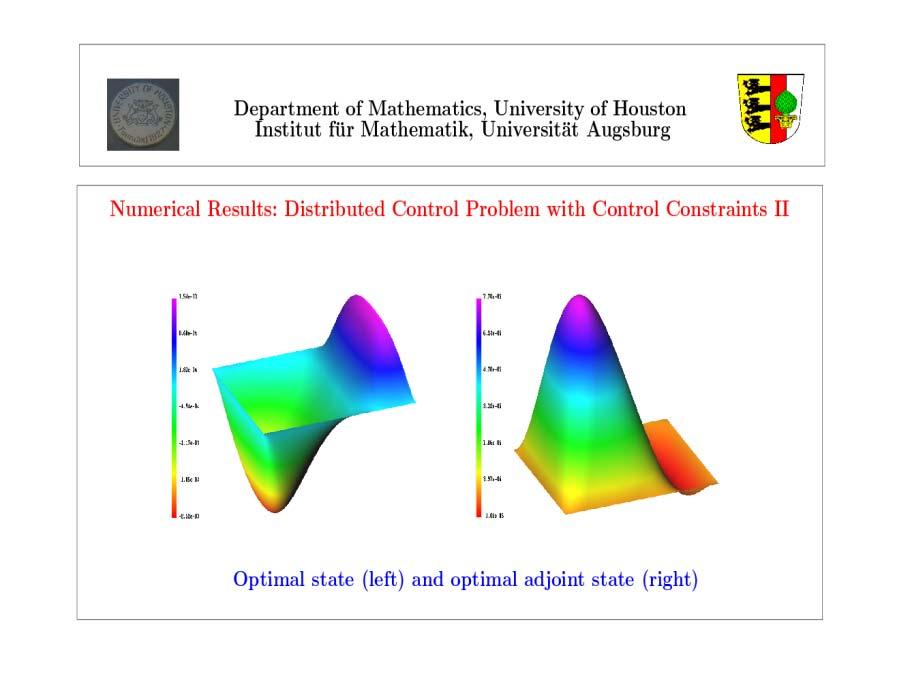
48 Numerical Results: Adaptive FEM for a Distributed Control Problem Initial triangulation and triangulation after 6 refinement steps ( Θ = 0.6)

49 Numerical Results: Distributed Control Problem with Control Constraints I l N dof z z H y y H 1 p p H 1 u u H 0 λ λ H e e e e e e e e e e e e e e e e e e e e e e e e e e e e e e e e e e e e e e e e e e e e e-05 Total error, errors in the state, adjoint state, control, adjoint control (Θ = 0.7)

50 Numerical Results: Distributed Control Problem with Control Constraints I l N dof η y η p osc h (y d ) e e e e e e e e e e e e e e e e e e e e e e e e e e e-05 Components of the error estimator and data oscillations (Θ = 0.7)

51 Numerical Results: Distributed Control Problem with Control Constraints II Minimize J(y,u) := 1 2 y yd 2 0,Ω + α 2 u ud 2 0,Ω over (y,u) H 1 0(Ω) L 2 (Ω) subject to y = f + u in Ω, u K := {v L 2 (Ω) v ψ a.e. in Ω} û := Data: Ω := (0,1) 2, y d := 0, u d := û + α 1 (ˆσ + 2 û), (x ψ := 1 0.5) 8, (x 1,x 2 ) Ω 1, (x 1 0.5) 2, α := 0.1, f := 0, otherwise ψ, (x 1,x 2 ) Ω 1 Ω 2, 1.01 ψ, otherwise, ˆσ := 2.25 (x ) 10 4, (x 1,x 2 ) Ω 2, 0, otherwise Ω 1 := {(x 1,x 2 ) Ω ((x 1 0.5) 2 + (x 2 0.5) 2 ) 1/2 0.15}, Ω 2 := {(x 1,x 2 ) Ω x }.,

52

53

54 Numerical Results: Distributed Control Problem with Control Constraints II Grid after 6 (left) and 8 (right) refinement steps ( Θ = 0.6)

55 Numerical Results: Distributed Control Problem with Control Constraints II l N dof z z H y y H 1 p p H 1 u u H 0 λ λ H e e e e e e e e e e e e e e e e e e e e e e e e e e e e e e e e e e e e e e e e e e e e e-07 Total error, errors in the state, adjoint state, control, adjoint control (Θ = 0.6)

56 Numerical Results: Distributed Control Problem with Control Constraints II Decrease in the quantity of interest versus total number of DOFs

57 Department of Mathematics, University of Houston The Goal Oriented Dual Weighted Approach for State Constrained Elliptic Optimal Control Problems Ronald H.W. Hoppe 1,2 1 Department of Mathematics, University of Houston 2 Institute of Mathematics, University of Augsburg Mathematisches Forschungsinstitut Oberwolfach Oberwolfach, November 2010

58 Department of Mathematics, University of Houston Goal-Oriented Dual Weighted Approach

59 Goal-Oriented Dual Weighted Approach I The goal oriented dual weighted approach allows to control the error e u := u u h with respect to a rather general error functional or output functional J : V H 1 (Ω) lr. The goal oriented dual weighted approach strongly uses the solution z V of the associated dual problem a(v,z) = J(v), v V, and its finite element approximation z h V h, i.e., a(v h,z h ) = J(v h ), v h V h. Using Galerkin orthogonality, we readily deduce that J(e u ) = a(e u,z) = a(e u,z v h ) = r(z v h ), v h V h, where r( ) stands for the residual with respect to the computed finite element approximation u h.

60 Goal-Oriented Dual Weighted Approach II Theorem. Let u h V h := S 1,Γ (Ω; T h (Ω)) be the conforming P1 approximation of the solution u H 1 0(Ω) of Poisson s equation with f L 2 (Ω) and homogeneous Dirichlet boundary data. Then, the following error representation holds true J(e u ) = ) ((r T,z v h ) 0,T + (r T,z v h ) 0, T, v h V h, T T h (Ω) where the element residuals r T and the edges residuals r T are given by { 1 r T := f, T T h (Ω), r T E := 2 ν E [ u h ], E E h ( T Ω) 0, E E h ( T Γ) Moreover, we have the error estimate J(e u ) η DW := ω T ρ T, T T h (Ω) where for v h V h the element residuals ρ T and the weights ω T read ( 1/2, ( 1/2. ρ T := r T 2 0,T + h 1 T r T 0, T) 2 ωt := z v h 2 0,T + h T z v h 0, T) 2

61 Department of Mathematics, University of Houston Goal-Oriented Dual Weighted Approach III We remark that the previous result is not really a posteriori, since the solution z V of the dual solution is not known. Therefore, information about the weights ω T,T T h (Ω) has to be provided either by means of an a priori analysis or by the numerical solution of the dual problem. Theorem. Under the assumptions of the previous theorem let the error functional be given by Then, there holds J(v) := ( v, e u) 0,Ω e u 0,Ω, v V. e u 0,Ω C ( T T h (Ω) h 2 T ρ 2 T) 1/2.

62 Proof. The dual solution z V satisfies a(v,z) = ( v, e u) 0,Ω e u 0,Ω, v V, from which we readily deduce the a priori bound z 0,Ω 1. In view of the basic error estimate it follows that ( ) 1/2 ( J(e u ) = e u 0,Ω h 2 T ρ 2 T T T h (Ω) T T h (Ω) h 2 T ω2 T) 1/2. Choosing v h = P C z, where P C is Clément s quasi-interpolation operator, we find ( 1/2 inf (h 2 T z v h 2 0,T + h 1 T z v h 0, T) 2 C z 0,Ω. v h V h T T h (Ω) Using the last inequality in the previous one and observing the error representation gives the assertion.

63 Goal-Oriented Dual Weighted Approach IV Theorem. Consider the conforming P1 approximation of Poisson s equation under homogeneous Dirichlet boundary conditions and assume that the solution u V := H 1 0(Ω) is 2-regular. Using the the error functional J(v) := (v,e u) 0,Ω e u 0,Ω, v V, gives rise to the a posteriori error estimate ( e u 0,Ω C T T h (Ω) h 4 T ρ 2 T) 1/2.

64 Goal-Oriented Dual Weighted Approach V Finally, we apply the goal-oriented dual weighted approach to the pointwise estimation of the error at some point a Ω. Given some tolerance ε > 0, we consider the ball K ε (a) := {x Ω x a < ε} around the point a and define the regularized error functional J(v) := Kε(a) 1 v dx. Kε (a) The dual solution z of a(v,z) = J(v) behaves like a regularized Green s function With the residual ρ T we obtain z(x) log(r(x)), r(x) := x a 2 + ε 2. (u u h )(a) T T h (Ω) h 3 T r 2 T ρ T, r T := max x T r(x).

65 Department of Mathematics, University of Houston Goal-Oriented Dual Weighted Approach for State Constrained Elliptic Optimal Control Problems

66 Department of Mathematics, University of Houston C O N T E N T S Representation of the error in the quantity of interest Primal-Dual Weighted Residuals Primal-Dual Mismatch in Complementarity Primal-Dual Weighted Data Oscillations Numerical Results

67 Department of Mathematics, University of Houston State Constrained Elliptic Control Problems

68 Literature on State-Constrained Optimal Control Problems M. Bergounioux, K. Ito, and K. Kunisch (1999) M. Bergounioux, M. Haddou, M. Hintermüller, and K. Kunisch (2000) M. Bergounioux and K. Kunisch (2002) E. Casas (1986) E. Casas and M. Mateos (2002) J.-P. Raymond and F. Tröltzsch (2000) K. Deckelnick and M. Hinze (2006) M. Hintermüller and K. Kunisch (2007) K. Kunisch and A. Rösch (2002) C. Meyer and F. Tröltzsch (2006) C. Meyer, U. Prüfert, and F. Tröltzsch (2005) U. Prüfert, F. Tröltzsch, and M. Weiser (2004) H./M. Kieweg (2007) A. Günther, M. Hinze (2007) O. Benedix, B. Vexler (2008) M. Hintermüller/H. (2008) W. Liu, W. Gong and N. Yan (2008)

69 Model Problem (Distributed Elliptic Control Problem with State Constraints) Let Ω lr 2 be a bounded domain with boundary Γ = Γ D Γ N, Γ D Γ N =, and let A : V H 1 (Ω), V := {v H 1 (Ω) v Γd = 0}, be the linear second order elliptic differential operator Ay := y + cy, c 0, with c > 0 or meas(γ D ) > 0. Assume that Ω is such that for each v L 2 (Ω) the solution y of Ay = u satisfies y W 1,r (Ω) V for some r > 2. Moreover, let u d,y d L 2 (Ω), and ψ W 1,r (Ω) such that ψ ΓD > 0 be given functions and let α > 0 be a regularization parameter. Consider the state constrained distributed elliptic control problem Minimize J(y,u) := 1 2 y yd 2 0,Ω + α 2 u ud 2 0,Ω, subject to Ay = u in Ω, y = 0 on Γ D, ν y = 0 on Γ N, Iy K := {v C(Ω) v(x) ψ(x), x Ω}. where I stands for the embedding operator W 1,r (Ω) C(Ω).

70 Department of Mathematics, University of Houston We introduce the control-to-state map The Reduced Optimal Control Problem G : L 2 (Ω) C(Ω), y = Gu solves Ay + cy = u. We assume that the following Slater condition is satisfied (S) There exists v 0 L 2 (Ω) such that Gv 0 int(k). Substituting y = Gu allows to consider the reduced control problem inf u U ad J red (u) := 1 2 Gu yd 2 0,Ω + α 2 u ud 2 0,Ω, U ad := {v L 2 (Ω) (Gv)(x) ψ(x), x Ω}. Theorem (Existence and uniqueness). The state constrained optimal control problem admits a unique solution y W 1,r (Ω) K.

71 Optimality Conditions for the State Constrained Optimal Control Problem Theorem. There exists an adjoint state p V s := {v W 1,s (Ω) v ΓD = 0}, where 1/r + 1/s = 1, and a multiplier σ M + (Ω) such that ( y, v) 0,Ω + (cy,v) 0,Ω = (u,v) 0,Ω, v V s, ( p, w) 0,Ω + (cp,w) 0,Ω = (y y d,w) 0,Ω + σ,w, w Vr, p + α(u u d ) = 0, σ,y ψ = 0.

72 Department of Mathematics, University of Houston Proof. The reduced problem can be written in unconstrained form as inf Ĵ(v) := J red (v) + (I K G)(u) v L 2 (Ω) where I K stands for the indicator function of the constraint set K. The Slater condition and and subdifferential calculus tell us ( ) I K G (u) = G I K (Gu). The optimality condition then reads 0 Ĵ(u) = J red (u) + G I K (Gu). Hence, there exists σ I K (Gu) such that ( ) G (Gu y d + σ) +α(u u }{{} d ),v = 0, v 0,Ω L2 (Ω). =: p Since σ M(Ω), PDE regularity theory implies p W 1,s (Ω),1/s + 1/r = 1.

73 Department of Mathematics, University of Houston Finite Element Approximation Let T l (Ω) be a simplicial triangulation of Ω and let V l := { v l C(Ω) v l T P 1 (T), T T l (Ω), v l ΓD = 0 } be the FE space of continuous, piecewise linear functions. Let u d l V l be some approximation of ud, and let ψ l be the V l -interpoland of ψ. Consider the following FE Approximation of the state constrained control problem Minimize J l (y l,u l ) := 1 2 y l yd 2 0,Ω + α 2 u l ud l 2 0,Ω, over (y l,u l ) V l V l, subject to ( y l, v l ) 0,Ω + (cy l,v l ) 0,Ω = (u l,v l ) 0,Ω, v l V l, y l K l := {v l V l v l (x) ψ l (x), x Ω}. Since the constraints are point constraints associated with the nodal points, the discrete multipliers are chosen from M l := {µ l M(Ω) µ l = a N l (Ω Γ N ) κ a δ a, κ a lr}.

74 Department of Mathematics, University of Houston Representation of the Error in the Quantity of Interest

75 Department of Mathematics, University of Houston Primal-Dual Weighted Error Representation I We set X := V r L 2 (Ω) V s as well as X l := V l V l V l and introduce the Lagrangians L : X M(Ω) lr as well as L l : X l M l lr according to L(x, σ) := J(y,u) + ( y, p) 0,Ω (u,p) 0,Ω + σ,y ψ, L l (x l, σ l ) := J l (y l,u l ) + ( y l, p l ) 0,Ω (u l,p l ) 0,Ω + σ l,y l ψ l, where x := (y,u,p) and x l := (y l,u l,p l ). Then, the optimality conditions can be stated as x L(x, σ)(ϕ) = 0, ϕ X, x L l (x l, σ l )(ϕ l ) = 0, ϕ l X l.

76 Department of Mathematics, University of Houston Primal-Dual Weighted Error Representation II Theorem. Let (x, σ) X and (x l, σ l ) X l be the solutions of the continuous and discrete optimality systems, respectively. Then, there holds J(y,u) J l (y l,u l ) = 1 2 xxl(x l x,x l x) + σ,y l ψ + osc (1) l, where the data oscillations osc (1) l are given by osc (1) l := osc (1) T T l (Ω) T, osc (1) T := (y l y d l,yd l yd ) 0,T yd y d l 2 0,T + α (u l u d l,ud l ud ) 0,T + α 2 ud u d l 2 0,T. Remark: In the unconstrained case, i.e., σ = σ l = 0, the above result reduces to the error representation in [Becker, Kapp, and Rannacher (2000)].

77 Department of Mathematics, University of Houston Interpolation Operators (State Constraints) We introduce interpolation operators i y l : V r V l, r > r > 2, i p l : V s V l, 0 < s < s < 2, such that for all y V r and p V s there holds ( ( ( h r(t 1) T i y l y y r t,r,t h r T iy l y y r 0,r,T + h r/2 T h s T ip l p p s 0,s,T + h s/2 T where D T := {T T l (Ω) N l (T ) N l (T) }. ) 1/r y 1,r,DT, 0 t 1, i y l y y r 0,r, T i p l p p s 0,s, T ) 1/r y 1,r,DT, ) 1/s h T p 1,s,DT, 1

78 Primal-Dual Weighted Error Representation III Theorem. Under the assumptions of the previous Theorem let i z l,z {y,p}, be the interpolation operators introduced before. Then, there holds J(y,u) J l (y l,u l ) = (r(i y l y y) + r(ip l p p)) + µ l (x, σ) + osc(1) l where r(i y l y y) and r(ip l p p) stand for the primal-dual weighted residuals + osc (2) l, r(i y l y y) := 1 2 ((y l yd l,iy l y y) 0,Ω + ( (i y l y y, p l ) 0,Ω + σ l,i y l y y ), r(i p l p p) := 1 2 (( (ip l p p, y l ) 0,Ω (u l,i p l p p) 0,Ω). Moreover, µ l (x, σ) represents the primal-dual mismatch in complementarity and osc (2) l osc (2) l are further oscillation terms := µ l (x, σ) := 1 2 ( σ,y l ψ + σ l, ψ l y ), T T l (Ω) osc (2) T, osc (2) T := 1 2 ((yd y d l,y l y) 0,T + α (u d u d l,u l u) 0,T).

79 Department of Mathematics, University of Houston Primal-Dual Weighted Residuals

80 Primal-Dual Weighted Residuals Theorem. The primal-dual residuals can be estimated according to r(i y l y y) C ( ω y T ρy T + ωσ T ρ σ ) T, r(i p l p p) C ω p T ρp T. T T l (Ω) T T l (Ω) Here, ρ y T and ρp T are Lr -norms and L s -norms of the residuals associated with the state and the adjoint state equation ( ρ y T := u l r 0,r,T + h r/2 T 1 ) 1/r 2 ν [ y l ] r 0,r, T, ( ρ p T := y l y l d s 0,s,T + h s/2 T 1 ) 1/s 2 ν [ p l ] s 0,s, T. The corresponding dual weights ω y T and ωp T are given by ( ) 1/s ω y T := i p l p p s 0,s,T + h s/2 T ip l p p s 0,s, T, ( ) 1/r ω p T := i y l y y r 0,r,T + h r/2 T iy l y y r 0,r, T. The residual ρ σ T and its dual weight ωσ T are given by ρ σ T := n 1 a κ a, ω σ T := i y l y y 2/r+ε,r,T, 0 < ε < (r 2)/r. a N l (T)

81 Department of Mathematics, University of Houston Primal-Dual Mismatch in Complementarity

82 Department of Mathematics, University of Houston Primal-Dual Mismatch in Complementarity The primal-dual mismatch µ l (x, σ) can be made partially a posteriori in the following two particular cases (cf. [Bergounioux/Kunisch (2003)]): Regular Case Nonregular Case The active set A is the union of a finite num- The active set A is a Lipschitzian curve ber of mutually disjoint, connected sets A i, that divides Ω into two connected com- 1 i m, with C 1,1 -boundary. ponents Ω + and Ω. p I H 2 (I), p int(a) H 2 (int(a)) ( p, w) 0,Ω = (y d y,w) σ,w, w V r p = y d y in I, p = α ψ in A { 0 on I σ A = y d ψ α 2 ψ on A σ = σ A + σ F, σ F = p I ν I + α ψ ν A σ = σ A := ν A p A+ ν A p A

83 Department of Mathematics, University of Houston Primal-Dual Mismatch in Complementarity The primal-dual mismatch in complementarity has the representations µ l I Il = 1 2 (σ F,y l ψ) 0,F Il µ l I Al = 1 2 (σ F, ψ l ψ) 0,F Al a N l (F l I) a N l (I A l ) κ a (y l y)(a), κ a (ψ l y)(a), µ l A Il = 1 2 (σ F,y l ψ) 0,F Il (yd ψ α 2 ψ,y l ψ) 0,A Il, µ l A Al = 1 2 (σ F, ψ l ψ) 0,F Al (yd ψ α 2 ψ, ψ l ψ) 0,A Al. Hence, we need appropriate approximations of the continuous coincidence set A, the continuous non-coincidence set I, the continuous free boundary F, and of σ F.

84 Department of Mathematics, University of Houston Primal-Dual Mismatch in Complementarity (State Constraints) The coincidence set A and the non-coincidence set I will be approximated by  l := {T T l χ A l (x) 1 κh for all x T}, where Î l := {T T l χ A l (x) 1 κh for some x T}, χ A l := I ψ i y l y l γh r + ψ i y l y l, 0 < γ 1, r > 0. Note that for T A we have ( ) χ(a) χ A l 0,T min T 1/2, γ 1 h r y i y l y 0,T 0 for y i y l y 0,T = O(h q ), q > r. Moreover, σ F will be approximated by σ ˆF l := { νîl p l Îl + α νâl ψ, E T l (Â) T l (Î) νâl p l Âl,+ νâl p l Âl,, E E l (Â) \ ( T l (Â) T l (Î)).

85 Primal-Dual Mismatch in Complementarity (State Constraints) The primal-dual mismatch in complementarity can be estimated from above as follows: µ l I Il ˆµ (1) l + ˆµ(2) l, µ l I A l ˆµ (1) l + ˆµ(3) l, µ l A I l ˆµ (1) l + ˆµ(4) l, µ l A A l ˆµ (1) l + ˆµ(5) l. where ˆµ (1) := ˆµ (1) l E, ˆµ (1) E := 1 2 σ ˆF l 0,E y l ψ 0,E, ˆµ (2) l := ˆµ (3) l := ˆµ (4) l := ˆµ (5) l := E E l ( ˆF l ) E E l (F l Î l ) T T l (Î l A l ) T T l ( l I l ) T T l ( l A l ) ˆµ (2) E, ˆµ (2) E := 1 2 ˆµ (3) T, ˆµ (3) T := 1 2 a N l (E) a N l (T) (y l i y l y l )(a) κ a, y l i y l y l )(a) κ a,, ˆµ (4) T, ˆµ (4) T := 1 2 yd ψ α 2 ψ 0,T y l ψ 0,T, ˆµ (5) T, ˆµ (5) T := 1 2 yd ψ α 2 ψ 0,T ψ l ψ 0,T.

86 Department of Mathematics, University of Houston Primal-Dual Weighted Data Oscillations

87 Department of Mathematics, University of Houston Primal-Dual Weighted Data Oscillations The data oscillations osc (2) l := osc (2) l T T l (Ω) as given by osc (2) T, osc (2) T := 1 2 ( ) (y d y l d,y l y) 0,T + α (u d u d l,u l u) 0,T can be estimated from above according to osc (2) ôsc (2) l T, ôsc (2) T := ˆωp T ud u d l 0,T + ˆω y T yd y l d 0,T + α u d u d l 2 0,T, T T l (Ω), where the weights ˆω p T and ˆωy T are given by ˆω p T := ip l p l p l 0,T, ˆω y T := iy l y l y l 0,T.

88 Department of Mathematics, University of Houston State Constraints: Numerical Results

89 Numerical Results: Distributed Control Problem with State Constraints I Minimize J(y,u) := 1 2 y yd 2 0,Ω + α 2 u ud 2 0,Ω over (y,u) H 1 0(Ω) L 2 (Ω) subject to y = u in Ω, y K := {v H 1 0(Ω) v ψ a.e. in Ω} Data: Ω := ( 2, +2) 2, y d (r) := y(r) + p(r) + σ(r), u d (r) := u(r) + α 1 p(r), ψ := 0, α := 0.1, where y(r),u(r),p(r), σ(r) is the solution of the problem: y(r) := r 4/3 + γ 1 (r), u(r) = y(r), p(r) = γ 2 (r) + r r r2, σ(r) :=, γ 1 := γ 2 := 1, r < (r 0.25) (r 0.25) 4 80(r 0.25) 3 + 1, 0.25 < r < , otherwise { 1, r < , otherwise. { 0.0, r < , otherwise,

90 Numerical Results: Distributed Control Problem with State Constraints I Optimal state (left) and optimal control (right)

91 Numerical Results: Distributed Control Problem with State Constraints I 10 3 J(y *,u * ) - J h (y * h,u* h ) θ = 0.3 uniform Decrease in the quantity of interest versus total number of DOFs N

92 Department of Mathematics, University of Houston Numerical Results: Distributed Control Problem with State Constraints II Minimize J(y,u) := 1 2 y yd 2 0,Ω + α 2 u ud 2 0,Ω over (y,u) H 1 (Ω) L 2 (Ω) subject to y + cy = u in Ω, y K := {v H 1 (Ω) v ψ a.e. in Ω} Data: Ω = B(0,1) := {x = (x 1,x 2 ) T x x 2 2 < 1}, y d (r) := π 1 4π r π ln(r), u d (r) := π r2 1 ln(r), ψ := 4 + r, α := 1. 2π The solution y(r),u(r),p(r), σ(r) of the problem is given by y(r) 4, u(r) 4, p(r) = 1 4π r2 1 2π ln(r), σ(r) = δ 0.

93 Numerical Results: Distributed Control Problem with State Constraints II Optimal state (left) and optimal control (right)

94 Numerical Results: Distributed Control Problem with State Constraints II Optimal adjoint state (left) and mesh after 16 adaptive loops (right)

95 Numerical Results: Distributed Control Problem with State Constraints II θ = 0.3 uniform J(y *,u * ) - J h (y * h,u* h ) Decrease in the quantity of interest versus total number of DOFs N

96 Department of Mathematics, University of Houston Control Constrained Elliptic Control Problems

97 Department of Mathematics, University of Houston A Posteriori Error Analysis of AFEM for Optimal Control Problems (i) Unconstrained problems R. Becker, H. Kapp, R. Rannacher (2000) R. Becker, R. Rannacher (2001) (ii) Control constrained problems W. Liu and N. Yan (2000/01) R. Li, W. Liu, H. Ma, and T. Tang (2002) M. Hintermüller/H. et al. (2006) A. Gaevskaya/H. et al. (2006/07) A. Gaevskaya/H. and S. Repin (2006/07) M. Hintermüller/H. (2007) B. Vexler and W. Wollner (2007)

98 Department of Mathematics, University of Houston Model Problem (Distributed Elliptic Control Problem with Control Constraints) Given a bounded domain Ω R 2 with polygonal boundary Γ = Ω, a function y d, ψ L 2 (Ω), and α > 0, consider the distributed optimal control problem Minimize J(y,u) := 1 2 y yd 2 0,Ω + α 2 u 2 0,Ω, over (y,u) H 1 0(Ω) L 2 (Ω), subject to y = u, u K := {v L 2 (Ω) v ψ a.e. in Ω}. 1

99 Department of Mathematics, University of Houston Optimality Conditions for the Distributed Control Problem There exists an adjoint state p H 1 0(Ω) and an adjoint control σ L 2 (Ω) such that the quadruple (y, p, u, σ) satisfies a(y,v) = (u,v) 0,Ω, v H1 0(Ω), a(p,v) = (y d y,v) 0,Ω, v H1 0(Ω), α u = p σ, σ 0, u ψ, (σ;u ψ) 0,Ω = 0, where a(, ) stands for the bilinear form a(w, z) = w z dx, w,z H 1 0(Ω). Ω 1

100 Finite Element Approximation of the Distributed Control Problem Let T l (Ω) be a shape regular, simplicial triangulation of Ω and let V l := { v l C(Ω) v l T P k1 (T), T T l (Ω), k 1 N, v H Ω = 0 } be the FE space of continuous, piecewise polynomial functions (of degree k 1 ) and W l := { w l L 2 (Ω) w l T P k2 (T), T T l (Ω), k 2 N {0} } the linear space of elementwise polynomial functions (of degree k 2 ). Consider the following FE Approximation of the distributed control problem Minimize J l (y l,u l ) := 1 2 y l yd l 2 0,Ω + α 2 u l 2 0,Ω, over (y l,u l ) V l W l, subject to a(y l,v l ) = (u l,v l ) 0,Ω, v l V l, u l K l := {w l W l w l T ψ l T, T T l (Ω)}. where ψ l W l is the discrete control constraint. 1

101 Department of Mathematics, University of Houston Optimality Conditions for the FE Discretized Control Problem There exists an adjoint state p l V l and an adjoint control σ l W l such that the quadruple (y l,u l,p l, σ l ) satisfies a(y l,v l ) = (u l,v l ) 0,Ω, v l V l, a(p l,v l ) = (y d l y,v l ) 0,Ω, v l V l, α u l = M l p l σ l, σ l 0, u l ψ l, (σ l,u l ψ l ) 0,Ω = 0, where y d l V l and M l : V l W l, e.g., for k 2 = 0: (M l v l ) T := T 1 v l dx, T T l (Ω). T 1

102 Primal-Dual Weighted Error Representation (Control Constraints) Theorem. Let (x, σ) X L 2 (Ω) and (x l, σ l ) X l W l be the solutions of the continuous and discrete optimality systems, respectively. Then, there holds J(y,u) J l (y l,u l ) = 1 2 xxl(x l x,x l x) + (σ,u l ψ) 0,Ω + osc(1) l. Remark: In the unconstrained case, i.e., σ = σ l = 0, the above result reduces to the error representation in [Becker, Kapp, and Rannacher (2000)].

103 Primal-Dual Weighted Error Representation (Control Constraints) Theorem. Under the assumptions of the previous Theorem let i z l,z {y,u,p}, be the interpolation operators introduced before. Then, there holds ) J(y,u) J l (y l,u l ) = (r(i y l y y) + r(ip l p p) + r(iu l u u) + µ l (x, σ) + osc (1) l + osc (2) l, where r(i y l y y), r(ip l p p) and r(iu l u u) stand for the primal-dual weighted residuals r(i y l y y) := 1 ( ) (y 2 l y l d,iy l y y) 0,Ω + ( (i y l y y), p l ) 0,Ω, r(i p l p p) := 1 ( ) ( (i p 2 l p p), y l ) 0,Ω (u l,i p l p p) 0,Ω, r(i u l u u) := 1 2 (M l p l p l,iu l u u) 0,Ω. Moreover, µ l (x, σ) represents the primal-dual mismatch in complementarity µ l (x, σ) := 1 ( ) (σ,u 2 l ψ) 0,Ω + (σ l, ψ l u) 0,Ω, and osc (2) l is a further oscillation term osc (2) := osc (2) l T, osc (2) T := 1 2 (yd y l d,y l y) 0,T. T T l (Ω)

104 Primal-Dual Weighted Residuals (Control Constraints) Theorem. The primal-dual residuals can be estimated according to r(i y l y y) C ω y T ρy T, r(i p l p p) C ( ) ω p T ρp,1 T + ω u Tρ p,2 T. T T l (Ω) T T l (Ω) Here, ρ y T and ρp,1 T are L2 -norms of ( the residuals associated with the ) state and the adjoint state 1/2 ρ y T := u l 2 0,T + h 1 T 1 2 ν [ y l ] 2 0, T, ( ) 1/2 ρ p,1 T := y l y l d 2 0,T + h 1 T 1 2 ν [ p l ] 2 0, T. The corresponding dual weights ω u T and ωp T are given by ( ) 1/2 ω y T := i p l p p 2 0,T + h T i p l p p 2 0, T, ( ) 1/2 ω p T := i y l y y 2 0,T + h T i y l y y 2 0, T. The residual ρ p,2 T and its dual weight ωu T are given by ρ p,2 T := M l p l p l 0,T, ω u T := i u l u u 0,T.

105 Primal-Dual Mismatch in Complementarity (Control Constraints) Using the complementarity conditions u ψ, σ 0, (σ,u ψ) 0,Ω = 0, αu p + σ = 0, u l ψ l, σ l 0, (σ l,u l ψ l ) 0,Ω = 0, αu l M l p l + σ l = 0, the primal-dual mismatch µ l := µ l (x, σ) can be further assessed according to µ l (I I l ) = 0, µ l (A A l ) = 1 2 (σ + σ l, ψ l ψ) 0,A A l, µ l (I A l ) = 1 2 (σ l, ψ l α 1 p) 0,I Al, µ l (A I l ) = α 2 u u l 2 0,I A l (p M l p l,u l u) 0,I A l. and we finally obtain µ l (I A l ) + µ l (A I l ) ν l with a fully computable a posteriori term ν l (consistency error).

106 Numerical Results: Distributed Control Problem with Control Constraints I Minimize J(y,u) := 1 2 y yd 2 0,Ω + α 2 u 2 0,Ω over (y,u) H 1 0(Ω) L 2 (Ω) subject to y = u in Ω, u K := {v L 2 (Ω) v ψ a.e. in Ω} Data: Ω := (0,1) 2, { y d 200 x := 1 x 2 (x 1 0.5) 2 (1 x 2 ), 0 x (x 1 1) (x 2 (x 1 0.5) 2 (1 x 2 ), 0.5 < x 1 1, α = 0.01, ψ = 1.

107 Numerical Results: Distributed Control Problem with Control Constraints I Optimal state (left) and optimal control (right)

108 Numerical Results: Distributed Control Problem with Control Constraints I Grid after 6 (left) and 10 (right) refinement steps

109 Numerical Results: Distributed Control Problem with Control Constraints I l N dof δ h η h osc h ν h E E E E E E E E E E E E E E E E E E E E E E E E E E E E E E E E E E E E E E E E-09 Error (quantity of interest), estimator, oscillations, and consistency error

110 Numerical Results: Distributed Control Problem with Control Constraints II Minimize J(y,u) := 1 2 y yd 2 0,Ω + α 2 u ud 2 0,Ω over (y,u) H 1 0(Ω) L 2 (Ω) subject to y = f + u in Ω, u K := {v L 2 (Ω) v ψ a.e. in Ω} Data: Ω := (0,1) 2, y d := 0, u d := û + α 1 (ˆσ 2 û), { (x1 0.5) ψ := 8, (x 1,x 2 ) Ω 1, (x 1 0.5) 2, α := 0.1, f := 0, otherwise { { ψ, (x û := 1,x 2 ) Ω 1 Ω 2, 2.25 (x1 0.75) 10, ˆσ := 4, (x 1,x 2 ) Ω 2, 1.01 ψ, otherwise 0, otherwise ( ) 1/2 Ω 1 := {(x 1,x 2 ) Ω (x 1 0.5) 2 + (x 2 0.5) }, Ω2 := {(x 1,x 2 ) Ω x }.,

111 Numerical Results: Distributed Control Problem with Control Constraints II Optimal state (left) and optimal control (right)

112 Numerical Results: Distributed Control Problem with Control Constraints II Grid after 6 (left) and 10 (right) refinement steps

113 Numerical Results: Distributed Control Problem with Control Constraints I l N dof δ h η h osc h ν h E E E E E E E E E E E E E E E E E E E E E E E E E E E E E E E E E E E E E E E E-16 Error (quantity of interest), estimator, oscillations, and consistency error

114 Numerical Results: Distributed Control Problem with Control Constraints II Decrease in the quantity of interest versus total number of DOFs

115 Department of Mathematics, University of Houston Elliptic Optimal Control Problems Constraints on the Gradient of the State

116 Elliptic Optimal Control with Pointwise Gradient-State Constraints Let Ω R 2 be a bounded polygonal domain with boundary Γ, y d L 2 (Ω) a desired state, f a forcing term, ψ L 2 (Ω) s.th. ψ ψ min > 0 a.e. in Ω, and α > 0, find (y,u) H 1 0(Ω) L 2 (Ω) such that (P) inf J(y,u) := 1 y y d 2 dx + α u 2 dx, (y,u) 2 2 subject to Ly := a y + cy = f + u in Ω, y = 0 on Γ, y K := {v L 2 (Ω) 2 v ψ a.e. in Ω}. Ω Ω

117 Pointwise Gradient-State Constraints: State-Reduced Formulation Let ˆV H 1 0(Ω) be a reflexive Banach space and let Ĝ : L 2 (Ω) ˆV be the map that assigns to the rhs f + u the solution y = Ĝ(f + u) of the state equation. Assume that Ĝ is a bounded linear operator which is invertible such that u = Ĝ 1 y f. This leads to the state-reduced formulation: Find y ˆK := {v ˆV v ψ bf a.e. in Ω} such that inf J red (y) := 1 2 y ˆK Unconstrained formulation: Ω y y d 2 dx + α 2 inf J red (y) + IˆK (y) y ˆV where IˆK stands for the indicator function of the set ˆK. Ω Ĝ 1 y f 2 dx.

118 State-Reduced Formulation: Optimality Conditions Theorem. The gradient-state constrained optimal control problem admits a unique solution (y,u) ˆK L 2 (Ω) which is characterized by the existence of a unique pair (p,w) L 2 (Ω) ˆV satisfying Lp = (a p) + cp = y d y w in ˆV, p = αu in L 2 (Ω), w NˆK (y) := {ξ ˆV ξ,z y ˆV,ˆV 0, z ˆK}. Remark. If ˆV = W 2,r (Ω) H 1 0(Ω),r > 2, there exists a Slater point, i.e., y 0 int ˆK and (y 0 + v) ψ in Ω for all v C 1 ( Ω) s.th. v C 1 ( Ω) δ for sufficiently small δ > 0. 0 J red(y) + (IˆK )(y) = J red(y) IˆK ( y), i.e., there exists µ IˆK ( y) M( Ω) 2 such that w = µ.

119 Control-Reduced Formulation and Dual Problem Denoting by G : H 1 (Ω) H 1 0(Ω) the solution operator associated with the state equation, the optimal control problem can be written according to where inf F(u) + G(Λu) u L 2 (Ω) F(u) := J(G(f + u),u), G(q) := I K (q), Λ := G. Denoting by F and G the Fenchel conjugates of F and G F (u ) = 1 2 u + G y d + αf 2 M 1, G (q ) = ψ q dx, where M := G G + αi and 2 := (M 1, ) M 1 0,Ω, the dual problem reads as follows: (D) sup F (Λ q ) G ( q 1 ) inf 2 G ( µ + y d ) + αf 2 M 1 + ψ µ dx. q L 2 (Ω) µ L 2 (Ω) Ω Ω

120 Department of Mathematics, University of Houston Tightened Formulation of the Primal Problem Consider the following tightened formulation of the primal problem (ˆP) inf J(y,u) := 1 y y d 2 dx + α u 2 dx, (y,u) ˆV L 2 (Ω) 2 2 subject to Ω Ω Ly = f + u in Ω, y = 0 on Γ, y ψ a.e. in Ω. Theorem. Let {µ n } N L 2 (Ω) 2 be a minimizing sequence for the dual (ˆD) to (ˆP). Then, there exist a subsequence {µ n } N and µ M( Ω) 2 such that w lim µ n = µ in M( Ω) 2 and w lim µ n = w in ˆV. Moreover, the limit w ˆV satisfies ( ) Ly = f + u in L 2 (Ω), Lp = y d y w in ˆV, p = αu in L 2 (Ω). Remark. A quadruple (y,u,p,w) V L 2 (Ω) L 2 (Ω) ˆV such that ( ) holds true and y (M( Ω) 2 ) \ C( Ω) 2, is called a weak solution of (P).

121 Finite Element Discretization of (P) and (ˆP) Let T h (Ω) be a simplicial triangulation of Ω and denote by E h (D) the set of edges of T h (Ω) in D Ω. We refer to V h := {v h C 0 (Ω) v h T P 1 (T),T T h (Ω)} as the finite element space of P1 conforming FEs w.r.t. T h (Ω) and set W h := {w h : Ω R 2 w h T P 0 (T) 2,T T h (Ω)}. We define ψ h according to ψ h T := T 1 T ψdx,t T h(ω) and set K h := {z h W h z h T ψ h T, T T h (Ω)}. The discrete optimal control problems reads: (ˆP h ) inf J(y h,u h ) := 1 y h y d 2 dx + α (y h,u h ) 2 2 Ω Ω u h 2 dx, subject to a(y h,v h ) = (f + u h,v h ) 0,Ω, v h V h, y h K h.

122 Discrete Optimal Control Problem: Optimality Conditions Theorem. The discrete optimal control problem (ˆP h ) admits a unique solution (y h,u h ) V h V h which is characterized by the existence of an adjoint state p h V h and a multiplier µ h W h such that a(p h,v h ) (y d y h,v h ) 0,Ω + (µ h T, v h T ) 0,T = 0, v h V h, T T h (Ω) T T h (Ω) p h αu h = 0, (µ h T,q h T y h T ) 0,T 0, q h K h. Remark. The Fenchel dual associated with (ˆP h ) reads 1 (ˆD h ) inf 2 G h( µ h + y d ) + αf 2 M 1 + h µ h W h Ω ψ h µ h dx.

123 Prager-Synge Equilibration (cf. Braess/Schöberl (08), Braess/H./Schöberl (09)) Construct µ h RT 0 (Ω; T h (Ω)) such that σ i,j,r σ i,j,l (µ h T, v h T ) 0,T = (n E [µ h ] E,v h ) 0,E σ i,j+1,r σ i,j+1,l T T h (Ω) = T T h (Ω) E E h (Ω) ( µ h,v h ) 0,T, v h V h. Then the discrete optimality system can be written according to a(p h,v h ) (y d y h,v h ) 0,Ω ( µ h, v h ) 0,T = 0, v h V h, T T h (Ω) T T h (Ω) p h αu h = 0, (µ h T,q h T y h T ) 0,T 0, q h K h.

124 Residual-Type A Posteriori Error Estimator We choose ˆV = W 1,r 0 (Ω),r > 2, such that ˆV = W 1,s (Ω),1/r + 1/s = 1. The associated residual-type a posteriori error estimator reads ( ) 1/r ( ) 1/r ( ) 1/s ( η h := T T h (Ω) η r y,t E E h (Ω) η r y,e T T h (Ω) η s p,t E E h (Ω) η s p,e) 1/s, where the element residuals η y,t, η p,t and the edge residuals η y,e, η p,e are given by η r y,t := h r T f + u h + (a y h ) cy h r 0,T, η s p,t := h s T y d y h + (a p h ) cp h + µ h s 0,T, η r y,e := h r/2 E n E [a y h ] E r 0,E, η s p,e := h s/2 E n E [a p h ] E s 0,E.

125 Reliability of the A Posteriori Error Estimator Theorem. Let (y,u,p,w) W 1,r 0 L2 (Ω) W 1,s 0 (Ω) W 1,s (Ω) and (y h,u h,p h,w h ) V h V h V h W h be the solution of (ˆP) and (ˆP h ), respectively. Let further η be the residual error estimator. Then, there holds y y h 2 W 1,r 0 + u u h 2 0,Ω η 2 + w,y y h W 1,s (Ω),W 1,r 0 (Ω).

126 Gradient-State Constraints: Numerical Examples We choose Ω := {(r,ϕ) r (0,1),ϕ (0, ω)} with boundaries Γ 1 := [0,1] {0} {(rcosω,rsinω) r [0,1]}. and Γ 2 := {(cosϕ,sinϕ) ϕ (0,ω)}. We further choose y d := r π/ω sin(πϕ/ω), ψ L q (Ω) for some q > 2 and α = 1 as well as a = 1,c = 0 and f = 0. Remark. The state satisfies y W 1,r (Ω) with r := 2ω ω π. Ex. 1: ω = 5 4 π, r = 10, ψ(x) := 2 x 1/5 + x 1.9 (ψ L 10 (Ω)). Ex. 2: ω = 3 2 π, r = 6, ψ(x) := 0.1 x 1/ (ψ L 6 (Ω))..

127 Department of Mathematics, University of Houston Gradient-State Constraints: Numerical Example I Computed optimal control u h (l.), state y h (m.), and y h T (r.)

128 Gradient-State Constraints: Numerical Example I Adaptively refined meshes with #N h (Ω) = 4020 (l.) and #N h (Ω) = 9088 (r.)

129 Department of Mathematics, University of Houston Gradient-State Constraints: Numerical Examples I/II Θ = 0.6 uniform Θ = 0.6 uniform logn DOF logn DOF Convergence history: Example 1 (l.) and Example 2 (r.)

130 Department of Mathematics, University of Houston Gradient-State Constraints: Numerical Example II Computed optimal control u h (l.), state y h (m.), and y h T (r.)