Adaptive Finite Element Methods for Elliptic Optimal Control Problems

Size: px

Start display at page:

Download "Adaptive Finite Element Methods for Elliptic Optimal Control Problems"

Lenard Bradford
5 years ago
Views:

1 Adaptive Finite Element Methods for Elliptic Optimal Control Problems Ronald H.W. Hoppe 1,2 1 2 Institute of Mathematics, University of Augsburg Summer School Optimal Control of PDEs Cortona, July 12-17, 2010

2 Books on Adaptive Finite Element Methods M. Ainsworth and J.T. Oden; A Posteriori Error Estimation in Finite Element Analysis. Wiley, Chichester, I. Babuska and T. Strouboulis; The Finite Element Method and its Reliability. Clarendon Press, Oxford, W. Bangerth and R. Rannacher; Adaptive Finite Element Methods for Differential Equations. Birkhäuser, Basel, K. Eriksson, D. Estep, P. Hansbo, and C. Johnson; Computational Differential Equations. Cambridge University Press, Cambridge, P. Neittaanmäki and S. Repin; Reliable methods for mathematical modelling. Error control and a posteriori estimates. Elsevier, New York, R. Verfürth; A Review of A Posteriori Estimation and Adaptive Mesh-Refinement Techniques. Wiley-Teubner, New York, Stuttgart, 1996.

3 Adaptive Finite Element Methods for Optimal Control Problems R. Becker, H. Kapp, and R. Rannacher; Adaptive finite element methods for optimal control of partial differential equations: basic concept. SIAM J. Control Optim., 39, , O. Benedix and B. Vexler; A posteriori error estimation and adaptivity for elliptic optimal control problems with state constraints. Computational Optimization and Applications 44, 3-25, A. Gaevskaya, R.H.W. Hoppe, Y. Iliash, and M. Kieweg; Convergence analysis of an adaptive finite element method for distributed control problems with control constraints. Proc. Conf. Optimal Control for PDEs, Oberwolfach, Germany (G. Leugering et al.; eds.), Birkhäuser, Basel, 2006.

4 Adaptive Finite Element Methods for Optimal Control Problems A. Gaevskaya, R.H.W. Hoppe, and S. Repin; Functional approach to a posteriori error estimation for elliptic optimal control problems with distributed control. Journal of Math. Sciences 144, , A. Günther and M. Hinze; A posteriori error control of a state constrained elliptic control problem. J. Numer. Math., 16, , M. Hintermüller and R.H.W. Hoppe; Goal-oriented adaptivity in control constrained optimal control of partial differential equations. SIAM J. Control Optim. 47, , 2008.

5 Adaptive Finite Element Methods for Optimal Control Problems M. Hintermüller, R.H.W. Hoppe, Y. Iliash, and M. Kieweg; An a posteriori error analysis of adaptive finite element methods for distributed elliptic control problems with control constraints. ESAIM: Control, Optimisation and Calculus of Variations 14, , R.H.W. Hoppe, Y. Iliash, C. Iyyunni, and N. Sweilam; A posteriori error estimates for adaptive finite element discretizations of boundary control problems. J. Numer. Math. 14, 57 82, R.H.W. Hoppe and M. Kieweg; A posteriori error estimation of finite element approximations of pointwise state constrained distributed parameter problems. J. Numer. Math. 17, , 2009.

6 Adaptive Finite Element Methods for Optimal Control Problems R. Li, W. Liu, H. Ma, and T. Tang; Adaptive finite element approximation for distributed elliptic optimal control problems. SIAM J. Control Optim., 41, , A. Schiela and A. Günther; Interior point methods in function space for state state constraints - inexact Newton and adaptivity. ZIB-Report 09-01, Konrad-Zuse-Zentrum für Informationstechnik Berlin, B. Vexler and W. Wollner; Adaptive finite elements for elliptic optimization problems with control constraints. SIAM J. Control Optim., 47, , 2008

7 Adaptive Finite Element Methods for Control Constrained Optimal Elliptic Control Problems Ronald H.W. Hoppe 1,2 1 2 Institute of Mathematics, University of Augsburg Summer School Optimal Control of PDEs Cortona, July 12-17, 2010

8 AFEM for Control Constrained Elliptic Optimal Control Problems Review of the a posteriori error analysis of adaptive finite element methods Distributed optimal control problem with control constraints Residual-type a posteriori error estimator Reliability and discrete local efficiency

30 Discrete Local Efficiency

31 Discrete Local Efficiency of the Error Estimator Theorem Suppose that T T H (Ω) is a refined element and that (y H,p H,u H, σ H ) and (y h,p h,u h, σ h ) are the finite element approximations w.r.t. the triangulations T H (Ω) and T h (Ω). Then there holds η 2 y,t y H y h 2 1,T + h2 T u H u h 2 0,T + osc2 T (f), (η (1) p,t )2 p H p h 2 1,T + y H y h 2 1,T + osc2 T (yd ). Proof: Let ϕ a h V h be a nodal basis function associated with an interior point a N H (T). Then, with z h := (f T + u H )ϕ a h there holds ( ) ( ) η 2 y,t h 2 T(f+u h,z h ) 0,T + h 2 T u H u h 0,T +osc T (y d ) z h 0,T + osc 2 T(f). Since z h is an admissible test function, we have a T (y h,z h ) = (f + u h,z h ) 0,T. Moreover, Green s formula reveals a T (y H,z h ) = 0, and hence h 2 T(f + u h,z h ) 0,T = h 2 T a(y h y H,z h ) h 2 T y h y H 1,T z h 1,T. Inserting into ( ) and using Young s inequality, gives the assertion.

32 Discrete Local Efficiency of the Error Estimator Theorem Suppose that T T H (Ω) is a refined element and that (y H,p H,u H, σ H ) and (y h,p h,u h, σ h ) are the finite element approximations w.r.t. the triangulations T H (Ω) and T h (Ω). Then there holds M H p H p H 0,T p H p h 1,T + α u H u h 0,T + σ H σ h 0,T + α u d H ud h 0,T. Proof: The result follows readily by means of M H p H M h p h = α (u h u H ) + α (u d H ud h ) + σ H σ h and M h p H p H 0,T ρ M H p H p H 0,T, where 0 < ρ < 1 only depends on the shape regularity of the triangulation.

33 Discrete Local Efficiency of the Error Estimator Theorem Suppose that E E H (Ω) is a refined edge and that (y H,p H,u H, σ H ) and (y h,p h,u h, σ h ) are the finite element approximations w.r.t. the triangulations T H (Ω) and T h (Ω). Let further ω E := T 1 T 2, where T ν E H (Ω),1 ν 2, such that E = T 1 T 2. Then there holds Proof: Let ϕ mid E h η 2 y,e y H y h 2 1,ω E + h 2 T u H u h 2 0,ω E + η 2 y,ω, η 2 p,e p H p h 2 1,ω E + y H y h 2 1,ω E + η 2 p,e. V h be the nodal basis function associated with mid(e) N h (Ω). Then, the function z h := [ν E y H ]ϕ mid E h satisfies [ν E y H ] 2 0,E ([ν E y H ],z h ) 0,T, z h 0,E h 1/2 E [ν E y H ] 0,ω E, z h 1,T h 1/2 E [ν E y H ] 0,ω E. Since z h is an admissible test function, we have a ω E (y h,z h ) = (f + u h,z h ) 0,ω E, and hence η 2 y,e = h E [ν E y H ] 2 0,E h E ([ν E y H ],z h ) 0,E = h E ( a ω E (y H y h,z h ) + (u H u h,z h ) 0,ω E + (f+u H,z h ) 0,ω E ) h 1/2 E [ν E y H ] 0,E ( y H y h 1,ω E + h T u H u h 0,ω E + η y,ω E ).

34 Discrete Local Efficiency of the Error Estimator Theorem Let (y H,p H,u H, σ H ) and (y h,p h,u h, σ h ) be the finite element approximations with respect to the triangulations T H (Ω) and T h (Ω), respectively. Then, for T A H (u H ) there holds ( ) (σ H, ψ ψ H ) 0,T p H p h 2 1,T + u H u h 2 0,T + σ H σ h 2 0,T + µ 2 T (ud ) +µ T (ψ). Proof: Since ψ H = u H for T A H (u H ), it follows that (σ H, ψ ψ H ) 0,T = (σ H, ψ u H ) 0,T = (σ H, ψ u h ) 0,T + (σ H,u h u H ) 0,T. Using (σ h,u h ψ h ) 0,T = 0, for the first term on the right-hand side we obtain (σ H, ψ u h ) 0,T = (σ H, ψ ψ H ) 0,T + (σ H,u h u H ) 0,T. (σ H,u h u H ) 0,T = α (u d H u d h,u h u H ) 0,T + (σ h,u h u H ) 0,T + (M H p H M h p h,u h u H ) 0,T + α u h u H 2 0,T. On the other hand, for the second term we have (σ H, ψ u h ) 0,T = (σ H, ψ u H ) 0,T }{{} = (σ H,ψ ψ H ) 0,T (σ H,u h u H ) 0,T.

53 Adaptive Finite Element Methods for State Constrained Optimal Elliptic Control Problems Ronald H.W. Hoppe 1,2 1 2 Institute of Mathematics, University of Augsburg Summer School Optimal Control of PDEs Cortona, July 12-17, 2010

54 C O N T E N T S I. State Constrained Optimal Control of Elliptic PDEs Optimality conditions and finite element discretization II. Residual-Type a posteriori error estimators Element/edge residuals, data oscillations, and consistency error Reliabilty and local efficiency of the error estimator Lavrentiev regularization: Mixed control-state constraints III. Goal Oriented Dual Weighted Approach Primal-dual weighted error terms in the state and the adjoint state Consistency error and the structure of the Lagrange multiplier

55 Literature on State-Constrained Optimal Control Problems M. Bergounioux, K. Ito, and K. Kunisch (1999) M. Bergounioux, M. Haddou, M. Hintermüller, and K. Kunisch (2000) M. Bergounioux and K. Kunisch (2002) E. Casas (1986) E. Casas and M. Mateos (2002) E. Casas, F. Tröltzsch, and A. Unger (2000) K. Deckelnick and M. Hinze (2006) M. Hintermüller and K. Kunisch (2007) K. Kunisch and A. Rösch (2002) C. Meyer and F. Tröltzsch (2006) C. Meyer, U. Prüfert, and F. Tröltzsch (2005) U. Prüfert, F. Tröltzsch, and M. Weiser (2004) A. Rösch and F. Tröltzsch (2006)

56 Model Problem (Distributed Elliptic Control Problem with State Constraints) Let Ω lr 2 be a bounded domain with boundary Γ = Γ D Γ N, Γ D Γ N =, and let A : V H 1 (Ω), V := {v H 1 (Ω) v Γd = 0}, be the linear second order elliptic differential operator Ay := y + cy, c 0, with c > 0 or meas(γ D ) > 0. Assume that Ω is such that for each v L 2 (Ω) the solution y of Ay = u satisfies y W 1,r (Ω) V for some r > 2. Moreover, let u d,y d L 2 (Ω), and ψ W 1,r (Ω) such that ψ ΓD > 0 be given functions and let α > 0 be a regularization parameter. Consider the state constrained distributed elliptic control problem Minimize J(y,u) := 1 2 y yd 2 0,Ω + α 2 u ud 2 0,Ω, subject to Ay = u in Ω, y = 0 on Γ D, ν y = 0 on Γ N, Iy K := {v C(Ω) v(x) ψ(x), x Ω}. where I stands for the embedding operator W 1,r (Ω) C(Ω).

57 We introduce the control-to-state map The Reduced Optimal Control Problem G : L 2 (Ω) C(Ω), y = Gu solves Ay + cy = u. We assume that the following Slater condition is satisfied (S) There exists v 0 L 2 (Ω) such that Gv 0 int(k). Substituting y = Gu allows to consider the reduced control problem inf u U ad J red (u) := 1 2 Gu yd 2 0,Ω + α 2 u ud 2 0,Ω, U ad := {v L 2 (Ω) (Gv)(x) ψ(x), x Ω}. Theorem (Existence and uniqueness). The state constrained optimal control problem admits a unique solution y W 1,r (Ω) K.

58 Optimality Conditions for the State Constrained Optimal Control Problem Theorem. There exists an adjoint state p V s := {v W 1,s (Ω) v ΓD = 0}, where 1/r + 1/s = 1, and a multiplier σ M + (Ω) such that ( y, v) 0,Ω + (cy,v) 0,Ω = (u,v) 0,Ω, v V, ( p, w) 0,Ω + (cp,w) 0,Ω = (y y d,w) 0,Ω + σ,x, w V r, p + α(u u d ) = 0, σ,y ψ = 0.

59 Proof: The reduced problem can be written in unconstrained form as inf Ĵ(v) := J red (v) + (I K G)(v), v L 2 (Ω) where I K stands for the indicator function of the constraint set K. The Slater condition and subdifferential calculus give rise to the optimality condition 0 Ĵ(u) = J red(u) + (I K G)(u) = J red(u) + G I K (Gu). Hence, there exists σ I K (Gu) such that (y(u) y d,y(v)) 0,Ω + α(u u d,v) 0,Ω + (G σ,v) 0,Ω = 0, v L 2 (Ω). We define σ := G σ as a regularization of σ and introduce p V as the solution of ( p, v) 0,Ω + (c p,v) 0,Ω = (y(u) y d,v) 0,Ω, v V. We set p := p + σ. Since σ M(Ω), we have σ V s [Casas;1986] whence p V s.

60 Finite Element Approximation Let T l (Ω) be a simplicial triangulation of Ω and let V l := { v l C(Ω) v l T P 1 (T), T T l (Ω), v l ΓD = 0 } be the FE space of continuous, piecewise linear functions. Let u d l V l be some approximation of ud, and let ψ l be the V l -interpoland of ψ. Consider the following FE Approximation of the state constrained control problem Minimize J l (y l,u l ) := 1 2 y l yd 2 0,Ω + α 2 u l ud l 2 0,Ω, over (y l,u l ) V l V l, subject to ( y l, v l ) 0,Ω + (cy l,v l ) 0,Ω = (u l,v l ) 0,Ω, v l V l, y l K l := {v l V l v l (x) ψ l (x), x Ω}. Since the constraints are point constraints associated with the nodal points, the discrete multipliers are chosen from M l := {µ l M(Ω) µ l = a N l (Ω Γ N ) κ a δ a, κ a lr}.

61 Optimality Conditions for the FE Discretized Optimal Control Problem Theorem 2. There exists a discrete adjoint state p l V l, and a discrete multiplier σ l with σ l M l M + (Ω) such that ( y l, v l ) 0,Ω + (cy l,v l ) 0,Ω = (u l,v l ) 0,Ω, v l V l, ( p l, w l ) 0,Ω + (cp l,w l ) 0,Ω = (y l y d,w l ) 0,Ω + σ l,w l, w l V l, p l + α(u l u d l ) = 0, σ l,y l ψ l = 0. We introduce a regularized discrete multiplier σ l V l according to ( σ l, v l ) 0,Ω + (c σ l,v l ) 0,Ω = σ l,v l ) 0,Ω, v l V l, and a regularized discrete adjoint state p l V l as the solution of ( p l, w l ) 0,Ω + (c p l,w l ) 0,Ω = (y l y d,w l ) 0,Ω, w l V l. As in the continuous regime, we have p l = p l + σ l.

62 Residual Type A Posteriori Error Estimator The error estimator η l := η l (y) + η l (p) consists of element and edge residuals for the state and the modified adjoint state: η l (y) := ( η 2 T(y) + T T l (Ω) η 2 E(y)) 1/2, η l (p) := ( ((η 2 l (p) + E E l (Ω) T T l (Ω) E E l (Ω) η 2 E(p)) 1/2 (i) Element and edge residuals for the state y η T (y) := h T cy l u l 0,T }{{} element residuals, T T l (Ω), η E (y) := h 1/2 E ν E [ y l ] 0,E }{{} edge residuals, E E l (Ω) (ii) Element and edge residuals for the modified adjoint state p η T (p) := h T cp l (y l y d ) 0,T }{{} element residuals, T T l (Ω), η E (p) := h 1/2 E ν E [ p l ] 0,E, E E }{{} l (Ω). edge residuals

63 Data Oscillations in the Data u d and y d Data oscillations occur in the shift control u d and in the desired state y d : osc l := (osc 2 l (ud ) + osc 2 l (yd )) 1/2 (i) Low order data oscillations in u d osc l (u d ) := ( osc T (u d ) 2 ) 1/2, osc T (u d ) := u d u d l T T l (Ω) 0,T (ii) Higher order data oscillations in y d osc l (y d ) := ( osc T (y d ) 2 ) 1/2, osc T (y d ) := h T y d yh d 0,T T T l (Ω)

64 Bulk Criteria and Refinement Strategy Given universal constants Θ i, 1 i 4, choose a set of edges Mη,E E l (Ω) and sets of elements Mη,T, M osc,y d, M osc,u d T l (Ω) such that Θ 1 E E l (Ω) (η 2 y,e + η 2 p,e) E Mη,E (η 2 y,e + η 2 p,e), Θ 3 Θ 2 T T l (Ω) osc 2 T(y d ) T T l (Ω) (η 2 y,t + η 2 p,t) E M osc,y d E Mη,T osc 2 T(y d ), Θ 4 (η 2 y,t + η 2 p,t), T T l (Ω) osc 2 T(u d ) E M osc,u d osc 2 T(u d ). We set M T := Mη,T M osc,y d M osc,u d and refine an element T T l (Ω) by bisection, if T M T. An element E E l (Ω) is refined by bisection, if E Mη,E. Moreover, all elements T T l (Ω) that share at least one edge with the discrete free boundary are refined by bisection.

65 Auxiliary States and Consistency Error The error analysis involves an auxiliary state y(u l ) V and an auxiliary adjoint state p(y l ) V which are given as follows ( y(u l ), v) 0,Ω + (cy(u l ),v) 0,Ω = (u l,v) 0,Ω, v V, ( p(y l ), v) 0,Ω + (c p(y l,v) 0,Ω = (y l yd,v) 0,Ω, v V. We also introduce an auxiliary discrete state y l (u) V l according to ( y l (u), v l ) 0,Ω + (cy l (u),v l ) 0,Ω = (u,v l ) 0,Ω, v l V l. In general, neither y(u l ) K nor y l (u) K l. Therefore, there is a consistency error e c (u,u l ) := max( σ l,y l (u) ψ l + σ,y(u l ) ψ,0). Since e c (u,u l ) = 0 for u = u l, we define ẽ c (u,u l ) := e c (u,u l )/ u u l 0,Ω, u u l 0, u = u l.

66 Reliability of the A Posteriori Error Estimator Theorem. For the errors e y := y y l in the state, e p := p p l, e p := p p l in the adjoint and modified adjoint state, and e u := u u l in the control there holds e y 1,Ω + e p 1,Ω + e p 0,Ω + e u 0,Ω η l + osc l (ud ) + ẽ c (u,u l ). Proof: We will show that for e y,e p and e u there holds e y 1,Ω + e p 1,Ω + e u 0,Ω η l + osc l (ud ) + ẽ c (u,u l ). Since p + α(u u d ) = 0 and p l + α(u l u d l ), we have e p = α((u d u d l ) e u) whence e p 0,Ω e u 0,Ω + osc l (ud )).

67 Reliability of the A Posteriori Error Estimator (Cont d) Lemma. For the errors e y := y y l in the state, e p := p p l in the modified adjoint state, and e u := u u l in the control there holds e y 1,Ω + e p 1,Ω + e u 0,Ω η l + osc l (ud ) + ẽ c (u,u l ). Proof: Straightforward estimation from above results in e y 1,Ω y y(u l ) 1,Ω + y(u l ) y l 1,Ω }{{} η l (y), e p 1,Ω p p(y l ) 1,Ω + p(y l ) p l 1,Ω }{{} η l ( p). On the other hand, using the ellipticity of the differential operator y y(u l 1,Ω e u 0,Ω, p p(y l ) 1,Ω e u 0,Ω + y(u l ) y l 1,Ω }{{} η l (y). Hence, it remains to estimate the L 2 -error e u 0,Ω in the control.

68 Reliability of the A Posteriori Error Estimator (Cont d) Proof (Cont d): Using p = α(u d u) and p l = α(u d l u l ) as well as p = p + σ and p l = p l + σ l e u 2 0,Ω = (e u,u d u d l ) 0,Ω }{{} =: I + α 1 (e u, p l p(y l ) 0,Ω }{{} =: II By Young s inequality, for the two first terms we obtain + α 1 (e u, p(y l ) p) 0,Ω }{{} =: III + α 1 (e u, σ l σ) 0,Ω }{{} =:IV. I 1 8 e u 2 0,Ω + 2 osc2 l (ud ), II α 8 e u 2 0,Ω + 2 α p l p(y l ) 2 1,Ω }{{} η l ( p). For the third term, we use the duality between the state and the auxiliary adjoint state equations in the continuous and discrete regime. Setting v := p(y l ) p and v = y(u l ) y: III = (e u, p(y l ) p) 0,Ω = (y y l,y(u l ) y) 0,Ω = y y(u l ) 2 0,Ω + (y(u l ) y l,y(u l ) y) 0,Ω y(u l ) y l 1,Ω y y(u l 1,Ω C y(u l ) y l 1,Ω e u 0,Ω α 8 e u 2 0,Ω + 2C2 α η2 l (y).

69 Reliability of the A Posteriori Error Estimator (Cont d) Proof (Cont d): The estimate of the fourth term essential relies on the complementary conditions and results in the consistency error due to the mismatch between the continuous and discrete free boundaries. Using the auxiliary states y(u l ) and y l (u), we obtain (e u, σ l σ) 0,Ω = ( (y l (u) y l, σ l ) 0,Ω + (c(y l (u) y l ), σ l ) 0,Ω = σ l,y l (u) ψ l + σ l,, ψ l y l }{{} = 0 ( (y y(u l ), σ) 0,Ω (c(y y(u l )), σ) 0,Ω = + σ,y(u l ) ψ + σ, ψ y }{{} = 0 e u 0,Ω ẽ c (u,u l ) α 8 e u 2 0,Ω + 2 α ẽ2 c(u,u l ). Collecting the estimates for terms I IV gives the assertion.

70 Efficiency of the A Posteriori Error Estimator Theorem. For the errors e y := y y l in the state, e p := p p l in the regularized adjoint state, and e u := u u l in the control there holds η l osc l (y d ) e y 1,Ω + e p 1,Ω + e u 0,Ω. Proof: The assertion follows by standard arguments from the a posteriori error analysis of adaptive finite element methods.

71 Numerical Results: Distributed Control Problem with State Constraints I Minimize J(y,u) := 1 2 y yd 2 0,Ω + α 2 u ud 2 0,Ω over (y,u) H 1 0(Ω) L 2 (Ω) subject to y = u in Ω, y K := {v H 1 0(Ω) v ψ a.e. in Ω} Data: Ω := ( 2, +2) 2, y d (r) := y(r) + p(r) + σ(r), u d (r) := u(r) + α 1 p(r), ψ := 0, α := 0.1, where y(r),u(r),p(r), σ(r) is the solution of the problem: y(r) := r 4/3 + γ 1 (r), u(r) = y(r), p(r) = γ 2 (r) + r r r2, σ(r) :=, γ 1 := γ 2 := 1, r < (r 0.25) (r 0.25) 4 80(r 0.25) 3 + 1, 0.25 < r < , otherwise { 1, r < , otherwise. { 0.0, r < , otherwise,

72 Numerical Results: Distributed Control Problem with State Constraints I Optimal state (left) and optimal control (right)

73 Numerical Results: Distributed Control Problem with State Constraints I Optimal adjoint state (left) and regularized adjoint state (right)

74 Numerical Results: Distributed Control Problem with State Constraints I Adaptively refined grid after 12(left) and 14 (right) iterations

75 Numerical Results: Distributed Control Problem with State Constraints I l N dof z z l y y l 1 u u l 0 p p l 0 p p l e e e e e e e e e e e e e e e e e e e e e e e e e e e e e e e e e e e e e e e e e e e e e-02 Total error, errors in the state, control, and adjoint state (Θ i = 0.7)

76 Numerical Results: Distributed Control Problem with State Constraints I l N dof η l (y) η l (p) osc l (u d ) osc l (y d ) ẽ c (u,u l ) e e e e e e e e e e e e e e e e e e e e e e e e e e e e e e e e e e e e e e e e e e e e e+00 Components of the error estimator, data oscillations, and the consistency error

77 Numerical Results: Distributed Control Problem with State Constraints I l N dof M fb,t Mη,E Mη,T M osc,y d M osc,u d Percentages of elements/edges marked by the bulk criteria

78 Numerical Results: Distributed Control Problem with State Constraints II Minimize J(y,u) := 1 2 y yd 2 0,Ω + α 2 u ud 2 0,Ω over (y,u) H 1 (Ω) L 2 (Ω) subject to y + cy = u in Ω, y K := {v H 1 (Ω) v ψ a.e. in Ω} Data: Ω = B(0,1) := {x = (x 1,x 2 ) T x x 2 2 < 1}, y d (r) := π 1 4π r π ln(r), u d (r) := π r2 1 ln(r), ψ := 4 + r, α := 1. 2π The solution y(r),u(r),p(r), σ(r) of the problem is given by y(r) 4, u(r) 4, p(r) = 1 4π r2 1 2π ln(r), σ(r) = δ 0.

79 Numerical Results: Distributed Control Problem with State Constraints II Optimal state (left) and optimal control (right)

80 Numerical Results: Distributed Control Problem with State Constraints II Optimal adjoint state (left) and regularized adjoint state (right)

81 Numerical Results: Distributed Control Problem with State Constraints II l N dof z z l y y l 1 u u l 0 p p l 0 p p l e e e e e e e e e e e e e e e e e e e e e e e e e e e e e e e e e e e e e e e e e e e e e-04 Total error, errors in the state, control, and adjoint state (Θ i = 0.7)

82 Numerical Results: Distributed Control Problem with State Constraints II l N dof η l (y) η l (p) osc l (u d ) osc l (y d ) ẽ c (u,u l ) e e e e e e e e e e e e e e e e e e e e e e e e e e e e e e e e e e e e e e e e e e e e e+00 Components of the error estimator, data oscillations, and the consistency error

83 Numerical Results: Distributed Control Problem with State Constraints II l N dof M fb,t Mη,E Mη,T M osc,y d M osc,u d Percentages of elements/edges marked by the bulk criteria

84 Lavrentiev Regularization: Mixed Control-State Constraints Introduce a regularization parameter ε > 0 and consider the mixed controlstate constrained optimal control problem Minimize J(y ε,u ε ) := 1 2 yε y d 2 0,Ω + α 2 uε u d 2 0,Ω, subject to Ay ε = u ε in Ω, y ε = 0 on Γ D, ν y ε = 0 on Γ N, εu ε + y ε K := {v L 2 (Ω) v(x) ψ(x), f.a.a. x Ω}. Theorem (Optimality conditions). The optimal solution (y ε,u ε ) V L 2 (Ω) is characterized by the existence of an adjoint state p ε V and a multiplier σ ε L 2 +(Ω) such that ( y ε, v) 0,Ω + (cyε,v) 0,Ω = (uε,v) 0,Ω, v V, ( p ε, v) 0,Ω + (cpε,v) 0,Ω = (yε y d,v) 0,Ω + (σε,v) 0,Ω, v V, p ε + α (u ε u d ) + εσ ε = 0, (σ ε, εu ε + y ε ψ) 0,Ω = 0.

85 Features of the Lavrentiev Regularization Since the Lavrentiev regularization formally represents a control constrained optimal control problem, numerical solution techniques for the control constrained case can be employed. Does this also hold true for the a posteriori error estimation? Apply the a posteriori error estimator from [Hintermüller/H./Iliash/Kieweg] to the mixed control-state constrained problem: η T (y ε ) = h T cy ε l uε l 0,T, η T (p ε ) = h T cp ε l (yε l yd ) σ ε l 0,T, η E (y ε ) = h 1/2 E ν E [ y ε l ] 0,E, η E (p ε ) = h T ν E [ p ε l ] 0,E. Since we are interested in the approximation of the solution (y,u,p) of the state-constrained problem by (y ε,u ε,p ε ) as ε 0, but p lacks smoothness and σ / L 2 +(Ω), we have to proceed by appropriate regularizations.

86 Regularization of the Multiplier and of the Adjoint State We define a regularized multiplier σ ε V and a regularized adjoint state p ε V as the solution of ( σ ε, v) 0,Ω + (c σε,v) 0,Ω = (σε,v) 0,Ω, v V, ( p ε, v) 0,Ω + (c pε,v) 0,Ω = (yε y d,v) 0,Ω, v V. In the discrete regime, we define σ ε l V l and pε l V l analogously. This gives rise to the following element and edge residuals η T (y ε ) = h T cy ε l uε l 0,T, η T ( p ε ) = h T c p ε l (yε l yd ) 0,T, η E (y ε ) = h 1/2 E ν E [ y ε l ] 0,E, η E ( p ε ) = h T ν E [ p ε l ] 0,E.

87 Error Analysis of the Mixed Control-State Optimal Control Problem Theorem (Reliability of the Estimator). For the errors e(y ε ) := y ε y ε l in the state, e( p ε ) := p ε p ε l in the regularized adjoint state, and e(uε ) := u ε u ε l in the control there holds uniformly in ε > 0 e(y ε ) 1,Ω + e(uε ) 0,Ω + e( pε ) 1,Ω η l + osc l (y d ) + osc l (u d ) + osc l (ψ) + ẽ c (u ε,u ε l ) + ẽ c(ψ, ψ l ). Compared to the case of pure state constraints, the error analysis involves data oscillations in ψ and an additional consistency error osc T (ψ) := ψ ψ l 0,T, ẽ c (ψ, ψ l ) := e c (ψ, ψ l )/ ψ ψ l 0,Ω, ψ ψ l, 0, ψ = ψ l e c (ψ, ψ l ) := max((σ ε σ ε l, ψ ψ l ) 0,Ω,0).

88 Numerical Results: Mixed Control-State Constraints II l N dof y y l 1 u u l 0 p p l 0 Mη,E Mη,T M osc1,t M osc2,t e e e e e e e e e e e e e e e e e e e e e e e e Errors in the state, control, and adjoint state (ε = 10 4, Θ i = 0.7)

89 Goal-Oriented Adaptivity in State Constrained Optimal Control Problems Under the same assumptions as before, consider the state constrained distributed elliptic control problem Minimize J(y,u) := 1 2 y yd 2 0,Ω + α 2 u 2 0,Ω, subject to Ay = u in Ω, y = 0 on Γ D, ν y = 0 on Γ N, Iy K := {v C(Ω) v(x) ψ(x), x Ω}. and its finite element approximation with respect to a shape regular family of simplicial triangulations T l (Ω) of the computational domain Ω. The goal is to provide a reliable error estimate in a quantity of interest which is chosen here as the objective functional J(y,u).

90 Error Representation in Goal-Oriented Adaptivity We introduce the Lagrangian L : V r L 2 (Ω) V s M + ( Ω) lr according to L(y,u,p, σ) := J(y,u) + ( y, p) 0,Ω (u,p) 0,Ω + σ,y ψ, and refer to L l : V l V l V l (M l M + ( Ω)) lr as its discrete counterpart. Theorem. Let (x, σ) X M + ( Ω),x := (y,u,p) X := V r L 2 (Ω) V s, and (x l, σ l ) X l (M l M + ( Ω)),x l := (y l,u l,p l ) X l := V l V l V l, be the solutions of the continuous and discrete problem, respectively. Then, we have J(y,u) J l (y l,u l ) = 1 2 xxl(x l x,x l x) + σ,y l ψ + osc (1) l (x l ), where the oscillation term osc (1) l (x l ) is given by osc (1) l (x l ) := (y l yd,yl d yd ) 0,Ω + osc2 l (yd ).

91 Error Representation in Goal-Oriented Adaptivity (Cont d) Remark 1: In the unconstrained case, i.e., σ = σ l = 0, the error representation reduces to J(y,u) J l (y l,u l ) = = x L(x l, σ l )(x x l x l ) (yd y d l,y y l ) 0,Ω + osc l (x l ), which corresponds to Proposition 4.1 in [Becker/Kapp/Rannacher]. Remark 2: The contribution σ,y l ψ can be rewritten as σ,y l ψ = σ,y l ψ l + σ, ψ l ψ and thus represents the primal-dual weighted mismatch in complementarity and due to the approximation of ψ by ψ l.

92 Error Representation in Goal-Oriented Adaptivity (Cont d) Theorem. With interpolation operators I l p : Vp V l,1 < p < there holds J(y,u) J l (y l,u l ) = = 1 2 { ( p l, (Ir l y y)) 0,Ω + (cp l (y l yd l ), Ir l y y) 0,Ω σ l, Ir l y y + + ( y l, (Il s p p)) 0,Ω + (cy l u l, Ir l p p) 0,Ω } + + [ σ,y l ψ + σ l, ψ l y ] }{{} primal-dual mismatch (yd y d l,y y l ) 0,Ω + osc(1) l (x l ) }{{} =: osc (2) l (x l). We note that the terms in brackets { } represent the primal-dual residuals.

93 Goal Oriented Dual Weighted Residuals for Control and State Constrained Optimal Elliptic Control Problems Ronald H.W. Hoppe 1,2 1 2 Institute of Mathematics, University of Augsburg Summer School Optimal Control of PDEs Cortona, July 12-17, 2010

94 The work has been partially supported by the NSF under Grants No. DMS , DMS and by the FWF

95 The Loop in Adaptive Finite Element Methods (AFEM) Adaptive Finite Element Methods (AFEM) consist of successive loops of the cycle SOLVE: SOLVE = ESTIMATE = MARK = REFINE Numerical solution of the FE discretized problem ESTIMATE: Residual and hierarchical a posteriori error estimators Error estimators based on local averaging Goal oriented weighted dual approach Functional type a posteriori error bounds MARK: REFINE: Strategies based on the max. error or the averaged error Bulk criterion for AFEMs Bisection or red/green refinement or combinations thereof

96 C O N T E N T S Representation of the error in the quantity of interest Primal-Dual Weighted Residuals Primal-Dual Mismatch in Complementarity Primal-Dual Weighted Data Oscillations Numerical Results

97 State Constrained Elliptic Control Problems

98 Literature on State-Constrained Optimal Control Problems M. Bergounioux, K. Ito, and K. Kunisch (1999) M. Bergounioux, M. Haddou, M. Hintermüller, and K. Kunisch (2000) M. Bergounioux and K. Kunisch (2002) E. Casas (1986) E. Casas and M. Mateos (2002) J.-P. Raymond and F. Tröltzsch (2000) K. Deckelnick and M. Hinze (2006) M. Hintermüller and K. Kunisch (2007) K. Kunisch and A. Rösch (2002) C. Meyer and F. Tröltzsch (2006) C. Meyer, U. Prüfert, and F. Tröltzsch (2005) U. Prüfert, F. Tröltzsch, and M. Weiser (2004) H./M. Kieweg (2007) A. Günther, M. Hinze (2007) O. Benedix, B. Vexler (2008) M. Hintermüller/H. (2008) W. Liu, W. Gong and N. Yan (2008)

99 Model Problem (Distributed Elliptic Control Problem with State Constraints) Let Ω lr 2 be a bounded domain with boundary Γ = Γ D Γ N, Γ D Γ N =, and let A : V H 1 (Ω), V := {v H 1 (Ω) v Γd = 0}, be the linear second order elliptic differential operator Ay := y + cy, c 0, with c > 0 or meas(γ D ) > 0. Assume that Ω is such that for each v L 2 (Ω) the solution y of Ay = u satisfies y W 1,r (Ω) V for some r > 2. Moreover, let u d,y d L 2 (Ω), and ψ W 1,r (Ω) such that ψ ΓD > 0 be given functions and let α > 0 be a regularization parameter. Consider the state constrained distributed elliptic control problem Minimize J(y,u) := 1 2 y yd 2 0,Ω + α 2 u ud 2 0,Ω, subject to Ay = u in Ω, y = 0 on Γ D, ν y = 0 on Γ N, Iy K := {v C(Ω) v(x) ψ(x), x Ω}. where I stands for the embedding operator W 1,r (Ω) C(Ω).

100 We introduce the control-to-state map The Reduced Optimal Control Problem G : L 2 (Ω) C(Ω), y = Gu solves Ay + cy = u. We assume that the following Slater condition is satisfied (S) There exists v 0 L 2 (Ω) such that Gv 0 int(k). Substituting y = Gu allows to consider the reduced control problem inf u U ad J red (u) := 1 2 Gu yd 2 0,Ω + α 2 u ud 2 0,Ω, U ad := {v L 2 (Ω) (Gv)(x) ψ(x), x Ω}. Theorem (Existence and uniqueness). The state constrained optimal control problem admits a unique solution y W 1,r (Ω) K.

101 Optimality Conditions for the State Constrained Optimal Control Problem Theorem. There exists an adjoint state p V s := {v W 1,s (Ω) v ΓD = 0}, where 1/r + 1/s = 1, and a multiplier σ M + (Ω) such that ( y, v) 0,Ω + (cy,v) 0,Ω = (u,v) 0,Ω, v V s, ( p, w) 0,Ω + (cp,w) 0,Ω = (y y d,w) 0,Ω + σ,w, w Vr, p + α(u u d ) = 0, σ,y ψ = 0.

102 Proof. The reduced problem can be written in unconstrained form as inf Ĵ(v) := J red (v) + (I K G)(u) v L 2 (Ω) where I K stands for the indicator function of the constraint set K. The Slater condition and and subdifferential calculus tell us ( ) I K G (u) = G I K (Gu). The optimality condition then reads 0 Ĵ(u) = J red (u) + G I K (Gu). Hence, there exists σ I K (Gu) such that ( ) G (Gu y d + σ) +α(u u }{{} d ),v = 0, v 0,Ω L2 (Ω). =: p Since σ M(Ω), PDE regularity theory implies p W 1,s (Ω),1/s + 1/r = 1.

103 Finite Element Approximation Let T l (Ω) be a simplicial triangulation of Ω and let V l := { v l C(Ω) v l T P 1 (T), T T l (Ω), v l ΓD = 0 } be the FE space of continuous, piecewise linear functions. Let u d l V l be some approximation of ud, and let ψ l be the V l -interpoland of ψ. Consider the following FE Approximation of the state constrained control problem Minimize J l (y l,u l ) := 1 2 y l yd 2 0,Ω + α 2 u l ud l 2 0,Ω, over (y l,u l ) V l V l, subject to ( y l, v l ) 0,Ω + (cy l,v l ) 0,Ω = (u l,v l ) 0,Ω, v l V l, y l K l := {v l V l v l (x) ψ l (x), x Ω}. Since the constraints are point constraints associated with the nodal points, the discrete multipliers are chosen from M l := {µ l M(Ω) µ l = a N l (Ω Γ N ) κ a δ a, κ a lr}.

104 Representation of the Error in the Quantity of Interest

105 Primal-Dual Weighted Error Representation I We set X := V r L 2 (Ω) V s as well as X l := V l V l V l and introduce the Lagrangians L : X M(Ω) lr as well as L l : X l M l lr according to L(x, σ) := J(y,u) + ( y, p) 0,Ω (u,p) 0,Ω + σ,y ψ, L l (x l, σ l ) := J l (y l,u l ) + ( y l, p l ) 0,Ω (u l,p l ) 0,Ω + σ l,y l ψ l, where x := (y,u,p) and x l := (y l,u l,p l ). Then, the optimality conditions can be stated as x L(x, σ)(ϕ) = 0, ϕ X, x L l (x l, σ l )(ϕ l ) = 0, ϕ l X l.

106 Primal-Dual Weighted Error Representation II Theorem. Let (x, σ) X and (x l, σ l ) X l be the solutions of the continuous and discrete optimality systems, respectively. Then, there holds J(y,u) J l (y l,u l ) = 1 2 xxl(x l x,x l x) + σ,y l ψ + osc (1) l, where the data oscillations osc (1) l are given by osc (1) l := osc (1) T T l (Ω) T, osc (1) T := (y l y d l,yd l yd ) 0,T yd y d l 2 0,T + α (u l u d l,ud l ud ) 0,T + α 2 ud u d l 2 0,T. Remark: In the unconstrained case, i.e., σ = σ l = 0, the above result reduces to the error representation in [Becker, Kapp, and Rannacher (2000)].

107 Interpolation Operators (State Constraints) We introduce interpolation operators i y l : V r V l, r > r > 2, i p l : V s V l, 0 < s < s < 2, such that for all y V r and p V s there holds ( ( ( h r(t 1) T i y l y y r t,r,t h r T iy l y y r 0,r,T + h r/2 T h s T ip l p p s 0,s,T + h s/2 T where D T := {T T l (Ω) N l (T ) N l (T) }. ) 1/r y 1,r,DT, 0 t 1, i y l y y r 0,r, T i p l p p s 0,s, T ) 1/r y 1,r,DT, ) 1/s h T p 1,s,DT, 1

108 Primal-Dual Weighted Error Representation III Theorem. Under the assumptions of the previous Theorem let i z l,z {y,p}, be the interpolation operators introduced before. Then, there holds J(y,u) J l (y l,u l ) = (r(i y l y y) + r(ip l p p)) + µ l (x, σ) + osc(1) l where r(i y l y y) and r(ip l p p) stand for the primal-dual weighted residuals + osc (2) l, r(i y l y y) := 1 2 ((y l yd l,iy l y y) 0,Ω + ( (i y l y y, p l ) 0,Ω + σ l,i y l y y ), r(i p l p p) := 1 2 (( (ip l p p, y l ) 0,Ω (u l,i p l p p) 0,Ω). Moreover, µ l (x, σ) represents the primal-dual mismatch in complementarity and osc (2) l osc (2) l are further oscillation terms := µ l (x, σ) := 1 2 ( σ,y l ψ + σ l, ψ l y ), T T l (Ω) osc (2) T, osc (2) T := 1 2 ((yd y d l,y l y) 0,T + α (u d u d l,u l u) 0,T).

109 Primal-Dual Weighted Residuals

110 Primal-Dual Weighted Residuals Theorem. The primal-dual residuals can be estimated according to r(i y l y y) C ( ω y T ρy T + ωσ T ρ σ ) T, r(i p l p p) C ω p T ρp T. T T l (Ω) T T l (Ω) Here, ρ y T and ρp T are Lr -norms and L s -norms of the residuals associated with the state and the adjoint state equation ( ρ y T := u l r 0,r,T + h r/2 T 1 ) 1/r 2 ν [ y l ] r 0,r, T, ( ρ p T := y l y l d s 0,s,T + h s/2 T 1 ) 1/s 2 ν [ p l ] s 0,s, T. The corresponding dual weights ω y T and ωp T are given by ( ) 1/s ω y T := i p l p p s 0,s,T + h s/2 T ip l p p s 0,s, T, ( ) 1/r ω p T := i y l y y r 0,r,T + h r/2 T iy l y y r 0,r, T. The residual ρ σ T and its dual weight ωσ T are given by ρ σ T := n 1 a κ a, ω σ T := i y l y y 2/r+ε,r,T, 0 < ε < (r 2)/r. a N l (T)

111 Primal-Dual Mismatch in Complementarity

112 Primal-Dual Mismatch in Complementarity The primal-dual mismatch µ l (x, σ) can be made partially a posteriori in the following two particular cases (cf. [Bergounioux/Kunisch (2003)]): Regular Case Nonregular Case The active set A is the union of a finite num- The active set A is a Lipschitzian curve ber of mutually disjoint, connected sets A i, that divides Ω into two connected com- 1 i m, with C 1,1 -boundary. ponents Ω + and Ω. p I H 2 (I), p int(a) H 2 (int(a)) ( p, w) 0,Ω = (y d y,w) σ,w, w V r p = y d y in I, p = α ψ in A { 0 on I σ A = y d ψ α 2 ψ on A σ = σ A + σ F, σ F = p I ν I + α ψ ν A σ = σ A := ν A p A+ ν A p A

113 Primal-Dual Mismatch in Complementarity The primal-dual mismatch in complementarity has the representations µ l I Il = 1 2 (σ F,y l ψ) 0,F Il µ l I Al = 1 2 (σ F, ψ l ψ) 0,F Al a N l (F l I) a N l (I A l ) κ a (y l y)(a), κ a (ψ l y)(a), µ l A Il = 1 2 (σ F,y l ψ) 0,F Il (yd ψ α 2 ψ,y l ψ) 0,A Il, µ l A Al = 1 2 (σ F, ψ l ψ) 0,F Al (yd ψ α 2 ψ, ψ l ψ) 0,A Al. Hence, we need appropriate approximations of the continuous coincidence set A, the continuous non-coincidence set I, the continuous free boundary F, and of σ F.

114 Primal-Dual Mismatch in Complementarity (State Constraints) The coincidence set A and the non-coincidence set I will be approximated by Â l := {T T l χ A l (x) 1 κh for all x T}, where Î l := {T T l χ A l (x) 1 κh for some x T}, χ A l := I ψ i y l y l γh r + ψ i y l y l, 0 < γ 1, r > 0. Note that for T A we have ( ) χ(a) χ A l 0,T min T 1/2, γ 1 h r y i y l y 0,T 0 for y i y l y 0,T = O(h q ), q > r. Moreover, σ F will be approximated by σ ˆF l := { νîl p l Îl + α νâl ψ, E T l (Â) T l (Î) νâl p l Âl,+ νâl p l Âl,, E E l (Â) \ ( T l (Â) T l (Î)).

115 Primal-Dual Mismatch in Complementarity (State Constraints) The primal-dual mismatch in complementarity can be estimated from above as follows: µ l I Il ˆµ (1) l + ˆµ(2) l, µ l I A l ˆµ (1) l + ˆµ(3) l, µ l A I l ˆµ (1) l + ˆµ(4) l, µ l A A l ˆµ (1) l + ˆµ(5) l. where ˆµ (1) := ˆµ (1) l E, ˆµ (1) E := 1 2 σ ˆF l 0,E y l ψ 0,E, ˆµ (2) l := ˆµ (3) l := ˆµ (4) l := ˆµ (5) l := E E l ( ˆF l ) E E l (F l Î l ) T T l (Î l A l ) T T l (Â l I l ) T T l (Â l A l ) ˆµ (2) E, ˆµ (2) E := 1 2 ˆµ (3) T, ˆµ (3) T := 1 2 a N l (E) a N l (T) (y l i y l y l )(a) κ a, y l i y l y l )(a) κ a,, ˆµ (4) T, ˆµ (4) T := 1 2 yd ψ α 2 ψ 0,T y l ψ 0,T, ˆµ (5) T, ˆµ (5) T := 1 2 yd ψ α 2 ψ 0,T ψ l ψ 0,T.

116 Primal-Dual Weighted Data Oscillations

117 Primal-Dual Weighted Data Oscillations The data oscillations osc (2) l := osc (2) l T T l (Ω) as given by osc (2) T, osc (2) T := 1 2 ( ) (y d y l d,y l y) 0,T + α (u d u d l,u l u) 0,T can be estimated from above according to osc (2) ôsc (2) l T, ôsc (2) T := ˆωp T ud u d l 0,T + ˆω y T yd y l d 0,T + α u d u d l 2 0,T, T T l (Ω), where the weights ˆω p T and ˆωy T are given by ˆω p T := ip l p l p l 0,T, ˆω y T := iy l y l y l 0,T.

118 State Constraints: Numerical Results

119 Numerical Results: Distributed Control Problem with State Constraints I Minimize J(y,u) := 1 2 y yd 2 0,Ω + α 2 u ud 2 0,Ω over (y,u) H 1 0(Ω) L 2 (Ω) subject to y = u in Ω, y K := {v H 1 0(Ω) v ψ a.e. in Ω} Data: Ω := ( 2, +2) 2, y d (r) := y(r) + p(r) + σ(r), u d (r) := u(r) + α 1 p(r), ψ := 0, α := 0.1, where y(r),u(r),p(r), σ(r) is the solution of the problem: y(r) := r 4/3 + γ 1 (r), u(r) = y(r), p(r) = γ 2 (r) + r r r2, σ(r) :=, γ 1 := γ 2 := 1, r < (r 0.25) (r 0.25) 4 80(r 0.25) 3 + 1, 0.25 < r < , otherwise { 1, r < , otherwise. { 0.0, r < , otherwise,

120 Numerical Results: Distributed Control Problem with State Constraints I Optimal state (left) and optimal control (right)

121 Numerical Results: Distributed Control Problem with State Constraints I 10 3 J(y *,u * ) - J h (y * h,u* h ) θ = 0.3 uniform Decrease in the quantity of interest versus total number of DOFs N

122 Numerical Results: Distributed Control Problem with State Constraints II Minimize J(y,u) := 1 2 y yd 2 0,Ω + α 2 u ud 2 0,Ω over (y,u) H 1 (Ω) L 2 (Ω) subject to y + cy = u in Ω, y K := {v H 1 (Ω) v ψ a.e. in Ω} Data: Ω = B(0,1) := {x = (x 1,x 2 ) T x x 2 2 < 1}, y d (r) := π 1 4π r π ln(r), u d (r) := π r2 1 ln(r), ψ := 4 + r, α := 1. 2π The solution y(r),u(r),p(r), σ(r) of the problem is given by y(r) 4, u(r) 4, p(r) = 1 4π r2 1 2π ln(r), σ(r) = δ 0.

123 Numerical Results: Distributed Control Problem with State Constraints II Optimal state (left) and optimal control (right)

124 Numerical Results: Distributed Control Problem with State Constraints II Optimal adjoint state (left) and mesh after 16 adaptive loops (right)

125 Numerical Results: Distributed Control Problem with State Constraints II θ = 0.3 uniform J(y *,u * ) - J h (y * h,u* h ) Decrease in the quantity of interest versus total number of DOFs N

126 Control Constrained Elliptic Control Problems

127 A Posteriori Error Analysis of AFEM for Optimal Control Problems (i) Unconstrained problems R. Becker, H. Kapp, R. Rannacher (2000) R. Becker, R. Rannacher (2001) (ii) Control constrained problems W. Liu and N. Yan (2000/01) R. Li, W. Liu, H. Ma, and T. Tang (2002) M. Hintermüller/H. et al. (2006) A. Gaevskaya/H. et al. (2006/07) A. Gaevskaya/H. and S. Repin (2006/07) M. Hintermüller/H. (2007) B. Vexler and W. Wollner (2007)

128 Model Problem (Distributed Elliptic Control Problem with Control Constraints) Given a bounded domain Ω R 2 with polygonal boundary Γ = Ω, a function y d, ψ L 2 (Ω), and α > 0, consider the distributed optimal control problem Minimize J(y,u) := 1 2 y yd 2 0,Ω + α 2 u 2 0,Ω, over (y,u) H 1 0(Ω) L 2 (Ω), subject to y = u, u K := {v L 2 (Ω) v ψ a.e. in Ω}. 1

129 Optimality Conditions for the Distributed Control Problem There exists an adjoint state p H 1 0(Ω) and an adjoint control σ L 2 (Ω) such that the quadruple (y, p, u, σ) satisfies a(y,v) = (u,v) 0,Ω, v H1 0(Ω), a(p,v) = (y d y,v) 0,Ω, v H1 0(Ω), α u = p σ, σ 0, u ψ, (σ;u ψ) 0,Ω = 0, where a(, ) stands for the bilinear form a(w, z) = w z dx, w,z H 1 0(Ω). Ω 1

130 Finite Element Approximation of the Distributed Control Problem Let T l (Ω) be a shape regular, simplicial triangulation of Ω and let V l := { v l C(Ω) v l T P k1 (T), T T l (Ω), k 1 N, v H Ω = 0 } be the FE space of continuous, piecewise polynomial functions (of degree k 1 ) and W l := { w l L 2 (Ω) w l T P k2 (T), T T l (Ω), k 2 N {0} } the linear space of elementwise polynomial functions (of degree k 2 ). Consider the following FE Approximation of the distributed control problem Minimize J l (y l,u l ) := 1 2 y l yd l 2 0,Ω + α 2 u l 2 0,Ω, over (y l,u l ) V l W l, subject to a(y l,v l ) = (u l,v l ) 0,Ω, v l V l, u l K l := {w l W l w l T ψ l T, T T l (Ω)}. where ψ l W l is the discrete control constraint. 1

131 Optimality Conditions for the FE Discretized Control Problem There exists an adjoint state p l V l and an adjoint control σ l W l such that the quadruple (y l,u l,p l, σ l ) satisfies a(y l,v l ) = (u l,v l ) 0,Ω, v l V l, a(p l,v l ) = (y d l y,v l ) 0,Ω, v l V l, α u l = M l p l σ l, σ l 0, u l ψ l, (σ l,u l ψ l ) 0,Ω = 0, where y d l V l and M l : V l W l, e.g., for k 2 = 0: (M l v l ) T := T 1 v l dx, T T l (Ω). T 1

132 Primal-Dual Weighted Error Representation (Control Constraints) Theorem. Let (x, σ) X L 2 (Ω) and (x l, σ l ) X l W l be the solutions of the continuous and discrete optimality systems, respectively. Then, there holds J(y,u) J l (y l,u l ) = 1 2 xxl(x l x,x l x) + (σ,u l ψ) 0,Ω + osc(1) l. Remark: In the unconstrained case, i.e., σ = σ l = 0, the above result reduces to the error representation in [Becker, Kapp, and Rannacher (2000)].

133 Primal-Dual Weighted Error Representation (Control Constraints) Theorem. Under the assumptions of the previous Theorem let i z l,z {y,u,p}, be the interpolation operators introduced before. Then, there holds ) J(y,u) J l (y l,u l ) = (r(i y l y y) + r(ip l p p) + r(iu l u u) + µ l (x, σ) + osc (1) l + osc (2) l, where r(i y l y y), r(ip l p p) and r(iu l u u) stand for the primal-dual weighted residuals r(i y l y y) := 1 ( ) (y 2 l y l d,iy l y y) 0,Ω + ( (i y l y y), p l ) 0,Ω, r(i p l p p) := 1 ( ) ( (i p 2 l p p), y l ) 0,Ω (u l,i p l p p) 0,Ω, r(i u l u u) := 1 2 (M l p l p l,iu l u u) 0,Ω. Moreover, µ l (x, σ) represents the primal-dual mismatch in complementarity µ l (x, σ) := 1 ( ) (σ,u 2 l ψ) 0,Ω + (σ l, ψ l u) 0,Ω, and osc (2) l is a further oscillation term osc (2) := osc (2) l T, osc (2) T := 1 2 (yd y l d,y l y) 0,T. T T l (Ω)

134 Primal-Dual Weighted Residuals (Control Constraints) Theorem. The primal-dual residuals can be estimated according to r(i y l y y) C ω y T ρy T, r(i p l p p) C ( ) ω p T ρp,1 T + ω u Tρ p,2 T. T T l (Ω) T T l (Ω) Here, ρ y T and ρp,1 T are L2 -norms of ( the residuals associated with the ) state and the adjoint state 1/2 ρ y T := u l 2 0,T + h 1 T 1 2 ν [ y l ] 2 0, T, ( ) 1/2 ρ p,1 T := y l y l d 2 0,T + h 1 T 1 2 ν [ p l ] 2 0, T. The corresponding dual weights ω u T and ωp T are given by ( ) 1/2 ω y T := i p l p p 2 0,T + h T i p l p p 2 0, T, ( ) 1/2 ω p T := i y l y y 2 0,T + h T i y l y y 2 0, T. The residual ρ p,2 T and its dual weight ωu T are given by ρ p,2 T := M l p l p l 0,T, ω u T := i u l u u 0,T.

135 Primal-Dual Mismatch in Complementarity (Control Constraints) Using the complementarity conditions u ψ, σ 0, (σ,u ψ) 0,Ω = 0, αu p + σ = 0, u l ψ l, σ l 0, (σ l,u l ψ l ) 0,Ω = 0, αu l M l p l + σ l = 0, the primal-dual mismatch µ l := µ l (x, σ) can be further assessed according to µ l (I I l ) = 0, µ l (A A l ) = 1 2 (σ + σ l, ψ l ψ) 0,A A l, µ l (I A l ) = 1 2 (σ l, ψ l α 1 p) 0,I Al, µ l (A I l ) = α 2 u u l 2 0,I A l (p M l p l,u l u) 0,I A l. and we finally obtain µ l (I A l ) + µ l (A I l ) ν l with a fully computable a posteriori term ν l (consistency error).

136 Numerical Results: Distributed Control Problem with Control Constraints I Minimize J(y,u) := 1 2 y yd 2 0,Ω + α 2 u 2 0,Ω over (y,u) H 1 0(Ω) L 2 (Ω) subject to y = u in Ω, u K := {v L 2 (Ω) v ψ a.e. in Ω} Data: Ω := (0,1) 2, { y d 200 x := 1 x 2 (x 1 0.5) 2 (1 x 2 ), 0 x (x 1 1) (x 2 (x 1 0.5) 2 (1 x 2 ), 0.5 < x 1 1, α = 0.01, ψ = 1.

137 Numerical Results: Distributed Control Problem with Control Constraints I Optimal state (left) and optimal control (right)

138 Numerical Results: Distributed Control Problem with Control Constraints I Grid after 6 (left) and 10 (right) refinement steps

139 Numerical Results: Distributed Control Problem with Control Constraints I l N dof δ h η h osc h ν h E E E E E E E E E E E E E E E E E E E E E E E E E E E E E E E E E E E E E E E E-09 Error (quantity of interest), estimator, oscillations, and consistency error

140 Numerical Results: Distributed Control Problem with Control Constraints II Minimize J(y,u) := 1 2 y yd 2 0,Ω + α 2 u ud 2 0,Ω over (y,u) H 1 0(Ω) L 2 (Ω) subject to y = f + u in Ω, u K := {v L 2 (Ω) v ψ a.e. in Ω} Data: Ω := (0,1) 2, y d := 0, u d := û + α 1 (ˆσ 2 û), { (x1 0.5) ψ := 8, (x 1,x 2 ) Ω 1, (x 1 0.5) 2, α := 0.1, f := 0, otherwise { { ψ, (x û := 1,x 2 ) Ω 1 Ω 2, 2.25 (x1 0.75) 10, ˆσ := 4, (x 1,x 2 ) Ω 2, 1.01 ψ, otherwise 0, otherwise ( ) 1/2 Ω 1 := {(x 1,x 2 ) Ω (x 1 0.5) 2 + (x 2 0.5) }, Ω2 := {(x 1,x 2 ) Ω x }.,

141 Numerical Results: Distributed Control Problem with Control Constraints II Optimal state (left) and optimal control (right)

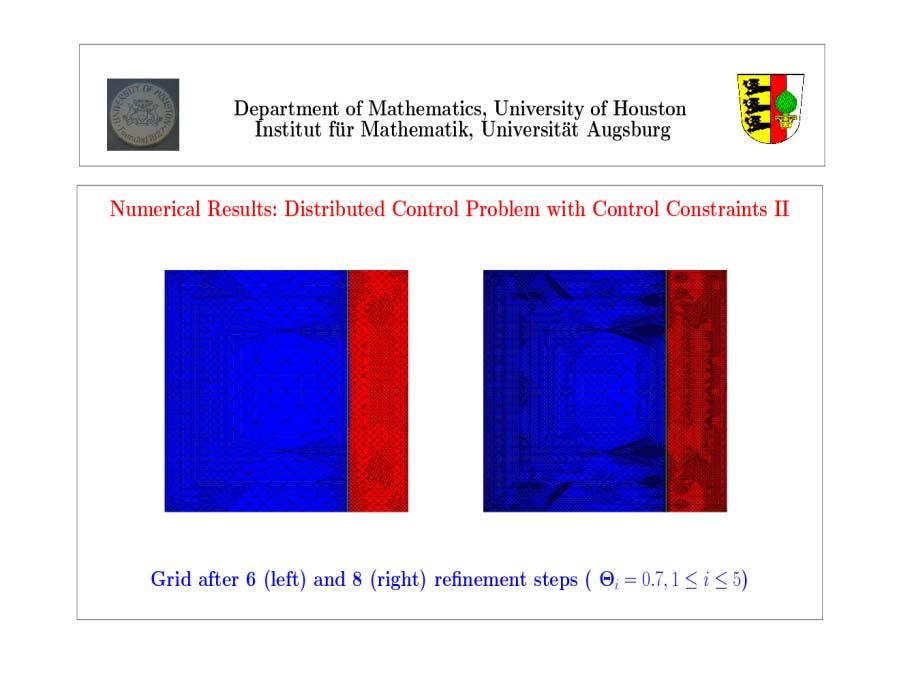
142 Numerical Results: Distributed Control Problem with Control Constraints II Grid after 6 (left) and 10 (right) refinement steps

143 Numerical Results: Distributed Control Problem with Control Constraints I l N dof δ h η h osc h ν h E E E E E E E E E E E E E E E E E E E E E E E E E E E E E E E E E E E E E E E E-16 Error (quantity of interest), estimator, oscillations, and consistency error

144 Numerical Results: Distributed Control Problem with Control Constraints II Decrease in the quantity of interest versus total number of DOFs

Basic Concepts of Adaptive Finite Element Methods for Elliptic Boundary Value Problems

Department of Mathematics, University of Houston Basic Concepts of Adaptive Finite Element Methods for Elliptic Boundary Value Problems Ronald H.W. Hoppe 1,2 1 Department of Mathematics, University of