Computing and Processing Correspondences with Functional Maps
|
|
|
- Toby Dorsey
- 5 years ago
- Views:
Transcription

1 Computing and Processing Correspondences with Functional Maps Maks Ovsjanikov 1 Etienne Corman 2 Michael Bronstein 3,4,5 Emanuele Rodolà 3 Mirela Ben-Chen 6 Leonidas Guibas 7 Frédéric Chazal 8 Alexander Bronstein 6,3,4 1 Ecole Polytechnique 3 USI Lugano 4 Tel Aviv University 5 Intel 2 CMU 6 Technion 7 Stanford University 8 INRIA SIGGRAPH Course, Los Angeles, 30 July /52
2 Functional Maps by Simultaneous Diagonalization of Laplacians 2/52


3 Choice of the basis Functional correspondence matrix C expressed in the Laplacian eigenbases Kovnatsky, Bronstein 2, Glashoff, Kimmel /52
4 Choice of the basis Functional correspondence matrix C expressed in the Laplacian eigenbases Kovnatsky, Bronstein 2, Glashoff, Kimmel /52
5 Problem with Laplacian eigenbases M φ M 2 φ M 3 φ M 4 φ M 5 φ M 6 N φ N 2 φ N 3 φ N 4 φ N 5 φ N 6 Kovnatsky, Bronstein 2, Glashoff, Kimmel /52
6 Problem with Laplacian eigenbases M φ M 2 φ M 3 φ M 4 φ M 5 φ M 6 N φ N 2 φ N 3 φ N 4 φ N 5 φ N 6 Isometric manifolds with simple spectrum: sign ambiguity T F φ M i = ±φ N i Kovnatsky, Bronstein 2, Glashoff, Kimmel /52
7 Problem with Laplacian eigenbases M φ M 2 φ M 3 φ M 4 φ M 5 φ M 6 N φ N 2 φ N 3 φ N 4 φ N 5 φ N 6 Isometric manifolds with simple spectrum: sign ambiguity T F φ M i = ±φ N i General spectrum: ambiguous rotation of eigenspace Kovnatsky, Bronstein 2, Glashoff, Kimmel /52
8 Problem with Laplacian eigenbases M φ M 2 φ M 3 φ M 4 φ M 5 φ M 6 N φ N 2 φ N 3 φ N 4 φ N 5 φ N 6 Isometric manifolds with simple spectrum: sign ambiguity T F φ M i = ±φ N i General spectrum: ambiguous rotation of eigenspace Non-isometric manifolds: eigenvectors can differ dramatically in order and form Kovnatsky, Bronstein 2, Glashoff, Kimmel /52

9 Problem with Laplacian eigenbases M φ M 2 φ M 3 φ M 4 φ M 5 φ M 6 N φ N 2 φ N 3 φ N 4 φ N 5 φ N 6 Isometric manifolds with simple spectrum: sign ambiguity T F φ M i = ±φ N i General spectrum: ambiguous rotation of eigenspace Non-isometric manifolds: eigenvectors can differ dramatically in order and form Incompatibilities tend to increase with frequency Kovnatsky, Bronstein 2, Glashoff, Kimmel /52
10 Coupled bases M a 1 +a 2 + +a k f φ M 1 φ M 2 φ M k T F N b 1 + b 2 + +b k g φ N 1 φ N 2 φ N k Kovnatsky, Bronstein 2, Glashoff, Kimmel /52
11 Coupled bases M a 1 +a 2 + +a k f T F φ M 1 φ M 2 φ M k a b N b 1 + b 2 + +b k g φ N 1 φ N 2 φ N k Kovnatsky, Bronstein 2, Glashoff, Kimmel /52
12 Coupled bases M â 1 +â 2 + +â k f ˆφ M 1 ˆφ M 2 ˆφ M k T F â ˆb N ˆb 1 + ˆb 2 + +ˆb k g ˆφ N 1 ˆφ N 2 ˆφ N k Kovnatsky, Bronstein 2, Glashoff, Kimmel /52
13 Coupled bases M â 1 +â 2 + +â k f ˆφ M 1 ˆφ M 2 ˆφ M k T F Ĉ I N ˆb 1 + ˆb 2 + +ˆb k g ˆφ N 1 ˆφ N 2 ˆφ N k Kovnatsky, Bronstein 2, Glashoff, Kimmel /52
14 Coupled bases Find a new pair of approximate orthonormal eigenbases ˆφ M i = p ji φ M j k ˆφ N i = q ji φ N j k j=1 j=1 parametrized by k k matrices P = (p ij ) and Q = (q ij ) i = 1,...,k Kovnatsky, Bronstein 2, Glashoff, Kimmel /52
15 Coupled bases Find a new pair of approximate orthonormal eigenbases ˆφ M i = p ji φ M j k ˆφ N i = q ji φ N j k j=1 j=1 parametrized by k k matrices P = (p ij ) and Q = (q ij ) i = 1,...,k Coupling: P A Q B Kovnatsky, Bronstein 2, Glashoff, Kimmel /52
16 Coupled bases Find a new pair of approximate orthonormal eigenbases ˆφ M i = p ji φ M j k ˆφ N i = q ji φ N j k j=1 j=1 parametrized by k k matrices P = (p ij ) and Q = (q ij ) i = 1,...,k Coupling: P A Q B Orthonormality: δ ij = ˆφ M i, ˆφ M j L2 (M) = k l,m=1 p li p mj φ M l,φ M m L2 (M) Kovnatsky, Bronstein 2, Glashoff, Kimmel /52
17 Coupled bases Find a new pair of approximate orthonormal eigenbases ˆφ M i = p ji φ M j k ˆφ N i = q ji φ N j k j=1 j=1 parametrized by k k matrices P = (p ij ) and Q = (q ij ) i = 1,...,k Coupling: P A Q B Orthonormality: δ ij = ˆφ M i, ˆφ M j L2 (M) = p li p lj k l=1 Kovnatsky, Bronstein 2, Glashoff, Kimmel /52
18 Coupled bases Find a new pair of approximate orthonormal eigenbases ˆφ M i = p ji φ M j k ˆφ N i = q ji φ N j k j=1 j=1 parametrized by k k matrices P = (p ij ) and Q = (q ij ) i = 1,...,k Coupling: P A Q B Orthonormality: δ ij = ˆφ M i, ˆφ M j L2 (M) = p li p lj = (P P) ij k l=1 Kovnatsky, Bronstein 2, Glashoff, Kimmel /52
19 Coupled bases Find a new pair of approximate orthonormal eigenbases ˆφ M i = p ji φ M j k ˆφ N i = q ji φ N j k j=1 j=1 parametrized by k k matrices P = (p ij ) and Q = (q ij ) i = 1,...,k Coupling: P A Q B Orthonormality: P P = I and Q Q = I Kovnatsky, Bronstein 2, Glashoff, Kimmel /52
20 Coupled bases Find a new pair of approximate orthonormal eigenbases ˆφ M i = p ji φ M j k ˆφ N i = q ji φ N j k j=1 j=1 parametrized by k k matrices P = (p ij ) and Q = (q ij ) i = 1,...,k Coupling: P A Q B Orthonormality: P P = I and Q Q = I Approximate eigenbasis: approximately diagonalizes the Laplacian ˆφ M i, ˆφ M j L2 (M) = k l,m=1 p li p mj φ M l, φ M m L2 (M) Kovnatsky, Bronstein 2, Glashoff, Kimmel /52
21 Coupled bases Find a new pair of approximate orthonormal eigenbases ˆφ M i = p ji φ M j k ˆφ N i = q ji φ N j k j=1 j=1 parametrized by k k matrices P = (p ij ) and Q = (q ij ) i = 1,...,k Coupling: P A Q B Orthonormality: P P = I and Q Q = I Approximate eigenbasis: approximately diagonalizes the Laplacian ˆφ M i, ˆφ M j L2 (M) = k l,m=1 p li p mj λ m φ M l,φ M m L2 (M) Kovnatsky, Bronstein 2, Glashoff, Kimmel /52
22 Coupled bases Find a new pair of approximate orthonormal eigenbases ˆφ M i = p ji φ M j k ˆφ N i = q ji φ N j k j=1 j=1 parametrized by k k matrices P = (p ij ) and Q = (q ij ) i = 1,...,k Coupling: P A Q B Orthonormality: P P = I and Q Q = I Approximate eigenbasis: approximately diagonalizes the Laplacian ˆφ M i, ˆφ M j L2 (M) = p li p lj λ l k l=1 Kovnatsky, Bronstein 2, Glashoff, Kimmel /52
23 Coupled bases Find a new pair of approximate orthonormal eigenbases ˆφ M i = p ji φ M j k ˆφ N i = q ji φ N j k j=1 j=1 parametrized by k k matrices P = (p ij ) and Q = (q ij ) i = 1,...,k Coupling: P A Q B Orthonormality: P P = I and Q Q = I Approximate eigenbasis: approximately diagonalizes the Laplacian ˆφ M i, ˆφ M j L2 (M) = p li p lj λ l = (P Λ M,k P) ij k l=1 Kovnatsky, Bronstein 2, Glashoff, Kimmel /52
24 Coupled bases Find a new pair of approximate orthonormal eigenbases ˆφ M i = p ji φ M j k ˆφ N i = q ji φ N j k j=1 j=1 parametrized by k k matrices P = (p ij ) and Q = (q ij ) i = 1,...,k Coupling: P A Q B Orthonormality: P P = I and Q Q = I Approximate eigenbasis: approximately diagonalizes the Laplacian ˆφ M i, ˆφ M j L2 (M) = p li p lj = (P Λ M,k P) ij 0, i j k l=1 Kovnatsky, Bronstein 2, Glashoff, Kimmel /52
25 Joint diagonalization problem min P,Q off(p Λ M,k P)+off(Q Λ N,k Q)+µ P A Q B s.t. P P = I Q Q = I Kovnatsky, Bronstein 2, Glashoff, Kimmel /52
26 Joint diagonalization problem min P,Q off(p Λ M,k P)+off(Q Λ N,k Q)+µ P A Q B s.t. P P = I Q Q = I Off-diagonal elements penalty off(x) = i j x2 ij Kovnatsky, Bronstein 2, Glashoff, Kimmel /52
27 Joint diagonalization problem min P,Q off(p Λ M,k P)+off(Q Λ N,k Q)+µ P A Q B s.t. P P = I Q Q = I Off-diagonal elements penalty off(x) = i j x2 ij Dirichlet energy off(x) = trace(x) for k > k Kovnatsky, Bronstein 2, Glashoff, Kimmel /52
28 Joint diagonalization problem min P,Q off(p Λ M,k P)+off(Q Λ N,k Q)+µ QP A B 2 F s.t. P P = I Q Q = I Off-diagonal elements penalty off(x) = i j x2 ij Dirichlet energy off(x) = trace(x) for k > k If Frobenius norm is used and k = k, due to rotation invariance C = QP is the functional correspondence matrix Kovnatsky, Bronstein 2, Glashoff, Kimmel /52
29 Joint diagonalization problem min P,Q off(p Λ M,k P)+off(Q Λ N,k Q)+µ P A Q B 2,1 s.t. P P = I Q Q = I Off-diagonal elements penalty off(x) = i j x2 ij Dirichlet energy off(x) = trace(x) for k > k If Frobenius norm is used and k = k, due to rotation invariance C = QP is the functional correspondence matrix Robust norm X 2,1 = j x j 2 allows coping with outliers Kovnatsky, Bronstein 2, Glashoff, Kimmel /52

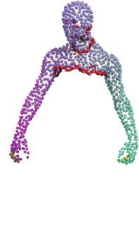
30 Example of joint diagonalization Mesh with 8.5K vertices Mesh with 850 vertices Kovnatsky, Bronstein 2, Glashoff, Kimmel /52
31 Example of joint diagonalization Mesh with 8.5K vertices Point cloud with 850 vertices Kovnatsky, Bronstein 2, Glashoff, Kimmel /52
32 Choice of the basis Functional correspondence matrix C expressed in standard Laplacian eigenbases Kovnatsky, Bronstein 2, Glashoff, Kimmel /52
33 Choice of the basis Functional correspondence matrix C expressed in coupled approximate eigenbases Kovnatsky, Bronstein 2, Glashoff, Kimmel /52
34 Multiple shapes C ij A i A j M j M i M p M 1 M 2 Kovnatsky, Bronstein 2, Glashoff, Kimmel 2013; Kovnatsky, Glashoff, Bronstein /52
35 Multiple shapes P i A i P j A j M j M i M p M 1 M 2 Kovnatsky, Bronstein 2, Glashoff, Kimmel 2013; Kovnatsky, Glashoff, Bronstein /52


36 Multiple shapes P i A i P j A j P j P i M j P p M i M p P 1 P 2 M 1 M 2 Kovnatsky, Bronstein 2, Glashoff, Kimmel 2013; Kovnatsky, Glashoff, Bronstein /52
37 Multiple shapes min P 1,...,P p p trace(p i Λ Mi P i )+µ P i A i P j A j i j i=1 s.t. P i P i = I Synchronization problem Matrices P 1,...,P p orthogonally align the p eigenbases Kovnatsky, Bronstein 2, Glashoff, Kimmel 2013; Kovnatsky, Glashoff, Bronstein /52
38 Computing Functional Maps with Manifold Optimization 13/52
39 min P trace(p ΛP)+µ PA B s.t. P P = I 14/52
40 min P trace(p ΛP)+µ PA B s.t. P P = I Optimization on the Stiefel manifold of orthogonal matrices 14/52
41 Manifold optimization toy example: eigenvalue problem min x R x Ax s.t. x x = 1 3 Minimization of a quadratic function on the sphere 15/52


42 Manifold optimization toy example: eigenvalue problem min x S(3,1) x Ax Minimization of a quadratic function on the sphere 15/52
43 Optimization on the manifold: main idea X (k) X (k+1) S Absil et al /52
44 Optimization on the manifold: main idea f(x (k) ) X (k) P X (k) S f(x (k) ) T X (k)s S Absil et al /52
45 Optimization on the manifold: main idea f(x (k) ) X (k) P X (k) α (k) S f(x (k) ) T X (k)s S Absil et al /52
 S f(x (k) ) T X (k)s R X (k) X (k+1) S Absil et al.")
46 Optimization on the manifold: main idea f(x (k) ) X (k) P X (k) α (k) S f(x (k) ) T X (k)s R X (k) X (k+1) S Absil et al /52
47 Optimization on the manifold repeat Compute extrinsic gradient f(x (k) ) Projection: S f(x (k) ) = P X (k)( f(x (k) )) Compute step size α (k) along the descent direction S f(x (k) ) Retraction: X (k+1) = R X (k)( α (k) S f(x (k) )) k k +1 until convergence; Absil et al. 2009; Boumal et al /52
48 Optimization on the manifold repeat Compute extrinsic gradient f(x (k) ) Projection: S f(x (k) ) = P X (k)( f(x (k) )) Compute step size α (k) along the descent direction S f(x (k) ) Retraction: X (k+1) = R X (k)( α (k) S f(x (k) )) k k +1 until convergence; Projection P and retraction R operators are manifold-dependent Absil et al. 2009; Boumal et al /52
49 Optimization on the manifold repeat Compute extrinsic gradient f(x (k) ) Projection: S f(x (k) ) = P X (k)( f(x (k) )) Compute step size α (k) along the descent direction S f(x (k) ) Retraction: X (k+1) = R X (k)( α (k) S f(x (k) )) k k +1 until convergence; Projection P and retraction R operators are manifold-dependent Typically expressed in closed form Absil et al. 2009; Boumal et al /52
50 Optimization on the manifold repeat Compute extrinsic gradient f(x (k) ) Projection: S f(x (k) ) = P X (k)( f(x (k) )) Compute step size α (k) along the descent direction S f(x (k) ) Retraction: X (k+1) = R X (k)( α (k) S f(x (k) )) k k +1 until convergence; Projection P and retraction R operators are manifold-dependent Typically expressed in closed form Black box : need to provide only f(x) and gradient f(x) Absil et al. 2009; Boumal et al /52
51 Partial Functional Maps 18/52
 Rodolà, Cosmo, Bronstein, Torsello, Cremers 2016")
52 Partial Laplacian eigenvectors ζ 2 ζ 3 ζ 4 ζ 5 ζ 6 ζ 7 ζ 8 ζ 9 ψ 2 ψ 3 ψ 4 ψ 5 ψ 6 ψ 7 ψ 8 ψ 9 φ 2 φ 3 φ 4 φ 5 φ 6 φ 7 φ 8 φ 9 Laplacian eigenvectors of a shape with missing parts (Neumann boundary conditions) Rodolà, Cosmo, Bronstein, Torsello, Cremers /52


53 Partial Laplacian eigenvectors Functional correspondence matrix C Rodolà, Cosmo, Bronstein, Torsello, Cremers /52
54 Perturbation analysis: intuition M M φ1 φ2 φ3 φ 1 φ 2 φ 3 λ 1 λ2 λ3 M λ 1 λ 2 λ 3 M M φ 1 φ 2 φ 3 M φ 1 φ2 φ3 λ 1 λ 1 λ 2 λ 3 λ2 λ3 Ignoring boundary interaction: disjoint parts (block-diagonal matrix) Eigenvectors = Mixture of eigenvectors of the parts Rodolà, Cosmo, Bronstein, Torsello, Cremers /52
 Consistent with Weyl s law")
55 Perturbation analysis: eigenvalues M r k N eigenvalue number Slope r k M N (depends on the area of the cut) Consistent with Weyl s law Rodolà, Cosmo, Bronstein, Torsello, Cremers /52

56 Perturbation analysis: details M M M M +td M te te M+tD M M Rodolà, Cosmo, Bronstein, Torsello, Cremers /52

 = i,j=1 j i λ i λ j Rodolà, Cosmo, Bronstein, Torsello, Cremers")
57 Perturbation analysis: boundary interaction strength 20 Value of f 10 Eigenvector perturbation depends on length and position of the boundary Perturbation strength c f(m)dm, where M n ( ) 2 φi (m)φ j (m) f(m) = i,j=1 j i λ i λ j Rodolà, Cosmo, Bronstein, Torsello, Cremers /52
58 Partial functional maps Model shape M Query shape N Part M M isometric to N Data f 1,...,f q L 2 (N) g 1,...,g q L 2 (M) Part M T F Query N Partial functional map (T F f i )(m) g i (m), m M Model M Rodolà, Cosmo, Bronstein, Torsello, Cremers /52
59 Partial functional maps Model shape M Query shape N Part M M isometric to N Data f 1,...,f q L 2 (N) g 1,...,g q L 2 (M) Part v T F Query N Partial functional map T F f i g i v, v : M [0,1] Model M Rodolà, Cosmo, Bronstein, Torsello, Cremers /52
60 Partial functional maps Model shape M Query shape N Part M M isometric to N Data f 1,...,f q L 2 (N) g 1,...,g q L 2 (M) Part v C Query N Partial functional map CA B(v), v : M [0,1] A = ( φ N ) i,f j L 2 (N) B(v) = ( φ M ) i,g j v L2 (M) Model M Rodolà, Cosmo, Bronstein, Torsello, Cremers /52
 Part v C Query N Partial functional map CA B(v), v : M [0,1] A = ( φ N ) i,f j L 2 (N) B(v) = ( φ M ) i,g j v L2 (M) Model M Optimization problem w.r.t. correspondence C and part v min C,v CA B(v) 2,1 +ρ corr (C)+ρ part (v) Rodolà, Cosmo, Bronstein, Torsello, Cremers 2016 25/52")
61 Partial functional maps Model shape M Query shape N Part M M isometric to N Data f 1,...,f q L 2 (N) g 1,...,g q L 2 (M) Part v C Query N Partial functional map CA B(v), v : M [0,1] A = ( φ N ) i,f j L 2 (N) B(v) = ( φ M ) i,g j v L2 (M) Model M Optimization problem w.r.t. correspondence C and part v min C,v CA B(v) 2,1 +ρ corr (C)+ρ part (v) Rodolà, Cosmo, Bronstein, Torsello, Cremers /52
62 Partial functional maps min CA B(v) 2,1 +ρ corr (C)+ρ part (v) C,v Rodolà, Cosmo, Bronstein, Torsello, Cremers /52
63 Partial functional maps min CA B(v) 2,1 +ρ corr (C)+ρ part (v) C,v Part regularization Area preservation v(m)dx N M Spatial regularity = small boundary length (Mumford-Shah) Rodolà, Cosmo, Bronstein, Torsello, Cremers 2016; Bronstein /52
64 Partial functional maps min CA B(v) 2,1 +ρ corr (C)+ρ part (v) C,v Part regularization Area preservation v(m)dx N M Spatial regularity = small boundary length (Mumford-Shah) Correspondence regularization Slanted diagonal structure Approximate ortho-projection (C C) i j 0 rank(c) r Rodolà, Cosmo, Bronstein, Torsello, Cremers 2016; Bronstein /52
65 Alternating minimization C-step: fix v, solve for correspondence C v-step: fix C, solve for part v min C CA B(v ) 2,1 +ρ corr (C) min v C A B(v) 2,1 +ρ part (v) Rodolà, Cosmo, Bronstein, Torsello, Cremers /52
 min v C A B(v) 2,1 +ρ part (v) Iteration 1 2 3 4 Rodolà, Cosmo, Bronstein, Torsello, Cremers 2016")
66 Alternating minimization C-step: fix v, solve for correspondence C v-step: fix C, solve for part v min C CA B(v ) 2,1 +ρ corr (C) min v C A B(v) 2,1 +ρ part (v) Iteration Rodolà, Cosmo, Bronstein, Torsello, Cremers /52
67 Example of convergence Time (sec.) C-step v-step Energy Iteration Rodolà, Cosmo, Bronstein, Torsello, Cremers /52


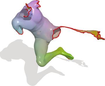
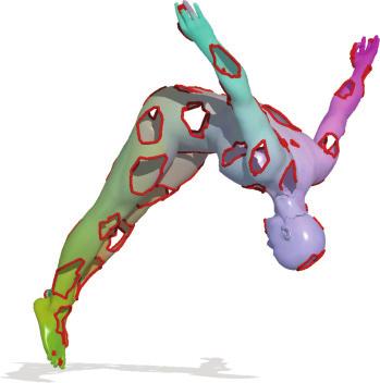

68 Examples of partial functional maps Rodolà, Cosmo, Bronstein, Torsello, Cremers /52


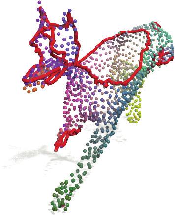


69 Examples of partial functional maps Rodolà, Cosmo, Bronstein, Torsello, Cremers /52


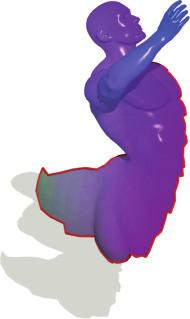

70 Examples of partial functional maps Rodolà, Cosmo, Bronstein, Torsello, Cremers /52


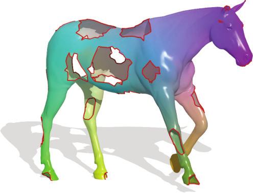

71 Examples of partial functional maps Rodolà, Cosmo, Bronstein, Torsello, Cremers /52
72 Partial functional maps vs Functional maps 100 % Correspondences PFM Func. maps Geodesic error Correspondence performance for different basis size k Rodolà, Cosmo, Bronstein, Torsello, Cremers /52
73 Partial correspondence performance 100 Cuts Holes % Correspondences Geodesic Error Geodesic Error PFM RF IM EN GT SHREC 16 Partial Matching benchmark Rodolà et al. 2016; Methods: Rodolà, Cosmo, Bronstein, Torsello, Cremers 2016 (PFM); Sahillioğlu, Yemez 2012 (IM); Rodolà, Bronstein, Albarelli, Bergamasco, Torsello 2012 (GT); Rodolà et al (EN); Rodolà et al (RF) 31/52
74 Partial correspondence performance 1 Cuts Holes Mean geodesic error Partiality (%) Partiality (%) PFM RF IM EN GT SHREC 16 Partial Matching benchmark Rodolà et al. 2016; Methods: Rodolà, Cosmo, Bronstein, Torsello, Cremers 2016 (PFM); Sahillioğlu, Yemez 2012 (IM); Rodolà, Bronstein, Albarelli, Bergamasco, Torsello 2012 (GT); Rodolà et al (EN); Rodolà et al (RF) 32/52

75 Partial correspondence (part-to-full) Rodolà, Cosmo, Bronstein, Torsello, Cremers /52
76 Partial correspondence (part-to-part) Litany, Rodolà, Bronstein 2, Cremers /52
77 Key observation M N N C NN slant N N M C MM slant M M Litany, Rodolà, Bronstein 2, Cremers /52
78 Key observation M N N M C NM = C MM C NM C NN slant N M N M Litany, Rodolà, Bronstein 2, Cremers /52
79 Key observation M N N M Litany, Rodolà, Bronstein 2, Cremers 2016 C NM = C MM C NM C NN slant N M N M = M N 34/52

80 Partial correspondence (part-to-part) Litany, Rodolà, Bronstein 2, Cremers /52

81 Non-rigid puzzle (multi-part) Litany, Rodolà, Bronstein 2, Cremers /52

82 Litany, Bronstein
83 Non-rigid puzzles problem formulation Input Model M Parts N 1,...,N p Output Segmentation M i M Located parts N i N i Clutter Ni c Missing parts M 0 M 1 M 2 M 0 T F1 N N c 1 T 2 F2 N1 c N 2 Part N 1 Correspondences T Fi Model M Part N 2 Litany, Rodolà, Bronstein 2, Cremers /52

84 Non-rigid puzzles problem formulation Input Model M Parts N 1,...,N p Output Segmentation u i :M [0,1] Located parts v i :N i [0,1] Clutter 1 v i Missing parts u 0 u 1 u 2 u 0 C 1 C 2 v 2 v 1 Part N 1 Correspondences C i Model M Part N 2 Litany, Rodolà, Bronstein 2, Cremers /52
85 Non-rigid puzzles problem formulation min C i,u i,v i s.t. p p p C i A i (v i ) B(u i ) 2,1 + ρ part (u i,v i )+ ρ corr (C i ) i=1 p u i = 1 i=0 i=0 i=1 Litany, Rodolà, Bronstein 2, Cremers /52
86 Convergence example Outer iteration 1 Litany, Rodolà, Bronstein 2, Cremers /52
87 Convergence example Outer iteration 2 Litany, Rodolà, Bronstein 2, Cremers /52

88 Convergence example Outer iteration 3 Litany, Rodolà, Bronstein 2, Cremers /52
89 Convergence example Time (sec) Iteration number Litany, Rodolà, Bronstein 2, Cremers /52
90 Example: Perfect puzzle Model/Part Synthetic (TOSCA) Transformation Isometric Clutter No Missing part No Data term Dense (SHOT) Litany, Rodolà, Bronstein 2, Cremers /52
 Segmentation Litany, Rodolà, Bronstein 2, Cremers 2016")
91 Example: Perfect puzzle Model/Part Synthetic (TOSCA) Transformation Isometric Clutter No Missing part No Data term Dense (SHOT) Segmentation Litany, Rodolà, Bronstein 2, Cremers /52
92 Example: Perfect puzzle Model/Part Synthetic (TOSCA) Transformation Isometric Clutter No Missing part No Data term Dense (SHOT) Correspondence Litany, Rodolà, Bronstein 2, Cremers /52
93 Example: Overlapping parts Model/Part Synthetic (FAUST) Transformation Near-isometric Clutter Yes (overlap) Missing part No Data term Dense (SHOT) Segmentation Litany, Rodolà, Bronstein 2, Cremers /52
94 Example: Overlapping parts Model/Part Synthetic (FAUST) Transformation Near-isometric Clutter Yes (overlap) Missing part No Data term Dense (SHOT) Correspondence Litany, Rodolà, Bronstein 2, Cremers /52
95 Example: Missing parts Model/Part Synthetic (TOSCA) Transformation Isometric Clutter Yes (extra part) Missing part Yes Data term Dense (SHOT) Litany, Rodolà, Bronstein 2, Cremers /52
96 Example: Missing parts Model/Part Synthetic (TOSCA) Transformation Isometric Clutter Yes (extra part) Missing part Yes Data term Dense (SHOT) Litany, Rodolà, Bronstein 2, Cremers 2016 Segmentation 43/52
97 Example: Missing parts Model/Part Synthetic (TOSCA) Transformation Isometric Clutter Yes (extra part) Missing part Yes Data term Dense (SHOT) Litany, Rodolà, Bronstein 2, Cremers 2016 Correspondence 43/52
98 Partial functional correspondence with spatial part model M φ M 1 φ M 2 φ M 3 φ M 4 φ M 5 φ M 6 T F N N φ N 1 φ N 2 φ N 3 φ N 4 φ N 5 φ N 6 Slanted diagonal: T F φ M i,v φ N j L 2 (N) ±δ i,πj Complicated alternating optimization w.r.t. v and C Explicit spatial model v of the part O(n) complexity! Litany, Rodolà, Bronstein π j j N M 44/52
99 Spectral partial functional correspondence M φ M 1 φ M 2 φ M 3 φ M 4 φ M 5 φ M 6 T F N ˆφ N 1 ˆφ N 2 ˆφ N 3 ˆφ N 4 ˆφ N 5 ˆφ N 6 Find a new basis {ˆφ N i }k i=1 such that T Fφ M i, ˆφ N j L 2 (N) δ ij Litany, Rodolà, Bronstein /52
100 Spectral partial functional correspondence M φ M 1 φ M 2 φ M 3 φ M 4 φ M 5 φ M 6 T F N ˆφ N 1 ˆφ N 2 ˆφ N 3 ˆφ N 4 ˆφ N 5 ˆφ N 6 Find a new basis {ˆφ N i }k i=1 such that T Fφ M i, k l=1 q ljφ N l L 2 (N) δ ij New basis functions {ˆφ N i }k i=1 are localized on N Optimization over coefficients Q = (q ij ) O(k 2 ) complexity! Litany, Rodolà, Bronstein /52
101 Spectral partial functional correspondence A k q Π k k B k q Litany, Rodolà, Bronstein /52
102 Spectral partial functional correspondence A r q Πr k B k q Π is k r partial permutation with elements (π i,i) = ±1 and r k M N Litany, Rodolà, Bronstein /52
103 Spectral partial functional correspondence A r q Πr k B k q Π is k r partial permutation with elements (π i,i) = ±1 and r k M N Relax Π Q s.t. Q Q = I (k r ortho-projection) min Q trace(q Λ N,k Q)+µ A r Q B k 2,1 s.t. Q Q = I Litany, Rodolà, Bronstein ; Kovnatsky, Glashoff, Bronstein 2, Kimmel 2013 (Joint diag) 46/52
104 Spectral partial functional correspondence A r q Πr k B k q Π is k r partial permutation with elements (π i,i) = ±1 and r k M N Relax Π Q s.t. Q Q = I (k r ortho-projection) min Q trace(q Λ N,k Q)+µ A r Q B k 2,1 s.t. Q Q = I Optimization on the Stiefel manifold with k 2 variables Litany, Rodolà, Bronstein ; Kovnatsky, Glashoff, Bronstein 2, Kimmel 2013 (Joint diag) 46/52
105 Spectral partial functional correspondence A r q Πr k B k q Π is k r partial permutation with elements (π i,i) = ±1 and r k M N Relax Π Q s.t. Q Q = I (k r ortho-projection) min Q trace(q Λ N,k Q)+µ A r Q B k 2,1 s.t. Q Q = I Non-smooth optimization on the Stiefel manifold with k 2 variables Litany, Rodolà, Bronstein ; Kovnatsky, Glashoff, Bronstein 2, Kimmel 2013 (Joint diag); Kovnatsky, Glashoff, Bronstein 2016 (MADMM) 46/52
106 Spectral partial functional correspondence A r q Πr k B k q Π is k r partial permutation with elements (π i,i) = ±1 and r k M N Relax Π Q s.t. Q Q = I (k r ortho-projection) min Q trace(q Λ N,k Q)+µ A r Q B k 2,1 s.t. Q Q = I Non-smooth optimization on the Stiefel manifold with k 2 variables Non-rigid alignment of eigenfunctions Litany, Rodolà, Bronstein ; Kovnatsky, Glashoff, Bronstein 2, Kimmel 2013 (Joint diag); Kovnatsky, Glashoff, Bronstein 2016 (MADMM) 46/52


107 Geometric interpretation Full shape N φ M 2,φM 3 and φ N 2,φN 3 Laplacian eigenbasis Part M φ M 2,φM 3 and ˆφ N 2, ˆφ N 3 New basis Litany, Rodolà, Bronstein /52


108 Convergence example Initialization Litany, Rodolà, Bronstein /52


109 Increasing partiality SPFM PFM rank = 36 rank = 23 rank = 7 Litany, Rodolà, Bronstein /52
110 SHREC 16 Partiality 100 cuts holes % Correspondences Geodesic Error Geodesic Error SPFM JAD RF PFM IM EN GT SHREC 16 Partial Matching benchmark: Rodolà et al. 2016; Methods: Unpublished work (SPFM); Rodolà, Cosmo, Bronstein, Torsello, Cremers 2016 (PFM); Sahillioğlu, Yemez 2012 (IM); Rodolà, Bronstein, Albarelli, Bergamasco, Torsello 2012 (GT); Rodolà et al (EN); Rodolà et al (RF) 50/52
111 Runtime Mean time per iteration (sec) SPFM PFM Number of vertices ( 10 4 ) Litany, Rodolà, Bronstein /52

112 Correspondence examples: topological noise Litany, Rodolà, Bronstein ; data: Bogo et al (FAUST) 52/52

113 Correspondence examples: topological noise Litany, Rodolà, Bronstein ; data: Bogo et al (FAUST) 52/52

114 Correspondence examples: topological noise Litany, Rodolà, Bronstein ; data: Rodola et al (SHREC) 52/52

115 Correspondence examples: topological noise Litany, Rodolà, Bronstein ; data: Rodola et al (SHREC) 52/52
Linear Algebra: Matrix Eigenvalue Problems
 CHAPTER8 Linear Algebra: Matrix Eigenvalue Problems Chapter 8 p1 A matrix eigenvalue problem considers the vector equation (1) Ax = λx. 8.0 Linear Algebra: Matrix Eigenvalue Problems Here A is a given
Functional Maps ( ) Dr. Emanuele Rodolà Room , Informatik IX
 Dr. Emanuele Rodolà Room , Informatik IX") Functional Maps (12.06.2014) Dr. Emanuele Rodolà rodola@in.tum.de Room 02.09.058, Informatik IX Seminar «LP relaxation for elastic shape matching» Fabian Stark Wednesday, June 18th 14:00 Room 02.09.023
Functional Maps (12.06.2014) Dr. Emanuele Rodolà rodola@in.tum.de Room 02.09.058, Informatik IX Seminar «LP relaxation for elastic shape matching» Fabian Stark Wednesday, June 18th 14:00 Room 02.09.023
Graph Matching: Relax or Not? Alex Bronstein. Simons Institute, Berkeley, Joint work with Yonathan Aflalo and Ron Kimmel
 Graph Matching: Relax or Not? Alex Bronstein School of Electrical Engineering Tel Aviv University College of Electrical and Computer Engineering Duke University Simons Institute, Berkeley, 2014 Joint work
Functional Analysis Review
 Outline 9.520: Statistical Learning Theory and Applications February 8, 2010 Outline 1 2 3 4 Vector Space Outline A vector space is a set V with binary operations +: V V V and : R V V such that for all
Lift me up but not too high Fast algorithms to solve SDP s with block-diagonal constraints
 Lift me up but not too high Fast algorithms to solve SDP s with block-diagonal constraints Nicolas Boumal Université catholique de Louvain (Belgium) IDeAS seminar, May 13 th, 2014, Princeton The Riemannian
Stable Spectral Mesh Filtering
 Stable Spectral Mesh Filtering Artiom Kovnatsky, Michael M. Bronstein, and Alexander M. Bronstein 2 Institute of Computational Science, Faculty of Informatics, Università della Svizzera Italiana, Lugano,
The Laplacian ( ) Matthias Vestner Dr. Emanuele Rodolà Room , Informatik IX
 Matthias Vestner Dr. Emanuele Rodolà Room , Informatik IX") The Laplacian (26.05.2014) Matthias Vestner Dr. Emanuele Rodolà {vestner,rodola}@in.tum.de Room 02.09.058, Informatik IX Seminar «The metric approach to shape matching» Alfonso Ros Wednesday, May 28th
The Laplacian (26.05.2014) Matthias Vestner Dr. Emanuele Rodolà {vestner,rodola}@in.tum.de Room 02.09.058, Informatik IX Seminar «The metric approach to shape matching» Alfonso Ros Wednesday, May 28th
1 Inner Product and Orthogonality
 CSCI 4/Fall 6/Vora/GWU/Orthogonality and Norms Inner Product and Orthogonality Definition : The inner product of two vectors x and y, x x x =.., y =. x n y y... y n is denoted x, y : Note that n x, y =
Justin Solomon MIT, Spring 2017
 Justin Solomon MIT, Spring 2017 http://pngimg.com/upload/hammer_png3886.png You can learn a lot about a shape by hitting it (lightly) with a hammer! What can you learn about its shape from vibration frequencies
Spectral Algorithms I. Slides based on Spectral Mesh Processing Siggraph 2010 course
 Spectral Algorithms I Slides based on Spectral Mesh Processing Siggraph 2010 course Why Spectral? A different way to look at functions on a domain Why Spectral? Better representations lead to simpler solutions
6/9/2010. Feature-based methods and shape retrieval problems. Structure. Combining local and global structures. Photometric stress
 1 2 Structure Feature-based methods and shape retrieval problems Global Metric Local Feature descriptors Alexander & Michael Bronstein, 2006-2009 Michael Bronstein, 2010 tosca.cs.technion.ac.il/book 048921
Chapter 7: Symmetric Matrices and Quadratic Forms
 Chapter 7: Symmetric Matrices and Quadratic Forms (Last Updated: December, 06) These notes are derived primarily from Linear Algebra and its applications by David Lay (4ed). A few theorems have been moved
CALCULUS ON MANIFOLDS. 1. Riemannian manifolds Recall that for any smooth manifold M, dim M = n, the union T M =
 CALCULUS ON MANIFOLDS 1. Riemannian manifolds Recall that for any smooth manifold M, dim M = n, the union T M = a M T am, called the tangent bundle, is itself a smooth manifold, dim T M = 2n. Example 1.
IFT LAPLACIAN APPLICATIONS. Mikhail Bessmeltsev
 IFT 6112 09 LAPLACIAN APPLICATIONS http://www-labs.iro.umontreal.ca/~bmpix/teaching/6112/2018/ Mikhail Bessmeltsev Rough Intuition http://pngimg.com/upload/hammer_png3886.png You can learn a lot about
Finding normalized and modularity cuts by spectral clustering. Ljubjana 2010, October
 Finding normalized and modularity cuts by spectral clustering Marianna Bolla Institute of Mathematics Budapest University of Technology and Economics marib@math.bme.hu Ljubjana 2010, October Outline Find
Second-Order Inference for Gaussian Random Curves
 Second-Order Inference for Gaussian Random Curves With Application to DNA Minicircles Victor Panaretos David Kraus John Maddocks Ecole Polytechnique Fédérale de Lausanne Panaretos, Kraus, Maddocks (EPFL)
Lecture 10: Dimension Reduction Techniques
 Lecture 10: Dimension Reduction Techniques Radu Balan Department of Mathematics, AMSC, CSCAMM and NWC University of Maryland, College Park, MD April 17, 2018 Input Data It is assumed that there is a set
On the optimality of shape and data representation in the spectral domain
 On the optimality of shape and data representation in the spectral domain Yonathan Aflalo Haim Brezis Ron Kimmel arxiv:1409.4349v1 [cs.cv] 15 Sep 014 October 11, 018 Abstract A proof of the optimality
Lecture 5 : Projections
 Lecture 5 : Projections EE227C. Lecturer: Professor Martin Wainwright. Scribe: Alvin Wan Up until now, we have seen convergence rates of unconstrained gradient descent. Now, we consider a constrained minimization
Heat Kernel Signature: A Concise Signature Based on Heat Diffusion. Leo Guibas, Jian Sun, Maks Ovsjanikov
 Heat Kernel Signature: A Concise Signature Based on Heat Diffusion i Leo Guibas, Jian Sun, Maks Ovsjanikov This talk is based on: Jian Sun, Maks Ovsjanikov, Leonidas Guibas 1 A Concise and Provably Informative
APPROXIMATELY ISOMETRIC SHAPE CORRESPONDENCE BY MATCHING POINTWISE SPECTRAL FEATURES AND GLOBAL GEODESIC STRUCTURES
 Advances in Adaptive Data Analysis Vol. 3, Nos. 1 & 2 (2011) 203 228 c World Scientific Publishing Company DOI: 10.1142/S1793536911000829 APPROXIMATELY ISOMETRIC SHAPE CORRESPONDENCE BY MATCHING POINTWISE
Exercise Set 7.2. Skills
 Orthogonally diagonalizable matrix Spectral decomposition (or eigenvalue decomposition) Schur decomposition Subdiagonal Upper Hessenburg form Upper Hessenburg decomposition Skills Be able to recognize
a 11 a 12 a 11 a 12 a 13 a 21 a 22 a 23 . a 31 a 32 a 33 a 12 a 21 a 23 a 31 a = = = = 12
 24 8 Matrices Determinant of 2 2 matrix Given a 2 2 matrix [ ] a a A = 2 a 2 a 22 the real number a a 22 a 2 a 2 is determinant and denoted by det(a) = a a 2 a 2 a 22 Example 8 Find determinant of 2 2
Spectral Processing. Misha Kazhdan
 Spectral Processing Misha Kazhdan [Taubin, 1995] A Signal Processing Approach to Fair Surface Design [Desbrun, et al., 1999] Implicit Fairing of Arbitrary Meshes [Vallet and Levy, 2008] Spectral Geometry
Spectral Algorithms II
 Spectral Algorithms II Applications Slides based on Spectral Mesh Processing Siggraph 2010 course Applications Shape retrieval Parameterization i 1D 2D Quad meshing Shape Retrieval 3D Repository Query
LECTURE NOTE #11 PROF. ALAN YUILLE
 LECTURE NOTE #11 PROF. ALAN YUILLE 1. NonLinear Dimension Reduction Spectral Methods. The basic idea is to assume that the data lies on a manifold/surface in D-dimensional space, see figure (1) Perform
CS 468, Spring 2013 Differential Geometry for Computer Science Justin Solomon and Adrian Butscher
 CS 468, Spring 2013 Differential Geometry for Computer Science Justin Solomon and Adrian Butscher http://graphics.stanford.edu/projects/lgl/papers/nbwyg-oaicsm-11/nbwyg-oaicsm-11.pdf Need to understand
EE Technion, Spring then. can be isometrically embedded into can be realized as a Gram matrix of rank, Properties:
 5/25/200 2 A mathematical exercise Assume points with the metric are isometrically embeddable into Then, there exists a canonical form such that for all Spectral methods We can also write Alexander & Michael
The University of Texas at Austin Department of Electrical and Computer Engineering. EE381V: Large Scale Learning Spring 2013.
 The University of Texas at Austin Department of Electrical and Computer Engineering EE381V: Large Scale Learning Spring 2013 Assignment Two Caramanis/Sanghavi Due: Tuesday, Feb. 19, 2013. Computational
Data Analysis and Manifold Learning Lecture 9: Diffusion on Manifolds and on Graphs
 Data Analysis and Manifold Learning Lecture 9: Diffusion on Manifolds and on Graphs Radu Horaud INRIA Grenoble Rhone-Alpes, France Radu.Horaud@inrialpes.fr http://perception.inrialpes.fr/ Outline of Lecture
Spectral clustering. Two ideal clusters, with two points each. Spectral clustering algorithms
 A simple example Two ideal clusters, with two points each Spectral clustering Lecture 2 Spectral clustering algorithms 4 2 3 A = Ideally permuted Ideal affinities 2 Indicator vectors Each cluster has an
Lecture 3: Latent Variables Models and Learning with the EM Algorithm. Sam Roweis. Tuesday July25, 2006 Machine Learning Summer School, Taiwan
 Lecture 3: Latent Variables Models and Learning with the EM Algorithm Sam Roweis Tuesday July25, 2006 Machine Learning Summer School, Taiwan Latent Variable Models What to do when a variable z is always
The Projected Power Method: An Efficient Algorithm for Joint Alignment from Pairwise Differences
 The Projected Power Method: An Efficient Algorithm for Joint Alignment from Pairwise Differences Yuxin Chen Emmanuel Candès Department of Statistics, Stanford University, Sep. 2016 Nonconvex optimization
Synopsis of Numerical Linear Algebra
 Synopsis of Numerical Linear Algebra Eric de Sturler Department of Mathematics, Virginia Tech sturler@vt.edu http://www.math.vt.edu/people/sturler Iterative Methods for Linear Systems: Basics to Research
Compression, Matrix Range and Completely Positive Map
 Compression, Matrix Range and Completely Positive Map Iowa State University Iowa-Nebraska Functional Analysis Seminar November 5, 2016 Definitions and notations H, K : Hilbert space. If dim H = n
EE/ACM Applications of Convex Optimization in Signal Processing and Communications Lecture 17
 EE/ACM 150 - Applications of Convex Optimization in Signal Processing and Communications Lecture 17 Andre Tkacenko Signal Processing Research Group Jet Propulsion Laboratory May 29, 2012 Andre Tkacenko
CS281 Section 4: Factor Analysis and PCA
 CS81 Section 4: Factor Analysis and PCA Scott Linderman At this point we have seen a variety of machine learning models, with a particular emphasis on models for supervised learning. In particular, we
arxiv: v1 [math.oc] 22 May 2018
![arxiv: v1 [math.oc] 22 May 2018](/thumbs/92/110287813.jpg "arxiv: v1 [math.oc] 22 May 2018") On the Connection Between Sequential Quadratic Programming and Riemannian Gradient Methods Yu Bai Song Mei arxiv:1805.08756v1 [math.oc] 22 May 2018 May 23, 2018 Abstract We prove that a simple Sequential
On the Connection Between Sequential Quadratic Programming and Riemannian Gradient Methods Yu Bai Song Mei arxiv:1805.08756v1 [math.oc] 22 May 2018 May 23, 2018 Abstract We prove that a simple Sequential
Matrix stabilization using differential equations.
 Matrix stabilization using differential equations. Nicola Guglielmi Universitá dell Aquila and Gran Sasso Science Institute, Italia NUMOC-2017 Roma, 19 23 June, 2017 Inspired by a joint work with Christian
Basic Calculus Review
 Basic Calculus Review Lorenzo Rosasco ISML Mod. 2 - Machine Learning Vector Spaces Functionals and Operators (Matrices) Vector Space A vector space is a set V with binary operations +: V V V and : R V
E2 212: Matrix Theory (Fall 2010) Solutions to Test - 1
 Solutions to Test - 1") E2 212: Matrix Theory (Fall 2010) s to Test - 1 1. Let X = [x 1, x 2,..., x n ] R m n be a tall matrix. Let S R(X), and let P be an orthogonal projector onto S. (a) If X is full rank, show that P can be
E2 212: Matrix Theory (Fall 2010) s to Test - 1 1. Let X = [x 1, x 2,..., x n ] R m n be a tall matrix. Let S R(X), and let P be an orthogonal projector onto S. (a) If X is full rank, show that P can be
235 Final exam review questions
 5 Final exam review questions Paul Hacking December 4, 0 () Let A be an n n matrix and T : R n R n, T (x) = Ax the linear transformation with matrix A. What does it mean to say that a vector v R n is an
Conjugate Gradient Method
 Conjugate Gradient Method direct and indirect methods positive definite linear systems Krylov sequence spectral analysis of Krylov sequence preconditioning Prof. S. Boyd, EE364b, Stanford University Three
arxiv: v1 [cs.gr] 16 Oct 2013
![arxiv: v1 [cs.gr] 16 Oct 2013](/thumbs/74/70918581.jpg "arxiv: v1 [cs.gr] 16 Oct 2013") MATCHING LBO EIGENSPACE OF NON-RIGID SHAPES VIA HIGH ORDER STATISTICS Alon Shtern, Ron Kimmel arxiv:1310.4459v1 [cs.gr] 16 Oct 2013 Technion - Israel Institute of Technology Abstract A fundamental tool
MATCHING LBO EIGENSPACE OF NON-RIGID SHAPES VIA HIGH ORDER STATISTICS Alon Shtern, Ron Kimmel arxiv:1310.4459v1 [cs.gr] 16 Oct 2013 Technion - Israel Institute of Technology Abstract A fundamental tool
Jordan normal form notes (version date: 11/21/07)
") Jordan normal form notes (version date: /2/7) If A has an eigenbasis {u,, u n }, ie a basis made up of eigenvectors, so that Au j = λ j u j, then A is diagonal with respect to that basis To see this, let
Jordan normal form notes (version date: /2/7) If A has an eigenbasis {u,, u n }, ie a basis made up of eigenvectors, so that Au j = λ j u j, then A is diagonal with respect to that basis To see this, let
Laplace-Beltrami Eigenfunctions for Deformation Invariant Shape Representation
 Laplace-Beltrami Eigenfunctions for Deformation Invariant Shape Representation Author: Raif M. Rustamov Presenter: Dan Abretske Johns Hopkins 2007 Outline Motivation and Background Laplace-Beltrami Operator
APPENDIX A. Background Mathematics. A.1 Linear Algebra. Vector algebra. Let x denote the n-dimensional column vector with components x 1 x 2.
 APPENDIX A Background Mathematics A. Linear Algebra A.. Vector algebra Let x denote the n-dimensional column vector with components 0 x x 2 B C @. A x n Definition 6 (scalar product). The scalar product
Linear Algebra in Computer Vision. Lecture2: Basic Linear Algebra & Probability. Vector. Vector Operations
 Linear Algebra in Computer Vision CSED441:Introduction to Computer Vision (2017F Lecture2: Basic Linear Algebra & Probability Bohyung Han CSE, POSTECH bhhan@postech.ac.kr Mathematics in vector space Linear
EXERCISES ON DETERMINANTS, EIGENVALUES AND EIGENVECTORS. 1. Determinants
 EXERCISES ON DETERMINANTS, EIGENVALUES AND EIGENVECTORS. Determinants Ex... Let A = 0 4 4 2 0 and B = 0 3 0. (a) Compute 0 0 0 0 A. (b) Compute det(2a 2 B), det(4a + B), det(2(a 3 B 2 )). 0 t Ex..2. For
arxiv: v1 [cs.cv] 28 Sep 2012
![arxiv: v1 [cs.cv] 28 Sep 2012](/thumbs/87/96944851.jpg "arxiv: v1 [cs.cv] 28 Sep 2012") Coupled quasi-harmonic bases arxiv:1210.0026v1 [cs.cv] 28 Sep 2012 A. Kovnatsky 1, M. M. Bronstein 1, A. M. Bronstein 2, K. Glashoff 3, and R. Kimmel 4 1 Faculty of Informatics, Università della Svizzera
Coupled quasi-harmonic bases arxiv:1210.0026v1 [cs.cv] 28 Sep 2012 A. Kovnatsky 1, M. M. Bronstein 1, A. M. Bronstein 2, K. Glashoff 3, and R. Kimmel 4 1 Faculty of Informatics, Università della Svizzera
Lectures in Discrete Differential Geometry 2 Surfaces
 Lectures in Discrete Differential Geometry 2 Surfaces Etienne Vouga February 4, 24 Smooth Surfaces in R 3 In this section we will review some properties of smooth surfaces R 3. We will assume that is parameterized
Graphs, Geometry and Semi-supervised Learning
 Graphs, Geometry and Semi-supervised Learning Mikhail Belkin The Ohio State University, Dept of Computer Science and Engineering and Dept of Statistics Collaborators: Partha Niyogi, Vikas Sindhwani In
Review of similarity transformation and Singular Value Decomposition
 Review of similarity transformation and Singular Value Decomposition Nasser M Abbasi Applied Mathematics Department, California State University, Fullerton July 8 7 page compiled on June 9, 5 at 9:5pm
Singular Value Decomposition
 Singular Value Decomposition CS 205A: Mathematical Methods for Robotics, Vision, and Graphics Doug James (and Justin Solomon) CS 205A: Mathematical Methods Singular Value Decomposition 1 / 35 Understanding
Statistical Pattern Recognition
 Statistical Pattern Recognition Feature Extraction Hamid R. Rabiee Jafar Muhammadi, Alireza Ghasemi, Payam Siyari Spring 2014 http://ce.sharif.edu/courses/92-93/2/ce725-2/ Agenda Dimensionality Reduction
Basic Math for
 Basic Math for 16-720 August 23, 2002 1 Linear Algebra 1.1 Vectors and Matrices First, a reminder of a few basic notations, definitions, and terminology: Unless indicated otherwise, vectors are always
ICS 6N Computational Linear Algebra Symmetric Matrices and Orthogonal Diagonalization
 ICS 6N Computational Linear Algebra Symmetric Matrices and Orthogonal Diagonalization Xiaohui Xie University of California, Irvine xhx@uci.edu Xiaohui Xie (UCI) ICS 6N 1 / 21 Symmetric matrices An n n
Graph Partitioning Using Random Walks
 Graph Partitioning Using Random Walks A Convex Optimization Perspective Lorenzo Orecchia Computer Science Why Spectral Algorithms for Graph Problems in practice? Simple to implement Can exploit very efficient
1 Last time: least-squares problems
 MATH Linear algebra (Fall 07) Lecture Last time: least-squares problems Definition. If A is an m n matrix and b R m, then a least-squares solution to the linear system Ax = b is a vector x R n such that
SPECTRAL THEOREM FOR COMPACT SELF-ADJOINT OPERATORS
 SPECTRAL THEOREM FOR COMPACT SELF-ADJOINT OPERATORS G. RAMESH Contents Introduction 1 1. Bounded Operators 1 1.3. Examples 3 2. Compact Operators 5 2.1. Properties 6 3. The Spectral Theorem 9 3.3. Self-adjoint
Econ 204 Supplement to Section 3.6 Diagonalization and Quadratic Forms. 1 Diagonalization and Change of Basis
 Econ 204 Supplement to Section 3.6 Diagonalization and Quadratic Forms De La Fuente notes that, if an n n matrix has n distinct eigenvalues, it can be diagonalized. In this supplement, we will provide
14 Singular Value Decomposition
 14 Singular Value Decomposition For any high-dimensional data analysis, one s first thought should often be: can I use an SVD? The singular value decomposition is an invaluable analysis tool for dealing
Definition and basic properties of heat kernels I, An introduction
 Definition and basic properties of heat kernels I, An introduction Zhiqin Lu, Department of Mathematics, UC Irvine, Irvine CA 92697 April 23, 2010 In this lecture, we will answer the following questions:
Spectral Graph Theory and its Applications. Daniel A. Spielman Dept. of Computer Science Program in Applied Mathematics Yale Unviersity
 Spectral Graph Theory and its Applications Daniel A. Spielman Dept. of Computer Science Program in Applied Mathematics Yale Unviersity Outline Adjacency matrix and Laplacian Intuition, spectral graph drawing
Synchronization over Cartan motion groups via contraction
 Synchronization over Cartan motion groups via contraction Onur Özyeşil, Nir Sharon 1, and Amit Singer 1, 1 Program in Applied and Computational Mathematics, Princeton University Department of Mathematics,
Data Analysis and Manifold Learning Lecture 3: Graphs, Graph Matrices, and Graph Embeddings
 Data Analysis and Manifold Learning Lecture 3: Graphs, Graph Matrices, and Graph Embeddings Radu Horaud INRIA Grenoble Rhone-Alpes, France Radu.Horaud@inrialpes.fr http://perception.inrialpes.fr/ Outline
Noisy Streaming PCA. Noting g t = x t x t, rearranging and dividing both sides by 2η we get
 Supplementary Material A. Auxillary Lemmas Lemma A. Lemma. Shalev-Shwartz & Ben-David,. Any update of the form P t+ = Π C P t ηg t, 3 for an arbitrary sequence of matrices g, g,..., g, projection Π C onto
21 Symmetric and skew-symmetric matrices
 21 Symmetric and skew-symmetric matrices 21.1 Decomposition of a square matrix into symmetric and skewsymmetric matrices Let C n n be a square matrix. We can write C = (1/2)(C + C t ) + (1/2)(C C t ) =
Last Time. Social Network Graphs Betweenness. Graph Laplacian. Girvan-Newman Algorithm. Spectral Bisection
 Eigenvalue Problems Last Time Social Network Graphs Betweenness Girvan-Newman Algorithm Graph Laplacian Spectral Bisection λ 2, w 2 Today Small deviation into eigenvalue problems Formulation Standard eigenvalue
Variational methods for restoration of phase or orientation data
 Variational methods for restoration of phase or orientation data Martin Storath joint works with Laurent Demaret, Michael Unser, Andreas Weinmann Image Analysis and Learning Group Universität Heidelberg
Nonlinear Dimensionality Reduction
 Outline Hong Chang Institute of Computing Technology, Chinese Academy of Sciences Machine Learning Methods (Fall 2012) Outline Outline I 1 Kernel PCA 2 Isomap 3 Locally Linear Embedding 4 Laplacian Eigenmap
A Block-Jacobi Algorithm for Non-Symmetric Joint Diagonalization of Matrices
 A Block-Jacobi Algorithm for Non-Symmetric Joint Diagonalization of Matrices ao Shen and Martin Kleinsteuber Department of Electrical and Computer Engineering Technische Universität München, Germany {hao.shen,kleinsteuber}@tum.de
13-2 Text: 28-30; AB: 1.3.3, 3.2.3, 3.4.2, 3.5, 3.6.2; GvL Eigen2
 The QR algorithm The most common method for solving small (dense) eigenvalue problems. The basic algorithm: QR without shifts 1. Until Convergence Do: 2. Compute the QR factorization A = QR 3. Set A :=
Preliminary/Qualifying Exam in Numerical Analysis (Math 502a) Spring 2012
 Spring 2012") Instructions Preliminary/Qualifying Exam in Numerical Analysis (Math 502a) Spring 2012 The exam consists of four problems, each having multiple parts. You should attempt to solve all four problems. 1.
Instructions Preliminary/Qualifying Exam in Numerical Analysis (Math 502a) Spring 2012 The exam consists of four problems, each having multiple parts. You should attempt to solve all four problems. 1.
 MTH50 Spring 07 HW Assignment 7 {From [FIS0]}: Sec 44 #4a h 6; Sec 5 #ad ac 4ae 4 7 The due date for this assignment is 04/05/7 Sec 44 #4a h Evaluate the erminant of the following matrices by any legitimate
Articulated Shape Matching Using Laplacian Eigenfunctions and Unsupervised Point Registration
 Articulated Shape Matching Using Laplacian Eigenfunctions and Unsupervised Point Registration Diana Mateus Radu Horaud David Knossow Fabio Cuzzolin Edmond Boyer INRIA Rhône-Alpes 655 avenue de l Europe-
Numerical Analysis of Differential Equations Numerical Solution of Elliptic Boundary Value
 Numerical Analysis of Differential Equations 188 5 Numerical Solution of Elliptic Boundary Value Problems 5 Numerical Solution of Elliptic Boundary Value Problems TU Bergakademie Freiberg, SS 2012 Numerical
Numerical Linear Algebra Primer. Ryan Tibshirani Convex Optimization
 Numerical Linear Algebra Primer Ryan Tibshirani Convex Optimization 10-725 Consider Last time: proximal Newton method min x g(x) + h(x) where g, h convex, g twice differentiable, and h simple. Proximal
Approximating the Covariance Matrix with Low-rank Perturbations
 Approximating the Covariance Matrix with Low-rank Perturbations Malik Magdon-Ismail and Jonathan T. Purnell Department of Computer Science Rensselaer Polytechnic Institute Troy, NY 12180 {magdon,purnej}@cs.rpi.edu
Short note on compact operators - Monday 24 th March, Sylvester Eriksson-Bique
 Short note on compact operators - Monday 24 th March, 2014 Sylvester Eriksson-Bique 1 Introduction In this note I will give a short outline about the structure theory of compact operators. I restrict attention
Data Analysis and Manifold Learning Lecture 7: Spectral Clustering
 Data Analysis and Manifold Learning Lecture 7: Spectral Clustering Radu Horaud INRIA Grenoble Rhone-Alpes, France Radu.Horaud@inrialpes.fr http://perception.inrialpes.fr/ Outline of Lecture 7 What is spectral
j=1 u 1jv 1j. 1/ 2 Lemma 1. An orthogonal set of vectors must be linearly independent.
 Lecture Notes: Orthogonal and Symmetric Matrices Yufei Tao Department of Computer Science and Engineering Chinese University of Hong Kong taoyf@cse.cuhk.edu.hk Orthogonal Matrix Definition. Let u = [u
homogeneous 71 hyperplane 10 hyperplane 34 hyperplane 69 identity map 171 identity map 186 identity map 206 identity matrix 110 identity matrix 45
 address 12 adjoint matrix 118 alternating 112 alternating 203 angle 159 angle 33 angle 60 area 120 associative 180 augmented matrix 11 axes 5 Axiom of Choice 153 basis 178 basis 210 basis 74 basis test
Lecture 2: Linear Algebra Review
 EE 227A: Convex Optimization and Applications January 19 Lecture 2: Linear Algebra Review Lecturer: Mert Pilanci Reading assignment: Appendix C of BV. Sections 2-6 of the web textbook 1 2.1 Vectors 2.1.1
Quantum Computing Lecture 2. Review of Linear Algebra
 Quantum Computing Lecture 2 Review of Linear Algebra Maris Ozols Linear algebra States of a quantum system form a vector space and their transformations are described by linear operators Vector spaces
Degenerate Perturbation Theory. 1 General framework and strategy
 Physics G6037 Professor Christ 12/22/2015 Degenerate Perturbation Theory The treatment of degenerate perturbation theory presented in class is written out here in detail. The appendix presents the underlying
automating the analysis and design of large-scale optimization algorithms
 automating the analysis and design of large-scale optimization algorithms Laurent Lessard University of Wisconsin Madison Joint work with Ben Recht, Andy Packard, Bin Hu, Bryan Van Scoy, Saman Cyrus October,
An Introduction to Correlation Stress Testing
 An Introduction to Correlation Stress Testing Defeng Sun Department of Mathematics and Risk Management Institute National University of Singapore This is based on a joint work with GAO Yan at NUS March
Invariance of tautological equations
 Invariance of tautological equations Y.-P. Lee 28 June 2004, NCTS An observation: Tautological equations hold for any geometric Gromov Witten theory. Question 1. How about non-geometric GW theory? e.g.
Inverse Singular Value Problems
 Chapter 8 Inverse Singular Value Problems IEP versus ISVP Existence question A continuous approach An iterative method for the IEP An iterative method for the ISVP 139 140 Lecture 8 IEP versus ISVP Inverse
Intrinsic Local Symmetries: A Computational Framework
 Eurographics Workshop on 3D Object Retrieval (2012) M. Spagnuolo, M. Bronstein, A. Bronstein, and A. Ferreira (Editors) Intrinsic Local Symmetries: A Computational Framework Carmi Grushko Dan Raviv Ron
Review problems for MA 54, Fall 2004.
 Review problems for MA 54, Fall 2004. Below are the review problems for the final. They are mostly homework problems, or very similar. If you are comfortable doing these problems, you should be fine on
arxiv: v1 [stat.ml] 17 Dec 2018
![arxiv: v1 [stat.ml] 17 Dec 2018](/thumbs/92/109306814.jpg "arxiv: v1 [stat.ml] 17 Dec 2018") Domain Adaptation on Graphs by Learning Graph Topologies: Theoretical Analysis and an Algorithm arxiv:1812.6944v1 [stat.ml] 17 Dec 218 Elif Vural 1 1 Department of Electrical and Electronics Engineering,
Domain Adaptation on Graphs by Learning Graph Topologies: Theoretical Analysis and an Algorithm arxiv:1812.6944v1 [stat.ml] 17 Dec 218 Elif Vural 1 1 Department of Electrical and Electronics Engineering,
Eigenvalue comparisons in graph theory
 Eigenvalue comparisons in graph theory Gregory T. Quenell July 1994 1 Introduction A standard technique for estimating the eigenvalues of the Laplacian on a compact Riemannian manifold M with bounded curvature
Math Matrix Algebra
 Math 44 - Matrix Algebra Review notes - (Alberto Bressan, Spring 7) sec: Orthogonal diagonalization of symmetric matrices When we seek to diagonalize a general n n matrix A, two difficulties may arise:
Chapter 6: Orthogonality
 Chapter 6: Orthogonality (Last Updated: November 7, 7) These notes are derived primarily from Linear Algebra and its applications by David Lay (4ed). A few theorems have been moved around.. Inner products
Sensitivity Analysis for the Problem of Matrix Joint Diagonalization
 Sensitivity Analysis for the Problem of Matrix Joint Diagonalization Bijan Afsari bijan@math.umd.edu AMSC Department Sensitivity Analysis for the Problem of Matrix Joint Diagonalization p. 1/1 Outline
Alexander Ostrowski
 Ostrowski p. 1/3 Alexander Ostrowski 1893 1986 Walter Gautschi wxg@cs.purdue.edu Purdue University Ostrowski p. 2/3 Collected Mathematical Papers Volume 1 Determinants Linear Algebra Algebraic Equations
G1110 & 852G1 Numerical Linear Algebra
 The University of Sussex Department of Mathematics G & 85G Numerical Linear Algebra Lecture Notes Autumn Term Kerstin Hesse (w aw S w a w w (w aw H(wa = (w aw + w Figure : Geometric explanation of the
Symmetry and Properties of Crystals (MSE638) Stress and Strain Tensor
 Stress and Strain Tensor") Symmetry and Properties of Crystals (MSE638) Stress and Strain Tensor Somnath Bhowmick Materials Science and Engineering, IIT Kanpur April 6, 2018 Tensile test and Hooke s Law Upto certain strain (0.75),
Symmetry and Properties of Crystals (MSE638) Stress and Strain Tensor Somnath Bhowmick Materials Science and Engineering, IIT Kanpur April 6, 2018 Tensile test and Hooke s Law Upto certain strain (0.75),