Model reduction for multiscale problems

Transcription

1 Model reduction for multiscale problems Mario Ohlberger Dec , 2011 RICAM, Linz

2 , > Outline Motivation: Multi-Scale and Multi-Physics Problems Model Reduction: The Reduced Basis Approach A new Reduced Basis DG Multiscale Method

3 , > Outline Motivation: Multi-Scale and Multi-Physics Problems Model Reduction: The Reduced Basis Approach A new Reduced Basis DG Multiscale Method

4 W I L H E L M S -U N I V E R S I T Ä T > Example: PEM fuel cells Cell Stack System [BMBF-Project PEMDesign: Fraunhofer ITWM and Fraunhofer ISE] Pore,, M. Ohlberger Model reduction for multiscale problems

5 , > Security behavior of nuclear waste disposals

6 > Example: Hydrological Modeling [BMBF-Project AdaptHydroMod: Wald & Corbe, Hügelsheim ]

7 , > Mathematical Modelling and Model Reduction Real World Problem Continuous Mathematical Model Here: system of partial differential equations Problem: infinite dimensional solution space no solutions in closed form

8 , > Mathematical Modelling and Model Reduction Continuous Mathematical Model Discretization!!

9 , > Mathematical Modelling and Model Reduction Continuous Mathematical Model Discrete model on uniform grid (FEM, FV, DG,...) Typical error estimates: u u h c inf v h X h u v h Error related to approximation property of X h = Very general approach, but in particular cases not very efficient!!

10 , > Mathematical Modelling and Model Reduction Continuous Mathematical Model

11 , > Mathematical Modelling and Model Reduction Continuous Mathematical Model Problem specific: Adaptive Mesh Refinement Typical error estimates: u u h c η(u h ) Error related to approximate solution! = Construct optimal mesh! Problem: Grid construction for every solve! Resulting system is still high-dimensional!

12 , > Error Control and Adaptivity for HMM HMM for linear elliptic homogenization problems [Ohlberger: Multiscale Model. Simul., 2005] [Henning, Ohlberger: Numer. Math., 2009] HMM for multi-scale transport with large expected drift [Henning, Ohlberger: Netw. Heterog. Media. 2010] [Henning, Ohlberger: J. Anal. Appl. 2011] HMM for nonlinear monotone elliptic problems [Henning, Ohlberger 2011] = see poster (8) at this workshop

13 , > Mathematical Modelling and Model Reduction Continuous Mathematical Model Problem class specific: Reduced Basis Method Typical error estimates: (u u N )(µ) c η(u N (µ)) Error related to reduced solution! = Construct optimal reduced space for problem class!! Resulting system is low dimensional!

14 , > Outline Motivation: Multi-Scale and Multi-Physics Problems Model Reduction: The Reduced Basis Approach A new Reduced Basis DG Multiscale Method

15 , > Reduced Basis Method for Evolution Equations Goal: Fast Online -Simulation of Complex Evolution Systems for Parameter/Design Optimization Optimal Control Integration into System Simulation Uncertainty Quantification Ansatz: Reduced Basis Method (RB) dim(w N ) << dim(w H )!

16 , > Reduced Basis Method for Evolution Equations Goal: Fast Online -Simulation of Complex Evolution Systems for Parameter/Design Optimization Optimal Control Integration into System Simulation Uncertainty Quantification Ansatz: Reduced Basis Method (RB) dim(w N ) << dim(w H )! Classical references: notation RB [Noor, Peters 80], initial value problems [Porsching, Lee 87], method [Nguyen et al. 05], book [Patera, Rozza 07],

17 > Model Reduction: Reduced Basis Method Goal: Find c(, t; µ) L 2 (Ω) for t [0, T], µ P R p with t c(µ) + Lµ(c(µ)) = 0 in Ω [0, T], plus suitable Initial and Boundary Conditions. Assumption: FV/DG Approximation c H (µ) W H for given Parameter µ

18 > Model Reduction: Reduced Basis Method Goal: Find c(, t; µ) L 2 (Ω) for t [0, T], µ P R p with t c(µ) + Lµ(c(µ)) = 0 in Ω [0, T], plus suitable Initial and Boundary Conditions. Assumption: FV/DG Approximation c H (µ) W H for given Parameter µ Ansatz (RB): Define low dimensional Subspace W N W H and project FV/DG Scheme onto the Subspace = RB Approximation c N (µ) W N.

19 > Model Reduction: Reduced Basis Method Goal: Find c(, t; µ) L 2 (Ω) for t [0, T], µ P R p with t c(µ) + Lµ(c(µ)) = 0 in Ω [0, T], plus suitable Initial and Boundary Conditions. Assumption: FV/DG Approximation c H (µ) W H for given Parameter µ Ansatz (RB): Define low dimensional Subspace W N W H and project FV/DG Scheme onto the Subspace = RB Approximation c N (µ) W N. Requirement: Efficient Choice of W N (Exponential Convergence in N) Offline Online Decomposition for all Calculations Error Control for c H (µ) c N (µ),

20 > Model Reduction: Reduced Basis Method Assumption: FV/DG Scheme for Evolution Equations c 0 H = P[c 0(µ)], with time step counter k and c k H (µ) W H. L k I (µ)[ck+1 H (µ)] = Lk E (µ)[ck H (µ)] + bk (µ).

21 > Model Reduction: Reduced Basis Method Assumption: FV/DG Scheme for Evolution Equations c 0 H = P[c 0(µ)], with time step counter k and c k H (µ) W H. L k I (µ)[ck+1 H (µ)] = Lk E (µ)[ck H (µ)] + bk (µ). RB Method: Let W N W H be given, {ϕ 1,..., ϕ N } a ONB of W N. N Sought: cn k (µ) = a k n(µ)ϕ n with L k I (µ)ak+1 = L k E (µ)ak + b k (µ) n=1 where (L k I (µ)) nm := ϕ n L k I (µ)[ϕ m ], (L k E(µ)) nm := ϕ n L k E(µ)[ϕ m ], Ω Ω (a 0 (µ)) n = P[c 0 (µ)]ϕ n, (b k (µ)) n := ϕ n b k (µ). Ω Ω,

22 > Offline Online Decomposition Goal: All Steps for the Calculation of c N (µ) and for the Calculation of the Error Estimator are split into Two Parts: Offline Step: Complexity depending on dim(w H ) Online Step: Complexity independent of dim(w H )

23 , > Offline Online Decomposition Goal: All Steps for the Calculation of c N (µ) and for the Calculation of the Error Estimator are split into Two Parts: Offline Step: Complexity depending on dim(w H ) Online Step: Complexity independent of dim(w H ) Constrained: Affine Parameter Dependency of the Evolution Scheme L k I (µ)[ ] = Q q=1 L k,q I [ ] σ q L I (µ) depending on x depending on µ

24 > Offline Online Decomposition Goal: Constrained: All Steps for the Calculation of c N (µ) and for the Calculation of the Error Estimator are split into Two Parts: Offline Step: Complexity depending on dim(w H ) Online Step: Complexity independent of dim(w H ) Affine Parameter Dependency of the Evolution Scheme L k I (µ)[ ] = Q q=1 L k,q I [ ] σ q L I (µ) depending on x depending on µ = Precompute offline: (L k,q I ) nm := ϕ n L k,q I [ϕ m ] Ω = Assemble online: (L k I (µ)) nm := Q (L k,q q=1 I ) nm σ q L I (µ)

25 , > Example: Convection-Diffusion Problem Parameter: Initial Data Boundary Values Diffusion Parameter Possible Variations of the Solution:

26 , > Numerical Experiment CPU-Time Comparison for a Convection-Diffusion Problem: Discretization: Elements, K = 200 time steps time dependent data constant data Reference RB online RB offline Reference RB online RB offline implicit s 16.67s s 45.67s 1.02s 2.41s Factor explicit s 16.53s s 1.51s 0.79s 2.31s Factor Discretization: Elements, K = 1000 time steps time dependent data constant data Reference RB online RB offline Reference RB online RB offline implicit s s s s 6.18s 9.22s Factor explicit s s s 17.41s 3.64s 8.83s Factor

27 > A Posteriori Error Estimates [Haasdonk, Ohlberger 08] Definition: Residual of the FV/DG Method at Time t k R k+1 (µ)[c N ] := 1 ( ) L k I t (µ)[ck+1 N (µ)] Lk E (µ)[ck N (µ)] bk (µ)

28 , > A Posteriori Error Estimates [Haasdonk, Ohlberger 08] Definition: Residual of the FV/DG Method at Time t k R k+1 (µ)[c N ] := 1 ( ) L k I t (µ)[ck+1 N (µ)] Lk E (µ)[ck N (µ)] bk (µ) Theorem: A Posteriori Error Estimate in L L 2 cn k (µ) ck H (µ) L k 1 t (C E ) k 1 l R l+1 (µ)[c N (µ)] 2 (Ω) l=0 L 2 (Ω)

29 > Efficient Choice of W N : POD-Greedy [Haasdonk, O. 08] General Idea: Construct W N from snapshots c l H (µ).

30 > Efficient Choice of W N : POD-Greedy [Haasdonk, O. 08] General Idea: Construct W N from snapshots c l H (µ). POD-Greedy: Use a Greedy algorithm based on the error estimator on a training set for an efficient parameter choice. Reduce time trajectory for the selected parameter with a Principal Orthogonal Decomposition (POD).

31 , > Efficient Choice of W N : POD-Greedy [Haasdonk, O. 08] General Idea: Construct W N from snapshots c l H (µ). POD-Greedy: Use a Greedy algorithm based on the error estimator on a training set for an efficient parameter choice. Reduce time trajectory for the selected parameter with a Principal Orthogonal Decomposition (POD). Goal: Exponential Convergence in N!?

32 , > Efficient Choice of W N : POD-Greedy [Haasdonk, O. 08] Preliminary result: convergence in N for fixed training and test sets

33 > Adaptive Basis Enrichment [Haasdonk, Ohlberger 08] Error Distribution for Uniform / Adaptive Training Sets maximum test estimator values Delta N Exponential Convergence and CPU-Efficiency test estimator values decrease 10 1 uniform fixed uniform fixed 5 3 uniform refined uniform refined 3 3 adaptive refined adaptive refined num basis functions N max test estimator value max test estimator over training time uniform fixed 4 3 uniform fixed uniform refined 2 3 uniform refined 3 3 adaptive refined adaptive refined training time,

34 , > Efficient Choice of W N : POD-Greedy Theorem (Haasdonk 2011) If the Kolmogorov n-width of the compact set of time trajectories decays algebraically (exponentially), then also the POD-Greedy approximation error decays algebraically (exponentially). The proof extends the arguments from the pure Greedy case presented in [Binev et al. 2010].

35 > How to treat nonlinear problems? Current approaches Polynomial nonlinearity: Use multi-linear approach > higher order reduced tensors [Rozza 05, Jung et al. 09, Nguyen et al. 09]

36 > How to treat nonlinear problems? Current approaches Polynomial nonlinearity: Use multi-linear approach > higher order reduced tensors [Rozza 05, Jung et al. 09, Nguyen et al. 09] Non-affine parameter dependence: Use classical empirical interpolation of functions [Barrault et al. 04, Grepl et al. 07, Canuto et al. 09]

37 > How to treat nonlinear problems? Current approaches Polynomial nonlinearity: Use multi-linear approach > higher order reduced tensors [Rozza 05, Jung et al. 09, Nguyen et al. 09] Non-affine parameter dependence: Use classical empirical interpolation of functions [Barrault et al. 04, Grepl et al. 07, Canuto et al. 09] Question: How to deal with general nonlinear problems? -> Discrete Empirical Interpolation [Chaturantabut, Sorensen 10] -> Empirical Operator Interpolation [Haasdonk et al. 08, Drohmann et al. 10]

38 > How to treat nonlinear problems? Current approaches Polynomial nonlinearity: Use multi-linear approach > higher order reduced tensors [Rozza 05, Jung et al. 09, Nguyen et al. 09] Non-affine parameter dependence: Use classical empirical interpolation of functions [Barrault et al. 04, Grepl et al. 07, Canuto et al. 09] Question: How to deal with general nonlinear problems? -> Discrete Empirical Interpolation [Chaturantabut, Sorensen 10] -> Empirical Operator Interpolation [Haasdonk et al. 08, Drohmann et al. 10]

39 , > Empirical Interpolation of Explicit Operators Reduced Basis Method for Explicit Finite Volume Approximations of Nonlinear Conservation Laws [Haasdonk, Ohlberger, Rozza 08], [Haasdonk, Ohlberger 09] A Simple Model Problem t c(µ) + (vc(µ) µ ) = 0 in Ω [0, T], µ [1, 2] plus suitable Initial and Boundary Conditions. µ = 1 = Linear Transport µ = 2 = Burgers Equation

40 > Numerical Results Initial values: c 0 (x) = 1/2(1 + sin(2πx 1 ) sin(2πx 2 )) Linear Transport Solution at t = 0.3 Burgers Equation

41 , > General Framework Nonlinear Equation t c(µ) + Lµ[c(µ)] = 0 in Ω [0, T], Explicit Discretization c k+1 H (µ) = ck H (µ) tlk H (µ)[ck H (µ)]. Problem: Non-Affine Parameter Dependency Non-Linear Evolution Operator Idea: Linear Affine Approximation through Empirical Interpolation L k H (µ)[ck H (µ)](x) M y m (c, µ, t k )ξ m (x) m=1

42 > General Framework Nonlinear Equation t c(µ) + Lµ[c(µ)] = 0 in Ω [0, T], Explicit Discretization c k+1 H (µ) = ck H (µ) tlk H (µ)[ck H (µ)]. Problem: Non-Affine Parameter Dependency Non-Linear Evolution Operator Idea: Linear Affine Approximation through Empirical Interpolation L k H (µ)[ck H (µ)](x) M y m (c, µ, t k )ξ m (x) m=1 y m (c, µ, t k ) := L k H (µ)[ck H (µ)](x m),

43 , > Empirical Interpolation of Localized Operators Idea: Construct a Collateral Reduced Basis Space W M that approximates the space spanned by L k H (µ)[ck H (µ)]

44 , > Empirical Interpolation of Localized Operators Idea: Construct a Collateral Reduced Basis Space W M that approximates the space spanned by L k H (µ)[ck H (µ)] Ingredients: Collateral Reduced Basis Space: W M := span{l km H (µ m)[c km H (µ m)] m = 1,..., M}

45 , > Empirical Interpolation of Localized Operators Idea: Construct a Collateral Reduced Basis Space W M that approximates the space spanned by L k H (µ)[ck H (µ)] Ingredients: Collateral Reduced Basis Space: W M := span{l km H (µ m)[c km H (µ m)] m = 1,..., M} Nodal Collateral Reduced Basis: {ξ m } M m=1 = W M = span{ξ m m = 1,..., M} Interpolation Points: {x k } M k=1 with ξ m(x k ) = δ mk

46 , > Empirical Interpolation of Localized Operators Idea: Construct a Collateral Reduced Basis Space W M that approximates the space spanned by L k H (µ)[ck H (µ)] Ingredients: Collateral Reduced Basis Space: W M := span{l km H (µ m)[c km H (µ m)] m = 1,..., M} Nodal Collateral Reduced Basis: {ξ m } M m=1 = W M = span{ξ m m = 1,..., M} Interpolation Points: {x k } M k=1 with ξ m(x k ) = δ mk Empirical Interpolation: I M [L k H (µ)[ck H (µ)]] := M y m (c, µ, t k )ξ m (x) m=1

47 , > Empirical Interpolation of Localized Operators Idea: Construct a Collateral Reduced Basis Space W M that approximates the space spanned by L k H (µ)[ck H (µ)] Ingredients: Collateral Reduced Basis Space: W M := span{l km H (µ m)[c km H (µ m)] m = 1,..., M} Nodal Collateral Reduced Basis: {ξ m } M m=1 = W M = span{ξ m m = 1,..., M} Interpolation Points: {x k } M k=1 with ξ m(x k ) = δ mk Empirical Interpolation: I M [L k H (µ)[ck H (µ)]] := M y m (c, µ, t k )ξ m (x) m=1 Offline: Collateral Basis {ξ m } M m=1 and Interpolation Points {x m } M m=1 Online: Calculate Coefficients y m = L k H (µ)[ck H (µ)](x m)

48 > Empirical Interpolation of Localized Operators Idea: Construct a Collateral Reduced Basis Space W M that approximates the space spanned by L k H (µ)[ck H (µ)] Ingredients: Collateral Reduced Basis Space: W M := span{l km H (µ m)[c km H (µ m)] m = 1,..., M} Nodal Collateral Reduced Basis: {ξ m } M m=1 = W M = span{ξ m m = 1,..., M} Interpolation Points: {x k } M k=1 with ξ m(x k ) = δ mk Empirical Interpolation: I M [L k H (µ)[ck H (µ)]] := M y m (c, µ, t k )ξ m (x) m=1 Offline: Collateral Basis {ξ m } M m=1 and Interpolation Points {x m } M m=1 Online: Calculate Coefficients y m = L k H (µ)[ck H (µ)](x m) = Localized operators for H-independent point evaluations,,

49 , > Local Operator Evaluations and RB Scheme Local Operator Evaluations in the Online-Phase require: 1.) Local reconstruction of cn k from coefficients ak 2.) Local operator evaluation: y m = L k H (µ)[ck H (µ)](x m) Requires Offline: Numerical subgrids, local basis representation

50 > Local Operator Evaluations and RB Scheme Local Operator Evaluations in the Online-Phase require: 1.) Local reconstruction of cn k from coefficients ak 2.) Local operator evaluation: y m = L k H (µ)[ck H (µ)](x m) Requires Offline: Numerical subgrids, local basis representation RB Method: Galerkin projection of interpolated scheme ( ) c k+1 N (µ) = ck N (µ) ti M[L k H (µ)[ck N (µ)]] ϕ, ϕ W N. Ω Offline-Online decomposition analog to the linear and affine case!!,,

51 > Numerical Experiment Empirical Interpolation: M max = 150 interpolation points Translation symmetry detected

52 > Numerical Experiment Empirical Interpolation: M max = 150 interpolation points Translation symmetry detected Test error convergence: Exponential convergence for simultaneous increase of N and M

53 , > Numerical Experiment Comparison of Online-Runtimes Simulation Dimension Runtime [s] Gain Factor detailed H = reduced N=20, M= reduced N=40, M= reduced N=60, M= reduced N=80, M= reduced N=100, M=

54 > Extension to Nonlinear Implicit Operators [Drohmann, Haasdonk, Ohlberger 2010] Evolution Equation t c(µ) + Lµ[c(µ)] = 0 in Ω [0, T], Mixed Implicit - Explicit Discretization (Id + t L k I (µ))[ck+1 H (µ)] = (Id t Lk E (µ))[ck H (µ)]. Problem: Non-Affine Parameter Dependency Non-Linear Evolution Operators L k I involves the solution of a non-linear System

55 > Extension to Nonlinear Implicit Operators [Drohmann, Haasdonk, Ohlberger 2010] Evolution Equation t c(µ) + Lµ[c(µ)] = 0 in Ω [0, T], Mixed Implicit - Explicit Discretization (Id + t L k I (µ))[ck+1 H (µ)] = (Id t Lk E (µ))[ck H (µ)]. Problem: Non-Affine Parameter Dependency Non-Linear Evolution Operators L k I involves the solution of a non-linear System Ansatz: Newton s Method and Empirical interpolation for the linearized defect equation

56 , Newton s Method and Empirical Interpolation Define the defect d k+1,ν+1 H := c k+1,ν+1 H c k+1,ν H. Solve in each Newton step ν for the defect (Id + t F k and update I (µ))[c k+1,ν H ]d k+1,ν+1 H c k+1,ν+1 H = (Id t L k I (µ))[c k+1,ν H ] + (Id t L k E(µ))[cH], k = c k+1,ν H Here F k I is the Frechet derivative of L k I. Problem: FI k + d k+1,ν+1 H. has Non-Affine Parameter Dependency L k I and L k E can be treated as before!

57 > Empirical Interpolation for the Frechet Derivative Empirical interpolation for L k I I M [L k I (µ)[c H]] = M ym(c I H k, µ) ξ m. m=1 Empirical Interpolation for FI k H M I M [FI k (µ)[c H]v H ]:= i ym(c I H k, µ)v! i ξ m = i=1m=1 i τm=1 M i ym(c I H k, µ)v i ξ m. Properties: τ {1,..., H} is the smallest subset, such that equality holds = card(τ) = O(M), since L k I is supposed to be localized! (v i ) i τ can be evaluated efficiently in case of a nodal basis of W H.,

58 > Resulting RB Formulation of one Newton Step Ansatz: c k,ν N (x) = N n=1 ak,ν n φ n (x), ( a k,ν : coefficient vector) (Id + t G A[c k+1,ν N ]) (a k+1,ν+1 a k+1,ν ) = RHS(a k+1,ν, a k ). }{{} =:d k+1,ν+1 Thereby the matrices A[c N ], G are given as M (A[c N ]) m,n := i ym(c I N, µ)ϕ n (x i ), G n,m := i=1 with a corresponding offline-online splitting. Ω ξ m ϕ n,

59 , > A Posteriori Error Estimate Definition: Residual of the approximated FV/DG Method [ ] tr k+1 k+1 (µ) [c N ] = (Id + ti M [L I (µ))] c N (Id ti M [L E (µ))] [c ] k N Theorem: A Posteriori Error Estimate in L L 2 k 1 cn k (µ) ck H (µ) L M+M C k i+1 2 (Ω) I C k 1 ( ( ) ( )) E t ym I c i+1 N, µ ym E c i N, µ ξ m i=0 m=m ) +ε New + R l+1 (µ) [c N ] L 2 (Ω) L 2 (Ω)

60 , > Numerical Experiments Model Problem: Porous Medium Equation t c(µ) + µ 2 (c µ1 (µ)) = 0 in Ω [0, T], µ [1, 5] [0, 0.001] [0, 0.2] plus suitable initial and boundary conditions. Nonlinearity: µ 1 > 2 = adiabatic flow µ 1 = 2 = isothermal case µ µ µ µ µ µ 1 = 1 = linear diffusion µ 3 µ 3 dependent initial data

61 , > Reduced solutions for various parameters t=0.1 t=1.0 t=0.1 t= t=0.1 t=0.1 t=1.0 t= t=0.1 t=0.1 t=1.0 t=

62 , > Averaged Runtime Comparison Simulation Dimensionality Runtime[s] Error Detailed H= Reduced N=15, M= Reduced N=30, M= Reduced N=40, M= Reduced N=50, M= Gain Factor about

63 , > Outline Motivation: Multi-Scale and Multi-Physics Problems Model Reduction: The Reduced Basis Approach A new Reduced Basis DG Multiscale Method

64 , > A new localized RB-DG multiscale method [Kaulmann, Ohlberger, Haasdonk 2011] Goal: Multiscale problem for two phase flow in porous media: (λ(s ɛ )k ɛ p ɛ ) = q, t s ɛ A ɛ (u ɛ, s ɛ, s ɛ ) = f.

65 , > A new localized RB-DG multiscale method [Kaulmann, Ohlberger, Haasdonk 2011] Goal: Multiscale problem for two phase flow in porous media: (λ(s ɛ )k ɛ p ɛ ) = q, t s ɛ A ɛ (u ɛ, s ɛ, s ɛ ) = f. First step: Consider the pressure equation as a problem depending on a parameter function λ = λ(x, t): (λk ɛ p ɛ (λ) = q,

66 , > A new localized RB-DG multiscale method [Kaulmann, Ohlberger, Haasdonk 2011] Goal: Multiscale problem for two phase flow in porous media: (λ(s ɛ )k ɛ p ɛ ) = q, t s ɛ A ɛ (u ɛ, s ɛ, s ɛ ) = f. First step: Consider the pressure equation as a problem depending on a parameter function λ = λ(x, t): (λk ɛ p ɛ (λ) = q, = Apply ideas from the RB-framework!!

67 > General Idea (see also [Aarnes, Efendiev, Jiang 2008]) Idea: Find a small number of representative fields {p i, i = 1,..., N}, such that for all admissible parameter functions λ there exists a smooth, non-linear mapping S with p(λ(x); x) S(p 1,..., p N )(x) TOL,

68 > General Idea (see also [Aarnes, Efendiev, Jiang 2008]) Idea: Find a small number of representative fields {p i, i = 1,..., N}, such that for all admissible parameter functions λ there exists a smooth, non-linear mapping S with p(λ(x); x) S(p 1,..., p N )(x) TOL, Ansatz: Define mapping S through S(p 1,..., p N )(x) = N a i (x)p i (x) If the coefficient functions a i (x) are assumed to be piecewise constant on a coarse mesh, this leads to our new method. i=1,

69 > RB-DG multiscale method

70 > RB-DG multiscale method Φ F := {ϕ 1 F,..., ϕn F F }, ϕi F S h,k(f), W N = {v N L 2 (Ω) v N F span(φ F ), F Z H }. Given λ, we define p λ N W N as solution of the RB-DG multiscale method with B DG (λ; p λ N, v N) = L(λ; v N ) v N W N. B DG (λ; v, w) = λk v w n e}[w] F Z F H e Ξ e{λk v n e}[v] + e e{λk w σ e e β [v][w], e L(λ; v) = fv + ( ) σ F Z F H e Ξ e e β v λk v n g D. B,

71 > Theorem: A posteriori error estimate p λ p λ N 0,Ω R(p λ N ) pλ N 0,Ω + F Z H η F 1 (R(p λ N )) + e Γ I η e 2(R(p λ N )) + e Ξ B η e 3(R(p λ N )) where R(p λ N) denotes a higher order reconstruction of p λ N and the indicators are given as ( ) η1 F (ξ) = C2 o Cok 2 f + (λk ξ) 0,F + C r + h e r e(ξ) 0,Ω, k 1 η2(ξ) e = (C o + h e) CrCo r e(λk ξ n) 0,Ω, k ( 1 ) η3(ξ) e Cok 2 = C r + h e r e(ξ g D ) 0,Ω. k 1 k 1 e F,

72 , > Adaptive basis construction for W N Given: M train := {λ i, i I train }, a tolerance, a maximum basis size N max and a POD-tolerance POD. Generate basis Φ of W N :

73 , > Adaptive basis construction for W N Given: M train := {λ i, i I train }, a tolerance, a maximum basis size N max and a POD-tolerance POD. Generate basis Φ of W N : 0. Set Φ 1, Φ 1,F := for all F Z H and choose λ 0 M train for the construction of an initial basis.

74 , > Adaptive basis construction for W N Given: M train := {λ i, i I train }, a tolerance, a maximum basis size N max and a POD-tolerance POD. Generate basis Φ of W N : 0. Set Φ 1, Φ 1,F := for all F Z H and choose λ 0 M train for the construction of an initial basis. 1. Let a basis Φ k 1 = F Z H Φ k 1,F and a parameter function λ k be given. Perform detailed simulation to obtain p λ k h and define preliminary basis extension ϕ F, F Z H by ϕ F := p λ k h F, F Z H. Add ϕ F, F Z H to the basis Φ k 1,F and obtain Φ k,f, Φ k = F Z H Φ k,f.

75 , > Adaptive basis construction for W N Given: M train := {λ i, i I train }, a tolerance, a maximum basis size N max and a POD-tolerance POD. Generate basis Φ of W N : 0. Set Φ 1, Φ 1,F := for all F Z H and choose λ 0 M train for the construction of an initial basis. 1. Let a basis Φ k 1 = F Z H Φ k 1,F and a parameter function λ k be given. Perform detailed simulation to obtain p λ k h and define preliminary basis extension ϕ F, F Z H by ϕ F := p λ k h F, F Z H. Add ϕ F, F Z H to the basis Φ k 1,F and obtain Φ k,f, Φ k = F Z H Φ k,f. 2. Compute offline-parts of the DG scheme and of the error estimator for the current basis Φ k.

76 , > Adaptive basis construction for W N Given: M train := {λ i, i I train }, a tolerance, a maximum basis size N max and a POD-tolerance POD. Generate basis Φ of W N : 0. Set Φ 1, Φ 1,F := for all F Z H and choose λ 0 M train for the construction of an initial basis. 1. Let a basis Φ k 1 = F Z H Φ k 1,F and a parameter function λ k be given. Perform detailed simulation to obtain p λ k h and define preliminary basis extension ϕ F, F Z H by ϕ F := p λ k h F, F Z H. Add ϕ F, F Z H to the basis Φ k 1,F and obtain Φ k,f, Φ k = F Z H Φ k,f. 2. Compute offline-parts of the DG scheme and of the error estimator for the current basis Φ k. 3. Compute reduced solutions p λ N for all λ M train using the current basis. Then evaluate error estimator for all these solutions and find the parameter function λ k+1 M train with largest error.

77 > Adaptive basis construction for W N Given: M train := {λ i, i I train }, a tolerance, a maximum basis size N max and a POD-tolerance POD. Generate basis Φ of W N : 0. Set Φ 1, Φ 1,F := for all F Z H and choose λ 0 M train for the construction of an initial basis. 1. Let a basis Φ k 1 = F Z H Φ k 1,F and a parameter function λ k be given. Perform detailed simulation to obtain p λ k h and define preliminary basis extension ϕ F, F Z H by ϕ F := p λ k h F, F Z H. Add ϕ F, F Z H to the basis Φ k 1,F and obtain Φ k,f, Φ k = F Z H Φ k,f. 2. Compute offline-parts of the DG scheme and of the error estimator for the current basis Φ k. 3. Compute reduced solutions p λ N for all λ M train using the current basis. Then evaluate error estimator for all these solutions and find the parameter function λ k+1 M train with largest error. 4. If N < N max and if the error bound for the reduced solution p λ k+1 N is larger than, continue with Step (1) with λ k+1 from Step (3).

78 > Adaptive basis construction for W N Given: M train := {λ i, i I train }, a tolerance, a maximum basis size N max and a POD-tolerance POD. Generate basis Φ of W N : 0. Set Φ 1, Φ 1,F := for all F Z H and choose λ 0 M train for the construction of an initial basis. 1. Let a basis Φ k 1 = F Z H Φ k 1,F and a parameter function λ k be given. Perform detailed simulation to obtain p λ k h and define preliminary basis extension ϕ F, F Z H by ϕ F := p λ k h F, F Z H. Add ϕ F, F Z H to the basis Φ k 1,F and obtain Φ k,f, Φ k = F Z H Φ k,f. 2. Compute offline-parts of the DG scheme and of the error estimator for the current basis Φ k. 3. Compute reduced solutions p λ N for all λ M train using the current basis. Then evaluate error estimator for all these solutions and find the parameter function λ k+1 M train with largest error. 4. If N < N max and if the error bound for the reduced solution p λ k+1 N is larger than, continue with Step (1) with λ k+1 from Step (3). Else Apply POD with accuracy POD to Φ k,f on each coarse cell F Z H and obtain the reduced orthogonalized local bases Φ F and the global basis Φ = F Z H Φ F.

79 > Numerical Experiment (λk ɛ p ɛ (λ) = 0 on Ω = [0, 10] 2 with k ε (x) := 2 3 (1 + x 1)(1 + cos 2 (2π x 1 ε ), λ(x) := 1 η o 2 η o S(x) + η o + η 2 w η w η o S(x) := N S N S m,n=1 µ n µ m S n (x)s m (x), µ n S n (x) with N S = 3 and S n (x) given. n=1 + suitable Dirichlet boundary conditions.,

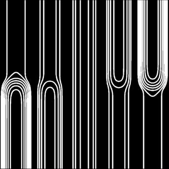
80 > Simulation results Contour plots of fine scale solution (solid lines) and reconstructed reduced solution (dotted lines) for µ 1 = 0.85, µ 2 = 0.5, µ 3 = 0.1 ( T h = 32768). Difference between fine scale and reduced solution. Coarse triangulation (black) with number of reduced basis functions Φ F ( T h = 2048/32768, respectively).,

81 , > CPU times for the new method Averaged runtimes over 125 simulations: high and low dimensional algorithms (t highdim and t lowdim ); the reconstruction (t recons) and mean relative errors ( p λ h p λ N L 2/ p λ h L 2) for different grid sizes.

82 Thank you for your attention! Software: DUNE, DUNE-FEM, RBmatlab, DUNE-RB

83 Thank you for your attention! Software: DUNE, DUNE-FEM, RBmatlab, DUNE-RB PDESoft2012: Workshop on PDE Software Frameworks 10th Anniversary of DUNE June 18-20, 2012, Muenster, Germany. MoRePaS II: Second International Workshop on Model Reduction for Parametrized Systems Oct 2-5, 2012, Schloss Reisensburg, Guenzburg, Germany.