ABSTRACT TRANSIENT TEMPERATURE MEASUREMENTS OF COMBUSTOR WALLS ENCLOSING A 2-D MODEL COAXIAL INJECTOR. Hak Seung Lee, Master of Science, 2013

Transcription

1 ABSTRACT Title of Document: TRANSIENT TEMPERATURE MEASUREMENTS OF COMBUSTOR WALLS ENCLOSING A 2-D MODEL COAXIAL INJECTOR Hak Seung Lee, Master of Science, 2013 Directed By: Associate Professor, Kenneth H. Yu, Department of Aerospace Engineering Direct measurements of combustor inner wall temperatures are difficult due to harsh flow conditions. A novel approach was used to obtain the combustor wall temperature as a function of time and location in a H2-O2 model injector, enclosing acoustically forced flames. The emphasis was to obtain thermal boundary conditions for various injector operation. The new approach combined a series of experimental measurements on the outer wall with a transient heat transfer analysis applicable for low Biot number and low Fourier number conditions. Infrared thermometry technique was applied to obtain outer wall temperature distribution at three different wall thicknesses, and these measurements were combined with the transient analysis to calibrate the amount of heat transfer and the corresponding inner wall temperature. The results showed that the combustor inner wall temperature distribution evolved much differently for acoustically forced flames, suggesting a different thermal boundary condition should be used in those cases.

2 TRANSIENT TEMPERATURE MEASUREMENTS OF COMBUSTOR WALLS ENCLOSING A 2-D MODEL COAXIAL INJECTOR By Hak Seung Lee Thesis submitted to the Faculty of the Graduate School of the University of Maryland, College Park, in partial fulfillmemt of the requirements for the degree of Master of Science 2013 Advisory Committee Dr. Kenneth Yu, Chair Dr. Chris Cadou Dr. Raymond Sedwick

3 Copyright by Hak Seung Lee 2013

4 Dedication To my wife and family, for all their love and support. ii

5 Acknowledgements I would like to thank my advisor, Dr. Yu, for his guidance and assistance on this project and throughout my graduate career. I would also like to Dr. Cadou and Dr. Sedwick for their time and critical evaluation as my committee members. I am especially grateful to Dr. Amardip Ghosh and Qina Diao for helping me in conducting many of the experiments reported in this work. I would also like to thank my colleagues, Sammy Park, Camilo Aguilera, and others, for helping me out with this work and having a great time in the office and campus area. I would also like to acknowledge the funding that made this research possible. This work was sponsored by a grant from NASA CUIP. I would like to thank Tom Nesman of NASA- Marshall for his help with various aspects of this project. iii

6 Table of Contents Dedication...ii Acknowledgements...iii Table of Contents...iv List of Figures and Tables...vi Table of Nomenclature...xiii Chapter 1:Introduction Background and Motivation Objectives and Scope...5 Chapter 2: Literature Review Combustion Instability Instabilities in Liquid Rocket Engines Shear Coaxial Injectors Flame-Acoustic Interactions Loci-CHEM Applications Inner Wall Temperature Measurement Cold Flow Experiments Reacting Flow Experiments Loci-CHEM CFD Simulations...20 Chapter 3: Experimental Setup Overview of Setup Description of Apparatus Combustor Geometry Inlet and Feed Systems Acoustic Loudspeaker Flame Images and Wall Temperature Measurement Ignition and Extinction a Ignition b Extinction...38 Chapter 4. Analytical Consideration Basic Physical Mechanisms Heat Transfer Equation and Wall Temperature Solution Non-dimensional Parameters Fourier Number Biot Number...53 Chapter 5. Wall Temperature Measurements and Deduction Introduction Baseline Cases (without acoustic forcing) Temperature Measurements of Each Location for Baseline Cases Acoustic Forcing Cases Temperature Measurements of Each Location for Acoustic Forcing Cases Combined Temperature Distributions Temperature Distributions Based on Fourier Number...76 iv

7 5.6 Inner Wall Temperatures Comparison between Experimental and Analytical Results Procedure to Extrapolating Wall Temperature Function Instantaneous Flame Images Uncertainty of the Measurements Measurement Uncertainty Revision of Temperature Range Deformation of Combustor Wall Temperature Aberration from Camera Lens Chapter 6. Concluding Remarks and Future Work Summary Key Contributions Concluding Remarks Future Work Bibliography v

8 List of Figures and Tables Figure 2.1: Attempt of Silicon Wafer for direct measurements Figure 2.2: Baseline Schlieren images for H2/Air/Heat 10/6/18 m/s Figure 2.3: Phase-locked Schlieren images for He/Air/He with acoustic forcing at 400Hz and 40Hz Figure 2.4: Phase-locked Schlieren images for He/Air/He with acoustic forcing at 771Hz and 40Hz Figure 2.5: Schlieren images for He/Air/He with acoustic forcing at 771Hz, (a) 20vpp (b) 30vpp (c) 40vpp (d) 50vpp Figure 2.6: OH* Chemiluminescence showing baseline state of turbulent H2/O2/H2 flames at 18/6/18 m/s Figure 2.7: Phase-Locked OH* Chemiluminescence showing H2/O2/H2 flames forced at 300Hz Figure 2.8: Phase-Locked OH* Chemiluminescence showing H2/O2/H2 flames forced at 1150Hz Figure 2.9: Comparison of experiments and CFD of flame-acoustic interaction: (a) Phase-locked Schlieren images with forcing at 405Hz, (b) Zoomed view of near-injector field showing density gradient magnitude with forcing at 405Hz Figure 2.10: Comparison of experiments and CFD of flame-acoustic interaction: (a) Phaselocked Schlieren images with forcing at 885Hz, (b) Zoomed view of near-injector field showing density gradient magnitude with forcing at 885Hz Figure 2.11: Comparison of experiments and simulation of flame-acoustic interaction: (a) Standing wave excitation at 300Hz, (b) Traveling wave excitation at 1150Hz vi

9 Figure 3.1: Combustor setup showing model injector experiments for flame-acoustic interaction Figure 3.2: Schematic showing region of real injector field being modeled by experimental setup Figure 3.3: Overview of combustor geometry Figure 3.4: Pictures of the experimental setup, (a) side view, (b) front view Figure 3.5: Technical drawing of combustor inlets Figure 3.6: Picture showing cutaway of combustor inlets Figure 3.7: Picture of gas inlet feed lines Figure 3.8: Combustor setup showing model injector experiments for flame-acoustic interaction Figure 3.9: Four different locations for the temperature measurement with IR thermometry Figure 3.10: Dimension of the combustor measurement wall holder Figure 3.11: IR thermometry, FLIR ThermalCAM SC3000 Table 3.1: Temperature range of IR thermometry Figure 4.1: Baroclinic interactions between density gradient and pressure fradient at a density stratified interface: (a) Unstable interaction (b) Stable interaction Figure 4.2: Controlled compression waves toward the combustor by acoustic driver Figure 4.3: Acoustic resonance characteristics of the combustor Figure 4.4: Illustration of combustor wall temperature profile and its evolution in time Figure 4.5: Computed wall temperature changes as (a) a function of time, and (b) a function of combustor wall thickness Figure 4.6: High temperature zone of the combustor wall, directions of heat transfer, and the corresponding length scale Figure 4.7: Average temperature versus Fourier number for three different combustor wall thickness vii

10 Figure 5.1: Wall temperature measurements for unforced cases with three different thicknesses at the 1st floor: (a) 1/32 inch, (b) 1/16 inch, (c) 1/8 inch Figure 5.2: Wall temperature measurements for unforced cases with three different thicknesses at the 2nd floor: (a) 1/32 inch, (b) 1/16 inch, (c) 1/8 inch Figure 5.3: Wall temperature measurements for unforced cases with three different thicknesses at the 3rd floor: (a) 1/32 inch, (b) 1/16 inch, (c) 1/8 inch Figure 5.4: Wall temperature measurements for unforced cases with three different thicknesses at the 4th floor: (a) 1/32 inch, (b) 1/16 inch, (c) 1/8 inch Figure 5.5: Wall temperature measurements for acoustic forcing cases with three different thicknesses at the 1st floor: (a) 1/32 inch, (b) 1/16 inch, (c) 1/8 inch Figure 5.6: Wall temperature measurements for acoustic forcing cases with three different thicknesses at the 2nd floor: (a) 1/32 inch, (b) 1/16 inch, (c) 1/8 inch Figure 5.7: Wall temperature measurements for acoustic forcing cases with three different thicknesses at the 3rd floor: (a) 1/32 inch, (b) 1/16 inch, (c) 1/8 inch Figure 5.8: Wall temperature measurements for acoustic forcing cases with three different thicknesses at the 4th floor: (a) 1/32 inch, (b) 1/16 inch, (c) 1/8 inch Figure 5.9: Process to make a whole combined image from the results of four different locations Figure 5.10: Time evolution of combustor outer-wall temperature distribution under the baseline unforced conditions. The corresponding wall thicknesses for temperature measurements were: (a) 1/32 inch, (b) 1/16 inch, (c) 1/8 inch Figure 5.11: Time evolution of combustor outer-wall temperature distribution under acoustically forced conditions. The forcing frequency was 1150Hz,and the corresponding wall thicknesses for temperature measurements were: (a) 1/32 inch, (b) 1/16 inch, (c) 1/8 inch viii

11 Figure 5.12: Measurement of horizontal temperature profiles for baseline case at the 4 inches from the bottom line: (a) corresponding t = 15 sec, (b) temperature t = 5 sec, (c) temperature t = 10 sec, (d) temperature t = 15 sec Figure 5.13: Horizontal temperature profiles at 4 inches from the bottom line: (a) temperature profiles for t = 5 sec, (b) temperature profiles for acoustic t = 5 sec, (c) temperature profiles for t = 10 sec, (d) temperature profiles for acoustic t = 10 sec, (e) temperature profiles for t = 15 sec, (f) temperature profiles for acoustic t = 15 sec Figure 5.14: Horizontal temperature profiles at 7 inches from the bottom line: (a) temperature profiles for t = 5 sec, (b) temperature profiles for acoustic t = 5 sec, (c) temperature profiles for t = 10 sec, (d) temperature profiles for acoustic t = 10 sec, (e) temperature profiles for t = 15 sec, (f) temperature profiles for acoustic t = 15 sec Figure 5.15: Horizontal temperature profiles at 10 inches from the bottom line: (a) temperature profiles for t = 5 sec, (b) temperature profiles for acoustic t = 5 sec, (c) temperature profiles for t = 10 sec, (d) temperature profiles for acoustic t = 10 sec, (e) temperature profiles for t = 15 sec, (f) temperature profiles for acoustic t = 15 sec Figure 5.16: Average temperature versus Fourier number for three different combustor wall thickness assumed Lc y Figure 5.17: Average temperature versus Fourier number for three different combustor wall thickness assumed Lc ( ) z x y 1/ 3 ix

12 Figure 5.18: Average temperature versus Fourier number for three different combustor wall thickness assumed Lc x y Figure 5.19: Combustor wall temperature distributions associated with unforced flames as a function of Biot number and Fourier number Figure 5.20: Combustor wall temperature distributions associated with flame-acoustic interaction as a function of Biot number and Fourier number Figure 5.21: Measurement of horizontal temperature distributions at three different heights: 4, 7 and 10 inches from the bottom line. (a) corresponding images for Fo = 20, (b) corresponding images for acoustic Fo = 20 Figure 5.22: Horizontal temperature profiles at 4 inches from the bottom line: (a) temperature profiles for Fo = 10, (b) temperature profiles for acoustic Fo = 10, (c) temperature profiles for Fo = 15, (d) temperature profiles for acoustic Fo = 15, (e) temperature profiles for Fo = 20, (f) temperature profiles for acoustic Fo = 20, (g) temperature profiles for Fo = 25, (h) temperature profiles for acoustic Fo = 25 Figure 5.23: Horizontal temperature profiles at 7 inches from the bottom line: (a) temperature profiles for Fo = 10, (b) temperature profiles for acoustic Fo = 10, (c) temperature profiles for Fo = 15, (d) temperature profiles for acoustic Fo = 15, (e) temperature profiles for Fo = 20, (f) temperature profiles for acoustic Fo = 20, (g) temperature profiles for Fo = 25, (h) temperature profiles for acoustic Fo = 25 Figure 5.24: Horizontal temperature profiles at 10 inches from the bottom line: (a) temperature profiles for Fo = 10, (b) temperature profiles for acoustic Fo = 10, (c) temperature profiles for Fo = 15, (d) temperature profiles for acoustic Fo = 15, (e) temperature profiles for Fo = 20, (f) temperature profiles for acoustic Fo = 20, (g) temperature profiles for Fo = 25, (h) temperature profiles for acoustic Fo = 25 x

13 Figure 5.25: Combustor outer wall temperature as a function of combustor wall thickness and forcing condition at certain instants after ignition Figure 5.26: Comparison of analytical and experimental results for combustor outer wall temperature as a function of time (seconds) with baseline case. (a) corresponding image, (b) results of the whole combustor area, (c) results of the local area in the rectangle Figure 5.27: Comparison of analytical and experimental results for combustor outer wall temperature as a function of time (seconds) with acoustic forcing case. (a) corresponding image, (b) results of the whole combustor area, (c) results of the local area in the rectangle Figure 5.28: Deduced inner wall temperature along with measured outer wall temperature distributions at select wall thicknesses and under various flow conditions for baseline cases Figure 5.29: Deduced inner wall temperature along with measured outer wall temperature distributions at select wall thicknesses and under various flow conditions for acoustic forcing cases Figure 5.30: Measurement of horizontal temperature distributions at three different heights: 4, 7 and 10 inches from the bottom line. (a) corresponding images for t = 10sec, (b) corresponding images for acoustic t = 10sec Figure 5.31: Horizontal temperature profiles at 4 inches from the bottom line: (a) temperature profiles for t = 5 sec, (b) temperature profiles for acoustic t = 5 sec, (c) temperature profiles for t = 10 sec, (d) temperature profiles for acoustic t = 10 sec, (e) temperature profiles for t = 15 sec, (f) temperature profiles for acoustic t = 15 sec xi

14 Figure 5.32: Horizontal temperature profiles at 4 inches from the bottom line: (a) temperature profiles for t = 5 sec, (b) temperature profiles for acoustic t = 5 sec, (c) temperature profiles for t = 10 sec, (d) temperature profiles for acoustic t = 10 sec, (e) temperature profiles for t = 15 sec, (f) temperature profiles for acoustic t = 15 sec Figure 5.33: Horizontal temperature profiles at 4 inches from the bottom line: (a) temperature profiles for t = 5 sec, (b) temperature profiles for acoustic t = 5 sec, (c) temperature profiles for t = 10 sec, (d) temperature profiles for acoustic t = 10 sec, (e) temperature profiles for t = 15 sec, (f) temperature profiles for acoustic t = 15 sec Figure 5.34: Comparison of flame-acoustic interaction under various thickness walls and combustor conditions Figure 5.35: Example of the temperature uncertainty and revision at the 4 inches from the bottom line and econds after the ignition: (a) measured temperature distribution before revision, (b) temperature distribution after temperature revision Figure 5.36: Temperature revision by a quadratic parabolic equation: dashed red line - measured temperature by IR thermometry, solid blue line - revised new temperature Figure 5.37: Example of the plate burning and warping Figure 5.38: Elimination of the dark spot on the wall temperature profile. (a) with original surface, (b) after scratching the surface xii

15 Table of Nomenclature Hz vpp ω ρ u v t d λ G T q' p' δ h k x y z cp A = Frequency of the acoustic driver = Volts Peak-to-Peak (Acoustic Forcing Amplitude) = Vorticity = Density of the metal window = Velocity in the x axis = Velocity in the y axis = time from the instant of ignition = diameter = wavelength = Rayleigh index = Temperature = Fluctuating component of heat release = Fluctuating component of pressure = Wall thickness = Heat transfer coefficient = Thermal conductivity of the metal window = Distance in transverse direction = Distance in streamwise direction = Distance in vertical direction = Heat capacity of the metal window = Area xiii

16 θ α Lc Fo Bi m γ = Normalized temperature = Thermal diffusivity = Characteristic length = Fourier numbera = Biot number = Mass flow = Ratio of specific heats A* = Choked orifice area R GH2 GO2 RT RM = Specific gas constant = Gaseous Hydrogen = Gaseous Oxygen = Rayleigh-Taylor Instability = Richtmyer-Meshkov Instability xiv

17 Chapter 1. Introduction 1.1 Background and Motivation Combustion instabilities in the liquid rocket engines have remained a continued interest of study since their discovery in the late 1930s (Culick and Yang 1995). Combustion instability takes place when high amplitude pressure oscillations are coupled with heat release fluctuations (Rayleigh 1945, Culick 1987). In particular, high frequency instability in liquid rocket engines may affect the structure critically, applying large pressure loads and increased heat transfer rates. Unfortunately, it remains to be unpredictable. Without an acceptable solution, the appearance of instabilities can delay the development of new engine design (Hulka and Hutt 1994). Instabilities in rocket engines can be classified into two categories: low frequency and high frequency instabilities. Low frequency instabilities are generated by a coupling between the combustion and the propellant feed lines. High frequency instabilities have two different modes: tangential and radial modes of the combustion chamber. In the liquid rocket engine combustion chamber, tangential and radial transverse waves interact with heat released at high frequency and high pressure oscillation (Culick and Yang 1995, Rubinsky 1995). Critical damage to the structural and control components can be attributed to these instabilities, and high heat release rates can generate devastating burnouts (Reardon 1961, Male 1954, Reardon 1967, Ebrahimi 2000). Harrje and Reardon (1972) observed, then divided combustion instabilities into three categories based on their frequencies: chugging, screaming, and buzzing. Low frequency instability (chugging) is typically observed when frequencies are less than a few hundred Hz. 1

18 High frequency combustion instability (screaming) is the result of the closeness measured in pressure oscillation frequencies to the computed acoustic resonance modes of the thrust chamber. It is not influenced by the propellant feed system of the rocket engine. An intermediate frequency (buzzing) consists of lumping together the resulting instabilities that do not fall into either chugging or screaming. The interaction between the acoustic wave and the flow creates atomization, mixing, and burning in the near-injector region. This acoustic fluctuation may affect the mixing, atomization, vaporization, and other functions performed by the combustion in the propulsion system. A turbulent diffusion flame is formed at the interface as the LOX atomizes or mixes with gaseous hydrogen. These shear-coaxial injectors have been used in a large number of rocket engines, including the space shuttle main engines. Most of the physical mechanisms of instabilities are present in the near-injector region which consists of higher velocity and density gradients (Kim and Williams 1998, Oefelein and Yang 1997). After several decades, it still remains unclear which mechanism is the leading factor causing instability in the injector (Glogowski et al. 1994). Strong amplitude pressure waves in this region can cause oscillatory heat release, and coupled with the acoustic waves. It has the possibility of increasing the amplitude of the pressure waves. Acoustic waves which interact with the flame in the combustor have been categorized into two separate types of pressure waves: standing and traveling waves. Both waves have been researched through experimental and theoretical studies for several decades. The amplitude of acoustic disturbances can generate large amplitude of heat release at certain circumstances (Rayleigh and Lord 1945, Sreenivasan and Raghu 2000). Acoustic pressure amplitudes of the tangential modes are notably higher in the near-injector region than near the nozzle because of the higher density levels near the injector (Kim and Williams 1998). Density differences lead to 2

19 increase sensitivity of acoustic instabilities near the injector field. Most of the physical mechanisms surrounding combustion instability occur at the near injector region. Thus, the scope of this research was purposely restricted to flame acoustic interactions occurring in the near field of the shear coaxial injector. The LOX jet is atomized and vaporized in the combustor chamber, and a diffusion flame is formed in the near-injector area between gaseous oxygen and hydrogen. This flame-acoustic coupling causes spatial heat release fluctuation and pressure oscillations generated by this acoustic force ultimately drive the combustor to unstable levels. The flame instability of the shear layer between the fuel and oxidizer in the injector can be amplified by certain modes of acoustic oscillation without notice. The velocity difference between fuel and oxidizer generates Kelvin-Helmholtz instability on the interface (Rehab et al. 1997), and the chemical reaction between fuel and oxidizer on the interface can drive thermodiffusive instabilities (Matalon 2007, Kim et al. 1996). The density stratified interface between fuel and oxidizer becomes susceptible to instibilities by the interactions with pressure waves generated through acoustic excitation. A Richtmyer-Meshkov (RM) instability and a Rayleigh-Taylor (RT) instability are generated from the density stratified interface (Taylor 1950, Richtmyer 1960, Meshkov 1969). Small amplitude acoustic disturbances can lead to significant increases of amplitude levels in the flame surface area. Small changes of the circumstance in combustors such as velocity ratio, momentum ratio, temperature, and pressure may create significant effects on the overall stability of the engine (Hulka and Hutt 1995). Previously, flame acoustic interactions in the near injector field of a shear coaxial injector were experimentally researched to determine key factors for acoustically driven instabilities in liquid rocket engine injectors. The amount of interaction between flame and acoustic force is strongly dependent on the density ratio between two different fluids. This 3

20 examination is in accordance with the baroclinic vorticity mechanism and a Rayleigh-Taylor instability mechanism. Computational fluid dynamic (CFD) methods have been used as a practical tool for the design and development of propulsion systems for several decades. However, capturing appropriate combustion instability for the propulsion systems remains a challenge. The benefits associated with predicting the instabilities using the CFD method are to save time and money during the design process. The CFD method can also benefit the analysis of existing systems which have instability issues. The use of CFD has the potential to improve the design of liquid rocket propulsion systems by simulating the sensitivity of performance and thermal environments of the injector geometry (Tucker 2007, Tsohas 2007). Unfortunately, existing accuracy problems associated with CFD cause decreased utility. In order to predict combustion instabilities, it may be essential to simulate such flame-acoustic interaction accurately. Conversely, a detailed dataset on flameacoustic interaction can be quite useful for assessing and validating various simulation methods. A comprehensive dataset, including the proper boundary conditions, can be used to validate CFD results and assess the usefulness in instability studies. Our subsequent simulation efforts using a LOCI framework failed to capture certain features of the flame-acoustic interaction. (Gers et al. 2010). In particular, asymmetric flame-acoustic interaction observed under traveling-wave mode excitation was not observed in the simulation. One potential problem witnessed in the simulation refers to thermal boundary conditions. It would appear not enough information exists, causing a new issue. Here, an adiabatic assumption was used for the combustor wall boundary as a substitute for insufficient data, even though the experiments were run without any insulator. It is desirable to investigate the cause and obtain more detailed data on boundary conditions. 4

21 1.2 Objectives and Scope Previously, Ghosh et al. (2006, 2007) studied the onset of flame-acoustic interaction which affected the instability of a shear coaxial injector. He described flame oscillations from the interaction between turbulent diffusion flame and compression waves being amplified at certain frequencies. Gers et al. (2010) performed numerical simulations to predict dynamic interactions between hydrogen-oxygen turbulent diffusion flames and pressure waves. The simulations were conducted in a LOCI-Chem framework, with the following boundary conditions: fixed mass flux inflow, fixed pressure outflow, viscous adiabatic walls, and oscillating acoustic driver. Here, the thermal boundary condition of an adiabatic wall was used, but it remains to be improved since the combustor wall is not adiabatic in real conditions. The objective of the present work is to obtain detailed measurements on the combustor inner wall temperature as a function of acoustic forcing. Such direct measurements, both spatially and temporally resolved, can not only be used to understand the nature of flameacoustic interaction but they can also provide experimental data for CFD validation. The scope is limited to the current combustor geometry where we already have detailed flow measurements available. The measured temperature will be used to set up thermal boundary conditions for predicting reacting flow behavior with and without acoustic excitation. The focus of this work was to obtain thermal boundary conditions of the combustor inner wall. The technical objectives of this work are as follows: 1. To study the flame acoustic interaction in an H2-O2 model shear coaxial injector 2. To assess the capabilities of various reacting flow solvers in simulating flame-acoustic interaction 5

22 3. To build an experimental database for validating CFD simulation 4. To measure combustor wall temperature distribution during the injector experiments 5. To establish proper thermal boundary conditions for flame-acoustic interaction simulation 6

23 Chapter 2. Literature Review 2.1 Combustion Instability Combustion instabilities have been a significant issue in the last several decades, and a significant amount of research has been done with emphasis on combustion instability related to liquid rocket engines. The Rayleigh criterion has been regarded highly in the combustion instability field due to its significant and purposeful work. This criterion explains that the total acoustic energy of the system will be increased when the pressure fluctuation p' and heat release fluctuation q' are in phase with each other. Putnam and Dennis (1954) derived a mathematical verification between pressure and heat release oscillations. They developed Rayleigh criteria in a more detailed form by extending the wave equation for acoustic motions and creating a more precise expression with p' and q' to the energy change in the system. Later, Chu et al. derived a generalized form of Rayleigh's criterion by using the concept of energy in small disturbance circumstances (Chu 1965). Barerre and Williams divided combustion instabilities into three types: intrinsic instabilities, system instabilities, and chamber instabilities (Barerre 1969). Later, chamber instabilities were reclassified again into acoustic instabilities, shock instabilities, and fluid-dynamic instabilities. 2.2 Instabilities in Liquid Rocket Engines Combustion instabilities on liquid rocket engines were first studied in the early 1940s (Culick and Yang 1995). Summerfield et al. observed and discussed that time delay is one of the 7

24 most important factors of the liquid rocket combustion instability (Summerfield 1951). A finite time delay is generated when a propellant enters the combustor which forces heat to be released. Crocco analyzed high frequency instability based on varying combustion time lag, which introduced two different time lags: a constant time lag, and a varying time lag (Crocco 1951, 1952). Crocco and Cheng investigated longitudinal mode combustion instability (Crocco and Cheng 1956), and time lag theory of transverse mode instabilities were examined by Scala (1957). These are all theoretical approaches without any experimental verifications. So, thereafter, Crocco et al. showed experimental results for the time lag theory to justify the theoretical approaches (Crocco 1960). The 'screaming' instabilities with high frequency in liquid rocket engines were investigated through the use of experiments by Male et al (Male 1954). In this case, the heat transfer was substantially increased, and the heat transfer was noticeably larger for transverse modes than longitudinal modes. The experiments also showed that the transverse mode of the instabilities were dominant in the near-injector region. Baker and Steffen conducted experiments to study screaming of the GH2/LOX propellant mixture with high frequency response case in the liquid rocket injector. They showed that a mixture of liquid and gaseous propellant makes lower screaming than all-liquid propellant cases (1958). Osborn and Bonnel (1960) investigated the effects of chamber geometry, pressure and chemical reactions on combustion instability in a gas rocket. The instability was affected on the different conditions with both longitudinal and transverse modes. Rupe and Jaivin (1964) experimentally showed the resonant effects and mass flux distribution on combustion heat transfer rates in liquid rocket engines. Wanhainen et al. investigated the factors which affect the combustor stability in the liquid rocket engine (Wanhainen 1966). Propellant injection area, velocity, tube geometry and recess 8

25 were considered as attributing factors of instability issues. Reardon et al. (1967) showed radial and tangential velocity effects to influence the combustion process rates. Tangential velocity fluctuation largely affects the tangential modes of oscillations but has no effect on the standing modes. Fluctuations of radial velocity have a relatively smaller effect on the oscillations. Wanhainen et al. examined suppression of high frequency combustion instability with acoustic damping devices in liquid rocket engines (Wanhainen 1967). They showed acoustic damping at the wall of the combustion chamber affects its stability limit and frequencies. Barsotti et al. (1968) showed the velocity ratio of fuel and oxidizer affects its stability in LOX/LH2 liquid rocket engines. Higher velocity ratio and fuel injection temperature could improve the combustor's stability. Zinn and Savell (1969) showed the influence of Mach number, combustor length and nozzle convergence on the linear stability of the three-dimensional liquid rocket combustor. Priem et al. (1969) studied the influence of those factors theoretically. They used irrotational wave equations coupled with the boundary conditions at the injector wall, nozzle entrance and the acoustic liners. Zinn et al. (1971) looked at non-linear combustion instability in liquid rocket engines. A non-linear wave equation was used to express flame oscillation. Culick et al. (1975) provided a formal framework by which practical problems can be treated with a minimum of effort. They analyzed the nonlinear growth and limiting amplitude of acoustic waves in a combustion chamber. Combustion instabilities in liquid rocket engines with linear and non-linear waves have been reviewed and discussed in the 1990s (Mitchell 1994, Culick 1995). They described the association between the injection system and combustion chamber for exciting and sustaining combustion instabilities with linear or non-linear behavior. Fischbach et al. (2007) studied 9

26 acoustic effects with traveling transverse wave oscillation and showed the effects could accelerate the amplitude of the wave fronts. 2.3 Shear Coaxial Injectors Since shear coaxial injectors were used for experiments and CFD work in this research, it is necessary to look at a brief overview of this type of injector. There are two kinds of injectors in liquid rocket engines: shear coaxial injector and swirl coaxial injector. The shear coaxial injector was developed in the late 1940s and became the favored injector for liquid rocket engines in the United States during this time. In the late 1950s experimental research related to various parameters about engine stability were conducted (Hulka and Hutt 1994). Combustor geometry, temperature, pressure, injection velocity and recess existence were all main factors to influence the stability of the rocket engine. Oefelein et al. (1997) performed experimental works about important parameters for shear coaxial injectors. They showed that velocity ratio, density ratio and momentum ratio are key factors of the propellant streams. 2.4 Flame-Acoustic Interactions Combustion instability occurs due to the coupling of pressure fluctuation and heat release. Flame interaction by acoustic instabilities can affect overall operation and provide significant insight to the development of liquid rocket engines. McIntosh et al. (1991) showed the interaction of pressure disturbances characterized by different length scales with conventional flames. Richecoeur et al. (2006) investigated high-frequency combustion oscillations 10

27 experimentally with cryogenic propellants under elevated pressure conditions. This study focused on high-frequency dynamics resulting from a strong coupling between one of the transverse modes and combustion. Lang and Poinsot (1987) generated external acoustic excitation by a loudspeaker to suppress the oscillation of a flame. Suzuki and Atarashi (2007) explored the effect of acoustic excitation on jet diffusion flames. They investigated the behavior and structure of a methane jet inside a flame corresponding to acoustic forcing. Ghosh et al. (2008) investigated key physical mechanisms influencing flame-acoustic coupling during the combustion instabilities in liquid rocket engines. They set up a twodimensional shear coaxial liquid rocket injector model and excited acoustic force by a compression driver in a transverse direction with a wide range of frequencies and amplitudes. They showed that flame-acoustic interaction is most susceptible to the density ratio changes between the fuel and oxidizer. 2.5 Loci-CHEM Applications A lot of computational simulation works have been conducted to predict flame-acoustic interactions. Loci-CHEM, developed at Mississippi State University, is one of the powerful numerical solvers for these propulsion systems. Lin et al. (2005) used Loci-CHEM codes to simulate a shear coaxial single element GO2/GH2 injector experiment. The Loci-CHEM solution matches both the heat flux rise rate in the near injector region and the peak flux level. Tsohas and Canino (2007) used Loci-CHEM code to perform single-element, 2-D unsteady CFD computations on the Hydrogen-Oxygen multi-element experiment injector. Parametric studies on O/F ratio, LOX post thickness and hydrogen inlet temperature were executed to evaluate their effects. Roy and Tendean (2007) operated Loci-CHEM code to solve the steady-state, 11

28 compressible RANS equations in 2-D cases. Hughson and Luke (2008) applied Loci-CHEM for a two-species model composed of air and rocket exhaust gas with a RANS flow solver. They used a hybrid RANS/LES solver for two explicit turbulence models with 10 to 100 mph free stream wind speed. Gers et al. (2010) executed Loci-CHEM CFD solver to simulate flame interaction between hydrogen and oxygen in the turbulent diffusion flames for liquid rocket engine shear coaxial injectors. 2.6 Inner Wall Temperature Measurement Direct measurements of inner wall temperatures in the combustion chamber are difficult to determine. The first problem is related to the point where an accurate measurement can take place. Unfortunately, the chamber is closed and too hot for the measuring apparatus to even reach. The second pitfall for accurate inner wall temperature measurement is lack of information for the values in the chamber. Thermocouples could be used for this experiment because they have been widely used for direct temperature measurements and can measure very high temperature with good accuracy. However, the area of measurement is very limited with a thermocouple. Only a single point can be measured with a thermocouple at one time. The temperature distributions of the whole combustor area were necessary in this experiment, and IR thermography is useful to obtain temperature distributions of certain areas. For this reason, IR thermometry was selected for this experimental work. There have been several novel efforts for measuring the inside wall temperatures in combustion systems. Shedd et al. (2005) used thermoreflectance for inner wall temperature measurements on a copper tube surface. Jiang et al. (2012) offered a method for calculating an 12

29 inner wall temperature from measurement results of an outer wall temperature of a tube. They estimated inner wall temperatures on the basis of the measured outer wall temperatures by evaluating a plurality of points under a two-dimensional unsteady flow in the tube. For the inner wall temperature measurements, silicon wafer was first attempted for direct measurements using IR thermography. A very thin (0.025 inch thickness) round-shaped silicon wafer was used for this experiment. However, the silicon wafer was cracked a few seconds after ignition as shown in Fig 2.1. Then, the silicon wafer was replaced by stainless steel for indirect measurements. Here, a new approach to obtain inner wall temperatures of the combustor was proposed. In this experiment, the outer wall temperature of three different thicknesses of metal were measured and extrapolated to calibrate inner wall temperatures with transient heat transfer analysis. IR-thermometry was used to obtain the whole temperature profile of the combustor wall. Fig. 2.1 Attempt of Silicon Wafer for direct measurements 13

30 2.7 Cold flow Experiments Cold flow experiments were executed with helium and air to observe acoustic forcing effect to the flow field in the combustion chamber without heat release. In the experiments velocities were all fixed at 6m/s for air and 18m/s for helium, and acoustic forcing was provided at a range of frequencies. The schlieren images for the baseline case without acoustic forcing are shown in Fig. 2.2, and Fig 2.3 shows the cases of acoustic forcing at 400Hz and 40vpp. The flow acoustic interactions were observed symmetric at this frequency for both sides although acoustic forcing was generated at one side. Fig. 2.2 Baseline Schlieren images for He/Air/He at 18/6/18 m/s (Ghosh, 2008) 14

31 Fig. 2.3 Phase-locked Schlieren Images for He/Air/He with acoustic forcing at 400Hz and 40vpp (Ghosh, 2008) Fig. 2.4 shows the schlieren images of cold flow with acoustic forcing at 771Hz and 40vpp. At this frequency, the asymmetric flow interaction was observed with acoustic forcing, and the flow was inclined to the side of the acoustic forcing. Fig. 2.5 shows the images of flow interaction with several different amplitudes from 20vpp to 50vpp at the constant frequency of 771Hz. 15

32 Fig. 2.4 Phase-Locked Schlieren images for He/Air/He with acoustic forcing at 771Hz and 40vpp (Ghosh, 2008) 16

33 Fig. 2.5 Schlieren images for He/Air/He with acoustic forcing at 771Hz, (a) 20vpp (b) 30vpp (c) 40vpp (d) 50vpp (Ghosh, 2008) 2.8 Reacting Flow Experiments The reacting flow experiments were executed with hydrogen and oxygen to observe flame interaction with acoustic forcing condition in the combustion chamber. The velocity ratios were kept at the same condition of 6m/s for oxygen and 18m/s for hydrogen, and an igniter was used to ignite the flame to the chamber. OH* Chemi-luminescence and a high speed ICCD camera were used to capture the images of the flame. Fig. 2.6 shows the OH* Chemi- 17

34 luminescence image for baseline case, without acoustic forcing. Fig. 2.7 shows the instantaneous flame images with 300Hz of acoustic forcing, and flames were shown almost symmetric in this frequency. On the other hand, strong asymmetric flame interactions were observed at the frequency of 1150Hz as shown in Fig 2.8. The flame on the side of the speaker displayed much oscillation. However, the flame on the other side was relatively stable. Because the density gradient is pointing in opposite directions on each side of the center jet, the resulting torque amplifies the flame disturbances near the speaker. Fig. 2.6 OH* Chemiluminesence showing baseline state of turbulent H2/O2/H2 flames at 18/6/18 m/s 18

35 Fig. 2.7 Phase-Locked OH* Chemiluminesence showing H2/O2/H2 flames forced at 300Hz Fig. 2.8 Phase-Locked OH* Chemiluminesence showing H2/O2/H2 flames forced at 1150Hz 19

36 In addition, as the density ratio decreases, the flame oscillation becomes more stable under the same frequency of acoustic forcing. The Ph.D dissertation of Ghosh (2008) introduced more detailed results about these experiments. 2.9 Loci-CHEM CFD Simulations A numerical simulation was performed by Gers et al. to predict flame interaction between oxygen-hydrogen with Loci-CHEM solver. The boundary conditions for the numerical simulations were set up at the same conditions with the Ghosh's experiments as much as possible. The flow velocities of inlets were fixed at the same value of the experiments, 6m/s for oxygen and 18m/s for hydrogen. Based on the frequency of the acoustic driver, the flame structures were formed either symmetric or asymmetric. Both cold and reacting flows were simulated with several different frequencies of acoustic forcing. Fig. 2.9 shows the comparison between experimental image and Loci-CHEM simulation results in the cold flow for the baseline case with 405Hz of acoustic forcing. At this frequency, the products from the CFD method appeared qualitatively close to the experimental results. Fig shows the comparison between experimental and computational results for the 885Hz acoustic forcing case. At this frequency, an asymmetric flame was observed in the CFD results, and this corresponds with the experimental results as well. 20

37 (a) (b) Fig. 2.9 Comparison of experiments and CFD of flame-acoustic interaction: (a)phase-locked Schlieren images with forcing at 405Hz (b) Zoomed view of near-injector field showing density gradient magnitude with forcing at 405Hz (Gers, 2010) (a) (b) Fig 2.10 Comparison of experiments and CFD of flame-acoustic interaction: (a) Phase-locked Schlieren images flow with forcing at 885Hz (b) Zoomed view of near-injector field showing density gradient magnitude with forcing at 885Hz (Gers, 2010) 21

38 The Loci-CHEM simulations for the reacting flow were also performed at two different frequencies, 300Hz and 1150Hz. Symmetric flame-acoustic interactions were created under standing wave excitation, and traveling wave excitations produced asymmetric flame interactions. Both symmetric (300Hz) and asymmetric (1150Hz) flame interactions were represented by Loci- CHEM CFD solver and compared with the experimental results as shown in Fig Some ripple effects were observed in the flame for both frequencies, but the oscillations from Loci- CHEM were not as strong as the experimental results. Especially, at the 1150Hz cases, the Loci- CHEM simulations showed more discrepancy when compared to the experimental results. 22

39 (a) (b) Fig Comparison of experiments and simulation of flame-acoustic interaction: (a) Standing wave excitation at 300Hz, (b) Traveling wave excitation at 1150Hz (Gers, 2010) 23

40 Chapter 3. Experimental Setup 3.1 Overview of Setup An experimental setup based on a simplified two-dimensional physical model was designed to separate basic physical processes in flame acoustic interactions near the injector plate of a real liquid rocket engine. The compression waves were allowed to interact with the diffusion flame system formed between gaseous oxygen and gaseous hydrogen (Ghosh et al. 2007). A schematic of the overall experimental arrangement is shown in Fig Pressurized tanks of hydrogen and oxygen provided fuel and oxidizer to the combustion chamber. Pressure transducers were used to sense pressure upstream of each orifice and the pressure valves were read off directly from Setra Datum metering units. Fig. 3.1 Combustor setup showing model injector experiments for flame-acoustic interaction 24

41 A two-dimensional model of a shear-coaxial injector was built to execute flame-acoustic interactions in the near-injector region. A loudspeaker to generate acoustic forcing was located to one side of the combustor, and a signal generator was connected through an amplifier to the speaker to supply the frequency of the acoustic forcing. In shear coaxial injectors, the inlet of oxidizer is located at the center and surrounded by a co-flow fuel inlet. Oxygen begins breaking and atomizing when it enters the combustion chamber, and diffusion flames are created along the shear layer between the fuel and oxidizer. This simplified model can be used for the experiments because most of the heat release occurs in the near-injector region as shown Fig 3.2. This setup cannot capture complicated physical phenomenon such as break-up, mixing, and atomization. However, it is sufficient to focus on the flame-acoustic interactions. Oxygen was used as an oxidizer for the center jet, and two co-flows of hydrogen were used as a fuel for the outer jets. The inlet velocity of oxygen was kept at 6m/s, and the two outer inlet velocities of hydrogen are at 18m/s. 25

42 Fig. 3.2 Schematic showing region of real injector field being modeled by experimental setup (Ghosh, 2008) 26

43 3.2 Description of Apparatus Combustor Geometry A combustion chamber with rectangular waveguide geometry (15'' x 3.5'' x.375'') was used for the unit-injector experiments as shown in Fig There was an additional height added along the front and back due to the increased height of the quartz windows and stainless steel walls as the picture shows in Fig An exhaust vent located above the combustor may supply a small pressure gradient at the exit. The injector simulated a shear coaxial injector in a two-dimensional shape with a central oxygen jet at 6 m/sec through a 0.75 inch wide port and two co-flowing hydrogen jets at 18 m/sec through 0.25 inch wide ports. Lip thickness between the center jet and the co-flowing jets was inch. Two wall jet injectors with inch slots at the corner provided air for igniting the combustor, and these wall jets were turned off right after the diffusion flame was established. Two side walls were made of stainless steel 15 inches tall, while the front and the rear walls were either quartz window or stainless steel plate 24 inches in height. The top of the combustor chamber vents to atmosphere, although an exhaust vent located slightly above the setup provides a slight pressure gradient at the exit. A 1'' x 0.125'' slit in the side wall led to the speaker mounting. Flame structure is examined on the side of the quartz window, and the outer wall temperatures are measured on the side of the stainless steel wall as shown in Fig The 5'' x 5'' stainless steel plate holder, which contains 4.5'' diameter hole, was manufactured to hold the thin combustor wall for the temperature measurements. This plate holder moved up and down as shown in Fig. 3.3, and the temperature into the hole was measured by IR thermography. A compression driver, mounted at the base of a side wall, provided controlled acoustic excitation under certain conditions. The whole structure of the combustion chamber was built from stainless steel except the quartz glass observing windows. 27

44 Fig. 3.3 Overview of Combustor Geometry 28

45 (a) (b) Fig. 3.4 Pictures of the experimental setup (a) side view, (b) front view 29

46 3.2.2 Inlet and Feed Systems A detailed technical drawing of the whole inlet system, including oxidizer and fuel feed lines is shown in Fig. 3.5, and a cutaway picture of combustor inlets is shown in Fig Fig. 3.5 Technical drawing of combustor inlets (Ghosh, 2008) 30

47 Fig. 3.6 Picture showing cutaway of combustor inlets (Ghosh, 2008) A top view of the whole system feed lines connected to the supply tanks is shown in Fig Mass flow rates are controlled by the Setra pressure transducers, and a one-way check valve prevents back flow. The gas flows from the supply tanks are choked by metering orifices. 31

48 Fig. 3.7 Picture of gas inlet feed lines Choked orifices were used to establish the flow rates of the oxidizer, fuel and air, and Setra static pressure transducers measured the pressure upstream of the orifices. The mass flow rates of each gas were calculated based on the values of the choked orifice area and pressure. m p 0 A T 0 * 2 R 1 ( 1) /( 1) Acoustic Driver and Excitation System The acoustic loudspeaker of this system has 16 ohms nominal impedance and 100 watts maximum power rating. The frequency range of the acoustic driver is from 100Hz to 100,000Hz. The shape of the mounting block connecting the driver to the combustor side wall is smoothly transitioned from a rectangular to a circular form. 32

49 A Wavetek 40MHz Universal Waveform signal generator was used to provide acoustic force into the chamber. A Bogen C-100 amplifier was used to amplify signals with the 100 watts 16 ohm compression driver. The signals were visualized by a Tektronix TDS 3014 four channel color digital phosphor oscilloscope. Pressurized tanks of hydrogen and oxygen supplied fuel and oxidizer to the combustor by modifying velocities of each jet. Two hydrogen tanks and one oxygen tank were used for these experiments. One hydrogen tank is used for initial flame ignition with the air supply, and the other line of the hydrogen tank supplied additional hydrogen for the combustion with oxygen. Fuel, oxidizer and air supply lines were metered by choke orifices. The upstream pressure of each orifice was directly indicated by the pressure transducers (Setra Datum 2000). The Parker Skinner valves with orifices were used for switching purposes on the gas supply lines IR Thermography In this system, the outer wall temperatures of a thin metal wall at various thicknesses were measured as shown in Fig The whole combustor area was split into four different locations, and the outer wall temperatures were measured at each location, then combined to cover the overall combustor area as shown in Fig Those results will be combined using 1-D lumped capacity, transient analysis. Finally, inner wall temperatures will be obtained through this analysis. 33

50 Fig. 3.8 Combustor setup showing model injector experiments for flame-acoustic interaction Fig. 3.9 Four different locations for the temperature measurement with IR thermometry 34

51 The stainless steel plate holder was manufactured to hold the thin combustor wall for the temperature measurements as shown in Fig Because thin stainless steel plates with three different thicknesses, 1/32, 1/16 and 1/8 inch, were used for outer wall temperature measurements, the plate holder with this thickness was necessary for this experiment. This holder is a square shape with 5 inches in each length, and has 0.5 inches of the thickness. A 4.5 inch diameter hole at the center is the area to measure the outer wall temperature by IR thermography. Fig Dimension of the combustor measurement wall holder IR thermography is hindered by a number of problems, mainly concerned with accurate characterization of the IR performance and its calibration. Determination of the accurate surface emissivity of the plate was also an issue. Suesut et al. (2011) measured emissivity for infrared thermography by measuring the surface temperature by standard thermometer and adjusting the 35

52 emissivity on the infrared thermometry camera until the temperatures were similar. In this experiment, thermocouples were also used to obtain emissivity by comparing both the temperatures from IR thermometry and from thermocouples at certain spots on the metal. Dynamics of the flame movements were characterized with OH* Chemiluminescence, while IR thermography was used to measure outer wall temperatures at three different wall thicknesses. For IR thermometry, a FLIR ThermalCAM SC3000 was used on a thin stainless steel window as shown in Fig with a given thickness of 0.8 mm, 1.6 mm or 3.2 mm (or 1/32, 1/16 and 1/8 ). For the given set-up utilized in this experiment, a temperature range up to 1200K could be measured, but the uncertainty increases outside of the main temperature range of 300~773K. The IR-thermometry system was set up to save 10 images for temperature per second (6Hz). Stainless steel windows with three different thicknesses were used for outer wall temperature. The actual emissivity value of the windows was experimentally determined by comparing the results with the thermocouple data. Fig IR thermometry, FLIR ThermalCAM SC

53 This IR thermography camera has four different lenses for temperature measurements, and each lens has different ranges of measuring temperature as shown in Table 3.1. Lens 3 was selected for these experiments because this lens covers the majority of the range for the experiments. The temperature could be measured up to 937 C with this lens; however, it becomes more inaccurate outside of the temperature range ( C). Ambient temperature, emissivity and distance from the wall are necessary for its setup conditions. A room temperature was used as the ambient temperature, and the distance is around 1.4 meter. To obtain the value of emissivity, which is around 0.2, we used the thermocouple and IR thermometry camera at the same time and compared their temperatures with changing emissivity. A black board was attached around the camera lens to minimize the reflection effect from the stainless steel wall as shown in Fig. 3.4(a). Type of Lens Lens 1 Lens 2 Lens 3 Lens 4 Temp. Range - 20 ~ 80 (ºC) 10 ~ 150 (ºC) 100 ~ 500 (ºC) 350 ~ 1500 (ºC) Table 3.1 Temperature range of IR thermometry Ignition and Extinction a Ignition For the ignition of air and hydrogen, used as an oxidizer and fuel, a butane igniter was used to set off the flame. First, airflow was established into the combustor, and the recording for 37

54 the wall temperature measurements with IR-thermometry was started. The air-hydrogen flame was established by igniting a flame from the exit of the combustor and switching on the hydrogen for ignition. Oxygen was turned on right after the initial flame was created; then, the additional hydrogen line was also switched on. At this time air flow was turned off and the flow rate was set up in a stoichiometric condition with hydrogen and oxygen. Finally, a loudspeaker for acoustic forcing was turned on if needed and the data for wall temperature was automatically saved with the IR-thermometry systems. The steps for combustor ignition are shown next: a. Turn ON Air b. Start Recording IR images c. Butane Igniter ON d. Turn ON H2 for ignition e. Turn ON O2 f. Turn ON H2 additional line g. Turn OFF Air h. Increase H2 pressure i. Turn ON Acoustic Excitation b Extinction The process for the extinction of the flame has steps that can be used in reverse to the ignition steps. First, air flow was switched on, and flows of hydrogen and oxygen were turned off. After that, the image recording was stopped and the loudspeaker was switched off. Finally, air flow was turned off when the combustor system cooled down. The steps for the extinction 38

55 are shown next: a. Turn ON Air b. Turn OFF both H2 lines c. Turn OFF O2 d. Stop Recording IR images e. Cooling f. Turn OFF Air 39

56 Chapter 4. Analytical Consideration 4.1 Basic Physical Mechanisms A vorticity is generated on the fuel-oxidizer interfaces due to misaligned pressure and density gradients. The vorticity transport equation was derived by taking the curl of the Navier- Stokes equation: D p 2 2 u u u 2 Dt where vorticity = Ñ u, ρ is the density, p is the pressure, and u is the velocity vector The first term of the right hand side is the baroclinic torque term representing the interactions between misaligned density and pressure gradients. This interaction can be crucial in shear coaxial rocket injectors because it has a large density gradient between the fuel and oxidizer, and it has large amplitude pressure waves. Hydrodynamic instabilities can be excited and amplified to large fluid motions by such baroclinic torque. The reacting gases are expanded near the injector area, and this expansion drives positive velocity divergence, which creates vorticity. Fig. 4.1 represents the physical process and baroclinic generation of torque. Baroclinic torque creates new vorticity when pressure and density gradients are not aligned. This vorticity can either amplify or suppress the flame oscillation. In Fig. 4.1, the density gradient vector is normal to the interface of the flame and is directed from hydrogen to oxygen. The vorticity vectors created from this baroclinic effect point into the plane of the paper (Fig. 4.1a) and out of the plane of the paper (Fig. 4.1b) by the right-hand rule of vector cross products. 40

57 (a) (b) Fig. 4.1 Baroclinic interactions between density gradient and pressure gradient at a density stratified interface : (a) Unstable interaction (b) Stable interaction The Rayleigh-Taylor instability (RT) is the instability which explains different kinds of fluid motions on the interface between two fluids of different densities. The interface of the two fluids becomes unstable when the heavier fluid sits on the lighter fluid in a gravitational field. Conversely, the interface is stable when the lighter fluid is on the heavier fluid (Chandrasekhar 1961). On the other hand, Richtmyer-Meshkov instability (RM) occurs when the interface of two fluids is accelerated impulsively, normally by shock wave. In particular, the initial perturbations on the interface increase linearly in time, and the direction of acceleration does not affect the RM instability (Martin 2002, Richtmyer 1960). The acoustic driver sends controlled compression waves toward the flame, causing flame acoustic interactions as shown in Fig This interaction could affect the instability characteristics by modifying heat release fluctuations. Strong coupling between combustion and transverse acoustic modes of the chamber often leads to high amplitude oscillations. Under certain conditions, model injector flames interact strongly with applied compression waves. Fig. 41

58 4.3 shows the acoustic resonance characteristics of the combustor which are generated by the acoustic driver. Two types of flame oscillations, standing and traveling waves, are shown in Fig. 4.3 (Farhat and Kleiner 2005). Three peaks in Fig. 4.3 mark the resonant frequencies where the standing waves form. At the valley, however, traveling waves are mimicked. The flame interacts differently depending on the type of acoustic waves. Strong flame-acoustic interactions result in various flow features and severe flame wrinkling (Yang 1995, Culick 1995). Fig. 4.2 Controlled compression waves toward the combustor by acoustic driver 42

59 Fig. 4.3 Acoustic resonance characteristics of the combustor (Ghosh, 2008) The vorticity represents the strength of the rotation and is defined as the curl of the velocity field. The vorticity transport equation, which is obtained by taking a curl of the Momentum equation, represents the vorticity evolution. The flame perturbations originating from baroclinicity occur when the vorticity from baroclinic interaction is greater than the attenuation from thermal expansion. The compression waves from the left side of the combustion chamber drive the flame either stable or unstable depending on the direction of the density and pressure gradient vectors on the gas interface. The density gradient vector ρ from Eq. 4.1, which is normal to the flame, is directed from hydrogen to oxygen, while the pressure gradient from the compression waves on the left side is directed from right to left. The onset of combustion instability is generated by the 43

60 coupling between pressure oscillation and heat release oscillations. Rayleigh's criterion has been broadly used to explain the sensitivity of combustion instability and is described by pressure oscillation p' and heat release q'. The system is unstable when the heat release rate q' is in phase with pressure oscillation p', and the system is stable when the heat release q' is out of phase with pressure oscillation p'. The Rayleigh index G(x) is used to quantify the coupling between unsteady heat release and pressure oscillation, and is expressed as: 1 G ( x) q' ( x, t) p' ( x, t) dt T T In the criterion, T represents the time period of one oscillation. The amplification of flameacoustic interaction takes place when G(x) is positive, and damping occurs when G(x) is negative. Putnam and Dennis (1954) proved this criterion mathematically for the phasing need between pressure and heat release oscillations. 4.2 Heat Transfer Equation and Wall Temperature Solution The combustor inner wall temperatures are deduced from measured outer wall temperatures of three different thicknesses. Also, the illustration in Fig. 4.4 represents an idealized problem that can be solved analytically across the combustor wall. The energy equation for heat conduction in a flat plate is considered. The plate has thickness δ. At the two surfaces x=0 and x= δ, the temperatures are increasing with time. For an arbitrarily thin wall, the problem can be simplified into one-dimension. Assuming that the conduction heat transfer along the wall is negligible in comparison to the conduction across the wall, we can equate the heat transfer from the hot side with the heat loss on the 44

61 ambient side and the heat storage inside the wall. For brevity, the radiation heat transfer will be ignored except for in high temperature regions (Cengel 2008, Ozisik 1993, Heywood 1998, Weigand 2004). Fig. 4.4 Illustration of combustor wall temperature profile and its evolution in time 45

62 46 h 1 = heat transfer coefficient inside the combustor for forced convection k = thermal conductivity of combustor wall h 3 = heat transfer coefficient of air for natural convection = amount of heat transfer from the reacting flow = amount of heat storage in the wall = amount of heat transfer out into the ambient Under the assumption that the material properties of the plate are constant, the energy equation takes the following form: It is assumed that the width and height of the plate are much larger than the thickness δ, so that the heat conduction in the y and z direction are negligible compared to the heat conduction in the x-direction. With assumptions of quasi-equilibrium and a lumped-capacity for thin wall, a simple differential equation is obtained: This equation will be solved with the following boundary conditions q f q s q z T y T x T k t T c p 2 2 x T k t T c p dx x T k dx t T c p x T x T k x T k t T c i o x p 0

63 Boundary conditions: at x=0 : at x=δ : Ti k x To k x h h 1 ( T 1 i ( T T ) T 3 o ) Apply those boundary conditions and solve: q f q s q c p T t h3 ( To T ) h1 ( T1 Ti ) Assume T T 2 dt2 Ah ( T1 Ti ) 2V2c2 Ah3 ( To T dt 1 dt 2 A[h 1 (T 1 T i ) h 3 (T o T 3 )] dt 2 c 2 A T i T o (lumped-capacity assumption), dt [(h 1 h 3 )T h 1 T 1 h 3 T 3 ] dt 2 c 2 1 (h 1 h 3 ) ln (h t 1 h 3 )T h 1 T 1 h 3 T 3 2 c 2 C 1 ) Initial condition: at t=0 : T= T 3 1 C 1 (h 1 h 3 ) ln h 1(T 1 T 3 ) Thus, 1 (h 1 h 3 ) ln (h 1 h 3 )Th 1 T 1 h 3 T 3 t 2 c 2 1 (h 1 h 3 ) ln h 1(T 1 T 3 ) 47

64 48 From above, the mean temperature can be expressed as a function of wall thickness and time: Using non-dimensional temperature (θ), θ is defined such that, The expected trend in time and wall thickness were obtained. The expected temperature distribution in time is shown in Fig. 4.5(a). In Fig. 4.5(a), 1/2 inch is the real thickness of the combustor, and 1/32, 1/16, and 1/8 inches are the thicknesses of the outer wall temperatures measurement experiments. The temperature grows more quickly with a thinner wall. Fig. 4.5(b) displays the expected temperature at various times as a function of the combustor wall thickness. The temperature profiles of Fig. 4.5(b) can also explain the inner wall temperature profiles into the metal. The difference between inner and outer wall temperature is decreasing with time. t c h h T T h T h h T T h h ) ( ) ( ) ( ln t c h h h h T T h h h T h h T t T ) ( exp ) ( ) ( ) ( ), ( T T 3 T 1 T 3

65 (a) (b) Fig. 4.5 Computed wall temperature changes as (a) a function of time, and (b) a function of combustor wall thickness 49

66 4.3 Non-dimensional Parameters Two non-dimensional parameters were considered for comparing the wall temperature measurements. A thinner window would heat up more quickly than a thicker window due to the smaller thermal mass. Fourier number, which represents the ratio of heat conduction to the thermal energy storage rate, was used to normalize the time axis, collapsing the data with different thickness windows. Also, the lumped-capacity assumption, which was used to simplify the differential equation, would be acceptable only with very small Biot numbers. Thus, the normalized window thickness is represented as a Biot number Fourier Number Fourier number is defined as a product of thermal diffusivity and time divided by the square of the characteristic length. The thickness, so called characteristic length, of the material and the time step are the parameters that affect the accuracy of calculation of unsteady heat transfer. Those parameters define the time during which temperature diffuses step by step through the material. Thermal diffusivity defines the equalization speed of the temperature in the material. A combination of all parameters is expressed as the Fourier number (Pupeikis and Stankevicius 2010). Fo L c t 2 Lc k c x p y 50

67 : thermal diffusivity t : time from the instant of ignition k : thermal conductivity of the metal window : density of the metal window c p : heat capacity of the metal window : wall thickness or characteristic length scale L c : characteristic length The averaged temperature of each measurement window was plotted as a function of Fourier number, using three different characteristic length definitions. Since there is very little temperature gradient along the flow direction as illustrated in Fig. 4.6, the length scale along the flow direction would not affect the conduction length scale. It is assumed that the heat conduction occurs in the x and y directions, not the z direction, in Fig Thus, defining the characteristic length scale as a geometric mean of each length scale for the other two axes, there was a good agreement in the temperature versus Fourier number plot as shown in Fig

68 Fig. 4.6 High temperature zone of the combustor wall, directions of heat transfer, and the corresponding length scale 52

69 Fig. 4.7 Average temperature versus Fourier number for three different combustor wall thicknesses Biot Number The appropriateness of lumped-capacity analysis in the transverse direction is determined by Biot number. For a sufficiently small Biot number, the temperature variation across the metal window will become negligible and the 1-D transient analysis from the previous section will provide a relatively accurate solution. If this number is much less than unity (Bi < 0.1), then it is sufficient to use the so-called lumped capacitance method to obtain accurate results with minimal computational requirements. However, if Bi is not much less than unity, a spatial effect must be considered, and some other method must be used (Hensen and Nakhi 1994). For higher Biot number, however, the surface temperature distribution on the inner wall may become less pronounced on the outer wall due to conduction. Any thermal gradient will become more diffusive on the outer wall surface where temperature measurements are made. The Biot number 53

70 and its characteristic length scale for this application are defined as previously: Bi hl c k ; L c x y With the present wall thicknesses δ, the Biot number varied between and

71 Chapter 5. Wall Temperature Measurements and Deduction 5.1 Introduction Previously, Ghosh et al (2008) performed experimental studies to discover key factors for flame-acoustic coupling of the combustion instabilities in liquid rocket engines. Thereafter, Gers et al (2010) executed numerical simulations using LOCI-Chem to predict the instabilities in this design process. However, the simulation efforts did not capture the flame-acoustic interactions properly at certain frequencies, and adiabatic walls were assumed as a thermal boundary condition in these numerical simulations. Therefore, it was desirable to obtain more detailed data on the boundary conditions. These experimental works were performed to investigate thermal boundary conditions for the combustion chamber. There were two primary conditions of the flame-acoustic excitation due to resonant frequency in the previous experiments: symmetric and asymmetric cases. The symmetric flame oscillations occurred in the range of Hz, and the asymmetric flame interactions occurred around Hz. From the previous experiments, at 1150Hz, strong asymmetric flame oscillations were observed. The experiments without acoustic forcing (baseline case) were also executed as a comparison group. In these experimental works, two main conditions were used: baseline case and asymmetric acoustic forcing case. The frequency for the flame-acoustic excitation was 1200Hz for the asymmetric acoustic excitation cases. The velocities of injector flow with hydrogen and oxygen were 18/6/18 m/s. 55

72 5.2 Baseline Cases (without acoustic forcing) Combustor outer wall temperatures were measured using IR thermography applied on the walls with different thicknesses. The transient results showing temperature distributions for various cases as a function of time from the flow ignition will be presented in Figs As expected, the surface temperature distributions follow the average shape of the flames closely. In these experiments, the duration times for the measurements were 40 sec for 1/8 inch, 20 sec for 1/16 inch, and 10 sec for 1/32 inch cases due to the limitation of the maximum temperature measurements for the IR thermography. As time increases, the wall temperatures are also increased, and with the thinner wall (low Biot number) the temperature grows more quickly and the temperature distributions are more accurate Temperature Measurements of Each Location for Baseline Cases The combustion chamber for the experiments is 3.5 inches in width and 24 inches in height. The temperature measurement area of interest is about 3.5 inches in width and inches in height. The whole measurement area of the combustion chamber was divided into 4 different areas as shown in Fig. 2.8 because the height is much longer than the width, and the actual temperature measurement area of the IR thermography is almost square. The measurement area of each location is about 3.5 inches in width and 4.5 inches in height, and four different temperature data were combined to obtain the whole combustor temperature distributions. The maximum temperature detectable in the experiments was about 1200K due to the limitation in the equipment used such as the selected lens of the IR thermometry camera. Fig. 5.1 shows the temperature distributions for three different thicknesses (1/32'', 1/16'', 1/8'') at the 56

73 bottom plate (0 ~ 4.5''). This plate contains the hottest part, and relatively unstable flowfield because the gas velocities are high and the flame is diverging in this area. The time-dependent heat conduction effects are also shown in these temperature images. t = 2s t = 4s t = 6s t = 8s t = 10s (a) t = 4s t = 8s t = 12s t = 16s t = 20s (b) t = 8s t = 16s t = 24s t = 32s t = 40s (c) Fig. 5.1 Wall Temperature Measurements for unforced cases with three different thicknesses at the 1st floor : (a) 1/32 inch, (b) 1/16 inch, (c) 1/8 inch 57

74 Fig. 5.2 shows the results of the temperature distribution for the second plate (3'' ~ 7.5'') without acoustic forcing. At this height, the wall temperature patterns are similar, and the typical temperatures are generally lower than in the first plate. t = 2s t = 4s t = 6s t = 8s t = 10s (a) t = 4s t = 8s t = 12s t = 16s t = 20s (b) t = 8s t = 16s t = 24s t = 32s t = 40s (c) Fig. 5.2 Wall Temperature Measurements for unforced cases with three different thicknesses at the 2nd floor : (a) 1/32 inch, (b) 1/16 inch, (c) 1/8 inch 58

75 The third measurement plate covers the height of from 6 inches to 10.5 inches of the combustor wall, and with a width of 3.5 inches. As shown in Fig. 5.3 the temperature distributions for this location were very similar to the results of the second plate case. Again, the temperature profiles were similar in shape, following the flame characteristics in this location which was shown to be straight from other flow images. t = 2s t = 4s t = 6s t = 8s t = 10s (a) t = 4s t = 8s t = 12s t = 16s t = 20s (b) t = 8s t = 16s t = 24s t = 32s t = 40s (c) Fig. 5.3 Wall Temperature Measurements for unforced cases with three different thicknesses at the 3rd floor : (a) 1/32 inch, (b) 1/16 inch, (c) 1/8 inch 59

76 The temperature distributions for the upper part (fourth plate) of the combustion chamber were measured. This location covers 9 to 13.5 inches in height of the combustor wall. Fig. 5.4 displays the temperature profiles for the upper part of the combustion chamber. The temperature profiles of the 2nd, 3rd and 4th plates were shown to be somewhat similar to each other in this baseline case. The temperature profile and structure evolved differently only in the 1st plate case. t = 2s t = 4s t = 6s t = 8s t = 10s (a) t = 4s t = 8s t = 12s t = 16s t = 20s (b) t = 8s t = 16s t = 24s t = 32s t = 40s (c) Fig. 5.4 Wall Temperature Measurements for unforced cases with three different thicknesses at the 4th floor : (a) 1/32 inch, (b) 1/16 inch, (c) 1/8 inch 60

77 5.3 Acoustic Forcing Cases For acoustic forcing, a Wavetek 40MHz Universal Waveform generator was used and the signal was amplified through a Bogen C-100 amplifier and fed into a 100-watt 16-ohm trumpet horn driver mounted toward a transverse direction. Asymmetric flame oscillations were observed in this case. Combustor outer wall temperatures were also measured by the IR thermography employing three different wall thicknesses. distributions of the walls for the acoustic forcing cases. Fig. 5.5 shows the temperature With acoustic forcing, the flame structures of the wall temperature are different from the baseline cases, and the outer wall temperatures grow much faster than the unforced cases. In this case, the temperature distribution results were consistent with the flame oscillations orginiating from the acoustic forcing, and such oscillations were expected to drive the overall temperatures much hotter Temperature Measurements of Each Location for Acoustic Forcing Cases The temperature measurement area for this acoustic forcing case is the same as previous baseline case, which is 3.5 inches in width and inches in height. This measurement area was also split into four different parts, and those four different measurement data were combined to produce the whole combustor wall temperature distributions. Fig. 5.5 shows the temperature distributions for the bottom plate (1st floor) which covers 0 to 4.5 inches from the baseline. Compared to the results of the baseline case, the temperatures are much higher in this acoustic forcing case and the structures of the temperature distribution are also different. 61

78 t = 2s t = 4s t = 6s t = 8s t = 10s (a) t = 4s t = 8s t = 12s t = 16s t = 20s (b) t = 8s t = 16s t = 24s t = 32s t = 40s (c) Fig. 5.5 Wall Temperature Measurements for acoustic forcing cases with three different thicknesses at the 1st floor : (a) 1/32 inch, (b) 1/16 inch, (c) 1/8 inch Fig show the wall temperature distributions for the 2nd, 3rd and 4th location cases. The flame structures are asymmetric and different at each floor due to the acoustic forcing from the left side. Here, the temperature distributions are also asymmetric and remain asymmetric at other locations. The temperature increased at a higher rate than the baseline case, and especially corresponding to the area where flame oscillations were observed. Therefore, in 62

79 this acoustic forcing case, the thermal boundary conditions would be more complicated than the baseline case. t = 2s t = 4s t = 6s t = 8s t = 10s (a) t = 4s t = 8s t = 12s t = 16s t = 20s (b) t = 8s t = 16s t = 24s t = 32s t = 40s (c) Fig. 5.6 Wall Temperature Measurements for acoustic forcing cases with three different thicknesses at the 2nd floor : (a) 1/32 inch, (b) 1/16 inch, (c) 1/8 inch 63

80 t = 2s t = 4s t = 6s t = 8s t = 10s (a) t = 4s t = 8s t = 12s t = 16s t = 20s (b) t = 8s t = 16s t = 24s t = 32s t = 40s (c) Fig. 5.7 Wall Temperature Measurements for acoustic forcing cases with three different thicknesses at the 3rd floor : (a) 1/32 inch, (b) 1/16 inch, (c) 1/8 inch 64

81 t = 2s t = 4s t = 6s t = 8s t = 10s (a) t = 4s t = 8s t = 12s t = 16s t = 20s (b) t = 8s t = 16s t = 24s t = 32s t = 40s (c) Fig. 5.8 Wall Temperature Measurements for acoustic forcing cases with three different thicknesses at the 4th floor : (a) 1/32 inch, (b) 1/16 inch, (c) 1/8 inch 65

82 5.4 Combined Temperature Distributions The data of the wall temperature measurements from the four different locations were combined to produce the whole temperature distributions. Fig. 5.9 displays the process to make a whole combined image by eliminating the overlapping regions in the measurement plates. 40 pixels (0.75 inch) from the top and bottom of the images were excluded from the original image (3.5 inch x 4.5 inch) to minimize any edge effects, except the bottom line, due to the plate holder and conduction effects. The cut-off images from the original results were combined and built into whole temperature profiles. Then, the total combined images were obtained by the combination of four different images at each location. 66

83 Fig. 5.9 Process to make a whole combined image from the results of four different locations 67

84 The size of the temperature measurement area for the whole combustion chamber wall is 3.5 inches in width and inches in height. Fig shows the results of measured outer wall temperatures for the baseline case with three different wall thicknesses. In this figure, the x- axis represents the time increase and the y-axis represents the thickness of the wall (nondimensionalized with Biot number). At the 1/32 inch wall thickness case, the temperature distribution follows the real flame structure very closely inside the combustor because the Biot number is much smaller than 1 (Bi ~ 0.016) as shown in Fig. 5.10(a). On the other hand, at the relatively larger thickness of the wall (δ = 1/8 inch), the temperature distributions became more dispersed as shown in Fig. 5.10(c). The temperature distributions for the whole combustor wall with acoustic forcing case are shown in Fig Similarly, with small Biot number (ex. δ = 1/32 inch), the structures of the temperature distribution are close to the real flame structure, and the temperatures are much higher than the large Biot number cases (ex. δ = 1/8 inch) as shown in Fig In addition, the overall temperature distributions look fairly agreeable although the obtained whole temperature distributions are the combination of four different measurement results. Some of the minor discontinuities were found due to the edge effects especially in the acoustic forcing cases in Fig. 5.11; however, the overall temperature profiles appeared to be reasonable. 68

85 (a) t=1s t=2s t=3s t=4s t=5s t=6s t=7s t=8s t=9s t=10s (b) t=2s t=4s t=6s t=8s t=10s t=12s t=14s t=16s t=18s t=20s (c) t=4s t=8s t=12s t=16s t=20s t=24s t=28s t=32s t=36s t=40s Fig Time evolution of combustor outer-wall temperature distribution under the baseline unforced conditions. The corresponding wall thicknesses for temperature measurements were: (a) 1/32 inch, (b) 1/16 inch, (c) 1/8 inch 69

86 (a) t=1s t=2s t=3s t=4s t=5s t=6s t=7s t=8s t=9s t=10s (b) t=2s t=4s t=6s t=8s t=10s t=12s t=14s t=16s t=18s t=20s (c) t=4s t=8s t=12s t=16s t=20s t=24s t=28s t=32s t=36s t=40s Fig Time evolution of combustor outer-wall temperature distribution under acoustically forced conditions. The forcing frequency was 1150 Hz, and the corresponding wall thicknesses for temperature measurements were: (a) 1/32 inch, (b) 1/16 inch, (c) 1/8 inch 70

87 Horizontal temperature distributions were examined at three different times (5 sec, 10 sec, 15 sec) and at 4, 7 and 10 inches in height from the bottom line as shown in Fig The results are shown in Figs The horizontal temperature distributions were shown differently at the different heights because the flame structures and temperatures were different. For the baseline case, the temperature profiles were symmetric, and for the thinner wall cases, temperature increased more quickly than in the thicker wall cases. The temperature at the center of the combustor was very low in the beginning because the heat conduction to the horizontal direction from the two flames could not reach to the center as shown in Figs (a), and the temperature at the center was increasing after a certain time as shown in Figs (c) and (e). On the other hand, for the acoustic forcing case, the temperature profiles were asymmetric due to the flame oscillations, and the overall temperatures were much higher than the baseline cases because of the higher heat transfer resulting from the oscillations. Temperature profile comparisons show greater discrepancy in this case because the flame structure and mixing are more complicated. 71

88 1/32'' 1/16'' 1/8'' (a) 1/32'' 1/16'' 1/8'' (b) Fig Measurement of horizontal temperature distributions at three different heights: 4, 7 and 10 inches from the bottom line. (a) corresponding images for t = 15 sec, (b) corresponding images for acoustic t = 15 sec 72

89 (a) (b) (c) (d) (e) (f) Fig Horizontal temperature profiles at 4 inches from the bottom line: (a) temperature profiles for t = 5 sec, (b) temperature profiles for acoustic t = 5 sec, (c) temperature profiles for t = 10 sec, (d) temperature profiles for acoustic t = 10 sec, (e) temperature profiles for t = 15 sec, (f) temperature profiles for acoustic t = 15 sec 73

90 (a) (b) (c) (d) (e) (f) Fig Horizontal temperature profiles at 7 inches from the bottom line: (a) temperature profiles for t = 5 sec, (b) temperature profiles for acoustic t = 5 sec, (c) temperature profiles for t = 10 sec, (d) temperature profiles for acoustic t = 10 sec, (e) temperature profiles for t = 15 sec, (f) temperature profiles for acoustic t = 15 sec 74

91 (a) (b) (c) (d) (e) (f) Fig Horizontal temperature profiles at 10 inches from the bottom line: (a) temperature profiles for t = 5 sec, (b) temperature profiles for acoustic t = 5 sec, (c) temperature profiles for t = 10 sec, (d) temperature profiles for acoustic t = 10 sec, (e) temperature profiles for t = 15 sec, (f) temperature profiles for acoustic t = 15 sec 75

92 5.5. Temperature Distributions Based on Fourier Number As mentioned previously, Fourier and Biot numbers are important parameters in this experimental work. Figs show the temperature distributions based on Biot number (wall thickness) and Fourier number. Similarly, the overall temperatures are much higher at the acoustic forcing cases than the baseline cases with the same Fourier number. With the same Fourier number, the overall average temperatures with three different thicknesses are very close; however, the temperature distributions are quite different. With larger Biot number the temperature distributions are more dispersed due to the heat conduction effect in the orthogonal direction of the measurement plane. The Fourier number equation is expressed as: t Fo L 2 c k c p Here, it is necessary to define the characteristic length (L c ). As shown in the previous chapter, Fig. 4.6 displays the combustor wall, diffusion flame and direction of the heat transfer. First, the characteristic length was taken as a thickness of the wall in the x axis ( L c ). In this x case, however, a large discrepancy was displayed between Fourier numbers and averaged wall temperatures with three different thicknesses of the combustor wall as shown in Fig Next, the characteristic length was assumed to be a cube root of the unit volume in three different directions ( Lc ( ) z x y 1/ 3 ). The results of Fourier number analysis for this case was shown to be closer than the previous case. However, there were still discrepancies in this case due to the existence of dominant temperature gradients, and the deviation was growing with increase of 76

93 the Fourier number as shown in Fig Finally, the characteristic length was defined as a scale of x and y directions following the dominant temperature gradients, because the majority of the heat conduction amount would occur in the x and y directions. There should be very little heat transfer occurring in the z direction because the temperature does not change much in the z direction in this specific combustor model as shown in Fig With this assumption ( L ), a good agreement was shown in the temperature versus Fourier number plot as c x shown in Fig y Fig. 4.6 High temperature zone of the combustor wall, directions of heat transfer, and the corresponding length scale 77

94 Fig Average temperature versus Fourier number for three different combustor wall thicknesses assumed L c x Fig Average temperature versus Fourier number for three different combustor wall 1/ 3 thicknesses assumed L ( ) z c x y 78

95 Fig Average temperature versus Fourier number for three different combustor wall thicknesses assumed L c x y With the Fourier number analysis, Lc x y, the temperature distributions along the Fourier numbers with three different thicknesses were obtained with or without acoustic forcing as shown in Fig and In Figs , the x-axis represents Fourier number increments, and the y-axis represents combustor wall thicknesses (Biot number). Fig displays the combustor wall temperature distributions associated with unforced flames as a function of Biot number and Fourier number. With the same Fourier number, the averaged overall temperatures are very close, and the distributions are different. Fig represents the temperature distributions associated with flame-acoustic interaction. In the same manner of time versus Biot number case, the flame structures and temperature distributions are different compared to the baseline cases. 79

96 Fo=4 Fo=8 Fo=12 Fo=16 Fo=20 Fo=24 Fig Combustor wall temperature distributions associated with unforced flames as a function of Biot number and Fourier number 80

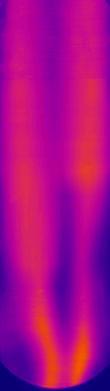
97 Fo=4 Fo=8 Fo=12 Fo=16 Fo=20 Fo=24 Fig Combustor wall temperature distributions associated with flame-acoustic interaction as a function of Biot number and Fourier number 81

98 Horizontal temperature profiles are sampled at four different Fourier numbers (Fo = 10, 15, 20, 25) and at 4, 7 and 10 inches in height of the combustor wall as shown in Fig Figures display these results, which can be compared against the results presented in Figs By normalizing the time scale for different wall thickness case with the appropriate conduction heat diffusion rate, various temperature profiles measured for different wall thickness were effectively collapsed into similar shapes at each Fourier number. This increases the confidence in the present approach of trying to determine the inner wall temperature distribution for the given window thickness. As described previously, the temperature profiles were symmetric for the baseline case, and asymmetric for the acoustically forced case. Also, the temperature difference between maximum and minimum is larger for the thinner wall (lower Biot number) case as shown in Figs This is thought to be the result of the actual diffusion rate being different in the y-direction (coming out of the wall) than in the x-direction (horizontal along the wall). The diffusion rate in the y-direction should be affected by local convection loss in the outer wall, which depends on the wall thickness. 82

99 1/32'' 1/16'' 1/8'' (a) 1/32'' 1/16'' 1/8'' (b) Fig Measurement of horizontal temperature distributions at three different heights: 4, 7 and 10 inches from the bottom line. (a) corresponding images for Fo = 20, (b) corresponding images for acoustic Fo = 20 83

100 (a) (b) (c) (d) (e) (f) (g) (h) Fig Horizontal temperature profiles at 4 inches from the bottom line: (a) temperature profiles for Fo = 10, (b) temperature profiles for acoustic Fo = 10, (c) temperature profiles for Fo = 15, (d) temperature profiles for acoustic Fo = 15, (e) temperature profiles for Fo = 20, (f) temperature profiles for acoustic Fo = 20, (g) temperature profiles for Fo = 25, (h) temperature profiles for acoustic Fo = 25 84

101 (a) (b) (c) (d) (e) (f) (g) (h) Fig Horizontal temperature profiles at 7 inches from the bottom line: (a) temperature profiles for Fo = 10, (b) temperature profiles for acoustic Fo = 10, (c) temperature profiles for Fo = 15, (d) temperature profiles for acoustic Fo = 15, (e) temperature profiles for Fo = 20, (f) temperature profiles for acoustic Fo = 20, (g) temperature profiles for Fo = 25, (h) temperature profiles for acoustic Fo = 25 85

102 (a) (b) (c) (d) (e) (f) (g) (h) Fig Horizontal temperature profiles at 10 inches from the bottom line: (a) temperature profiles for Fo = 10, (b) temperature profiles for acoustic Fo = 10, (c) temperature profiles for Fo = 15, (d) temperature profiles for acoustic Fo = 15, (e) temperature profiles for Fo = 20, (f) temperature profiles for acoustic Fo = 20, (g) temperature profiles for Fo = 25, (h) temperature profiles for acoustic Fo = 25 86

103 5.6 Inner Wall Temperatures After measuring the outer wall temperature distributions with three different thicknesses, the inner wall temperature distributions of the combustion chamber could be deduced from the results. The measurements corresponding to the three different wall thicknesses were combined with transient heat transfer analyses to calculate the inner wall temperature for the previously obtained flame characterization results. For this, it was assumed that the combustor flow conditions which determine the inner wall temperature would remain relatively independent of wall thickness. This allowed us to determine the temporal evolution of wall temperature profile as a function of the wall thickness and imposed boundary conditions. It may also be noted that the temperatures are in general higher for the acoustically forced case than for the baseline unforced case. Fig shows such dependence at two different instants. Three different wall thicknesses have been used to obtain the outer wall temperature as a function of time from the ignition. On the basis of these results, the analytical dependence on combustor wall thickness was compared, establishing the inner wall temperature as the zero-thickness limit. 87

104 (a) (b) Fig Combustor outer wall temperature as a function of combustor wall thickness and forcing conditions at certain instants after ignition 88

105 5.6.1 Comparison between Experimental and Analytical Results The expected temperature distributions in time are shown in Figs /32, 1/16, and 1/8 inches are the thicknesses of the outer wall temperatures measurement experiments. The temperature grows quickly with thinner walls. Fig shows the comparison between experimental and analytical temperature distributions in time for the baseline case. Fig. 5.26(b) displays the result of the whole combustor area, and fig. 5.26(c) shows the result of the local rectangle area as shown in Fig. 5.26(a). Fig displays the comparison between experimental and analytical temperature distributions for acoustic forcing case. As above, the results for the whole combustor are shown in Fig. 5.27(b), and fig. 5.27(c) shows the results of the local area. Good agreements were observed between experimental and analytical results for both of the baseline and acoustic forcing cases, and it is shown that temperature grows up much more quickly in the acoustic forcing case. 89

106 (a) (b) (c) Fig Comparison of analytical and experimental results for combustor outer wall temperature as a function of time (seconds) with baseline case. (a) corresponding image, (c) results of the whole combustor area, (c) results of the local area in the rectangle (a) (b) (c) Fig Comparison of analytical and experimental results for combustor outer wall temperature as a function of time (seconds) with acoustic forcing case. (a) corresponding image, (c) results of the whole combustor area, (c) results of the local area in the rectangle 90

107 5.6.2 Procedure of Extrapolating Wall Temperature Function Temperature on the outer wall is a function of δ, t, k,, h 1, h 3, T 1, T 3 : T w = f(x, y, t, δ, k, h 1, h 3, T 1, T 3 ) Instead of setting up an inverse heat transfer problem for inner wall temperature, some simplifying assumptions were established to extrapolate the inner wall temperature by exploiting its wall thickness dependence. One key assumption is that the combustor flow temperature is approximately independent of the wall thickness, in the range of time duration being investigated. This may be an acceptable simplification since the thermal output of the combustor is much greater than any heat transfer rate in this problem and the Biot numbers being considered are rather small. Under this setting, the inner wall temperature is the same as the outer wall temperature when the thickness becomes zero. The procedure is summarized in the five steps as follows: 1. Analytical Temperature Function : This analytical expression of combustor wall temperature was obtained as a function of wall thickness and time for small Biot numbers. ht1 h3t T(, t) ( h h ) 1 3 h 1( T1 T3 ) ( h1 h3 exp t ( h1 h3 ) 2c2 1 3 ) 2. Known Properties : Since the ambient flow and wall material properties are known, the number of unknowns can be reduced. This results in a family of curves T(δ,t) that depends on the combustor flow condition T 1,h 1. T w = f(x,y,t,δ,t 1,h 1 ) 91

108 3. Thin Wall Approximation : If we further assume that the combustor local flow conditions and heat transfer are not affected by the wall thickness, then the local wall temperature will depend only on time and wall thickness (that is for the given local T1 and h1.) T w = f(x,y,t,δ) 4. Experimental Data : From the measured data at various wall thicknesses, multiple boundary values can be established. Depending on local flow condition, there will be a family of curves such as this. at δ = δ 1, T w (x,y,t,δ 1 ) at δ = δ 2, T w (x,y,t,δ 2 ) at δ = δ 3, T w (x,y,t,δ 3 ) 5. Calibrate Inner Wall Temperature : For each location x, y, an analytical curve is selected that matches the obtained data the best (ex. Fig. 5.16). Then, in the limit as the thickness goes to zero, the temperature approaches the inner wall temperature. as δ 0, T inner wall = T w (x,y,t,δ=0) Obtaining Inner Wall Temperatures Finally, using the analysis, the inner wall temperature distribution with and without acoustic forcing were obtained and presented in Figs up to 15 seconds after the ignition. These inner wall temperature distributions are fairly agreeable. The structures are very close to the very thin wall cases (1/32 inch thickness) and the results of the distribution were as expected. The results showed that the maximum inner wall temperature reached nearly 1800K during the 92

109 short time. The temperature dispersion results should most closely follow that of the smallest Biot number case or the thinnest wall. For reducing the temperature uncertainty due to conduction along the tangential direction, the spatial resolution was reduced by averaging larger surface areas. Baseline case: 1s 2s 3s 4s 5s 6s 7s 8s 9s 10s 11s 12s 13s 14s 15s Fig Deduced inner wall temperature along with measured outer wall temperature distributions at select wall thicknesses and under various flow conditions for baseline cases 93

110 Acoustic Forcing case: 1s 2s 3s 4s 5s 6s 7s 8s 9s 10s 11s 12s 13s 14s 15s Fig Deduced inner wall temperature along with measured outer wall temperature distributions at select wall thicknesses and under various flow conditions for acoustic forcing cases 94

111 Similarly, the horizontal temperature profiles, including projected inner wall temperatures at three different heights (4, 7 and 10 inches from the floor), are presented in Figs , with Fig showing the measurement location. Here, different temperature scale and color were used because inner wall temperatures were much higher than measured outer wall temperatures. Each figure shows the results with baseline and acoustic forcing cases at three different times, which are 5, 10 and 15 seconds after the ignition. The temperature distributions of the inner wall temperatures show very similar patterns with the results of the outer wall temperature distributions. The projected inner wall temperatures were slightly increased and the temperature difference between inner wall and 1/32 inch thickness wall were lessened with the increase of time. In the same manner of previous results, the temperature profiles are symmetric for the baseline case and asymmetric for the acoustic case. 95

112 δ ~ 0'' 1/32'' 1/16'' 1/8'' (a) δ ~ 0'' 1/32'' 1/16'' 1/8'' (b) Fig Measurement of horizontal temperature distributions at three different heights: 4, 7 and 10 inches from the bottom line. (a) corresponding images for t = 10sec, (b) corresponding images for acoustic t = 10sec 96

113 (a) (b) (c) (d) (e) (f) Fig Horizontal temperature profiles at 4 inches from the bottom line: (a) temperature profiles for t = 5 sec, (b) temperature profiles for acoustic t = 5 sec, (c) temperature profiles for t = 10 sec, (d) temperature profiles for acoustic t = 10 sec, (e) temperature profiles for t = 15 sec, (f) temperature profiles for acoustic t = 15 sec 97

114 (a) (b) (c) (d) (e) (f) Fig Horizontal temperature profiles at 4 inches from the bottom line: (a) temperature profiles for t = 5 sec, (b) temperature profiles for acoustic t = 5 sec, (c) temperature profiles for t = 10 sec, (d) temperature profiles for acoustic t = 10 sec, (e) temperature profiles for t = 15 sec, (f) temperature profiles for acoustic t = 15 sec 98

115 (a) (b) (c) (d) (e) (f) Fig Horizontal temperature profiles at 4 inches from the bottom line: (a) temperature profiles for t = 5 sec, (b) temperature profiles for acoustic t = 5 sec, (c) temperature profiles for t = 10 sec, (d) temperature profiles for acoustic t = 10 sec, (e) temperature profiles for t = 15 sec, (f) temperature profiles for acoustic t = 15 sec 99

116 5.7 Instantaneous Flame Images The corresponding flow images for each wall thickness are also presented in Fig. 5.34, using the instantaneous OH* chemiluminescence obtained through the quartz window on the opposite side of the metal windows. These images were obtained to experimentally verify the state of the flames. With the thinnest wall (1/32 inch) case, there were some discrepancies for the acoustically forced conditions, as the acoustic forcing also interacted with the structure causing the thin metal window to vibrate. This resulted in damped acoustic-flame interaction. For all other cases, the observed flame-acoustic interaction was qualitatively identical to those from the earlier studies that used either 1.0-in thick quartz window or 0.5-in thick stainless steel window. Fig Comparison of flame-acoustic interaction under various thickness walls and combustor conditions 100

117 5.8 Uncertainty of the Measurements Measurement Uncertainty: The measurement error is significant for the assessment of measurement equipment accuracy. The evaluation of errors in infrared thermography is also necessary, especially the final values of measured temperature are obtained from the complex processing algorithm [Minkina 2004]. The infrared camera measurement model is defined as a function of five variables: T ob f (, T, T,, d) ob atm o where T ob is object temperature, ob is emissivity, T atm is atmosphere temperature, T o is ambient temperature, is humidity, and d is distance between object and IR thermography [Minkina and Dudzik 2009]. The actual emissivity value of the windows was experimentally determined by comparing the results with the thermocouple data. Here, atmosphere temperature ( T atm ), ambient temperature ( T o ) and humidity ( ) are continuously variable factors. In the IR thermography system, emissivity ( ob) value can be input to hundredths of a digit, and distance ( d ) value can be input to in tenths of a digit. This generates the uncertainties of digit errors. For the emissivity, the obtained emissivity value was 0.20, and this rounded-off number has ±2.5% of maximum digit uncertainty (0.005/0.20). This ±2.5% of emissivity (ε) uncertainty can affect only ±0.62% uncertainty of the measured temperature based on the relation between emissivity (ε) and temperature (T) : 1 T The actual distance ( d ) between combustor wall and IR thermography was 1.44 meters

118 However, the distance ( d ) value was input as 1.4 meters since the digit limitation of the system, and this creates about 2.78% of digit uncertainty (0.04/1.44). The influence of the uncertainty components associated with the distance ( d ), atmosphere temperature ( T atm ), ambient temperature ( T o ) and humidity ( ), are negligible to affect the apparent temperature of the object [Minkina 2004]. In addition, the used IR thermography (ThermaCAM SC3000) has its own measurement inaccuracy ranges which are ±1% below 150 C and ±2% above 150 C. In the experiments, the temperatures reached above 150 C very quickly, so the additional 2% of uncertainty should be considered. There are also two other factors to determine uncertainties : wall thickness (δ) and measured time (t). The maximum uncertainty of the stainless steel thin wall is about ±6.4% based on the minimum thickness (1/32'') and tolerance (±0.002'') of the metal. Finally, the uncertainty of the measured time is less than 1% based upon the period of the images (0.1 sec) and measuring time. Therefore, the measurement of total uncertainty can be affected by three major factors: apparatus (IR thermography), wall thickness (δ) and measured time (t). A basic Taylor series expansion was used to determine the total uncertainty, and the calculated total uncertainty is about 6.7%. f T IR f T IR 2 f 2 2 f t t The calculated maximum total uncertainty is about ±70 C. The tolerance of the thin wall thickness is the primary factor to determine the total uncertainty Revision of Temperature Range As mentioned in chapter 3, the temperature measurement device, IR thermometry, has four types of camera lenses, and each lens has different temperature ranges for the measurement 102

119 as shown in Table 3.1. Lens 3 was selected for the experiments because lens 3 covers the largest temperature range of interest. This camera lens can also measure the temperature out of the temperature ranges ( ºC). However, the discrepancies were observed in the range of temperatures below 100ºC, with increasing discrepancy at lower temperatures. For example, the lowest temperature that can be measured in this experiment was the room temperature (T ), which was 293K (20ºC), and this room temperature of 293K was recognized as 239K with this camera lens 3. This additional uncertainty affected the measurements in the beginning of the combustion test when the wall was below 100ºC. Fig. 5.35(a) displays one of the examples showing uncorrected measurements. This figure represents the horizontal temperature profile at 4 inches from the floor and 5 seconds after the ignition, and the temperatures were measured below a room temperature (293K) in the some of the area. Type of Lens Lens 1 Lens 2 Lens 3 Lens 4 Temp. Range - 20 ~ 80 (ºC) 10 ~ 150 (ºC) 100 ~ 500 (ºC) 350 ~ 1500 (ºC) Table 3.1 Temperature range of IR thermometry 103

120 (a) (b) Fig Example of the temperature uncertainty and revision at the 4 inches from the bottom line and 5 seconds after the ignition: (a) measured temperature distribution before revision, (b) temperature distribution after temperature revision 104

121 To solve this problem, the temperatures in the range of below 100ºC were shifted by the parabolic equation as shown in Fig which was calculated based on three boundary conditions. The basic quadratic parabolic equation with three unknowns (a, b, c) are expressed: T N a T 2 O b T O c (1) TN represents a new shifted temperature with the parabolic equation, and TO represents an old temperature which was measured by IR thermometry Boundary conditions: at T = 373K : a (373) 2 b (373) c 373 (2) O at T = 239K : a (239) 2 b (239) c 293 (3) O dtn at TO = 373K : 2a (373) b 1 (4) dt Solve equation (1) with three boundary conditions (2) - (4): a = , b = , c = Thus, T N T N O T N T 2 O T O (5) The expected temperature distribution (5) is shown in Fig A solid blue line is the shifted new temperature, and a dashed red line is an old measured temperature. 105

122 Fig Temperature revision by a quadratic parabolic equation: dashed red line - measured temperature by IR thermometry, solid blue line - revised new temperature 106

123 5.8.3 Deformation of Combustor Wall Integrity of the diagnostic window was affected at very high temperatures, and this could affect the experimental results. This phenomenon occurred most severely for the thinnest wall of the first location measurement because the temperature was highest at the first floor and the thinnest wall (1/32 inch) could easily be deformed. Fig shows some photographs of the warped and burnt metal window, taken after a test. (a) (b) Fig Example of the plate burning and warping 107

124 5.8.4 Temperature Aberration from Camera Lens In some experiments, dark spots were created on the temperature profiles due to the reflection of the camera lens onto the wall as shown in Fig. 5.38(a) because the temperatures of the reflected camera lens were measured degrees lower than the adjacent area. This problem was solved by eliminating any reflective surface on the metal window. After such treatment, the dark spots were eliminated as shown in Fig. 5.38(b). (a) (b) Fig Elimination of the dark spot on the wall temperature profile. Measurements taken (a) with reflective window surface, (b) with non-reflective surface 108