LUBRICATED TRANSPORT OF HEAVY OIL INVESTIGATED BY CFD THESIS SUBMITTED FOR THE DEGREE OF DOCTOR OF PHILOSOPHY AT THE UNIVERSITY OF LEICESTER

Transcription

1 LUBRICATED TRANSPORT OF HEAVY OIL INVESTIGATED BY CFD THESIS SUBMITTED FOR THE DEGREE OF DOCTOR OF PHILOSOPHY AT THE UNIVERSITY OF LEICESTER BY SALIM AL JADIDI JANUARY 2017

2 Abstract Heavy oil-water flow in horizontal pipes is studied by computational fluid dynamics (CFD) using the commercial CFD software ANSYS Fluent. Water-lubricated transport of heavy viscous oil core annular flow (CAF) is a promising technique for transporting heavy oil via horizontal pipes. This work investigates CAF numerically, using Large Eddy Simulation (LES). Its objectives are to gain an improved understanding of the behaviour of heavy oil flow through turbulent CAF in horizontal pipes and to examine the effectiveness and applicability of the LES. Heavy oil-waterair three-phase flow and heavy oil-water two-phase flow in horizontal pipe are simulated using ANSYS Fluent A relationship between the appearance of lubricated flow and the water inflow volume fraction is identified and related to oil fouling on the pipe wall. The rise in frictional loss is characterised and closely related to oil fouling on the pipe wall from the axial pressure gradient. The model predicts that fouling can be minimized by increasing the water flow. It is found that the water phase affects the behaviour of the CAF and the axial pressure drop. It was observed that greater stability in the CAF leads to a reduction in the axial pressure drop to a value close to that for a water flow. The impact of temperature on three-phase heavy oil-water- air flow in a horizontal pipe is affected by gravity. It has been observed that the air phase and changes in the temperature influence the stability of annular flow and the axial pressure drop. Some results made during this study are validated with reference experimental and numerical results from literature and shown to be in reasonably good agreement. I

3 Acknowledgements I would like to express my thanks and gratitude to my supervisor Dr. Shian Gao for all of his efforts, guidance, support and assistance over the past years to the completion of the present work. He is always ready to support me for any discussions related to my study over the past years. His support contributed to completing the project successfully. I would also like to thank my cosupervisor Dr. Andrew McMullan for his support. Special thanks go to Dr. Aldo Rona for all his valuable discussions and his feedback. As well, I would like to thank all my colleagues in the thermo-fluids group for their help. My appreciation goes to my sponsor Ministry of Manpower in Sultanate of Oman for their help and financial support which is highly appreciated. Finally, my grateful and special thanks to my family, mother, brothers and sisters for their love, helps and supports. They gave me an inspiration and encouragement to obtain a higher educational degree. II

4 Table of contents Abstract... I Acknowledgements... II Table of contents... III List of figures... VIII List of abbreviations... XVI Nomenclatures... XVII Greek letters... XVIII Chapter 1 Introduction Introduction and background Motivation behind conducting this study Thesis aims and objectives Thesis outline... 7 Chapter 2 Literature review Introduction and background Heavy crude oil industrial background (transportation) Water-lubricated heavy oil transport applications Multiphase and two-phase liquid-liquid flow in heavy oil transportation Effect of viscosity Fouling and restart Some notations in heavy crude oil-water flow LES of turbulent flows Chapter 3 Numerical modelling of multiphase flows Fundamentals of CFD Multiphase flow with CFD Standard κ-ε model κ-ω SST model III

5 3.5 LES model SGS modelling Eddy viscosity model Smagorinsky-Lilly model Numerical simulation of transport equations Review of numerical solution methods The discretized transport equations SIMPLE algorithm PISO algorithm Errors sources in CFD simulations Chapter 4 CFD simulation of heavy oil water flows through sudden contraction and expansion pipes Introduction and background Objectives CFD simulation model Methodology and model development Governing equations for flow modelling Numerical method Interface treatment Physical models Geometry creation Simulation setup Initial conditions and boundary conditions Velocity inlet-boundary condition Boundary condition at pipe outlet Boundary conditions at pipe wall Time-marching scheme Solution setup Results and discussion Sudden expansion flow predictions IV

6 Sudden contraction flow predictions Development of core annular flow through a sudden contraction Core annular flow through the sudden expansion and oil fouling Hydrodynamic study Summary Chapter 5 Heavy oil-water flow through sudden contraction and expansion pipes fittings using LES Motivation and background Objectives Numerical formulation and methodology CFD simulation of LES for CAF in the contraction and expansion of horizontal pipes LES Methodology and model development Governing equations and numerical methods for flow modelling Governing equations Numerical method Near-wall treatment of the LES model Geometry and mesh generation Discretization result systems and computational set-up Results and discussion Sudden expansion flow predictions Sudden contraction flow predictions Development of the core annular flow through a sudden contraction Core annular flow through the sudden expansion and oil fouling Hydrodynamic study Summary Chapter 6 CFD simulation of heavy oil water flow CAF in horizontal pipe using the LES model Introduction Objectives V

7 6.3 CFD simulation setup and model development and LES approach Introduction Physical model Numerical model LES model Near-wall treatment for LES model Implementation of the numerical model Initial conditions and boundary conditions Simulation setup Simulations Results and discussion Effect of the domain initialization method Effect of the oil-water interface reconstruction method Effect of the sub-grid-scale model Comparison simulation results with experimental flow study Summary Chapter 7 CFD simulation of heavy oil-water-air flow through a horizontal pipe using an LES model Objectives Numerical formulation and methodology CFD Simulation of LES for CAF in the horizontal pipe VOF model Model development and LES approach Physical model Governing equations Numerical methodology Boundary conditions Interface treatment and near-wall treatment of the LES model Computational set-up Results and discussion VI

8 Impact of the air phase Impact of temperature change Impact of temperature and of the presence of air on the pressure drop Temperature profiles fields Summary Chapter 8 Conclusion and recommendation Conclusion Recommendation References VII

9 List of figures Figure 1-1: Schematic of core annular flow in a horizontal pipe... 3 Figure 1-2: Schematic of core annular flow in horizontal pipe contraction...3 Figure 1-3: Schematic of core annular flow in horizontal pipe expansion...4 Figure 2-1: Heavy oil transportation methods Figure 2-2: Scheme for a staggered mesh in two dimensions Figure 2-3: Computational cell and arrangement of variables in the X-momentum equation Figure 3-1: Schematic of the computational domain spatial discretization Figure 4-1a: Meridional plane computational domain cross-section of three dimensional CFD model of sudden expansion horizontal pipe Figure 4-1b: Meridional plane computational domain cross-section of three dimensional CFD model of sudden expansion horizontal pipe Figure 4-2a: Meridional plane computational domain cross-section of three dimensional CFD model of sudden contraction horizontal pipe Figure 4-2b: Meridional plane computational domain cross-section of three dimensional CFD model of sudden contraction horizontal pipe Figure 4-3: 3D structured grid for Expansion Figure 4-4: 3D structured grid for contraction Figure 4-5: Oil volume fraction contours for different computational mesh sizes. Red denotes water and dark blue denotes oil Figure 4-6: Velocity magnitude on the meridional plane Figure 4-7: Vectors coloured by the velocity magnitude on the meridional plane Figure 4-8: Pathlines coloured by the velocity magnitude on the meridional plane Figure 4-9: Velocity magnitude on the meridional plane Figure 4-10: Vectors coloured by the velocity magnitude on the meridional plane Figure 4-11: Pathline coloured by the velocity magnitude on the meridional plane Figure 4-12: Development of core flow with time through the contraction of figure 4-2: U so = 0.6 m/s and U sw = 0.3 m/s Colour iso-levels of water volume fraction Figure 4-13: Development of core flow by increasing U sw from 0.3 m/s to 0.8 m/s at constant U so of 0.6 m/s. Colour iso-levels of velocity magnitude VIII

10 Figure 4-14: Colour iso-levels of water volume fraction predicted at different inflow conditions through the sudden expansion of figure 4-1. κ-ω SST model. Red denotes water and blue denotes oil Figure 4-15: Colour iso-levels of water volume fraction predicted at different inflow conditions through the sudden expansion of figure 4-1. κ-ε model. Red denotes water and blue denotes oil Figure 4-16: Axial distribution of total pressure drop Figure 4-17: Axial distribution of static pressure drop Figure 4-18: Colour iso-levels of velocity magnitude at L/D = -10, upstream of the sudden contraction. U so = 0.6 m/s and U sw = 0.3 m/s Figure 4-19: Colour iso-levels of velocity magnitude at L/D = -10, upstream of the sudden expansion. U so = 0.6 m/s and U sw = 0.8 m/s Figure 4-20: Radial profiles of velocity at different axial positions Figure 4-21: Radial profiles of velocity at different axial positions Figure 4-22: Time averaged values of mean volume fraction of oil along the axis Figure 4-23: Time averaged values of mean volume fraction of oil along the axis Figure 4-24: Axial distribution of total pressure drop Figure 4-25: Axial distribution of static pressure drop Figure 4-26: Time averaged values of mean volume fraction of oil along the axis Figure 4-27: Time averaged values of mean volume fraction of oil along the axis Figure 4-28: Radial profiles of velocity at different axial positions Figure 4-29: Radial profiles of velocity at different axial positions Figure 4-30: Colour iso-levels of water volume fraction at axial planes L/D 7 at different times; U so = 0.6 m/s and U sw = 0.3 m/s. κ-ε model of the sudden contraction of figure 4-2. Red denotes water and blue denotes oil Figure 4-31: Colour iso-levels of water volume fraction across axial planes through the contraction of figure 4-2 at t = 1.12 sec; U so = 0.6 m/s, U sw = 0.3 m/s. κ-ε model. Red denotes water and blue denotes oil IX

11 Figure 4-32: Colour iso-levels of water volume fraction across axial planes through the sudden expansion of figure 4-1 at = 1.02 sec; U so = 0.6 m/s and U sw = 0.3 m/s. κ-ε model. Red denotes water and blue denotes oil Figure 4-33: Colour iso-levels of water volume fraction across axial planes through the sudden expansion of figure 4-1 at t = 1.02 sec; U so = 0.6 m/s and U sw = 0.3 m/s. κ-ω SST mode of the sudden expansion. Red denotes water and blue denotes oil Figure 4-34: Colour iso-levels of water volume fraction across planes through the sudden expansion of figure 4-1 at t = 1.02 sec; U so = 0.6 m/s and U sw = 0.6 m/s. κ-ω SST model. Red denotes water and blue denotes oil Figure 4-35: Colour iso-levels of water volume fraction across axial planes through the sudden expansion of figure 4-1 at t = 1.02 sec; U so = 0.6 m/s and U sw = 0.8 m/s. κ-ε model of the sudden expansion of figure 4-1. Red denotes water and blue denotes oil Figure 5-1: Colour iso-levels of velocity magnitude by velocity magnitude across the meridionall plane Figure 5-2: Vectors coloured by velocity magnitude across the meridional plane Figure 5-3: Pathlines coloured by velocity magnitude across the meridional plane Figure 5-4: colour iso-levels of velocity magnitude across the meridional plane Figure 5-5: Vectors coloured by velocity magnitude across the meridional plane Figure 5-6: Pathline by velocity magnitude along meridional plane Figure 5-7: Development of core flow with time through the sudden contraction. U so = 0.6 m/s and U sw = 0.3 m/s. Colour iso-levels of water volume fraction Figure 5-8: Colour iso-levels of velocity magnitude across the meridional plane. LES at t =1.5 seconds through a sudden contraction Figure 5-9: Colour iso-levels of velocity magnitude across the meridional plane through a pipe with sudden expansion. LES at t =1.2 seconds at different inflow oil-water interface surface velocity combinations. Red denotes water and blue denotes oil Figure 5-10: Colour iso-levels of velocity magnitude through a sudden expansion modelled by LES at t = 1.2 seconds for a range of U sw = 0.6 m/s to 1.0 m/s at constant U so = 0.6 m/s Figure 5-11: Axial distribution of total pressure drop Figure 5-12: Axial distribution of total pressure drop X

12 Figure 5-13: Colour iso-levels of velocity magnitude predicted by LES at U so = 0.6 m/s, U sw = 0.3 m/s, L/D = -10, upstream of the sudden contraction at t =1.15 seconds Figure 5-14: Colour iso-levels of velocity magnitude predicted by LES at U so = 0.6 m/s, U sw = 0.8 m/s, L/D = -10, upstream of the sudden expansion at 1.2 seconds Figure 5-15: Radial profiles of velocity at different axial positions Figure 5-16: Radial profiles of velocity at different axial positions Figure 5-17: Time averaged values of mean volume fraction of oil along the axis Figure 5-18: Time averaged values of mean volume fraction of oil along the axis Figure 5-19: Colour iso-levels of water volume fraction at axial planes L/D = 7 at different times, U so = 0.6 m/s, U sw = 0.3 m/s. LES through the pipe sudden contraction. Red denotes water and blue denotes oil Figure 5-20: Colour iso-levels of water volume fraction α w through the pipe sudden contraction predicted by LES at t = 1.15 sec; U so = 0.6 m/s, U sw = 0.3 m/s. Red denotes water and blue denotes oil Figure 5-21: Colour iso-levels of water volume fraction α w through the pipe sudden expansion predicted by LES at t = 1.15 sec; at different axial locations, U so = 0.6 m/s, U sw = 0.3 m/s. Red denotes water and blue denotes oil Figure 5-22 Colour iso-levels of water volume fraction α w through the pipe sudden expansion predicted by LES at t = 1.15 sec; U so = 0.6 m/s, U sw = 0.8 m/s. Red denotes water and blue denotes oil Figure 5-23: Colour iso-levels of water volume fraction α w through the pipe sudden expansion predicted by LES at t = 1.15 sec; U so = 0.6 m/s, U sw = 0.6 m/s. Red denotes water and blue denotes oil Figure 5-24: Colour iso-levels of water volume fraction α w through the pipe sudden expansion predicted by LES at t = 1.15 sec with U sw = 0.8 m/s U so = 0.8 m/s. Red denotes water and blue denotes oil Figure 5-25: Variation of core thickness with superficial velocity, contours of water volume fraction from CFD Figure 5-26: Variation of core thickness with superficial velocity contours of water volume fraction from CFD simulations; Red denotes water and yellow denotes oil XI

13 Figure 6-1: Schematic of the flow domain and dimensions of a three dimensional CFD model, and details of water and oil inlet sections Figure 6-2: 3D unstructured grid at the inlet and outlet regions Figure 6-3: Development of core flow with simulation time. (a) Domain initialization from the water inflow (HV-3); (b) Domain initialization from the oil inflow (HV-3-2). Colour iso-levels of the oil volume fraction predicted by LES. Red denotes oil and blue denotes water Figure 6-4: Colour iso-levels of oil volume fraction α w to predicted by LES with (a) The CICSAM scheme (HV-1-2) and (b) The Geo-Reconstruction (HV-1). Red denotes oil and blue denotes water Figure 6-5: Colour iso-levels of oil mass fraction predicted by LES at t = seconds with different SGS models and comparison with experimental flow by Charles et al. [36]. In experiment, the black illustrates water and white with dots inside illustrates oil. Red denotes water and blue denotes oil. Pressure gradient from different SGS models versus experiment, with percentage differences Figure 6-6: Axial plane distribution of turbulent quantities predicted by different SGS models at L/D = abd t = seconds. (a) Smagorinsky-Lilly model (LV-3-2); (b) WALE model (LV-3-3); (c) WMLES (LV-3-4); (d) WMLES S-Omega model (LV-3) Figure 6-7: Comparison of predicted CAF by LES and the Smagorinsky-Lilly SGS model at t = seconds with experiment from Charles et al. [36]. In Charles et al. [36]; the black denotes water and the white with dots inside denotes oil. Colour iso-levels of oil volume fraction from CFD. Red denotes oil and blue denotes water Figure 6-8: Comparison of predicted CAF by LES and the Smagorinsky-Lilly SGS model at t = seconds with five different superficial oil and water velocity combination. colour iso-levels of oil volume fraction. Red denotes water and blue denotes oil Figure 6-9: Colour iso-levels of oil volume fraction across four axial planes predicted for cases at (a) HV-2 and t = sec, (b) HV-7 and t = sec, (c) HV-7 and t = sec and HV- 8 and t = sec. Red denotes water and blue denotes oil Figure 6-10: Oil phase volume fraction and axial velocity profiles of low viscosity CAF at various axial positions. Predictions by LES with the Smagorinsky-Lilly model at t = 10.2seconds XII

14 Figure 6-11: Sub-grid-scale eddy viscosity μ t and effective eddy viscosity of low-viscosity CAF at various axial positions. Predictions by LES with the SGS model by Smagorinsky-Lilly model at t = 10.2 seconds Figure 6-12: Oil phase volume fraction and axial velocity profiles of high viscosity oil and water CAF at various axial positions. Predictions by LES with the SGS model by Smagorinsky at t = seconds Figure 6-13:Sub-grid-scale eddy viscosity and effective eddy viscosity of high-viscosity CAF at various axial positions.. Predictions by LES with the SGS model by Smagorinsky at t = seconds Figure 7-1: Schematic of the flow domain and dimensions of a three dimensional CFD, and details of water and oil-air inlet sections Figure 7-2: Radial profiles of superficial velocity for oil in the heavy oil-water flow at various axial positions. LES at time t = seconds Figure 7-3: Radial profiles superficial velocity of the water in the heavy oil-water phase at various axial positions. LES at time t = seconds Figure 7-4: Radial profiles superficial velocity of the oil in the heavy oil-water-air flow at various axial positions. LES at time t = 14.3 seconds. T = K Figure 7-5: Radial profiles superficial velocity of the oil in the heavy oil-water-air flow at various axial positions. LES at time t = 14.7 seconds. T = K Figure 7-6: Radial profiles superficial velocity of the oil in the heavy oil-water-air at various axial positions. LES at time t = 14.1 seconds. T = K Figure 7-7: Radial profiles superficial velocity of the oil in the heavy oil-water-air flow at various axial positions. LES at time t = seconds. T = K Figure 7-8: Colour iso-levels of oil volume fraction at T = K in heavy oil-water-air LES at various axial flows. LES at time t = 14.3 seconds. Red denotes oil and blue denotes water 189 Figure 7-9: Colour iso-levels of oil volume fraction at T = K in heavy oil-water LES at various axial flows. LES at time t = 14.7 seconds. Red denotes oil and blue denotes water Figure 7-10: Colour iso-levels of oil volume fraction at T = K in heavy oil-water-air LES at various axial flows. LES at time t = 14.1 seconds. Red denotes oil and blue denotes water. 190 XIII

15 Figure 7-11: Colour iso-levels of il volume fraction at T = K in heavy oil-water-air LES at various axial flows. LES at time t = seconds. Red denotes oil and blue denotes water Figure 7-12: Predicted radial profiles of oil superficial velocity at various temperatures at X = 1000 mm and Z = 0. LES at time t = 14.7 seconds, Heavy oil-water-air simulations Figure 7-13: Colour iso-levels of predicted oil volume fraction for various temperatures, on an axial plane at 1000 mm from the entrance. LES of oil-water-air flow at t = 14.7 seconds. Red denotes oil and blue denotes water Figure 7-14: Radial profiles of oil temperature at four axial positions (X) along the pipe, at Z = 0 m and T = K Figure 7-15: Radial profiles of water temperature at four axial positions (X) along the pipe, at Z = 0 m and T = K Figure 7-16: Radial profiles of oil temperature at four axial positions (X) along the pipe, at Z = 0 m and T = K Figure 7-17: Radial profiles oil temperature at four axial positions (X) along the pipe, at Z = 0 m and T = K Figure 7-18: Radial profiles of oil temperature at four axial positions (X) along the pipe, at Z = 0 m and T = K Figure 7-19: Oil temperature field ( K) in the YZ plane at X = 1000 mm, along the pipe Figure 7-20: Water temperature ( K) field in the XY plane along the pipe Figure 7-21: Oil temperature field ( K) in the YZ plane at X = 1000 mm, along the pipe Figure 7-22: Oil temperature field ( K) in the YZ plane at X = 1000 mm, along the pipe Figure 7-23: Oil temperature field ( K) in the YZ plane at X = 1000 mm, along the pipe XIV

16 List of tables Table 4-1: Fluid phases physical properties Table 4-2: Horizontal pipes geometries dimensions Table 4-3: Outlet conditions Table 4-4: Wall boundary conditions Table 4-5: ANSYS Fluent solution control method Table 4-6: Computational setup...67 Table 5-1: ANSYS Fluent solution control method Table 5-2: Computational setup Table 6-1: Computational setup Table 6-2: ANSYS Fluent solution control method Table 6-3: Fluid Properties Table 7-1: Thermo-physical Properties of the three fluid phases (25 C) used in the present study Table 7-2: Horizontal pipe geometry dimensions Table 7-3: Equations of the three fluid phases used to obtain viscosity in the present study Table 7-4: ANSYS Fluent solution control method Table 7-5: Computational setup Table 7-6: Pressure drop as a function of the temperature of the mixture at the inlet of the pipe XV

17 List of abbreviations API American petroleum institute CAF Core annular flow CFD Computational fluid dynamics 3-D Three-dimensional DNS Direct numerical simulation FVM Finite volume method HV High viscosity LES Large eddy simulation L Laminar LV Low viscosity L / D Length-diameter ration NSE Navier-Stokes equation O Oil OW Oil-water interface PISO Pressure implicit split operator PRESTO! Pressure staggering option QUICK Quadratic upstream interpolation of convective kinematics RANS Reynolds-averaged Navier-Stokes SIMPLE Semi implicit method for pressure linked equations SST Shear stress transport S Superficial VOF Volume of fluid W Water XVI

18 Nomenclatures Symbols A Pipe cross-sectional area, m 2 A o Areas occupied by oil phase, m 2 A w Area occupied by water phase, m 2 C k C o C p C w D Courant number Roughness coefficient of effective wall Oil volume fraction Specific heat capacity, J. kg 1.K 1 Water volume fraction Pipe diameter, m F Force per unit mass, m/s 2 F Force per unit volume, kg/m 2 s 2 f Friction factor g Gravity constant, m/s 2 H o Holdup of oil phase H w h Holdup of water phase Oil and water holdup ratio, h= H w/h o C w /C o k Specific kinetic energy of turbulence, m 2 /s 2 ε Effective relative wall roughness P Pressure, N/m 2 ΔP Pressure drop, Pa Q Flow rate, m 3 /s Q o Oil flow rate, m 3 /s Q w Water flow rate, m 3 /s XVII

19 R Re R sk S S T T t U so U sw u Pipe radius, m Reynolds number Skewness Source term Total heat sources W.m 3 Temperature, K Time, s Superficial velocity of oil phase, m/s Superficial velocity of water phase, m/s Velocity, m/s V Volume, m 3 /s x, y, z Coordinates m X, Y, Z Dimensionless coordinates Greek letters ε o ε w Average in situ volume fraction of oil Average in situ volume fraction of water ε Turbulence dissipation rate, m 2 /s 3 Г λ μ μ f μ t μ o μ w Diffusion coefficient Friction factor Molecular viscosity, kg m 1 s 1 Friction coefficient Turbulent viscosity, k kg m 1 s 1 Viscosity of oil phase, kg m 1 s 1 Viscosity of water phase, kg m 1 s 1 ρ Density, kg/m 3 XVIII

20 ρ o Oil density, kg/m 3 ρ w Water density, kg/m 3 α α o α w σ Volume fraction Oil volume fraction Water volume fraction Interfacial tension, N/m τ Shear stress, N/m 2 τ w Wall shear stress, N/m 2 ϑ φ Relaxation factor An intensive property of the flow ω Specific turbulence dissipation rate, 1/m XIX

21 Chapter 1 Introduction 1.1 Introduction and background The petroleum industry is one of the main participants in the energy sector in the world. The greater demand for light oil reserves over past decades has led to their depletion. As a result, heavy oil is increasingly a topic of interest, receiving considerable attention with regard to its efficient transportation. High viscous oil (heavy crude oil) is believed to be the future of sustainable oil production globally, but it remains unclear how best it can be exploited, as observed by Lyman et al. [92]. Sharing knowledge and the latest technology will be beneficial for all players in the oil industry, as heavy oil extraction, transportation and utilization poses a unique set of challenges. Technology providers have begun heavily investing in the development of new technologies to ensure heavy crude oil can be a commercial alternative to light oil for the oil industry (Saniere et al. [136] and Pospisil [120]). Heavy crude oil reserves have grown in recent years, and as a result, many scientists and researchers have become interested in the potential of heavy crude oil as an appropriate and suitable substitute for light oil, as well as a reasonable solution to meet the growing global demand for energy (Urquhart [150]). As observed by Martínez-Palou et al. [95], this had led to an increase in demand and widespread use of large amounts of heavy crude oil; growth in usage helps to drive technological improvements, which can then help countries and companies to extract and transport large amounts of heavy crude oil. Despite the large quantity of productive heavy crude oil reserves, the transport of heavy crude oil is complex and costly, due to its high viscosity. Due to this characteristic, heavy crude oil requires a large amount of power to pump it. At present, different methods are employed to transport heavy oil from the production field to refineries and on to the marketplace. Although many other options are available, pipelines are the safest and most efficient and financially viable means of transporting heavy oil (Martínez-Palou et al. [95] and Guevara et al. [62]). This method of transportation requires the use of specialized fittings to pump the heavy oil along pipelines. However, pipeline transportation in general is very expensive and in some cases is impossible to implement, due to difficult terrain and the high viscosity of oil. Thus, to facilitate the transportation of heavy crude oil, it is more important to 1

22 study how best to transport a viscous fluid towards providing a technical and commercially viable solution. This problem has been addressed in recent years. Different techniques and technologies have been proposed to reduce the viscosity of the heavy oil. Conventional methods are heating, blending with either light oil or kerosene or other additives, using steam as an adjunct and forming oil-in-water emulsions. However, these conventional methods have limitations and current solutions are costly. Additional details relating to conventional methods are given in chapter 2. The current difficulties with these established techniques have prompted scientists and researchers to search for alternative solutions for the transportation of highly viscous fluids. One promising solution is a new technology that provides water-lubricated transport of heavy oil, termed core annular flow (CAF). CAF is a technique whereby the water flows into the area of high shear at the wall of the horizontal pipe lubricating the flow. More details regarding the CAF technique are given in chapter 2. Alboundwarej et al. [6], Anand et al. [8], Arirachakaran et al. [15], Bannwart et al. [21], Brauner et al. [30] and Joseph et al. [77] have provided excellent reviews of oil-water flow techniques, evaluating different flow systems. Currently, CAF is a popular method ensuring safety and cost effectiveness, remedying some of the limitations of conventional approaches; researchers have found CAF to be a highly successful method for use in pipelines to transport very viscous oil (Bai et al. [17], Bannwart [20], Bensakhria et al. [24], Ghosh et al. [59], Herrera et al. [66], Joseph et al. [76], Kiyoung and Haecheon, [82], Lo and Tomasello [90], Oliemans and Ooms [104] and Rodriguez et al. [125] ). When applied, CAF technology uses multiphase flow, which can be either a liquid-liquid-gas flow or a liquid-liquid flow. The present study investigates the transportation of heavy crude oil using CAF technology as a suitable option to reduce wall friction in pipe flows. It studies the effects of the axial pressure gradient and of temperature. It also explores how best to prevent oil fouling at the horizontal pipe wall, reducing the amount of power required, and thereby the transportation cost. In oil-water CAF, friction at the pipe wall reduces because of the flow of water. This reduces the axial pressure drop along the pipeline. This method can reduce the pumping energy required for a given mass of oil compared to the conventional transportation techniques mentioned above. CAF describes the flow of a high viscosity liquid surrounded by a low viscosity liquid annular layer, through horizontal 2

23 pipes (see figure 1-1 for horizontal pipe, and figure 1-2 and 1-3). In the case considered, the high viscosity liquid is heavy oil and the low viscosity liquid is water. Among researchers, this method is indicated to be the best and most successful for the pipeline transport of heavy crude oil. The present study scrutinizes the behaviour of CAF by computational fluid dynamics (CFD), using the κ-ω SST model, which is presented in chapter 4 and a large eddy simulation (LES) model, which is presented in chapters 5, 6 and 7. Figure 1-1: Schematic of core annular flow in a horizontal pipe. Figure 1-2: Schematic of core annular flow in horizontal pipe contraction. 3

24 Figure 1-3: Schematic of core annular flow in horizontal pipe expansion. For liquids, the effect of a change in pressure is relatively smaller when compared to the effect of a change in temperature, however, large axial pressure gradient and shear stress at the wall tend to occur with high viscosity oil. At Reynolds numbers less than 100, friction can become significant. CAF technology tends to reduce friction, which reduces the axial pressure gradient. The most essential characteristic of the CAF method is that it does not change and modify the viscosity of the heavy oil, but it changes the flow type and decreases friction from heavy oil transport. This reduction in friction leads to decrease in the axial pressure drop and, therefore, to decrease in pumping power. In the oil pipeline industry, there has been limited use of oil-water CAF transport. Its widespread adoption could reduce the average pressure drop in the pipeline, however, the more complex flow pattern can also cause problems and transport difficulties specifically, these techniques are sensitive to fouling, which increases the wall friction at the pipes, the shear stress at the wall and the axial pressure drop. The present study will attempt to characterize the behaviour of water-heavy crude oil flow through CAF in a constant diameter pipe and where it encounters a sudden change in the cross-section, through either a contraction or an expansion of the horizontal pipe. Several simulations will be 4

25 performed during this study to understand the CAF through these three types of wall geometries. Highly viscous fluids will be used to highlight the influence of viscosity on the flow, specifically on fouling, wall friction, wall shear stress, and pressure drop characteristics. These CFD investigations will help understand the variations in the axial pressure gradient and in the wall shear stress with the velocities of oil and water, as well as with the oil volume fraction. In addition, the study investigates the effect of temperature. 1.2 Motivation behind conducting this study Past studies covered many aspects of water lubricated transport in two phase liquid-liquid flow (oil and water) using CFD simulations with a κ-ε model and κ-ω SST model (Bannwart [20], Bensakhria et al. [24], Ghosh et al. [59], Herrera et al. [66], Jing Shi [74], Joseph et al. [76] and Das et al. [79] ). However, LES has not been reported. Therefore this study will attempt to describe the water lubricated transport of three phase liquid-liquid-gas flow (oil, water and air) and two phase liquid-liquid flow (oil and water) with an LES. In this context, this study will evaluate the influence of temperature and the of the water phase on the thermo-hydrodynamics of the heavy oil-water flow in a horizontal pipe. 1.3 Thesis aims and objectives The main aim of the study is to model the behaviour of heavy oil and water in horizontal pipes. It aims to develop a suitable CFD model for a three-phase liquid-liquid-gas CAF through a horizontal pipe and a two-phase liquid-liquid CAF through a sudden contraction and an expansion in horizontal pipes. A further objective was to study the influence of temperature and of the water phase on the thermo-hydrodynamics characteristics of two-phase heavy oil-water flow in a horizontal pipe, under the impact of gravity. At the end of the work, new techniques will be developed to obtain accurate phase predictions in the CAF. To attain the main objectives of this study, sub-aims detailing areas of work were established as follows: Reviewing three-phase liquid-liquid-gas flow models (heavy oil, water and air flow) and two-phase liquid-liquid flow models (heavy oil-water-air flow); 5

26 Evaluating three-phase models (heavy oil-water-air) and two-phase models (heavy oilwater), as available in the literature; Determining an appropriate approach for modelling heavy oil-water flow to achieve new information and data; Collating information from previous modelling studies to create a large database for analysis; Conducting three dimensional CFD modelling for heavy oil-water flow utilizing the CFD package ANSYS Fluent; Investigating the strength and capability of three and two phase CFD models as developed in ANSYS Fluent; Evaluating the VOF method by computing three phase liquid-liquid-gas in CAF and two phase liquid-liquid in CAF; Evaluating the different results obtained using these two numerical modelling methods; Analysing the flow predictions and comparing these with previously published studies and developing the understanding of flow features; Gaining cross-sectional flow data to improve knowledge concerning flow features and characteristics; Developing a suitable semi-empirical model for predicting the head loss through CAF, based on the CFD results. The following working plan was thus proposed: Review the previous literature concerning CAF and specifically on CAF simulations. This includes an investigation and verification of the sudden contraction and expansion model in a horizontal pipe. To attain the desired results, the following procedure was identified: I. To conduct a literature review on CAF, including an investigation of different experimental and numerical modelling techniques; II. To design a model geometry to develop a CAF regime for use with different horizontal pipes; 6

27 III. To develop and design a suitable CFD model in 3D by ANSYS Fluent which can be used in pipes with different horizontal diameters; IV. To develop a model with the ability to calculate the volume fractions in two phase liquidliquid flow; V. To test the performance of the κ-ε model, κ-ω SST model and the LES model with threephase liquid-liquid-gas flow (oil, water and air) and two-phase liquid-liquid flow (oil and water); VI. To develop post-processing techniques, to calculate the film velocity distribution in the oil and in the water phases; VII. To develop a semi-empirical model to predict head loss due to (fouling, wall friction, pressure drop, velocities, and volume fractions of oil and water phases, and the impact of temperature) for CAF in a horizontal pipe, based on CFD predictions. VIII. To understand the dependence of the axial pressure gradient and wall shear stress on the fluid velocities of oil and water, and to understand the influence of temperature. 1.4 Thesis outline This thesis is organized into eight chapters describing the work completed and the relationship between the content and objectives presented in section 1.3. A brief background and the rationale for carrying out this work have been discussed here, in Chapter 1. Chapter 2 presents a literature review detailing the industrial background of heavy oil transport and explaining previous studies on this topic. It then explains popular CFD modelling approaches for three and two phase flows and describes the flow regimes of three-phase liquid-liquid-gas and two-phase liquid-liquid flow in horizontal pipes. Chapter 3 describes the numerical methods used in this study to model the CAF for transporting heavy crude oil. 7

28 Chapter 4 describes the numerical models of two-phase liquid-liquid CAF of heavy oil-water. Constant section, contracting and expanding horizontal pipes CAF models are obtained with the κ-ε model and the κ-ω SST model. The computational domain geometry, grid arrangements, selection of flow solver type, and the boundary conditions employed in this work are presented. The simulation results are discussed and compared against reference predictions by Das et al. [79] Chapter 5 presents LES of heavy oil-water CAF in contracting and expanding horizontal pipes. The numerical procedure, grid arrangements, discretization of governing equations and the boundary conditions employed in this work are presented. Additionally, the chapter discusses the simulation results and evaluates these against the reference numerical predictions by Das et al. [79] Chapter 6 presents high viscosity two phase heavy oil-water CAF flow behaviour in horizontal pipes using LES. Chapter 7 described the impact of temperature in heavy crude oil- water- air CAF flow using the LES model. The chapter explains the simulation results against reference numerical results by Gadelha et al. [14] Chapter 8 summarizes the conclusions arising from the study and offers suggestions and recommendations for future work. 8

29 Chapter 2 Literature review 2.1 Introduction and background CAF for the transportation of heavy viscous oils is a technique whereby water flows as an annular film into the cross-sectional area of high shear strain rate at the pipe wall, allowing oil to flow in the core area, these by lubricating the flow of oil. As the oil does not typically interact with or touch the wall, the wall shear stress is practically identical to the shear stress produced by the flow of water through the same pipe. If the pressure produced by a pump is balanced by the wall shear stresses from the water, then a lubricated flow requires a pressure similar to that needed when pumping water alone, regardless of the viscosity of the oil. Researchers have conducted many investigations into CAF; e.g. Al-Awadi [5], Andrade et al. [10], Balakhrisna et al. [18], Beerens [23], Gosh et al. [60], Lovick and Angeli, [91], Ooms et al. [106, 108 and 109], Raghvendra et al. [121] and Trallero et al. [145]. The literature encompasses numerous aspects, which integrate, customize and incorporate models for levitation, as well as empirical studies and experimental investigations into energy efficiency in relation to different flow types, empirical correlations providing the pressure drop against mass flux, stability studies, and industrial applications of CAF. This chapter provides essential knowledge about CFD for three phase heavy oil-water-air flow and two phase heavy oil-water flow to explain the simulation procedures and to enhance the understanding of the simulation results provided in this study. 2.2 Heavy crude oil industrial background (transportation) Heavy crude oil is labelled as heavy if its viscosity is higher than that of conventional oil. Heavy oil does not flow effectively. This affects the continuous flow in a pipeline. The American Petroleum Institute Gravity (API gravity) is used as a tool to measure whether crude oil is heavy or light. The API gravity is computed as API GRAVITY = SG at 60 (15.56 ) (2.1) 9

30 1 where SG = ρ o ρ w the specific gravity of the fluid. Heavy oil is generally taken as oils with an API gravity lower than 20. Alternatively, Alboundwarej et al. [6] defined heavy crude oil as an oil with 22.3 API gravity or less. Although heavy oil is termed such due to the high density of the oil, its viscosity is also important, as it plays a key role in transport operations when utilizing a pipeline. In general, there is no direct link between viscosity and gravity. Nevertheless, the two terms heavy oil and highly viscous oil are utilized interchangeably when defining heavy crude oil, because heavy crude oil is more viscous than conventional oil. In summary, the definition and characterization between heavy oil and conventional oil differs among researchers. Some of the researchers proposing how to differentiate between heavy oil and conventional oil due on the basis of viscosity include Alboundwarej et al. [6], Veil and Quinn, [152] and Vielma et al. [155]. Alboundwarej et al. [6] stated that high viscous heavy oil can range between 20 to cp and that low viscosity light oil can range between 1 to 10 cp. Veil and Quinn, [152] describe heavy oil as having a viscosity greater than 100 cp establishing the conventional oil as up to 100 cp. Alboundwarej et al. [6] estimate the world s aggregate oil reserve as 9~13 trillion barrels, and heavy oil, extra-heavy oil, and bitumen account for nearly 70% of this reserve. Due to the depletion of conventional light crude oil, heavy crude oil is the largest and most abundant fossil fuel energy source, as demand continues to grow in the oil industry in parallel with growing energy consumption (Saniere et al. [136] and 1Martínez-Palou et al. [95]). Because of the high viscosity of heavy crude oil, the transportation of heavy oil has become a complicated process and requires sophisticated techniques. Many methods are available to reduce the oil viscosity and the lower friction losses decrease the costs associated with the transport of very viscous fluids, as was mentioned by Guevara et al. [62], Mckibben et al. [97], Sotgia et al. [117], Lo and Tomasello [90], Núñez et al. [102], Trevisan [146], Wang et al. [162], Yang [167] and Zhang et al. [171]. Usually, heavy crude oil transportation technologies are divided into four techniques; heating, utilizing diluents, emulsification and water assistance, as reported in figure 2-1. The principal reason for utilizing these various techniques is to decrease the heavy oil viscosity and the friction between the heavy oil and the pipeline (Jing Shi [74]). 10

31 All the methods reported to date have advantages and disadvantages. Solvent addition (diluent) and heating methods are uncomplicated and easy to understand. However, solvent addition processes require the development of dual pipelines and extraction facilities, to separate the solvents from viscous fluids, requiring greater investment and higher operating costs. The cost of operating heating techniques is also very high as viscosity is reduced through the addition of heat. The emulsification process is occasionally used, but in many situations it is neither practical technically nor it is economically viable. Water lubricated transport does not require as high investments or operating costs. Thus, it is an attractive technique for long distance transport of heavy oil, (Bannwart [20] and Joseph et al. [76]). Figure 2-1: Heavy oil transportation methods. Heating is one of the most successful and widely used technique for heavy crude oil transportation. This technique consumes a large amount of energy, requiring high power and an abundance of raw materials to increase the temperature of the heavy oil, to achieve the desired low of viscosity. It also requires pipe insulation and this increases the investment and operating costs. Generally, this technique is suitable in some warm areas of the world, such as some Middle East countries responsible for producing heavy oil, such as Saudi Arabia, Oman, and some African countries such as Nigeria. In addition, electrical heating is generally utilized in sub-sea pipelines. Dilution techniques are also widely used around the world. These techniques require providing condensate and lighter crude oil continuously. When employing dilution, if the diluents require 11

32 recycling, an additional investment is then required, which can increase costs; this is not desirable. Pour point reduction and drag reducing additives are used with heating and dilution techniques. The formula for most additives is usually only obtained after many trial and error experiments. Oil-water emulsions with surfactant additives are an effective and efficient technique for reducing viscosity. The main feature of this technique is that certain heavy oils are appropriate to form shape stable emulsions at minimum surfactant concentrations. However, it is difficult to create stabilised oil-water emulsions using other viscous oils. In addition, the formation of an oil-water emulsion with extra-heavy oils is not possible, as mentioned by Saniere et al. [136] and Martínez-Palou et al. [95]. A fourth technique used to transport heavy crude oil is the water-lubricated transport flow of heavy high crude oils, called CAF. This technique is used to decrease the high friction between the heavy oil and the wall of the pipe by an annular water flow. In this technique, water is injected with the oil, allowing it to flow as an annular film along the pipe wall, while oil flows in the pipe core area. One of the most positive aspects of this technology is that it does not require a high investment and that its operating cost is generally low. However, the technique faces some obstacles to its widespread utilization, such as the stabilisation of CAF heavy oil, heavy oil fouling, high friction at the pipe wall, and the obstacle to restarting the flow of heavy oil after a pipeline shutdown. Section 2.3 indicated the process for the implementation of CAF transport of heavy oil. During the past five decades, a large number of scientists have undertaken a significant volume of research studies in this field, focusing on CAF techniques, fuelling a growing interest in developing it. The first researchers to review this technology and to work on bringing it into use were Crivelaro et al. [43], Gosh et al. [61], Joseph et al. [76], Oliemans and Ooms [104], Oliemans et al. [105],, and Ooms et al. [106, 107, 108 and 109]. Additional studies have been performed on CAF levitation by Arney et al. [16] and Huang et al. [69], who worked on an empirical relationship to predict the pressure drop versus the mass flow rate in laminar flow and turbulent flow. Another relevant and important study, designed to classify flow types, was that conducted by Charles et al. [36] and Bai et al. [17], and a more recent study of this technology was conducted by Joseph and Renardy [77]. These studies report significant work of relevance to two-phase liquid-liquid flow through horizontal pipes and affecting various geometrical shapes in flow channels. 12

33 In the present study, a detailed numerical investigation will be conducted into the effect of CAF on high viscosity in two-phase liquid-liquid flow, to establish the profile velocities of the two liquids and the axial pressure drop for different volume fractions of fluids. 2.3 Water-lubricated heavy oil transport applications Water lubricated heavy crude oil was explored by Isaacs and Speed [72]. They established that the density of the water lubricated transport of heavy oil must be larger than that of the oil phase alone. They indicated that a concentric flow could arise if a spiral movement was transferred to the flow by rifling the pipe. Based on this concept, the force of gravity causes spiral and helical movements, which can be used to split the liquids into a core of heavy oil and a circumfluent annulus of water, thereby stabilizing the flow of oil. Clark and Shapiro [41] from the Socony Vacuum Oil Company, proposed the transportation of high viscous oil using CAF as presented in US Patent application (No ); this is a known method for pumping petroleum (Joseph and Renardy, [77]). According to this patent, the emulsification of water into oil can be controlled utilizing additives and surface active agents that decrease the density variations between the heavy oil and water, and by anionic surfactants, which decrease the emulsification of water into heavy oil. They also conducted a pilot test using a pipeline 3 miles in length and a 6 inch pipe. The conveyance end of the pipeline also has an overshot to prevent drainage of the last 2000 feet of the line between runs. The pump, which works at a constant speed, is given with a bypass to prevent excessive pressure in the pipeline. The crude oil used in this test had a gravity of approximately 13.7 API; although the viscosity was not given. This patent was extended by Joseph and Renardy [77]. The issue of emulsification of water into oil was discussed, as this is unwanted, as the lubricating effect of the water lubrication could then be lost. Consequently, Joseph and Renardy [77] mentioned that emulsification happens easily in oils containing viscosities below 500 cp. They stated that a lubricated pipeline is suitable for high viscous oils of viscosity higher than 500 cp. Chilton and Handley [38] of the Shell Development Company proposed reducing and preventing the emulsification of oil at pumps by extracting the water before the pumping station and inserting the water afterwards in US Patent (No. 2,821,205). Later, Broussard et al. [32] from Shell Oil 13

34 Company suggested subjecting the emulsion created after pumping to an adequately high shear rate in the channel flow to breach the emulsion and generate a water rich zone close to the channel wall, ensuring effective CAF in US Patent (No. 3,977,469). Generally, lubricated flows are more effective when heavy oil is more viscous and the water/oil emulsion is effectively thickened oil with a density closer to that of annular water layer. The CAF technique for pumping heavy crude oil and water in oil emulsions, surrounded by water, was patented by Kiel [81] from Exxon, while Ho and Li [68] from Exxon investigated water in oil emulsions with 7 to 11 times more water than oil. Their method was used to transport oil in CAF successfully. According to Joseph et al. [76] and Joseph and Renardy [77], the most important commercial pipeline was the m diameter, 38.6 km long Shell line from the North Midway Sunset Reservoir near Bakersfield, California, to the central facilities at Ten Section. Núñez et al. [102] detail an application of CAF for heavy oil in Lake Maracaibo in Venezuela. A tributary system of 24 inch pipelines was installed at the bottom of Lake Maracaibo and utilized to raise Bachaquero Pesado high viscous oil from pumping stations and from the area close to wells producing the oil. The Bachaquero crude oil located in the pumping station usually contains 16% produced water. 24% more water is added to maintain the pressure drop at as low as possible. Whenever oil fouling causes a pressure accumulation, more water must be added to wash and remove it away. This technique has been employed in this way now for more than 30 years. The CAF of bitumen was first evaluated when froth was obtained from oil sand when upgrading the facilities for synthetic crude, near oil sand mine sites in northern Alberta in Canada. This was a recent study investigating the industrial application of lubricated transport and was undertaken by Syncrude Canada Ltd (see Sanders et al. [135]). The bitumen was extracted from oil sand mine sites and upgraded to low viscosity synthetic crude oil prior to transportation. Syncrude Canada Ltd separated the bitumen as froth from sand using hot water extraction processes. The composition of the froth was 60% bitumen, 30% water and 10% solids. After this, the company opened a new oil sand mine away from the upgrade facilities, around 22 miles from where the bitumen froth was transported. As a result of a study conducted by the University of Minnesota, 14

35 Sanders et al. [135] show that produced bitumen froth will self-lubricate in a horizontal pipe flow, as the water effectively contained in the froth forms a lubricating layer. Section 2.2 stated that uncertainties linked to the formation of water/oil emulsions, heavy oil fouling, friction losses, and obstacles of pumping after closing and a shutdown are limiting the widespread use of CAF in the heavy oil industry. The greater risk perceived is that of unproven technology and this is reported by Nunez et al. [102] as the main reason for selecting conventional techniques rather than CAF. As the industrial implementations of CAF heavy flow are limited, de-risking this technique by targeted academic research is required, and this is the focus of this study. 2.4 Multiphase and two-phase liquid-liquid flow in heavy oil transportation Two-phase liquid liquid flow is a branch of multiphase flow that has received considerable attention since its identification in the second half of the twentieth century. The expression multiphase flow is utilized to indicate any liquid flow comprising two or more phases. Multiphase flow can be characterized by the state of the various phases, for example, liquid-liquid flow, gasliquid flow, and solids-gas flow. In the oil industry, multiphase flows are gas-water, oil-gas, oilwater, and oil-water-gas flows. A precise prediction of oil-water flow is crucial for engineering designers and informs operational characteristics in industrial fields, like flow regime, volume fraction, and pressure gradients. Many studies of oil-water pipeline flow are available. A review of two phase heavy oil-water flow covering various flow systems is given in Brauner et al. [30]. Reviews on two phase heavy oil-water CAF are given in Ghosh et al. [59], Joseph et al. [76], Oliemans and Ooms [104] and Ooms et al. [109]. Past experimental and numerical investigations show that the modelling of heavy oil-water flow is not similar to that of a light oil-water flow. According to Zhang et al. [170 and 171], most of the past models were based on low viscosity, fluid was not able to reproduce accurately the flow features of a heavy oil flow. Further modelling advances into the two-phase oil-water flow for highly viscous oils are needed. Three approaches are available for advancing use the heavy oil studies: (1) experimental, by laboratory tests to investigate flow behaviours and to develop empirical model; (2) theoretical, 15

36 through physical analysis, used to develop theoretical models; and (3) computational, utilizing CFD to numerically model flow behaviours. Documented experimental investigations of a two-phase liquid-liquid flow in horizontal and vertical pipes date back to the early 1950s, when Russell et al. [131] developed a systematic series of experiments testing oil-water flow and an initial proposal for the classifications of the observed flow patterns. Russell et al. [131], Charles et al. [36], and Russell and Charles [132] undertook an exploratory study of two-phase liquid liquid flow, providing an important information resource for future researchers. Ten years later, additional experimental studies of flow patterns emerged, as did studies and experimental investigations into the pressure gradients that occur during the flow of two liquids. This work was performed by Guzhov and Medvedev [63], and Guzhov et al. [64]. Studies and relevant work took place early in the development of two-phase liquid-liquid flow models, predicting the behaviour of two-phase liquid liquid flow and proposing new methods for use in this field. One of the most important studies in oil-water flow was that performed by Trallero et al. [145]. Their investigation related to oil water flow in horizontal pipes. They introduced the first model capable of predicting an oil water flow pattern transition for light oil. Angeli and Hewitt [11 and 12] conducted an investigation into the flow structure in oil water flow in a 24.3 mm horizontal pipe. They used both steel and acrylic pipes to study the impact of the parameters of fluids on wetting for various wall materials. Bannwart et al. [21] studied flow patterns formed by heavy crude oil and water inside 28.4 mm vertical and horizontal pipes. Yang et al. [166] conducted an investigation following the same approach, to stratify dispersed two-phase liquid liquid flow by a sudden expansion, comparing the flow patterns they obtained with those predicted by Trallero et al. [145]. In addition, Arirachakaran [15] conducted an investigation of oil-water flow phenomena in horizontal pipes. Ahmed et al. [4], Balakhrisna et al. [18], Chen et al. [37], Hwang et al. [71], Das et al. [79], Manmatha et al. [94] and Roul et al. [129] investigated the change in flow patterns during simultaneous flow of heavy oil and water through a sudden contraction and an expansion in a horizontal pipe. They noted the sudden changes in the cross-section had a significant impact on the downstream and upstream phase distribution of oil water flow. CAF for lubricating oil and 16

37 water was also simulated using the VOF technique, creating a satisfactory match between the simulated data and experiment. Balakhrisna et al. [18] performed an experimental investigation of heavy oil-water CAF. They also introduced the most recent study and to date the only work concerning heavy oil-water flow. They are the first researchers to have analysed CAF for highly viscous oil and water. Their study as designed to reveal variations in the frictional pressure gradient and wall shear stress for liquid oil and water at different velocities. They also attempted to understand the influence of oil and water velocities on the oil volume fraction. Furthermore, Balakhrisna et al. [18] performed an experimental investigation of the simultaneous flow of heavy oil- water under sudden contraction and sudden expansion in a horizontal pipe. They compared pressure profiles during the simultaneous flow of heavy crude oil and water under sudden contraction and expansion, with light oil water flows. In addition to the experimental investigation into two-phase liquid-liquid flow, numerical modelling was employed as an alternative investigative approach. The so-called flow system model allows to predict pressure drops, evaluate different velocities, provide input flow rates, fluid properties and set-up geometries in a pipe. The present work models annular liquid-liquid flow in a computing core. Recent studies in this area were conducted by Ahmed et al. [4], Das et al. [79], Ghosh et al. [60], Ghosh et al. [61] and Hwang et al. [71]; all of whom investigated CAF when subjecting horizontal pipes to sudden contractions and expansions. They simulated CAF with a mixture of oil and water using the VOF scheme and obtained a satisfactory agreement between simulated data and experimental results. They simulated CAF applying the same liquid pair and the same geometries reported in Balakhrisna et al. [18]. They performed a simulation to generate a profile for the velocities and the pressure drop and volume fraction over a large scale of heavy oil and water velocities for sudden expansion and contraction in horizontal pipes. They observed pressure profiles were independent of the oil viscosity, although the formation of core annular flow reduced the pressure drop for viscous oils. They also observed an asymmetric velocity direction across the radial plane and analysed oil fouling during abrupt contractions and expansions in a horizontal pipe, discovering that oil fouling can be reduced either by raising the water phase or by raising the pipe s diameter. Overall, however, there are very few studies 17

38 available in the literature relating to two-phase liquid liquid flows that in value heavy oil as one of the phases. Moreover, it is significant to study the impact of the appearance of an air phase in CAF (waterheavy oil), with respect to the pressure drop. Thus, a three-phase CAF can be heavy oil, water and air. Some recent studies associated with this were conducted by Bannwart et al. [19], Malinowsky [93], Poesio et al. [117], and Strazza et al. [143], who performed experimental studies, and Ferreira et al. [14] who conducted numerical modelling. Bannwart et al. [19] presented a study of the pressure drop for a heavy oil-water-air flow, observing a glass tube with a diameter of m, which consists of high viscous oil (3.4 Pa s and 970 kg/m 3 at 20 C), water and air. They documented nine flow patterns and found that when they compared the heavy oil-water flow only, the existence of air increased the mixture s velocity and this led to a higher pressure drop. Meanwhile, Poesio et al. [116] conducted an experimental investigation linked to the CAF to obtain a new database for heavy oil, water and air flow, extrapolating an appropriate model to determine the pressure drop. Although they noted the influence of air injection on the pressure drop in annular liquid-liquid flow, they observed an error of less than ±15% of the measured value, compared to that of the model prediction. Strazza et al. [143] conducted an experimental investigation of heavy oil-water- air flow. They concentrated on the impact of the presence of gas in CAF in the liquid-liquid flow phase. They noticed that, if the air flow split up the integrity of heavy oil core, this creates disorder and chaos in the flow system. They also compared the values of the pressure drop with the theoretical model suggested in the CAF heavy oil-water-air flow. They observed that the variation between the experimental and predicted pressure drop was approximately 20%. Ferreira et al. [14] offered a numerical model of three phase CAF with heavy oil, water and air. As described in chapter 7, as part of this research, a numerical study of three-phase CAF for heavy oil, water and air at vary conditions and temperatures and volume fractions of air was conducted using LES. 18

39 2.5 Effect of viscosity The effect of pressure on liquids is relatively small when compared to the temperature effect; however, large frictional pressure gradients and shear stress at walls tend to occur with high viscosity oils. At higher flow rates, frictional effects can become significant and CAF tends to reduce friction, which reduces the pressure gradient. The most significant characteristics of the CAF method is that it does not change the heavy oil viscosity but it modifies the flow methods, reducing the high friction between the heavy oil and the pipe wall during the heavy oil transport. This reduction in friction leads to a smaller pressure drop, and, consequently, to decrease in pumping power. Pressure drop through the pipeline is in general lower for oil-water CAF than the pressure drop for the flow of heavy oil alone. Consequently, CAF is judged the best method for reducing the pressure drop for a given oil velocity. In this case, three phase liquid-liquid-gas and two-phase liquid-liquid flow can be defined as the flow of oil-water-gas and of oil-water. CFD variables, such as discretization and the turbulence model, have to be tuned so to use the most appropriate options to obtain pressure drop and oil-water velocities matching experiments. The ANSYS Fluent software package is used in the present study to model CAF through horizontal pipes and through a sudden contraction/expansion in the pipe, with heavy crude oil as a core and a water film as the annular fluid. The finite volume method (FVM) is utilized to discretize the governing equations. After discretization, the governing equations are solved by a segregated solver. The fluids share an interface wall, and an Eulerian - Eulerian based VOF technique for three and two-phase modelling was chosen. It is assumed that the flow of the oil core is always laminar, because of its high viscosity, while the flow of water in the annular film is assumed turbulent, due to its low viscosity. Consequently, the standard κ ε model, κ-ω SST model and LES model have been used. For the κ- ε model and κ-ω SST model, the turbulent kinetic energy and the turbulent dissipation rates have been calculated to obtain the turbulent viscosity in the flow field. For the LES model, the Smagorinsky sub-grade scales (SGS model) was implemented. The pressure drop for three phase liquid-liquid-gas and two-phase liquid-liquid pipe flow typically depends on the flow system and on the volume fraction of the three or two fluids in the cross 19

40 sectional area of the pipeline. Unsteady flow CFD has been used to investigate the development of CAF in horizontal and sudden contraction/expansion horizontal pipes. The assumptions used in this study are unsteady flow, incompressible, un-mixable liquid-liquid-gas, liquid-liquid, constant liquids properties and axial entry of the liquids. If pipes are very long, after a certain distance, the pressure has to be increased via a sub pump station; however, the pump might then ruin the flow. The second major problem in the heavy oil industry concerns the ability to restart a pipeline. In this case, if a CAF pipeline ceases due to a pump failure, the oil core will erode upwards, possibly causing fouling in the pipe. Many investigations have been made of the restart ability of oil-water core annular pipelines. The best solution appears to be the addition of some additive to the water to delay fouling, which may then provide more time to install new pumps to restart the pipeline. More information regarding this issue is mentioned in section 2.6. These practical problems are interesting, however, during this study, no attention has been given to their solution. Over time, CAF of heavy oil technology has improved. Since the heavy oil-water flow is a two phase liquid-liquid flow, investigations conducted previously have explained that the flow features of heavy oil-water flow vary from those of light oil-water flow. For this reason, three-phase heavy oil, water and gas flow and two-phase oil and water flow characteristics require further investigation. 2.6 Fouling and restart Past investigations determined that water lubricated transport flow is hydro-dynamically stable; despite this, oil can foul the wall in cases of adhesion and, therefore, this is not taken into account when solving simplified flow equations to study stability. However, the stability of water lubricated transported flow is strong and, if oil wets the wall, and the water annulus can still lubricate the oil even if the wall of the pipe is dotted with oil. Moreover, fouling can accumulate, leading to a swift increase in the pressure drop. This may disrupt and block the flow. Al-Awadi [5], McKibben et al. [97], and Zhang et al. [117] investigated oil fouling in horizontal pipe walls in two-phase liquid-liquid heavy oil-water flow. The present study will further investigate this phenomenon for heavy oil-water flow. 20

41 Any unforeseen turn off in the pipeline causes the oil and water to stratify. The stratified oil clings to the pipe wall, making it difficult to restart the line. In addition, it is preferable to lubricate the oil with as small an amount of annular water as possible due to a low annular water input mitigates the problem of dewatering. However, heavy oil is more likely to cause fouling in the pipe wall when a little quantity of water is utilized. Various techniques can be used to prevent fouling, such as by changing the adhesion characteristics at the wall that depend on the nature of the solid surface itself and the surface tension of oil used. It is also possible to add sodium silicate to the water to prevent the fouling of carbon steel pipes. These techniques are further described in Arney et al. [16] and Ribeiro et al. [124]. The restart of a fouled horizontal pipe will be smooth if the oil does not adhere to the pipe wall uniformly. The restart is made simpler when there is an open channel through which annular water may flow, which can be opened by gravity in a large diameter horizontal pipeline (Peysson et al. [112] and Zagustin et al. [169]). Moreover, the flow of water generates a spreading wave front close to the pump, which tends to partially obstruct and prevent the flow of annular water, such that the high pressure of annular water between the heavy oil and pipe wall supports a dynamic flow as the wave moves forward. In contrast, an open channel might close in areas where the pipe is directed uphill, as the light oil then fills the upper areas of the pipe causing a difficult restart. In small pipes, where the oil stratifies in slugs, these can be split up by water focal points where the water is caught. Joseph et al. [76] conducted a comparison between the pipe linings in single large diameter pipes and parallel linings in small pipes. 2.7 Some notations in heavy crude oil-water flow 1. Superficial velocity Superficial velocity is typically used as a state variable in three and two phase flow. In two-phase high viscous oil-water flow, the superficial oil velocity (U so ) measured in m/s is the oil velocity in the pipe. This is estimated by dividing the oil flow rate (Q o ) in m 3 /s by the cross sectional area (A) of the pipe accounting for operating temperature and pressure. The superficial water velocity (U sw ) in m/s is the water velocity in the pipe. It is estimated by dividing the water flow rate (Q w ) in m 3 /s by the cross-sectional area (A) of the pipe accounting for operating temperature and pressure. The multiphase mixture velocity (U m ) is the sum of U so and U sw. 21

42 Consider oil and water flowing simultaneously in a horizontal pipe of cross section area A. The volumetric flow rates for the input of oil and water are Q o and Q w respectively. The volumetric flow rates for oil and water fractions are given by: C o = Q o Q o +Q w C w = Q w Q o + Q w (2.2) The superficial velocities for oil and water are determined from the input flow rates and the cross sectional area of the horizontal pipe as: U so = Q o A U sw = Q w A (2.3) By combining Equations 2.2 and 2.3, the relationship between superficial velocities and input fractions is determined as: U so U sw = C o C w (2.4) where each phase in separated two-phase liquid-liquid flow occupies different areas of the cross section, the actual velocity of each phase, the in-situ velocity, differs from the superficial velocity, because the phase velocity is calculated according to the volumetric flow rate through a passage, which has a smaller area than the pipe cross sectional area. Therefore, if the cross section areas occupied by oil and water are respectively A o and A w, then the respective phase velocities are given by: U o = Q o A o U w = Q w A w (2.5) Actual velocity always exceeds the superficial velocity in each phase by definition. The actual or in-situ area fractions of oil and water are defined as: ε o = A o A ε w = A w A (2.6) The actual velocity and the superficial velocity of each phase are related to the in-situ area fraction as: 22

43 U o = U so ε o U w = U sw ε w (2.7) By dividing the total volumetric flow rate by the cross sectional area of the pipe, the mixture velocity is obtained as: U m = Q o+ Q w A (2.8) In addition, the mixture velocity can be obtained by summing the superficial velocities as U m = U so + U sw (2.9) 2. Volume fraction The in situ volume ratio varies from the input volume ratio when oil and water are flowing together in a pipeline. The most important features of the oil-water two-phase flow are driven by the differences in density and viscosity. Oliemans and Ooms [104] mentioned the appearance of the slip or the volume fraction of one phase linked to the other and also provided the definitions for the phase volume fraction and volume fraction ratio as follows: In situ volume fraction: ε w (x) = A w(x) A(x) ε o (x) = A o(x) A(x) (2.10) = 1 ε w (x) (2.11) Phase input volume fraction: C w (x) = Q w (x) Q w + Q o (2.12) C o (x) = Q o (x) Q w + Q o = 1 C w (x) (2.13) Volume ratio: h(x) = ε w(x)ε o 1 (x) C w C o i (2.14) 23

44 where ε w (x) is the water in the in situ volume fraction, ε o (x) the oil in the in situ volume fraction; A(x) is total cross-sectional area of the pipe, A w (x) is cross sectional area of pipe occupied by the phase of water, A o (x) is cross-sectional areas of pipe occupied by the phase of water, C w (x) is volume fraction of water phase, C o (x) is the volume fraction of oil phase, Q w (x) is volumetric flow rate of water phase and Q o (x) is volumetric flow rates of oil phase, h (x) depicts the ratio of the phases in the in situ volume fraction ratio ε w (x)/ ε o (x) relative to the phase input volume fraction ratio C w /C o. The water in situ volume fraction is linked to the local phase velocities. The water phase is larger where its in situ volume fraction is larger than its input volume fraction. The most widely used numerical models in oil engineering are direct numerical simulation (DNS), large eddy simulation (LES) and Reynolds-averaged Navier-Stokes (RANS). RANS was conceived by Osborne Reynolds [170]. Whilst a RANS model is quicker to evaluate than the other model types, its accuracy and information type furnished on turbulent flows is limited. Additional models must be used to estimate the turbulence scale spectra. In RANS, the effect of the velocity flow viscous in the Reynolds-averaged model, the impact on the mean flow are given by the Reynolds stress tensor, which is an additional unknown quality. Its estimation prompted the development of Reynolds stress models, using either simple zero-equation (algebraic) models, or two-equation models (κ-ε, κ-ω models) or more computationally demanding Reynolds stress models. Speziale [142] reviewed the different turbulence closure techniques used in RANS models noting the Reynolds stress models might not represent variety of length and timescale distribution types, consequently, they can lead to erroneous outcomes, where turbulence quantities are not smoothly distributed in spectral domain Recently, driven by advances in computer power and algorithms, DNS has been used for pipe flow. DNS is a popular pipe flow modelling technique. However, high computational cost is the principal obstacle here, acting as a significant impediment to the widespread utilization of DNS. In addition, it is difficult for the higher-order schemes utilized by DNS to manage complex geometries and boundary conditions. For this reason, its applications have been restricted to simple geometries and to low Reynolds numbers. In DNS, all stream scales are computed directly. This model therefore requires sufficiently fine grids to cover all the stream scales up to the Kolmogorov 24

45 scale, resulting in high computational times. Therefore, it is not currently practical to use DNS in oil industry engineering applications. Further details on different turbulence models are given in the Fluent theory user guide [13], Blazek [26], Ferziger and Peric [50], Frank and White [52], Sagaut [133 and 134], Versteeg and Malalasekera [153] and William et al. [164]. Large Eddy Simulations were developed to offer ease-of-use than DNS, delivering more benefits than RANS at an additional affordable cost. Essentially, the LES model is applied to perform simulations of small pipe sections and produce information and data for RANS models. In previous CFD simulations, it was argued that modelling by LES oil pipelines with turbulent flow is complex and computationally expensive, because of the high Reynolds numbers involved. Over the past 40 years, there has been considerable advancement in LES for turbulent flows. LES stem from considering that in typical turbulent flows kinetic energy is convected into turbulent kinetic energy at the large scales of motion, then it cascades to smaller scales until it reaches the dissipation length. The N-S equations describe the flow of liquid streams (see Blazek [26], Frank [52], Versteeg and Malalasekera [153] and William et al. [164]), and are set of coupled non-linear partial differential equations. In the N-S equations, the advection term is non-linear. Furthermore, the momentum equations are coupled by means of the velocity and the pressure, which manifests as a source term in the momentum equation. There is no advection type equation for determining pressure and there are four equations and unknowns (V, p) in 3D single-phase incompressible flow applications. LES was first used in meteorological simulations in the 1960s. At that time, Smagorinsky [141] suggested that an eddy viscosity model could estimate the sub-grid-scale (SGS) effects on the resolved flow motion. The calculation for the SGS stress tensor in the Smagorinsky model assumed it proportional to the resolved strain rate tensor. Subsequently, Lilly [88 and 89] determined dynamically the Smagorinsky constant (C s ) for the Samargorinsky model for homogeneous and isotropic turbulence. Deardorff [45] then performed numerical calculations for three-dimensional channel streams at high Reynolds numbers utilizing this model. Over the period that followed, a number of studies extended this early LES work. Leonard [85] introduced the idea of dividing the modelled and resolved fields by convoluting the instantaneous 25

46 field and a filter kernel; while Schumann [140] specified the filtering operations as spatial volume averages. Clark [42] checked the SGS tensor formulations on synthetic isotropic turbulence. Bardina et al. [22] proposed the idea of scale-similarity in SGS modelling, which has since become an important guiding process, by which the sub-grid fields are stated in terms of separated and filtered fields. Germano [56] employed an operator approach to examine the algebraic and mathematical properties of separate representations of the SGS closure. In the same year, Ronchi et al. [128] described the assumptions and limitations associated with DSGS. The significant advances in this field were reviewed by Mason [96]. Vreman et al. [156, 157, 158, 159, 160 and 161] introduced LES with a flexible filter kernel. Ghosal and Moin [57] applied LES to a complex geometry, later investigating numerical errors in LES (Ghosal [58]). Fureby and Tabor [53] described the numerical and physical limitations affecting the LES method. In the same year, Oberlack [103] utilized symmetries related to N-S equations in filtered LES equations to progress the SGS model. Canuto and Cheng [35] showed the SGS model coefficient relies on flow processes that might change, varying stream-to-stream. Hence model coefficients must be controlled dynamically. Furthermore, SGS model coefficient values should conform to reference values for known streams. The idea of using mean-square averaging on the resolved scales to determine the SGS coefficients was introduced by Adrian [2], who also characterized explicit and inhomogeneous filtering operations. Pope [119] introduced the connection between the LES technique and its numerical implementation, to address issues regarding numerical discretization. Analysts such as Galperin and Orszag [55], Lesieur and Metais [86], Meneveau and Katz [98], and Rogallo and Moin [127] reviewed the development of LES. Sagaut [134] offer a thorough treatise on LES. There are few LES investigations into turbulent horizontal pipe flows reported in the literature. There are several reasons for the lack of LES of turbulent horizontal pipe streams, including the following: 1. In the oil industry, LES models require specific inlet-outlet data. This includes crosscorrelations of velocity data that is above what a RANS model requires. 26

47 2. The changes in the pipeline cross-section and orientation along its length prevents the use of simple computational grids, unlike in the meteorological LES simulations. Consequently, body-fitted grids, low-order finite-elements and finite-volume discretization must be used. The relatively low order of these numerical schemes, which are often up to second-order approach, precludes their use in successful LES. Similarly, numerical diffusion is mesh-shapedependent and is scheme- dependent. Higher diffusion and dispersion errors might spoil the LES simulation. 3. The computational cost of LES is higher than equivalent RANS computations Turbulent horizontal pipe streams are yet to be investigated by LES on a large scale. However, Unger and Friedrich [147], Eggels [48], Orlandi and Fatica [110] have applied the LES to turbulent flows through horizontal pipes. Unger and Friedrich [148 and 149] extended LES to a rotating pipe turbulent stream using the LES method by Eggels and Nieuwstadt [49]. Boersma and Nieuwstadt [27] performed LES on turbulent streams in a curved pipe. Yang [168] used a DSGS model to simulate a fully turbulent rotating pipe stream. To date, no studies have applied LES to the contraction and expansion of horizontal pipes in transporting heavy oil. Some LES studies examined turbulent heat transfer; Kawamura et al. [80] and Satake and Kawamura [138] used LES to compute turbulent heat transfer in an annulus. Rudman and Blackburn [130] applied spectral LES to turbulent pipe streams. Xiaofeng and Xu [135] used LES in a compressible turbulent pipe stream with heat transfer. Sang et al. [75] modelled by LES heated vertical annular pipe stream, to understand fully developed turbulent blended convection. These studies contributed to the development of LES. The objective of this study is to try LES on heavy crude oil streams. This will make use of the Smagorinsky model for SGS modelling, which is described later in this chapter. LES is an intermediate model in turbulence simulation, in which small-scale modelling is used to resolve the large scales. There are several challenges towards using LES to simulate complex streams of heavy crude oil, including the computational expense of LES, which increases as the flow Reynolds number rises. In addition, in order to obtain a well-developed turbulent flow, the 27

48 grid must be sufficiently fine to resolve an appropriate portion of the turbulent scales, which is particularly important in regions close to the pipe wall. To develop an effective LES model, appropriate methods must be used for turbulent streams in complex geometries specifically in turbulent horizontal pipe streams. Thus, the following steps in the numerical simulation must be addressed: The selected scheme has to preserve its order of accuracy in complex geometries; Stable and accurate SGS models must be used; and The numerical procedure must allow complex moving geometries. In addition, the following issues must be considered: 1. The unsteady filtered N-S equations need to be linearized by a high-order finite differences explicit scheme on a staggered grid, using a fractional step approach. The pressure Poisson equation is then solved using an implicit solver with pre-conditioner. 2. The dynamic mixed sub-grid-scale model (DMM) needs to be used for SGS terms. The model allows for large strain rate variations in the flow. 3. An altered Cartesian grid is required to compute fluid movement. The main factors influencing LES are: 1. Numerical algorithms: Turbulent streams are often unstable and advection dominated. Modelling turbulent streams requires algorithms that include some artificial dissipation, to stabilise the computation with respect to the potential numerical instability that may arise in advection-dominated streams. 2. Modelling the SGS stress tensor: Due to the interactions between the dissipation length scales (modelled by SGS and large-scale (resolved) ones, the numerical scheme must be able to reproduce the correct kinetic energy cascade to the smallest dissipative scales. 28

49 3. Boundary conditions: Appropriate consideration needs to be given to the use of time dependent boundary conditions. Galdi and Layton [54] describe a boundary condition approach for LES that is consistent with the physics of the stream. Whereas time-dependent boundary conditions appear to be the most appropriate choice for modelling a pipe flow that is turbulent throughout the full domain, other researcher used standard RANS (steady) velocity boundary conditions including Hughes et al. [70] and Das et al. [79]. 4. Convergence of the flow statistics: LES computations of a sufficient model of flow through times are required to obtain converged statistics. This requires appropriate computational resources. To summarise, the LES method can be applied using SGS modelling and filtering. The three dimensional Incompressible N-S equations are solved by the Semi-Implicit Projection L r linearized equations introduced by Chorin [40]. As a result, the calculations for velocity and the pressure are decoupled. A fractional step approach is used by which a projected value of the velocity is computed that does not satisfy the continuity of mass, from the N-S equations. The pressure is then estimated according to the Poisson equation, which uses the continuity equation. Finally, the velocity is corrected by the estimated pressure, so that the velocity field satisfies the continuity of mass. Rai and Moin [122], Strikwerda and Lee [144] stated that high order finite difference schemes can produce improved LES than second order schemes. Patankar, [111] introduced a staggered cell arrangement to reduce pressure field integration errors, as illustrated in figure 2-2. Temporal integration is performed by a second order accurate explicit Adams- Bashforth scheme, while a first order backward Euler scheme is used for the first-time step and the 100 th time step. This gives a second order space-time LES. The computation of the convective fluxes is corrected by applying a conservative scheme. Finally, a fourth order accurate finite difference scheme is used for these terms with a higher order upwind. The viscous dissipation terms are discretized applying a fourth order accurate central difference scheme. 29

50 P i,j+1 U i,j+1 U i+1,j+1 P i,j P i+1,j U i,j U i+1,j Figure 2-2: Scheme for a staggered mesh in two dimensions The spatial discretization of the viscous terms in momentum equations is obtained using a fourth order accurate central difference stencil for the second derivatives (Fornberg [51]). This is: ( 2 u x 2) i,j,k = u i 2,j,k+16u i 1,j,k 30u i,j,k +16u i+1,j,k u i+2,j,k 12 x 2 (2.15) Equivalent approximations can be determined for other spatial derivatives for the different velocity components. The order of accuracy is reduced to second order close to the boundaries. The discretization of convective terms is upwind biased. Figure 2-3 shows a computational cell for the u velocity. The variables U and V are upwind estimates and are computed by a fifth order upwind scheme. The variable U is upwinded in the Y and Z directions. Similar formulations are used for the remainder of the velocity components. 30

51 U i,jv i,j V i,j x V i+1,j P i,j x U i,j x P i+1,j V i,j 1 x V i+1,j 1 U i,j+1v i,j 1 Cell around U i,j Figure 2-3: Computational cell and arrangement of variables in the X-momentum equation. The convective terms are evaluated by a conservative scheme. The first order derivatives are evaluated by the fourth order upstream biased finite difference approximation. ( uv ) y i,j,k = u i,j+1,k v i,j+1,k 27u i,j,k v i,j,k +27u i,j 1,k v i,j 1,k u i,j 2,k v i,j 2,k 24 x (2.16) The first order derivative for all similar terms is up-winded, with one mode added in the direction of the approaching flow in the stencil. Therefore, there are three nodes upstream and two nodes downstream of the node where the derivative is evaluated. The stencil size is reduced an approach to the computational domain boundary. Finally, the time step is set to give a constant Courant number according to Pointel [118]. The development of LES methods turbulent pipe flows has been fast in terms of engineering research and there has been considerable development in the last 20 years. This is because of the substantial advancement in both computational software and hardware and in the implementation and application of computational formulations, as illustrated by Bouffanais [28]. The ability of LES to produce accurate predictions at an acceptable computational cost for various turbulent flows, when compared with RANS and DNS, has prompted its widespread use. It is no longer used just as a minor research technique, but it has become more line an engineering tool, having grown an ability to be equipped to handle industrial flows and complex geometries. Consequently, the SGS model is required to have ever greater accuracy and flexibility to be applicable to this wider range of flows. 31

52 Despite the importance of the oil industry, few studies have examined the applicability of LES to turbulent pipe flows, especially with regard to heavy crude oil transportation through core annular streams in horizontal pipes. At high oil flow rates, it might not be practical to conduct laboratoryscale examinations flow. As it is necessary to provide accurate predictions for industrial design to enhance operating conditions, LES has been used to simulate the transport of heavy crude oil through annular streams in horizontal pipes. In this tests, ANSYS Fluent is used to obtain LES of the flow through the contraction and expansion of horizontal pipes. This, multiphase flow requires modelling of the interaction among up to three phases further modelling, because of its complicated behaviour and collaboration between the phases. Chapter 3 presents different approaches for multiphase flow modelling in CFD. 2.8 LES of turbulent flows The LES model is suitable for stimulating small scale turbulent flows. It very nearly offers the same insight into the flow dynamics as DNS, but at lower computational cost. The smallest scales are removed by filtering and their effect on the resolved scales require modelling by a SGS model. As the small scales are more homogeneous and universal than the large scales, they are like to be universal more amenable to a model that need less adjustment when used on different flows than in a RANS model. LES can be used at higher Reynolds numbers than DNS, as only the larger scales of motion are resolved. Despite LES requiring less computer power than DNS, it is still highly computerintensive at present. Because when LES is used for replacing steady, two-dimensional RANS, it requires a time-dependent transient, three-dimensional calculations in order to resolve scales larger than the filter scale. LES implementations for simple geometries and low Reynolds numbers are still limited; however, the limitations of LES are not as constrained as for DNS. The purpose of SGS model is to close resolved-scale equations by representing the effect of nonlinear interaction on the resolved scales. Making SGS models more accurate poses a significant challenge for CFD turbulence modellers. Attempts to develop LES and SGS date back to the 1960s, for meteorological applications. Smagorinsky [141] proposed the first SGS model, which was then later advanced by Lilly [88] to provide a model with greater versatility. Deardorff [45] developed first successful LES turbulent 32

53 channel flows. This stimulated further studies on more advanced SGS models able to address some of the limitations of the Smagorinsky model. The model parameter C s is not universal and the subgrid-scale stress tensor and the strain rate tensor are weakly associated with it. As described in recent research, the use of LES in engineering applications to oil industry is likely to increase in the near future, so to provide clarity and detail of multiphase flows that characterise this industrial sector. 33

54 Chapter 3 Numerical modelling of multiphase flows 3.1 Fundamentals of CFD Numerical methods are techniques employed in engineering, which are often used for the analysis of flows as alternatives to laboratory testing. These methods are useful when investigating complex flows. Numerical modelling, as described here, is of multiphase flow and it is based on the commercial ANSYS Fluent software package. In this study, the CFD approach was utilized to investigate the lubricated water transport of heavy crude oil. CFD is arguably the most effective method to investigate complex flows. The numerical solution of partial differential equations (PDE) is used in CFD to estimate the movement of fluids. The PDEs that are solved are conservative laws: governing: (a) the conservation of mass; (b) the conservation of momentum; and (c) the conservation of energy. By applying these laws to arbitrary control volumes, it is possible to determine the change with time at the mass, momentum and energy, of the fluid inside each control volume. The laws of conservation can be expressed as follows: The conservation of mass is described by the continuity equation. The continuity equation consists of two terms: the first illustrates the rate of accumulation of mass in the control volume and the second illustrates the mass balance between the mass flow rate towards the control volume and out of the control volume Continuity equation: The velocity vector is defined as: u = u 1 + u 2 + u 3, u = (u 1, u 2, u 3 ) and the del operator as: = x i = + +, x 1 x 2 x 3 = (, x i x 1 x 2, x 3 ) Using this notation, the continuity equation can be stated for a compressible flow as: ρ t +. (ρu) = 0 (3.1) where ρ is fluid density and u is the flow velocity. 34

55 If the density of the fluid is constant, the flow is defined as incompressible and the continuity simplifies as:. (u) = 0 (3.2) Since the densities of fluids in this study are on, the continuity equation 3.2 was applied to define the mass flow. The conservation of momentum is known as the momentum equation, and states the forcemomentum balance in a control volume. The momentum equation consists of four terms (acceleration, convection (motion of fluid), pressure gradient (force in terms of pressure), and diffusion (viscous force)). In this study, the gravitational acceleration is ignored and the momentum equation is stated as: Momentum equation: t (ρu) +. (ρuu) = p +. τ (3.3) where p is the pressure and τ is the viscous stress tensor that is evaluated assuming a Newtonian fluid as τ = μ[( u + ( u) T ) 2 I. u] (3.4) 3 where the T indicates the transpose of matrix u, I is the unit tensor and μ is the molecular viscosity. Substituting (3.4) in (3.3) gives the Navier-Stokes equations: t (ρu) +. (ρuu) = p +. [μ( u + ut )] + S M (3.5) where u is the velocity, ρ is the density, and S M is the source term -2/3μ 2 u The law of conservation of energy is described by the energy equation and is governed by the first law of thermodynamics. In the energy equation, the rate of energy change is equal to the rate of heat supplied to a control volume minus the rate of work done by the flow in 35

56 the control volume. The energy equation consists of the rate of change of energy, convection, diffusion, and the heat source terms. The energy equation is stated as: Energy equation: (ρe) +. (ρue) = p. u +. (k T) + Φ + S t e (3.6) where T is absolute temperature, Φ is the viscous dissipation of specific kinetic energy, e is the specific internal energy and S e is any specific internal energy source. The energy equation is used in the CFD model to simulate the effect of temperature in lubricated water transport using an approach similar to the Reynolds equation, where a heat source term is added. The continuity equation and the momentum equation alone are used to model the fluid motion in the absence of any significant heat transfer. The principles and applications of equations 3.1 to 3.5 are given in Blazek [26] and in Ferziger and Peric [50] 3.2 Multiphase flow with CFD Essentially, multiphase flow with CFD comprises modelling flows in which more than one phase interact. The Euler-Lagrange and Euler-Euler approaches are available for the numerical simulation of a multiphase flow in the ANSYS Fluent software package: The Euler-Euler approach contains three models for multiphase flow: Volume of Fluid (VOF), the mixture model, and the Euler model. These two approaches are introduced below in detail. 1. The Euler-Lagrange approach The liquid stream is modelled as a continuum by solving the Navier Stokes Equations (N-SE). The N-SE includes additional source terms, which model the impact of the discrete phase, for example, the drag force which a particle exerts. For each particle, the particle motion is determined by Newton s second law: du p dt = F i (3.7) where u p is the velocity of the particle, and F i is the total force imported by the flow on each particle. The drag force is typically an important component of F i. The lift force and the virtual mass force. 36

57 A detailed explanation of the forms of the various forces is presented by Ranade [123] in the Fluent Theory User Guide [13]. Usually, the physical problem to be modelled is first assessed and the forces that are judged as an important to incorporate are inserted on the right hand side of equation (3.6). To increase accuracy, additional forces can be included, but this heightens the complexity of the solution The cost of the Euler-Lagrange approach is computationally expensive, due to solutions being required for each particle. To reduce the computational cost, a large number of particles can be tracked through flow field instead of single particles. Nevertheless, the cost of this approach remains high. Consequently, the approach is appropriate to sparse discrete phases and this makes this approach not suitable for the present study. 2. The Euler-Euler approach The Euler-Euler approach contains three models for multiphase flow: the VOF, the mixture model and the Euler model. Various phases in the Euler-Euler approach are considered and solved computationally, as interpenetrating continua. As the volume of each phase cannot be occupied by the other phases, the concept of the phase input volume fraction is introduced and the physical volume fractions are expected to function as continuous functions of time and space. The sum of the volume fraction for all phases is equal to one in each computational cell. Conservation equations are applied in each phase. Constitutive relations obtained from empirical information must be added to close the sets of equations. Coupling between the phases is obtained through the pressure term of the Navier-Stokes equations and interphase reciprocity coefficients. These interphase reciprocity coefficients must be modelled. Different models have been developed for different flow types. Further information about interphase exchange modelling is given in the ANSYS Fluent Theory User Guide [13]. 2.1 Volume Of Fluid (VOF) model The VOF model refers to three models for multiphase flow in the Euler-Euler approach, where the phases in the VOF model are considered continuous, but unlike the previously mentioned models the VOF model prevents the phases from interpenetrating are another. 37

58 Generally, the VOF model is designed to be used on at least two immiscible liquids. Only, one vector of momentum equation in the VOF model is solved, and the interaction between the phases is modelled by solving a continuity equation for the volume fraction in each phase, which is calculated as follows: (ρ k α k ) t +. (ρ k α k u) = 0 (3.8) where α k is the volume fraction for a specific phase. The volume fraction is 1 when a control volume is filled entirely with the k th phase, it is 0 when the control volume has no k th phase, and a value between 0 and 1 if the phase interacts with a different phase in the control volume. The value of volume fraction does not describe the value of the interaction. Therefore, different interface surface shapes give the same value of volume fraction and many methods have been suggested to track the phase interface surface, for example, the geometric reconstruction technique, the compressive interface capturing scheme for arbitrary meshes scheme, and the donor-acceptor scheme. The VOF model is restricted to immiscible fluids that form a phase interface surface. Additionally, it should be noted that the efficiency and the accuracy of the VOF model reduce when the interacting length scales approach the computational grid scale. Therefore, the VOF model can be considered an appropriate method in cases where the interface length scale is large compared to the mesh size. For this study, the phase interface surface of the heavy oil CAF and the water of a size equal or greater than the diameter of the pipe; hence, the VOF model can be considered an appropriate model for modelling CAF in a pipeline, as in this study Standard κ-ε model The standard κ-ε model is a computationally affordable turbulence model with a track record of applications for a wide range of turbulence flows. Over time, the strengths and weaknesses of the standard κ-ε model have become known and improvements have been made to the model to improve its performance. The transport equations of the standard κ-ε model are as follows: 38

59 For the specific turbulent kinetic energy k: t (ρk) +. (ρku) =. [(μ + μ t σ k ) k] + G k + G b - ρε -Y M + S k (3.9) For the rate of dissipation of specific turbulent kinetic energy ε: (ρε) +. (ρεu) =. [(μ + μ t ε ) ε] + C t σ 1ε (G ε k k +C 3ε G b ) - ρε -C 2ε ρ ε2 + S k ε (3.10) where, G k represents the generation of turbulence kinetic energy, which is modelled as a kinetics of the mean velocity gradients, G b is the generation of turbulence kinetic energy due to buoyancy, and Y M represents the contribution of fluctuating dilatation in compressible turbulence relative to the overall dissipation rate. C 1ε, C 2ε, and C 3ε are constants. σ k and σ ε are the turbulent Prandtl numbers for k and ε, respectively, and S k and S ε are user-defined source terms. Modelling eddy viscosity The eddy viscosity is modelled as: μ t = ρc μ k2 ε (3.11) The production of κ is G k = - ρu, u, : u (3.12) and G k is modelled as G k = μ t S 2 (3.13) where, S is the modulus of the mean rate of strain tensor, defined as: S = 2S ij S: S and S = 1 2 ( u + ( u)t (3.14) The coefficient for thermal expansion, β, is defined as: β = - 1 ρ ( ρ T ) p (3.15) 39

60 Model constants C 1ε = 1.44, C 2ε = 1.92, C 3ε = -0.33, C μ = 0.99, σ k = 1.0, σ ε = κ-ω SST model The performance of the turbulence closure method key aspect of two-phase heavy-oil stream modelling. The κ-ε scheme is its variables have become of widespread use due to their low computer memory. Another popular scheme is the κ-ω scheme and its variants. The shear stress transport κ-ω SST scheme behaves similarly to the κ-ω scheme by Wilcox [163] in the near wall region of a boundary layer and changes to a behaviour similar to that of the κ-ε model away from solid walls and in regions of true shear flows. For the specific turbulent kinetic energy transport: (ρk) t +. (ρku) = [(μ + μ t σ k ). k] + G k Y k (3.16) For the specific rate of dissipation of specific turbulent kinetic energy ω: (ρω) t +. (ρωu) = [(μ + μ t σ ω ). ω] + G ω Y ω D ω (3.17) where G k and G ω represent the generation of k and ω, respectively; Y k and Y ω represent the dissipation of κ and ω, respectively; D ω is a cross-diffusion term; μ t is the turbulent viscosity, μ t = α ρk ω, α is a coefficient that depends on the Reynolds number. Additional information on the κ-ω SST model is given in the ANSYS Fluent Theory User Guide [13], Menter [99] and Wilcox [163]. The κ-ε turbulent closure model was also tested for RANS modelling of CAF, to examine the impact of different turbulence closure techniques. The k-ε model and its variants are detailed in the ANSYS Fluent theory user guide [13]. 3.5 LES model The equations governing the flow motion are the continuity equation derived from the conservation of mass, and the momentum equations. The momentum equations can be defined as the N-S equations for Newtonian fluids. 40

61 The incompressible continuity equation (3.2) is filtered in space as described by Versteeg and Malalasekera [153] to obtain the continuity equation of the grid resolved scales. u = 0, (3.18) In terms of the space filtered velocity u, for single phase flows The incompressible Navier-Stokes equation is obtained by assuming ρ constant in equation (3.4). This gives u t +. (uu) = - 1 ρ 0 P +. v( u + ( u) T (3.19) After applying the spatial filter, to equation (3.19), the N-S equation of the grid resolved scales is obtained: u +. (u u ) = - 1 P +. [v ( u + ( u) T + τ] (3.20) t ρ 0 where the SGS tensor τ ij is given by: τ = u u - uu, (3.21) Equations 3.19 and 3.20 are similar to the original N-S equations, but include an extra term, such as the last derivative term in Equation 3.20, which results from filtering the motion onto large and small scales. This term represents unresolved small scales and creates additional unknown quantities, over and above the available equations. Therefore, the turbulence models are introduced to replace these terms, and close the equations LES consists of resolving the 3D, time dependent turbulent motions associated with larger eddies, where, eddies relate to the order of the grid size and sub grid scale eddies are modelled by using a SGS model. This method is implemented in steps. The first step involves the separation of the large scales from the small scales by filtering. Filtering results in equations that explain the spacetime growth of the large eddies. Filtered equations contain SGS stresses that describe the effect of small eddies on large eddies. The second step is the selection of an appropriate model to evaluate the SGS stress. The SGS model is based on a gradient diffusion hypothesis that is similar to the Boussinesq hypothesis of the conventional turbulence models. 41

62 The SGS tensor τ differs from the viscous stress tensor and the Reynolds stress tensor. The SGS tensor in LES model the effect of sub-filter scale fluctuating on the grid-resolved scales. The majority of the SGS models use the Boussinesq s hypothesis to model the SGS tensor: τ= 2 v t S v ti (3.22) where S = 1 2 [ u + (( u )T ] (3.23) is the strain rate tensor of the filtered field. Substituting (3.18) and (3.22) in (3.20), equation (3.20) becomes: u t + u. u = - 1 ρ 0 P +2. [(v +v t ) S ] (3.24) SGS modelling SGS modelling is used to estimate the effects of the spatially unresolved field on the spatially resolved fields. The SGS (unresolved) field mainly affect the dynamics of the resolved flow field via the SGS stress tensor. If the SGS stress tensor is provided at run time, the large scale field can be estimated using LES. Consequently, an accurate SGS model is required for a good quality of LES. However, if the flow Reynolds number increases, the total field fraction that is unresolved increases. Accordingly, to represent a large range of turbulence scales and to establish if the accuracy of the simulation becomes more sensitive to the quality of the SGS model, LES simulations on different levels of spatial mesh refinement are required. The SGS strain tensor is shown in equation 3.21 to be a function of both resolved and unresolved velocity fields. The presence of the unresolved velocity fluctuations uu in the SGS stress tensor requires modelling this term as a function of the space resolved quantities, analogously to the RANS turbulence closure process. 42

63 This is achievable by the following approaches: 1. Eddy viscosity models. 2. One-equation SGS models. 3. Reynolds stress and algebraic models. 4. Scale estimation models. In this work, the eddy viscosity model approach is used and the SGS stress in equation 3.21 is estimated by equation 3.22 using the kinematic eddy viscosity v t The kinematic SGS eddy viscosity v t is related to the SGS eddy viscosity μ t by v t = μ t ρ. The eddy viscosity μ t is estimated using the Smagorinsky model μ t =ρ(c s ) 2 S (3.25) where S is defined as: S = 1 2 [ u + (( u )T ] (3.26) S = (2S S ) 1/2 (3.27) and is the spatial filter characteristic length. C s is the Smagorinsky constant and T is required as input prior to the simulation. However, the value of this constant is not known a prior and different values of C s are reported in the literature for different flow rates. The flow pattern changes in response to a change in the model constant, C s which makes the model non-universal. The Smagorinsky constant C s usually varies from 0.1 to 0.2. The selection of C s is crucial to an LES model. If C s is set at its upper bound of 0.2, turbulent modelling can provide spatial structures with smooth variations. However, if C s is too large, a rapid decay of the large scale in the flow would result. In the present study C s =

64 3.5.2 Eddy viscosity model To overcome the limitations of having to fix a prior a value of C s, methods for determining C s dynamically are given by Lilly [88]. Chollet [39], Bertoglio [25], and Lamballais et al. [84] The WALE model, WMLES and the WMLES S-Omega, therefore, in this study, the Smagorinsky- Lilly model was used. These more advanced models are computationally more expensive Smagorinsky-Lilly model In the Smagorinsky-Lilly model, dimensional analysis is used to relate the SGS turbulent kinematic viscosity (v SGS ) to the grid size of the CFD computation and the modulus of the strain rate tensor of the resolved scales. This relationship is stated as equation 3.25 The several researchers have used Smargorinsky constant value C s = 0. 1, by which Smagorinsky s model is reported to behave sensibly in free-shear flows and in pipe flow, by Moin and Kim [101]. 3.6 Numerical simulation of transport equations Review of numerical solution methods The flow of governing equations 3.1, 3.4 and 3.5 can be written in a common form, whereby each equation contains the rate of change, the convection, and the diffusion of each conservative variable, plus a source term. In this common form, the first term on the left hand side is the net rate of change of an intensive property in a fluid element; the second term is the net rate of flow of across the boundaries of a fluid element due to the flow velocity (u). The first term on the right hand side is the diffusion through the fluid element and the last term is the source of φ. This given by (Anderson et al. [9]): (ρ ) t +. (ρu ) =. (Г ) + S (3.28) where Γ is the diffusion coefficient of ϕ. Equation 3.28 is a non-linear PDE and can only be solved analytically for a few simple flows. For more complex flows, such as CAF, different flows, discretization methods in space and time are used to convert the equations into algebraic equations, which can be computed numerically. The finite difference method (FDM) (Mitchel [100]), the finite volume method (FVM) (Versteeg, 44

65 and Malalasekera [153] and the finite element method (FEM) (Kao et al. [78] and Zienkiewicz, et al. [172]) are the most common discretization methods used. In general, these different discretization methods can provide the same solutions if the discretization is fine enough. However, some of these methods may be more appropriate to solve certain problems. The selection of a specific method is often driven by past experience and by the available computational resources discussed by Ranade [123]. In the present study, the CFD code ANSYS Fluent is applied to simulate liquid-liquid flow through a sudden contraction and through an expansion in pipes, and through horizontal pipes. The method used in present study in ANSYS Fluent 16.2 is finite volume method (FVM). In simple terms, the FVM utilizes the integral form of the generalized transport equation (3.28) over a control volume as a starting point [106, 241 and 242]. Integrating equation (3.28) over an arbitrary control volume CV gives: (ρ ) CV t dv +. (ρ u)dv CV =. (Г )dv + S CV CV (3.29) If the flow is steady, the rate of change is equal to zero and the equation (3.29) simplifies as: CV. (ρ u)dv =. (Г )dv + CV + S CV dv (3.30) If the flow is unsteady flow, the time derivative in the first term of equation (3.29) is approximated by either the first order implicit method described in section provided the computational domain is time invariant, the differentiation in time in the first term of equation 3.29 can be brought outside the integral to give ( t CV ρ dv +. (ρ )dv + CV =. (Г )dv + S CV dv CV (3.31) ANSYS Fluent provided two solvers, for equation (3:31), a pressure-based solver, with segregated solver, and coupled solver. The second solver is a density-based coupled solver. This densitybased solver is more appropriate to high-speed compressible flows, whereas the pressure-based solver is more appropriate for low-speed incompressible flows. For this reason, only pressurebased solver is used in this work. 45

66 The VOF model in ANSYS Fluent is only available with the pressure-based segregated solver, which uses the pressure correction equation. The momentum equations are solved by applying an assumed pressure. If the computed velocities do not satisfy the continuity equation, a pressure correction equation is solved, to update the assumed pressure value. After this pressure update, the velocity is recomputed from the momentum equation and this procedure is related until pressure and velocity fields satisfy both the momentum equation and the continuity equation. The SIMPLE (Semi Implicit Method for Pressure Linked Equations) technique is the most popular pressure correction scheme. In the pressure-based segregated solver, the equations are solved sequentially, therefore requiring a single discrete equation to be stored at any one time to keep a low computer, memory overhead, with this scheme, the convergence rate is typically low, because of the iterative nature of the solution algorithm. While in the pressure-based coupled solver, the momentum and continuity equations are solved together and all equations in the discrete system must be stored at the same time. This requires between 2 and 2.5 times more computer memory than the segregated solver resulting in more time required to complete single iteration. According to the Fluent Theory User Guide [13], the total number of iterations for a coupled solver to converge the solution is always lower, than with a segregated solver The discretized transport equations There are two approaches that are available for solving PDEs, the analytical approach and the numerical approach. The analytical approach provides an exact solution; however, it cannot be generally applied to PDEs for complex geometries. The alternative is the numerical approach that provides an appropriate solution. The numerical approach typically involves an iterative and it is desirable for the iterative solution to numerical method converge to obtain an accurate solution. It is important to select a suitable numerical method suitable to the specific CFD model. To solve the transport equations numerically, the continuous domain must be divided into a finite number of sub-domains. These sub-domains are known as control volumes or cells, with node points located at the centre of each cell. The integral form for the general transport equation is discretized over this assembly of control volume. In equation (3.31), the variable in the convection and diffusion terms is value averaged over each control volume and this average is stored on the 46

67 computational node at the centre of the control volume. Different numerical schemes are available in ANSYS Fluent to then interpolate, or reconstruct, the value of ϕ at the control volume faces. The first order upwind scheme is the simplest scheme available in ANSYS Fluent. It typically provides a stable calculation. Generally, it is applied at the beginning of a simulation. The second order upwind scheme is more accurate but less stable than the first order upwind scheme. The lower stability is due to the act that the resulting face values fall outside the cell-averaged values in regions of steep ϕ gradients. Therefore, it is important to use limiters on either the state variables or on their flux vectors to avoid these face values overshoots. The quadratic upwind interpolation for convective kinetics (QUICK) scheme, is second order space accurate, but not in areas with steep gradients where the scheme can become unstable. The central differencing scheme provides more accurate results than the first order upwind scheme and is widely used in LES models. However, its solution can support spurious numerical oscillations. Therefore it is typically used for evaluating the diffusion terms only in equation The spatial gradients in equation 3.31 can be calculated using three techniques, Green-Gauss cellbased, Green-Gauss node-based, and Least squares cell-based (see the Fluent Theory User Guide [13]). In this study, the Green-Gauss node based technique is used. By applying gauss divergence to the second term on the left hand side and to the first term on the right hand side of equation 3.31, this forces (ρ ) t N faces N faces V + ρ f f u f A f f = Γ ( ) A f + f S V (3.32) In which is the volume average of the intensive property in a given control volume in a (i, j, k) structure computational mesh. ρ, Γ and S are similarly the volume averages of ρ, Γ and S. f is the face-averaged value of on the f 74 face of control volume (i, l, k) with N faces. ρ f and u f are similarly the face averages for ρ and u. A f is the area of the l th and V the volume of the (i, l, k) 47

68 By applying the Green-Gauss node-based method, the volume averaged intensive property gradient of the is computed as: = 1 fa V f f (3.33) where, fis computed a simple arithmetic average between at (i, l, k) and at the neighbouring control volume that shares face by the arithmetic average between the control volume centre and the neighbouring control volume. In addition, to provide the value of variable for the next step, a first order implicit method must be applied. The derivative with respect to time in the first term of equation 3.32 is approximated by a first order implicit finite difference scheme, using a time step size t that is small compared to the characteristic time of the smaller resolved eddy in the flow. At the start of the iteration process, initial estimates of the pressure and velocity distributions over the entire computational domain are provided. These estimates are improved by iterating with the first order implicit method until the pressure and velocity domains converge to within the specified tolerance of the residual values. In this process, relaxation factors are utilized to avoid the divergence of the numerical solution. The under relaxation factors help to stabilise the calculation but can cause slow convergence rates. There is no established procedure for selecting the most appropriate values for the under relaxation factor, and these were obtained in this work by trial and error. 48

69 Figure 3-1: Schematic of the computational domain spatial discretization SIMPLE algorithm Section details a first order implicit time step method applicable to linearly independent transport equations. Since the conservation of mass and of momentum are coupled, information about pressure has to be changed at run time in the application of the first order implicit method to this conservation laws. This is achieved by using either the Semi-Implicit Method for Pressure Linked Equation (SIMPLE) or the Pressure Implicit with Splitting of Operators (PISO) scheme The Semi-Method for Pressure-Linked Equations for incompressible flows is otherwise known as the SIMPLE algorithm. In this scheme, the pressure field p* is iteratively guessed and corrected. Discretized momentum equations are solved using an estimated pressure field, to yield velocity components u* and v* as follows: a i u i,j a I,J u i,j = = nb a nb u nb + (P i 1,J P i,j )A i,j + b i,j (3.34) nb a nb v nb + (P I,J 1 P I,J )A I,J + b I,J (3.35) The correction P / is defined as the difference between the correct pressure field p and the guessed pressure field p*, so that: P = P + P / (3.36) 49

70 Similarly, velocity corrections u / and v / relate the correct velocities u and v to the guessed velocities u* and v*, so that: u = u + u / (3.37) v = v + v / (3.38) The pressure rectification equation is resolved to obtain the new pressure value: / a I,J P I,J / = a I 1 P I 1,J / + a I+1 P I+1,J / + a I,J 1 P I,J 1 / + a I,J+1 P I,J+1 +b I,J (3.39) Essentially the pressure and velocity estimates need to be updated, and can be corrected as follows: P I,J = P I,J u i,j = u i,j / + P I,J / + u i,j (3.40) (3.41) v I,j = v I,j / + v i,j (3.42) where: u / i,j = A i,j / (P a I 1,J P / I,J ) (3.43) i,j, v / I,j = A I,j / (P a I 1,J - P / I,J ) (3.44) I,j Then the remaining discretized transport equations are solved as: a I,J φ I,J = a I 1,J φ I 1,J + a I+1,J φ I+1,J + a I,J 1 φ I,J 1 + a I,J+1 φ I,J+1 + b φi,j (3.45) At the end of each iteration, the new value for each unknown variable is compared with the previous one, to evaluate the error in the iteration. If the error is greater than the pre-defined value, then the pressure and velocity approximation are corrected by calculating the momentum equation again, and the entire procedure must be repeated to a converged solution. Essentially SIMPLE is used only in the case of a steady state flow, while this study requires unsteady flow. Therefore, SIMPLE and the PISO algorithm will both be applied in this study. The 50

71 PISO algorithm is similar to SIMPLE, but computes the flow using an additional corrector step than SIMPLE PISO algorithm The PISO (Pressure Implicit with Splitting of Operators) algorithm, developed by Issa [73], is a pressure-velocity calculation procedure, originally intended for the non-iterative computation of unsteady compressible flows. The PISO scheme is useful for modelling unsteady flows, or for use with meshes containing cells with higher than averaged skew. The discretized momentum equations can be solved using a guessed or intermediate pressure field p*, which gives the velocity components u* and v*, using the same method as the SIMPLE algorithm. The pressure and velocity field can be approximated using equations (3.34) and (3.35), and the pressure correction equation (3.45), which is used to obtain pressure and velocity corrections. An additional pressure correction equation is solved to obtain P i,j, from: a I,J P I,J = a I 1,J P I 1,J + a I+1,J P I+1,J + a I,J 1 P I,J 1 + a I,J+1 P I,J+1 + b I,J (3.46) Corrector step two for pressure and related velocities are obtained with the following equations: P I,J = P I,J + P I,J + P I,J, u i,j = u i,j + u i,j + u i,j, v I,j = v I,j + v I,j + v I,j (3.47) u i,j = u i,j + d i,j (P I 1,J P I,J ) + a nb(u nb unb) a i,j + d I,j (P I 1,J P I,J ) (3.48) v I,j = v I,j + d I,J (P I,J 1 P I,J ) + a nb (v nb vnb) a I,j + d I,j (P I,J 1 P I,J ) (3.49) where d i,j = A i,j a i,j a nb and d I,j = A I,j a I,j a nb A i,j and A I,j are the cell face areas of the u and v control volume In the ANSYS Fluent implementation of the PISO algorithm, the number of sub time steps is dictated by the value of the Courant number and the default value, 0.25 is robust and should not be changed. Advantages: 51

72 a. Allows for the use of the Geo-Reconstruct discretization scheme for the VOF, rendering a clear, crisp interface with little diffusion; and b. Can be used in the simulation of flows where surface tension is significant due to the need for a highly accurate curvature calculation. Disadvantages: a. Poor convergence if phases are compressible. b. Use with meshes containing cells with higher than averaged skew 3.7 Errors sources in CFD simulations Errors occur in CFD simulations and can come fundamentally from two sources: physical model errors and numerical errors. Physical model errors mainly result from the requirement to represent flow phenomena like turbulence and multi-phase physics by empirical models. In turbulent flows, the necessity for using empirical models derives from the too large computational effort needed to resolve all the scales of motion in the flow. Therefore, statistical averaging is used to remove a significant fraction of the scales of motion from the model and turbulence models are required to close the statistically averaged equations. Simplified representations are also required of the motion for interpenetrating continua, such as by two-fluid models for two-phase flows. Numerical errors come from the difference between the discretized equations and the exact equations solved by the CFD code. In other words, numerical errors come from the linearization of the flow governing equations as algebraic equations in discrete space and time domains. In a consistent discretization scheme, the numerical error can be reduced by increasing both the resolution, using a more refined grid, and the temporal resolution, by using a spatial smaller time steps. A consistent discretization scheme will then approach the continuous form of the governing equations and discretization error will approach a zero value. Besides, if the grid is further refined, therefore the results are expected to be less sensitive to the mesh spacing approaching the continuous equations results. 52

73 After implementing sufficient control of numerical errors, the simulated results can be compared with data obtained from experiments to appraise the physical model errors. In general, a grid dependence study is useful to define the level of discretization error present in a computational fluid dynamic solution. 53

74 Chapter 4 CFD simulation of heavy oil water flows through sudden contraction and expansion pipes 4.1 Introduction and background At present, there is a notable lack of information concerning CAF behaviour through pipe fittings. If a greater understanding of the transportation processes were obtained, through contractions and expansion, it would be possible to suggest approaches to improve the design of CAF pipe fitting, towards reducing the cost of heavy oil transportation by pipeline. The present study focuses on the transportation of heavy crude oil using CAF technology through sudden pipe contraction and expansions. The present study develops on previous studies reported in the literature review of section 2.3 conducted by Balakhrisna et al. [18], Ghosh et al. [61] and Das et al. [79], who investigated CAF through sudden contractions and sudden expansions of a horizontal pipe, by experiment and numerical modelling. Das et al. [79] used a small pipe instead of a nozzle for the oil and water inlets (figures 4-1 and4-2) and used the standard κ-ε model for their simulation. In this chapter the κ-ω SST model and in chapter 5 LES are used. Over time, CAF of heavy oil technology has been improved and developed (Balakhrisna et al. [18], Bensakhria et al. [24], Ghosh et al. [60], Joseph et al. [76], Das et al. [79], Ooms et al [109] and Sotgia et al. [117]). The present study builds on these improvements. One of its primary objectives is to gain a greater understanding of the physical phenomena that determine the performance of CAF in two phase liquid-liquid flow through the contraction and an expansion. From an applied engineering perspective, this study aims to predict the variation in the axial pressure gradient, axial pressure drop, and wall shear stress relative to the fluid velocities of high viscous oil and water. It also aims to study the effect of temperature on the flow pattern, by ascertaining the effect from various physical properties, such as viscosity. 4.2 Objectives The main aim of this chapter is to study the behaviour of the simultaneous flow of heavy crude oil and water in sudden contraction and sudden expansion horizontal pipes. The work will lead to the proposal of new techniques for accurate application of two phase flow CAF. 54

75 The procedure I to VIII of section 1.4 is adopted to sudden pipe diameter changes: 1. To carry out a literature review on CAF, also investigating the numerical techniques previously used by researchers; 2. To design and build a geometry to develop a CAF through different contractions and expansions in horizontal pipes; 3. To develop a suitable CAF model in three dimensions through these contractions and expansions; 4. To implement the model with the CFD software package (ANSYS Fluent); 5. To calculate the volume fractions in two phase liquid-liquid flow from the CFD predictions; 6. To test a standard κ-ε turbulence model and κ-ω SST model with two phase liquid-liquid flow (oil and water); and 7. To develop a correlation based method predicting fouling, wall friction, pressure drop and velocities, and the volume fraction of oil and water through the core annular flow contraction and expansion of the horizontal pipe, based on the CFD results. This model aims to predict the change in the axial pressure gradient and pipe wall shear stress with different fluid velocities of oil and water. 4.3 CFD simulation model Three-dimensional (3-D) CFD modelling can be computationally expensive and time-consuming. Yet, it can give a fuller description of the flow and therefore it can be a more efficient and powerful option than an experiment. Furthermore, the simulation processes can often be more flexible than the equivalent experiment. The development of computers has contributed to the wider are the 3D CFD in recent years Methodology and model development In this chapter, author has reproduced a case study from Das et al. [79], with some simplifications. 3D models were created of the two phase liquid-liquid CAF with two small pipes used as inlet nozzles as shown in figures 4-1 and 4-2 from the inlet, the flow passes through sudden contraction and an expansion within horizontal pipes. Heavy crude oil and water are used as inlet liquids. The 55

76 horizontal pipe dimensions and inflow physical properties are listed in tables 4-2 and 4-1. The ICEM CFD and ANSYS Fluent software packages were used to create and solve the 3D models. Both models are horizontal pipes of m and m in diameter. The length of the two horizontal pipes is 0.6 m. Heavy oil forms the CAF core (viscosity µ = 0.22 Pa-s and density ρ = 960 kg/m 3 ) and water is the annular fluid (viscosity µ = Pa-s and density ρ = 999 kg/m 3 ). Both models isothermal with a constant temperature of 320 K. (a) Sudden expansion Figure 4-1a: Meridional plane computational domain cross-section of three dimensional CFD model of sudden expansion horizontal pipe. 56

77 Figure 4-1b: Meridional plane computational domain cross-section of three dimensional CFD model of sudden expansion horizontal pipe. (b) Sudden contraction Figure 4-2a: Meridional plane computational domain cross-section of three dimensional CFD model of sudden contraction horizontal pipe. 57

78 Figure 4-2b: Meridional plane computational domain cross-section of three dimensional CFD model of sudden contraction horizontal pipe. Table 4-1: Fluid phases physical properties Property Water Phase Oil Phase Density (ρ), kg/m Viscosity (μ), Pa.s Interfacial Tension N/m at 25 Celsius Table 4-2: Horizontal pipes geometries dimensions Horizontal Pipe Diameter Length Pipe 1 Pipe 2 Pipe 1 Pipe 2 Contraction horizontal pipe m m 0.3 m 0.3 m Expansion horizontal pipe m m 0.3 m 0.3 m 58

79 4.4 Governing equations for flow modelling CAF, is modelled as an Eulerian Eulerian interaction of two liquids, water and oil, implemented by the VOF method in ANSYS Fluent. The VOF method assumes the liquid are immiscible. The volume fraction of each fluid is tracked throughout the computational domain. In each cell, the sum of the volume fractions of water and oil is unity, α o + α w = 1 The liquid liquid flow is governed by the continuity equation (3.1), by the Navier-Stokes equation (3.4) in which S M is replaced by the surface tension force F, and by the conservation for the fraction equation (3.7) for the oil fraction α o. The velocity and pressure fields are shared by the water and oil phases. The density ρ and the molecular viscosity μ of the liquid-liquid flow are specified as: ρ = α o ρ o + α w ρ w (4.1) μ = α o μ o + α w μ w (4.2) where subscripts o and w denote oil and water properties respectively. The value of the volume fraction α o has the following physical meaning: α o = 0 the cell does not contain oil; α o = 1 the cell is fully occupied by oil; and 0 < α o < 1 the cell contains the interface between oil and water. The surface tension F in the Navier-Stokes equation is evaluated by momentum equation remains to the commitment of surface tension the continuum surface force (CSF) model of Brackbill et al. [29] as F = σk t ρ α o 1 2 (ρ w ρ o ) where σ is the surface tension coefficient and k t the oil-water interface surface curvature. The curvature k t is determined by the divergence of the interface surface unit normal n as k =. n (4.4) (4.3) n = n/ n (4.5) where n = n/ n and n is the surface normal, which is computed from the gradient of the oil volume fraction as n = α o. 59

80 The impact of adhesion of the oil-water interface surface to the pipe wall is modelled in the CSF technique, as shown by Brackbill et al. [29]. Further details on the surface tension model are given in section 4.7. The standard κ-ε model and κ-ω SST model stated in sections 3.3 and 3.4 are used in this chapter. 4.5 Numerical method ANSYS Fluent is used to solve the model equations of section 4.4. The PISO scheme is used for the standard κ-ε model at this stage. Both the second order linear central differencing scheme with no limiters and the limited first order upwind scheme are utilized for the divergence terms in the standard κ-ε model. The oil and water superficial Reynolds number (Re so ) are reported by Balakhrisna et al. [18]. For sudden contraction: 30< Re so < 132, 7450 < Re sw < For sudden expansion: 14 < Re so 64, 3500 < Re sw < where Re so and Re sw are defined as: Re so = DU soρ o μ o and Re sw = DU swρ w μ w Subscripts o and w denote the heavy oil phase and water phase, and subscript s denotes superficial conditions. D is inlet diameter of the pipe, ρ is density, μ is viscosity, and U is velocity. The Reynolds number for the annular water film can be expressed as: Re w = ρ wu w D we μ w D we = 4A w πd (4.6) (4.7) U w = U sw H w where U w indicates the film average velocity, D we indicates the hydraulic diameter, ρ w indicates the water density, and A w indicates the cross-sectional area occupied by the water (A w = AH w ), H w indicates the water holdup, and U sw indicates superficial water velocity. As a result of the substitution of equations (4.7) and (4.8) into equation (4.6), findings can be obtained applying the following equation: (4.8) 60

81 Re w = Re sw = ρ wu sw D μ w (4.9) 4.6 Interface treatment Geometric reconstruction has been utilized in this study to define the interface surface between the oil and the water. A piecewise-linear interface is constructed between the liquids in all cells where the volume fraction is not an integer value. At every iteration, the interface is first rebuilt by determining the position of the linear interface relative to the centre of each cell, with a non-integer value of volume fraction which is calculated according to information about the volume fraction and its derivatives in the cell. At the end, the oil volume fraction for each cell is obtained by balancing the fluxes calculated over the previous step. 4.7 Physical models Geometry creation The computational domain of figure 4.1 is discretized using levels of mesh refinement. Computational grids of 36469, 48660, 55641, 65341, 66735, and cells in 3D geometry were created for a mesh dependence study to determine an appropriate mesh size for simulations. The structured mesh was used and figure 4.-3 shows the mesh. The oil volume fraction contours across the meridional plane are displayed in figure 4-5. According to figure 4-5, with 55641, 65341, 66735, and cells, a consistent annular is obtained in the narrow bore section of the domain flow. However, with and cells, a different pattern was predicted with oil fooling the narrow pipe section, in directing a too coarse mesh. Since this study is based on Das et al. [79], cells for the contraction and cells for the expansion have been chosen for consistency with the previous work Das et al. [79]. The static pressure at L/D = -10 plotted against the mesh size in figure 4.5. This shows that the same static pressure is predicted by the meshes with 66735, 77011, and cells. Therefore, for the remainder of this chapter, the mesh is used for modelling the CAF flow through a sudden expansion. Similarly, the structured hexahedral mesh of figure 4-4 is used for modelling the flow through a sudden contraction. All meshes were created in ICEM CFD. 61

82 Figure 4-3: 3D structured grid for Expansion. Figure 4-4: 3D structured grid for contraction. 62

83 Figure 4-5: Oil volume fraction contours for different mesh sizes, computational. Red denotes water and dark blue denotes oil 4.8 Simulation setup Initial conditions and boundary conditions The boundary conditions for the domain are as follows. Along the pipe wall a no-slip boundary condition is imposed. On the inflow and outflow cross-section of the pipes, velocity inflow and pressure outflow conditions are used. The internal μ o domain in the flow state at the start of the computation has been initialized from the oil inlet. These boundary conditions ix the volume fraction in the computations. The pressure outflow condition is zero gauge pressure. The reference pressure is Pa. At the computational domain inflow, fully developed velocity profiles are for both oil and water. Due to its high viscosity, the oil flow is assumed as laminar with the parabolic velocity profile 63

84 f (r) = 2U o (1- r 2 R2) (4.10) where U is the bulk oil velocity and R is the oil inlet pipe radios. The annular water in flow is assumed turbulent with the exponential velocity profile f (r) = (m+1)(2m+1) 2m 2 U(1 r R )1/m (4.11) where U is the water inflow bulk velocity and R is the hydraulic diameter of the water nozzle. The exponent m id defined based on the Reynolds number using an empirical by Schlichting [131] The turbulence intensity at the water inflow boundary is estimated as: I w = 0.16R 1 8 e (4.12) where as the turbulence intensity for the oil stream inflow is zero. The inflow rate of dissipation of turbulent kinetic energy ε for oil and water are xx m 2 S 3 and xy m 2 S 3 respectively Velocity inlet -Boundary condition The oil velocity is specified at the nozzle inlet, which is the0.008 m diameter pipe in figures 4-1 and 4-2, while the water velocity is specified at the annular face between this pipe and the pipe at its right end. The inlet bulk velocities are: a. For the sudden contraction of figure 4-1 At z = 0 m and 0 m r 0.01 m, U r = 0 and U z = U o At z = 0.06 m and 0.01 m r m, U r = 0 and U z = U w b. For sudden expansion of figure 4-2 At z = 0 m and 0 m r m, U r = 0 and U z = U o At z = 0.06 m and m r m, U r = 0 and U z = U w The pipe wall thickness is 0.02 m Care has been taken to ensure that the boundary conditions precisely match the conditions in the ANSYS FLUENT and the analytical calculations. 64

85 4.8.3 Pipe outlet- boundary condition The table 4-3 lists the outlet conditions used at the pressure outlet boundary. At this boundary, the diffusion fluxes are set to zero. Table 4-3: Outlet conditions Gauge Pressure 0 Pa Backflow Turbulent Intensity 5% Backflow Turbulent Viscosity Ratio Boundary conditions at pipe wall The performance of the no slip wall condition requires a well-designed mesh at walls. The structured grids of figures 4-3 and 4-4 use a central block surrounded by a ring of four blocks to achieve a mesh layer of uniform height at the pipe walls. The radial height of the unit volumes adjacent to the y P is 1mm. On the mesh of figure 4-4, this gives a y + value for the oil phase over the range 0.3 y + + o 0.7. For the water phase, 0.55 y w 0.8. On the mesh of figure 4-3, the corresponding ranges are 0.45 y for the oil phase and 0.45 y for the water phase. The dimensionless distance y+ is defined by: y + = ρ u τ y p μ where u τ is the wall friction velocity and (4.13) u τ = τ ω ρ, τ ω = C f. 1 2 ρ (U freestream velocity), C f = [2 log 10 (Re x ) 0.65] 2.3, Re x = ρ.u freestream velocity. x μ A mesh growth factor of 1.2 is applied at all solid walls. The no slip condition used on all the stationary wall is stated in table 4-4. (4.14) Table 4-4: Wall boundary conditions Motion Stationary Shear Condition No Slip (U r = U z = U g = 0) 65

86 The fluid is allowed to flow from the inlet at uniform velocities of oil (0.4, 0.6, 0.8, 1.0 and 1.2 m/s) and water (0.3, 0.4, 0.6, 0.8 and 1.0 m/s), in both models expansion and contraction. 4.9 Time-marching scheme Because of the nature of two phase heavy-oil-water flow, the flow evolution in time is resolved by performing transient simulation at a constant time step. The time step is related to the Courant number as t = CFL*( x)/u, (4.15) where, u = velocity magnitude, x = mesh size, and CFL = Courant number. The continuity equation is discretized by the Pressure staggered Option (PRESTO) [111], while the momentum equation, turbulent kinetic energy and dissipation rate equation are discretized by the first order upwind scheme in ANSYS Fluent at the outset, and then by the second order upwind scheme in ANSYS Fluent to improve the accuracy. The PISO (Pressure Implicit Split Operator) algorithm [73] provides the pressure velocity coupling Solution setup The ANSYS Fluent Theory User Guide [13] provided the basis for setting up the solution by its recommended setting. The flow is modelled as a time-resolved simulation and the VOF technique is utilized. The κ-ε and κ-ω SST turbulent closure models are used for the water phase only. For CAF, the Reynolds number of the annular water film and core oil are reported in section 4-6. The domain of this simulation is initialised with the inlet water stream limitations. The pressure based segregated flow solver option of ANSYS Fluent is used. The PRESTO! technique is used for the pressure integration. The PISO technique provides for the pressure-velocity coupling. The first order upwind technique is used at the start of the computation to solve the momentum equation and after some steps the second order upwind technique is used. This combination of numerical procedures gave a good convergence at an acceptable cost. The Geo-Reconstruct method is utilized to determine the interface shape. The Under-Relaxation Factors for density, body forces, turbulent kinetic energy, turbulent dissipation rate, and eddy viscosity were all kept at a default value of 0.8 to

87 A constant time step of 10 6 s is used in this computation. This gives a global Courant number in the range The convergence is detailed as a reduction of the residuals from their initial values of 10 5 for the continuity and momentum equations, and of 10 6 for the turbulence model equations. Finally, static pressures and volume fractions of water phase are monitored at different cross-section areas and every situation is time-advanced until the monitored values become statistically stationary. Tables 4-5 and 4-6 summarize the solution methods used in this chapter. ANSYS FLUENT Solution controls Table 4-5: ANSYS Fluent solution control method Momentum Explicit Relaxation 0.3 Factor Pressure Explicit Relaxation Factor 0.3 The Under-Relaxation Factors for density and body forces were all kept at a default value of 0.8 Computational setup Table 4-6: Computational setup Turbulent Model Material Numerical details Pressure-Velocity Coupling Discretization Momentum Pressure Gradient Time Boundary Conditions Inlet Outlet Simulation parameters κ-ε model and κ-ω SST model Oil, Water PISO First-Order Upwind Scheme Second-Order Upwind Scheme PRESTO! Green-Gauss Node Based Bounded second order implicit Velocity Pressure 67

88 Total simulation time Start data sampling Time step Courant number Residual Criteria sec 40 sec sec Between 0.45 to 0.85 in all simulations 1E-06 for turbulence quantities 1E-05 for continuous and Navier-Stokes 4.10 Results and discussion The simulations undertaken for the present work were conducted in three stages. First, a mesh dependence test was performed. Secondly, the two phase flow was characterized. Finally, the effect of different initial conditions and boundary conditions on the flow was studied. The CAF through a sudden contraction and an expansion in horizontal pipes was simulated by using the computational meshes of figures 4-3 and 4-4. The velocity magnitude results for mesh size are shown in figures 4-6 for the expansion and figure 4-9 for the contraction. The no slip walls, non-zero velocity distributions are predicted, which are probably due to the mesh being too coarse As stated in section 4.8.1, the simulations were detailed with cells (contraction) and with cells (expansion). Near-wall mesh stretching with a ratio of 1.2 is used Sudden expansion flow prediction Figures 4-6 and 4-8 present simulations of the flow through the sudden expansion. In the figures, the red and green portions refer to the oil phase, while the dark blue colour indicates the water phase according to the velocity magnitude. These results are shown for U so = 0.8 m/s and U sw = 0.5 m/s higher velocities the simulations did not adequately capture of the two phase heavy oilwater flow interface clearly. The sudden expansion model with velocities of U so = 0.6 m/s, U sw = 0.6 m/s, in figures 4-6, 4-7 and 4-8 show the velocity magnitude, velocity vectors and pathlines through the sudden expansion of figure 4-1. It shows that the velocity is zero at the wall and starts to increase as it moves away 68

89 from it. The set of vectors and pathlines in the figures 4-7 and 4-8 show a flow recirculation just after the sudden expansion axial plane. m/s Expansion; U so = 0.6 m/s, U sw = 0.8 m/s Figure 4-6: Velocity magnitude on the along meridional plane. 69

90 m/s Figure 4-7: Vectors coloured by the velocity magnitude on the meridional plane. m/s Figure 4-8: Pathlines coloured by the velocity magnitude on the meridional plane. 70

91 Sudden contraction flow predictions The sudden contraction model with inlet velocities of U so = 0.6 m/s and U sw = 0.3 m/s, predicts, the velocity magnitude, the velocity vectors and the pathlines shown in figures 4-9, 4-10 and The velocity of the fluid is zero next to the wall and increases as it moves away from it. m/s Contraction; U so = 0.6 m/s, U sw = 0.3 m/s Figure 4-9: Velocity magnitude on the meridional plane. In figure 4-9, there appears to be a velocity maximum located just downstream of the contraction axial plane that is consistent with a vena contracta effect. However, figure 4-11 does not show any flow separation at the contraction plane, as it would be typically repeated with the vena contracta flow pattern. This may point to an issue of either local spatial resolution or local mesh shown. 71

92 m/s Figure 4-10: Vectors coloured by the velocity magnitude on the meridional plane. m/s Figure 4-11: Pathlines coloured by the velocity magnitude on the meridional plane. 72

93 Development of core annular flow through a sudden contraction Figure 4-12 shows the evolution over time of the volume fraction α w through the sudden contraction of figure 4-2. The red colour refers to water and the dark blue colour to oil. The water is shown to distribute around the inner wall of the pipe as an annular film while a heavy oil flows through it as a core. From the CFD computation, CAF establishes after approximately t = 1.02 seconds when U so = 0.6 m/s and U sw = 0.3 m/s. Therefore, the development of annular flow qualitatively matches the process described by Das et al. [79]. Figures shows the volume fraction colours in levels at various axial planes, through the sudden contraction geometry of figure 4-2 at different times. These contours show that the oil core progressively narrows over time until α o = 1 is no longer present in the pipe. Figure 4-30 shows the α w volume fraction at t = 1.12 seconds indicating the growth of the position of the pipe crosssection transporting oil with increased distance from the contraction. Figure 4.13 shows the effect of changing the oil and water inlet velocity on the flow through the contraction. The velocity magnitude distribution remains qualitatively the same. 73

94 κ -ω SST Turbulent model t= 0.47 sec t= 0.65 sec t= 0.70 sec t= 0.8 sec t= 0.80 sec t= 0.85 sec t= 0.9 sec t= 0.95 sec t= 1.05 sec t= 1.2 sec Figure 4-12: Development of core flow with time through the contraction of figure 4-2. U so = 0.6 m/s, U sw = 0.3 m/s. Colour iso-levels of water. 74

95 U so = 0.6 m/s, U sw = 0.3 m/s U so = 0.6 m/s, U sw = 0.4 m/s U so = 0.6 m/s, U sw = 0.6 m/s U so = 0.6m/s, U sw = 0.8 m/s Figure 4-13: Development of core flow by increasing U sw from 0.3 m/s to 0.8 m/s at constant U so of 0.6 m/s Colour iso-levels of velocity magnitude Core annular flow through the sudden expansion and oil fouling Previous experimental studies and simulations have exposed that oil fouling occurs downstream of a sudden expansion in CAF and this is an issue in the transportation of heavy crude oil. In the present study, the numerical model was used to predict the occurrence of fouling after the sudden expansion, at a low water surface velocity U sw = 0.3 m/s. in fact, figure 4-14 shows the iso colour levels of the water volume fraction in the meridional plane. The iso-colour levels show that the oil-water in interface surface is predicted to read the top of the narrow bore pipe before the sudden expansion and both the top and the bottom sides of pipe after the expansion, at U sw = 0.3 m/s. increasing the water surface velocity above U sw = 0.3 m/s gradually introduces an annulus of water all the way through the pipe until at U sw = 1.0 m/s the water annulus runs through the full 75

96 pipe length, for U so = 0.6 m/s. increasing the surface oil velocity to U so = 0.8 m/s and then to U so = 1.2 m/s re-introduces fouling, as shown by bottom two subfigures of figure Figure 4-15 shows results equivalent to figure 4-14 but using the κ-ε turbulent model instead of the κ-ω SST model. The two figures show a difference in the extent over which the oil-water interface surface reaches the pipe inner surface. This shows an important sensitivity of the prediction to the selection of the turbulence closure model. Further insight of this difference is given in figures 4-32 and 4-30, which report the water mass fraction across different planes. At the same computational time and flow conditions, the interface is visibly closer to the pipe wall in the κ-ε predictions, than in the κ-ω predictions of 4-33, at the selected planes. A clear view of the ability of a high water surface velocity to reduce fouling and maintain the annular flow through the sudden expansion is given in figures 4-34 and 4-35, which show the water volume fraction at the same axial planes as in figures 4-32 and 4-33 at the same computational time, for a higher water surface velocity U sw = 0.6 m/s. The oil-water interface surface at the selected axial plane, L/D = 5, 7 and 10, is shown to be further inwards from the pipe inner surface. Whereas the κ-ω SST model in figure 4-35 predicts of the axial planes a more axisymmetric interface surface for the inwards than the κ-ε model is in figure 4-34, both models predict the same trend of a CAF with a thicker water annulus, at U sw = 0.6 m/s. Previous studies have also shown that oil fouling can be reduced by increasing the diameter of the expansion pipe (diameters of upstream and downstream pipes), but also further investigations are needed to justify this effect. 76

97 κ-ω SST Turbulent model Figure 4-14: Colour iso-levels of water volume faction predicted at different in flow conditions through the sudden expansion of figure 4-1. Red denotes water and the blue denotes oil. 77

98 κ-ε Turbulent model Figure 4-15: Colour iso-levels of water volume faction predicted at different in flow conditions through the sudden expansion of figure 4-1. Red denotes water and the blue denotes oil. 78

99 Hydrodynamic study The axial pressure distribution trough for both the contraction and the expansion were determined by CFD. Figures 4-17 for κ-ω SST model and for κ-ε model show the predicted static pressure drop along the pipe centreline through the expansion, while figures 4-16 for κ-ω SST model and 4-24 for κ-ε model show the corresponding results through the contraction. These predictions and are compared to the corresponding CFD results by Das et al. [79]. According to both studies, both the contraction and the expansion generate a localised total pressure drop where the pipe cross-section changed. The drop in total pressure through the contraction is shown at L/D = 0 in figure 4-16 for κ-ω a SST and 4-29 for κ-ε model. Upstream of the contraction (L/D < 0), the axial total pressure has a very small negative gradient that is difficult to identify in figures 4-16 and Downstream of the contraction, the axial total pressure has a large axial gradient. The dominant total pressure lose through the contraction is consistent with the entry pipe lose commonly foul in pipe systems, which is topically design for using correlations for miner losses given in standard engineering textbooks such as Heat and mass transfer, fundamentals and applications by Cengel and Ghajar [36] A localised total pressure lose of lower magnitude occurs at the sudden expansion, as shown in figures 4-17 and Upstream of the sudden expansion, the axial total pressure loss has a higher gradient and downstream of the expansion it has a lower gradient. The localised total pressure loss is again consistent with the minor loss that occurs in typical pipe systems, denoted as an exit pipe loss, which is typically estimated by standard textbook correlation, Heat and mass transfer, fundamentals and applications by Cengel and Ghajar [36]. Figures 4-18 and 4-19 show the colour iso-levels of velocity magnitude at the axial plane L/D = -10 upstream of the contraction (figure 4-18) and of the expansion (figure 4-19). The distribution shows the velocity maximum at the pipe axis that reduces to zero at the pipe wall. The colour iso-levels are not axisymmetric, especially in figure 4-18, due to the mesh, the structured mesh topology and poor spatial resolution on this axial plane. 79

100 Figures 4-20, 4-28 and 4-21, 4-29 show the radial velocity profiles at different axial positions, on the meridional plane for both the contraction and the expansion. These are compared with earlier CFD predictions by Das et al. [79]. The figures reveal the velocity changes are particularly marked in the case of the contraction. As flow develops, this change becomes more important, indicating the impact of slippage between the oil and the water. On the other hand, the mean volume fraction of heavy oil at different axial planes along the pipe is determined as α o = A o A, where A o is the pipe cross-section occupied by oil and A is the pipe crosssection. Figures 4-22, 4-26 and 4-23, 4-27 for the contraction and the expansion respectively, compare the Das et al. [79] findings and those from this study. Figure 4-22 and 4-26 show the volume fraction of oil increases gradually upstream of the contraction and gradually reduces downstream of it with increasing the axial distance until it reaches a constant value at the end of the computational domain. There is some difference in α o between the predictions by Das et al. [79] and the current study in that the predictions by Das et al. [79] show a mole tonic in were a τ in α 0 up to the contraction when The current κ-ω model prediction shows α o maximum at L/D -7 and a reduction of α o The difference between the two simulations is even more signification where the same κ-ε model is used, as shown in figure 4-26, for which the current prediction is a monotonic decrease in α o to L/D = 0 and Das et al. [79] predict instead an increase. The Author could not reconcile these differences. Figures 4-23 and 4-27 show a different trend. In this case, the oil volume fraction rises gradually and then starts falling gradually of the expansion. In addition, it can be noticed that the pressure drop rises at both U so and U sw, since the heavy oil viscosity is greater than that of water 200 times, the rise in heavy oil velocity at constant water velocity rises the oil fraction, which in transform rises effective viscosity. As shown in figure 4-20 the range of superficial velocities for oil are from U so =0.6 to1.2 m/s and at constant water U sw = 0.6 m/s. Furthermore, the rise in the water fraction does not raise the effective viscosity significantly. Therefore, a gradual rise in pressure drop is noticed when changes occur U sw. Gravity might also be the causative factor for fouling in the downstream area, where velocities are lower; therefore, gravity as a variable has the ability to influence expansion. 80

101 Thus, the fluid (heavy oil) at the core has the ability to move toward the upper wall and cause fouling; therefore, the appropriate approach is to increase water velocity. Further studies are required to understand the influence of U so and U sw on the oil volume fraction through the contraction and the expansion. 81

102 Contraction; U so = 0.3 m/s P ow, Pa U sw = 0.6 m/s 8000 U sw = 0.3 m/s P c The present study results κ-ω SST Das et al. [79] results κ-ε L/D Figure 4-16: Axial distribution of total pressure drop. 82

103 Expansion; U so = 0.6 m/s P ow, Pa 9000 U sw = 0.8 m/s P c 6000 U sw = 0.6 m/s Tthe present study results κ-ω SST Das et al. [79] study results κ-ε L/D Figure 4-17: Axial distribution of static pressure drop. 83

104 m/s (b) Figure 4-18: Colour iso-levels of velocity magnitude at L/D = -10, upstream of the contraction U so = 0.6 m/s, U sw = 0.3 m/s. 84

105 m/s (b) Figure 4-19: Colour iso-levels of velocity magnitude at L/D = -10, upstream of the expansion U so = 0.6 m/s, U sw = 0.3 m/s. 85

106 Contraction; U so = 0.6 m/s, U sw = 0.3 m/s Das et al. [79] study results κ-ε 4.5 U, m/s The present study results κ-ω SST L/D = +5 L/D = +10 L/D = -5 L/D = L/D = -10 L/D = -5 L/D = +5 L/D = r, m Figure 4-20: Radial profiles of velocity at different axial positions. 86

107 Expansion; U so = 0.6 m/s, U so = 0.8 m/s 1.8 U, m/s Das et al. [79] study results (κ-ε) L/D = +5 L/D = L/D = L/D = The present study results (κ ω) L/D = -5 L/D = -10 L/D = +5 L/D = r, m Figure 4-21: Radial profiles of velocity at different axial positions. 87

108 Contraction; U so = 0.6 m/s, U sw = 0.3 m/s The present study results κ-ω Das et al. [79] results κ-ε L/D Figure 4-22: Time averaged value of mean volume fraction of oil along the axis. 88

109 Expansion; U so = 0.6 m/s, U sw = 0.3 m/s α o The present study reslts κ - ω Das et al. [79] results κ-ε Figure 4-23: Time averaged value of mean volume fraction of oil along the axis. 89

110 Contraction; U so = 0.3 m/s P ow, Pa U sw = 0.6 m/s U sw = 0.3 m/s P c The present study results κ -ε Das et al. [79] study results κ -ε L/D Figure 4-24: Axial distribution of total pressure drop. 90

111 Expansion; U so = 0.6 m/s - P ow, Pa U sw = 0.8 m/s 8000 P c U sw = 0.6 m/s The present study results κ -ε Das et al. [79] study results κ -ε L/D Figure 4-25: Axial distribution of static pressure drop. 91

112 Contraction; U so = 0.6 m/s, U sw = 0.3 m/s α o The present study reslts κ -ε Das et al. [79] study results κ -ε Figure 4-26: Time averaged value of mean volume fraction of oil along the axis. 92

113 Expansion; U so = 0.6 m/s, U sw = 0.8 m/s 0.7 α o The present study reslts κ -ε 0.2 Das et al. [79] study results κ -ε L/D Figure 4-27: Time averaged value of mean volume fraction of oil along the axis. 93

114 Contraction; U so = 0.6 m/s, U so = 0.3 m/s The present study results (κ ε) U, m/s Das et al. [79] study results (κ ε) L/D = +5 L/D = -10 L/D = + 10 L/D = L/D = +5 L/D = -10 L/D = + 10 L/D = r, m Figure 4-28: Radial profiles of velocity at different axial positions. 94

115 Expansion; U so = 0.6 m/s, U so = 0.8 m/s 1.8 The present study results κ-ε 1.6 U, m/s Das et al. [79] study reslts κ -ε L/D = +5 L/D = +10 L/D = -5 L/D = L/D = +5 L/D = +10 L/D = -5 L/D = L/D Figure 4-29: Radial profiles of velocity at different axial positions. 95

116 96

117 Figure 4-30: Colour iso-levels of water volume fraction at axial plane L/D = 7 at different times; U so = 0.6 m/s, U sw = 0.3 m/s. κ-ε model of the center of figure 4-2. Red denotes water and blue denotes heavy oil. 97

118 Figure 4-31: Colour iso-levels of water volume fraction through the contraction of figure 4-2 at t = 1.12 sec; U so = 0.6 m/s, U sw = 0.3 m/s. Red denotes water and blue denotes heavy oil. 98

119 κ ε Turbulent model Figure 4-32: Colour iso-levels of water volume fraction across axial planes through the sudden expansion of figure 4-1 at t = 1.02 sec; U so = 0.6 m/s, U sw = 0.3 m/s, κ-ε model. Red denotes water and blue denotes oil. 99

120 κ-ω SST Turbulent model Figure 4-33: Colour iso-levels of water volume fraction across axial planes through the sudden expansion of difference at t = 1.02 sec U so ; = 0.6 m/s, U sw = 0.3 m/s, κ-ω model. Red denotes water and blue denotes oil. 100

121 Figure 4-34: Colour iso-levels of water volume fraction across axial planes through the sudden expansion of figure 4-1 at t = 1.02 sec; U so = 0.6 m/s, U sw = 0.6 m/s. Red denotes water and blue denotes oil 101

122 Figure 4-35: Colour iso-levels of water volume fraction across axial planes through the sudden expansion of figure 4.1 at t = 1.02 sec; U so = 0.6 m/s, U sw = 0.8 m/s, κ-ε model. Red denotes water and the blue denotes oil. 102

123 4.11 Summary In the present study, CFD was used to obtain the flow pattern for viscous oil-water flow through a contraction and an expansion in a horizontal pipe. Simulations for CAF were performed using the VOF methodology for all the flow patterns mentioned above, obtaining results by applying the CFD package ANSYS Fluent The literature review also shown that the CFD application to CAF has been an active research area (see Al Yaari et al. [7], Balakhrisna et al. [18], Ghosh et al. [59], Das et al. [79], Ooms et al [72] Joseph et al. [76] ) in relation to water-lubricated transport applications. To start with, 3D CAF flow domain models (see figures 4-1 and 4-2) were created and discretised using ANSYS ICEM CFD. The solver and the parameters (pressure and velocity) were set up to follow the values reported by Das et al. [79]. The pressure velocity coupling was solved using the PISO algorithm. The simulation was performed repeatedly by adjusting the solver settings, boundary conditions and numerical mesh, until the results were satisfactorily close to those reported by Das et al. [79]. The model continues to be improved. Even though the validation appears reasonably successful, the model is not yet able to accurately represent some real aspect of the CAF flow. The following points result from the analysis: 1. The VOF model with the standard κ-ε model and κ-ω SST model were selected from the multiphase and turbulent models available in ANSYS Fluent 16.2 for their convergence, documented application to the heavy oil-water CAF, and the smoothness of the phase interface they model. 2. Attention was avoid taken while initializing the CFD solver to achieve good convergence. 3. A grid independence study was obtained to choose an appropriate grid size for use in the simulation. 4. CFD results of CAF two phase heavy oil-water flow were computed against similar CFD predictions by Das et al. [79]. 5. Although the separated oil layer and the wavy interface of the two phase heavy oil-water flow were predicted well by CFD simulation, the separated water layer was not well predicted. Therefore, this issue still needs to be resolved. 103

124 Chapter 5 Heavy oil-water flow through sudden contraction and expansion pipe fittings using LES 5.1 Motivation and background The expansion in the computational power has allowed the application of the tire-resolved flow models, for example LES, to research into the transport of heavy crude oil in the turbulent flows through CAF. Unsteady simulations by LES widen the ranges of space and time resolved scales compared to RANS simulations, which gives additional insight into the flow physics. Two phase liquid-liquid flows (heavy oil and water) through a contraction and an expansion horizontal pipe fitting have different flow regimes due to gravity. In this chapter LES in ANSYS Fluent is used to predict the behavior of CAF liquid-liquid two phase stream oil and water through a contraction and an expansion horizontal pipe fitting. The liquid-liquid two-phase stream described in this chapter is assumed Newtonian, incompressible, unsteady and isothermal. Generally, the SGS model in the LES model works on a range of scales that are not resolved by the discretization schemes. Therefore, the discretization scheme truncation error and the SGS model are connected, which leads to the requirement for a proper error analysis in LES. The connection between the SGS model and the truncation error drives the selection of appropriate discretization techniques for SGS modelling. In order to use a specific SGS model, a specific finite volume schemes are required in LES for solving the discretized governing equations. These schemes aim to provide a numerical viscosity lower than the eddy viscosity predicted by the SGS model in the turbulent flow. 5.2 Objectives The main objective of this study in this chapter is to investigate the behaviour of the flow of heavy oil and water by applying the LES model along with CAF through the contraction and the expansion of horizontal pipes in order to gain a greater understanding of this flow. This study aimed to develop a higher-fidelity model for the transport of heavy crude oil by CAF, through a contraction and an expansion in horizontal pipes. The main output of this study is a new LES of two phase CAF flow. 104

125 In order to reach the main objective of this study, sub-aims must be determined and identified; these sub-aims are as follows: Evaluation of the two-liquid phase (heavy oil-water) flow LES model option available in ANSYS Fluent; and Development of a suitable LES model to predict the axial pressure loss through CAF. These sub-aims were achieved by applying the following work plan: Design, build and run LES of two-phase liquid-liquid flow (heavy oil and water) to model the annular flow regime, which can be used on pipes of different contraction and expansion ratios of different horizontal diameters, and at different oil and water surface phase velocities; Predict by LES salient CAF performance parameters (fouling, wall friction and reductions in pressure, velocity and the volume fraction of oil and water) through the horizontal contraction and expansion pipe fitting. The objective was to understand the variation in the frictional pressure gradient and wall shear stress with liquid velocities of heavy oil and water; Study the capability of the incompressible LES formulation in ANSYS Fluent to simulate turbulent annular flow through the contraction and expansion of horizontal pipes over a significant parameter space. The work plan was implemented as follows: A 3D LES model was built in ANSYS Fluent (16.2); The model was validated; The model was tested with various velocities through the contraction and expansion of horizontal pipes; Velocity profiles at various axial positions were obtained from the LES results; and The pressure drop was obtained by LES for various operating conditions. 105

126 5.3 Numerical formulation and methodology The ANSYS Fluent software package was applied to simulate the LES model stream through the contraction and expansion of horizontal pipes. The model outcomes were validated with the results by Das et al. [79]. 5.4 CFD simulation of LES for CAF in the contraction and expansion of horizontal pipes The oil-water two phase flow through the contraction and the expansion fittings of a horizontal pipe was modelled by the 3D computational domains of figures 4-1 and 4-2. Heavy crude oil and water were used as inlet liquids. The dimensions of the pipe fittings and inflow physical properties are given in Tables 4-1 and 4-2. This data was taken from the previous study by Das et al. [79]. The ANSYS ICEM CFD software package was used to discretize the computational domains. 5.5 LES Methodology and model development The computational domain dimension, the inflow and the outflow conditions are the ones given in section For this LES, the ANSYS Fluent software package was used. The Smagorinsky- Lilly SGS model was used in this study. The governing equations were solved in a discretised finite-volume form using the segregated solver in ANSYS Fluent. This turbulent and unsteady flow computation aimed to model the initial development of CAF through the pipe fittings. This study used the assumptions of the flow being unsteady, immiscible liquids, with constant liquid properties, and with a co-axial entry of liquids through small pipes as nozzles. 5.6 Governing equations and numerical methods for flow modelling Streams of heavy oil are physically unpredictable, exceptionally flimsy, complex, highly unsteady, and have large Reynolds numbers. The LES technique for the numerical simulation of turbulent flows through horizontal pipes relies on scale separation, which allows the computational cost to be reduced. Currently, the LES is mostly used when data on the turbulent flow structures are required. In LES the eddies in the flow domain are divided into large and small scales using a computational filter. The large- scale eddies are resolved by the numerical computation whereas the behaviour of the, small-scale eddies (SGS eddies) is modelled using a suitably general SGS model. SGS model closes the filtered governing equations. The high computational cost of wall-bounded flows by LES at high Reynolds numbers required the use of efficient numerical methods. For this, the unsteady incompressible Navier Stokes 106

127 equation was integrated using a dual-time step advancing technique with second-order accurate finite differences Governing equations In this chapter, the flow governing equations 3.18, 3.20, 3.21 and 3.22 are used. The SGS turbulent viscosity (v t ) in Equation 3.22 must normally be calculated as a function of the resolved quantities. The Smagorinsky-Lilly model was the SGS turbulent model selected for the flow solver in this study. 5.7 Numerical method In this study, ANSYS Fluent is used to solve the flow governing equations of section 5.6. ANSYS Fluent is a finite volume solver that uses a collocated grid. The Pressure Implicit with Splitting of Operator PISO scheme of section was utilized in this study. A second order scheme with no flux limiters was used for the time integration and linear central differencing was used for the diffusion terms for the LES model in this study. The flow was modelled at the same oil and water superficial Reynolds numbers stated in section 4.5. LES operates on the N-S equations and usually decreases computational costs through reducing the range of the scale of the solution length. In this chapter, the initial conditions, the boundary conditions and the wall boundary conditions that are used are the same as the ones used in section 4-9 in chapter Near-wall treatment of the LES model In this study, a wall resolved LES approach is taken. By this, a law of the wall is not used and a sufficiently fine grid spacing is used to integrate the governing equations to the wall. With this approach, the SGS viscosity from the Smagorinsky model is reduced towards zero at the wall by the Van Direct wall damping function. D (y + ; A +, m, n) = [1 exp ( y+n A +n)]m (5.1) where A +, m, and n are. Empirical constants. In this work m =1 2, n =3 and A + =25, from Piomelli et al. [115]. The wall normal distance y + is defined by equation By equation 5.1, the term C s in equation 3.32 is replaced by C s D. The damping only has significant effect on y + <

128 An important consideration for wall resolving LES is the mesh spacing near the wall. According to the recommendation of Piomelli [114] for wall resolving LES, the first mesh point away from the wall should be located at y + < Geometry and mesh generation The computational meshes used for the LES were the same meshes used for RANS simulation in chapter 4, based on Das et al. [79]. Specifically, the cells 3D mesh of figure. 4-4 was used for modelling the flow through the contraction and the cells mesh of figure 4-3 was used for modelling the flow through the expansion. The two models were meshed utilizing ANSYS ICEM CFD and small meshes were produced close to the wall, since a thin water film will be there. To improve the numerical predictions, the mesh was refined around the key regions and the numerical pressure gradients across the changes in pipe cross-section were assessed using different meshes Discretization result systems and computational setup The flow Reynolds numbers for the oil and water phases, defined as in section 4.5, were determined based on the flow conditions of table 4-2 The ANSYS Fluent solver settings used for running the LES in this chapter are listed in Table 5-2. The under relaxation factors of table 5-1 were used to avoid divergence numerical solution. Similarly, the LES was used. After the LES completed the initial approximately 100 time steps, the under relaxation factors were gradually expanded close to unity, with scaled residuals used of the order of 1e 6 for the continuity equation and for the momentum equation. After the simulations exhibited a broad numerical stability, monitors were enabled to track the velocity at specific points inside the pipe. The time step size was set to seconds and the implicit time-stepping scheme was used with this time step. The flow runs through five mean residence times before it reached a statistically stationary state. The first-order upwind scheme was mainly used to achieve boundedness of the convection terms. This aimed to provide a stable solution at the expense of some numerical diffusion. After the velocity monitors suggested the prediction had achieved statistically stationary progressed through 20 to 30 flow through times and the flow predictions were analyzed 108

129 The starting velocity and pressure fields for the LES were acquired from the κ-ε RANS results in chapter 4. The velocity inlet profile was also obtained from the κ-ε RANS simulation. Table 5-1: Under-relaxation factors used to stabilise ANSYS Fluent for LES. Momentum Explicit Relaxation 0.3 Factor Pressure Explicit Relaxation Factor 0.3 The under-relaxation factors for density and body forces were all kept at a default value of 0.8. Table 5-2: Computational setup options used in ANSYS Fluent for LES. Turbulent Model LES, Smagorinsky-Lilly model Material Oil, Water Numerical details Pressure-Velocity Coupling PISO Discretization Momentum Bounded Central differencing Pressure PRESTO! Gradient Green-Gauss Node Based Time Bounded second order implicit Boundary Conditions Inlet Velocity Outlet Pressure, ambient Simulation parameters Total simulation time sec Start data sampling 40 sec Time step seconds Courant number 0.5 to 0.85 in all simulations Residual Criteria 1E

130 5.11 Results and discussion This section reports LES predictions obtained by ANSYS Fluent setup as detailed in section The LES through a sudden contraction and a sudden expansion used the computational meshes of figure 4-3 and 4-4. Simulations in this study were conducted using a range of inlet superficial velocities from U sw = ( ) m/s for water and U so = ( ) m/s for oil. Simulations were carried out using different combinations of superficial velocities to study the flow pattern variation using the VOF method. At lower inlet superficial velocities of oil and water, a thin water layer is predicted around a thicker oil core. The numerical models of CAF through the sudden contraction and the sudden expansion of horizontal pipes were utilized to produce a valuable insight into the hydrodynamics of CAF. This information could be useful to reduce oil fouling in CAF. The CAF for through the pipe is examined at axial planes of interest for both the sudden contraction and the expansion geometries. Cross-sectional profiles of the velocity and of the variables are shown at different values of L/D, where L is the axial distance from the plane of a new change and D is the upstream pipe diameter. A negative L/D denotes the upstream area of the pipe Sudden expansion model Figures 5-1, 5-2 and 5-3 show the velocity magnitude, the velocity vectors and the pathlines through the sudden expansion of the 3D LES model at time t = 1.15 seconds, at U so = 0.6 m/s and U sw = 0.3 m/s. This shows that the velocity is zero at the wall and it increases moving away from the wall. The vectors and path lines in figures 5-6 and 5-7 show a recirculating flow region downstream of the plane of area change. Figures 5-25, 5-26, 5-27 and 5-28 show the oil volume fraction contours situated in L/D = ±5, ±7 and ±10 of the contraction and expansion pipe length. Diverse velocity is shown in the distinctive reversal point. From the contours seen, there was a high fraction of oil in the upper zone. This shows that there was less water reversal in this phase. 110

131 Expansion; U so = 0.6 m/s, U sw = 0. 3 m/s m/s Figure 5-1: Colour iso-levels of velocity magnitude across the meridional plane. 111

132 m/s Figure 5-2: Vectors colour by velocity magnitude across the meridional plane. m/s Figure 5-3: Pathlines coloured by velocity magnitude across the meridional plane. 112

133 Sudden contraction model Figures 5-4, 5-5 and 5-6 show the velocity magnitude, the velocity vectors and the pathlines respectively through the sudden contraction predicted by LES at time t = 1.5 seconds, with U so = 0.6 m/s and U sw = 0.3 m/s. The velocity of the fluid is zero next to the wall and increases moving away from the wall. An area of flow recirculation is expected to develop in this geometry close to the sudden contraction. Figures 5-5 and 5-6 do not clearly show the presence of this flow recirculation areas. If present, the flow reversal through the sudden contraction is smaller in extent than through the sudden expansion.figure 5-4 shows a velocity magnitude maximum on the center line downstream of the sudden contraction that is consistent with the vena contracta effect in single phase flow, Cengel and Ghajar [36]. m/s Contraction; U so = 0.6 m/s, U sw = 0.3 m/s Figure 5-4: Colour iso-levels of velocity magnitude across the meridional plane. 113

134 m/s Figure 5-5: Vectors coloured by velocity magnitude across the meridional plane. m/s Figure 5-6: Pathlines coloured by velocity magnitude across the meridional plane. 114

135 Development of the core annular flow Figure 5-7 shows the development of the CAF oil core through the sudden contraction at U so = 0.6 m/s and U sw = 0.3 m/s at different times (45, 60, 80, 92, and 1.2 seconds). As time progresses, oil closer at the center of the pipe forming a heavy crude oil core surrounded by an annular film of water that wets the pipe walls. The red colour represents water and the dark blue colour represents oil. From the CFD computation, CAF establishes at about t = 1.2 seconds when U so = 0.6 m/s and U sw = 0.3 m/s. Therefore, the formation of the annular water stream is in agreement with Das et al. [79]. Figure 5-22 provides further insight into the CAF formation process, by showing the water volume fraction α w on the axial planes L/D = 7 over time. As time advances, a water phase film starts to form at L/D = 7 over the pipe internal surface, at time t = 0.8 seconds. By t = 1.2 seconds, the fil is shown to wet the full circumference at L/D = 7. Figure 5-23 shows the water volume fraction α w on the axial planes L/D = 5 and L/D = 10 at t=1.15 seconds, to show how the water annulus wets the pipe at the axial positions. Whereas upstream of the contraction, there is a water film of good thickness separating the oil from the pipe wall, downstream of the contraction the water film thickness is smaller and at L/D = 5 the oilwater interface surface reaches the wall, given that the fluids are assumed to be immiscible, the thickness of the interface service showing the figure 5-23 for L/D > 0 appears excessive, since it is almost half the pipe radius. This indicates that either the numerical diffusion in the VOF model is excessive or the mesh resolution in the redial direction is insufficient. Figures 5-7 and 5-8 show that the configuration in which the oil stream and the water velocity increase through the contraction. This model does not appropriately convey the waviness of the oil-water interface at the higher flow velocity downstream of the contraction. Finally, figure 5-7 shows that the waves in the oil-water interface fluctuate both in time and space. However, further investigations are required to examine the connection between interfacial waves from oil and water and their impact. 115

136 Figure 5-7: Development of core flow with time through the contraction. U so = 0.6 m/s, U sw = 0.3 m/s. Colour iso-levels of water volume fraction. 116

137 U so = 0.6 m/s, U sw = 0. 3 m/s U so = 0.6 m/s, U sw = 0. 4 m/s U so = 0.6 m/s, U sw = 0. 6 m/s U so = 0.6 m/s, U sw = 0. 8 m/s U so = 0.6 m/s, U sw = 1.0 m/s Figure 5-8: Colour iso-levels of the velocity of water magnitude across the meridional plane. LES at t= 1.5 seconds through a sudden contraction Core annular flow through the sudden expansion and oil fouling As stated in section , CAF through a sudden expansion pipe fitting is susceptible to the oil fouling. Figure 5-9 explores this aspect by showing the LES through the sudden expansion at different combinations of U so and U sw. With a low water surface velocity U sw of 0.3 m/s, the top subfigure of figure 5-9 shows that the oil-water surface interface is able to reach the pipe surface downstream of the expansion, on the meridional plane. Increasing the U sw to 0.6 m/s enables to regain a continuous layer of water along the wall on the meridional plane, in agreement with the RANS predictions of section Increasing U so adversely affects the thickness of the water layer, again in agreement with the RANS predictions of section Figure 5.24 confirms these finding by presenting the predictions of the water volume fraction on the axial planes L/D = 5, L/D = 7, L/D = 10, at U so = 0.6 m/s and U sw = 0.3 m/s. The water layer thickness at L/D > 0 is shown to be thicker than at L/D < 0. By increasing U sw to 0.6 m/s, figure 5-26 predicts an 117

138 increase in the water layer thickness that it is thought should help reduce oil fouling by keeping the oil phase further away from the pipe wall. Further increasing U sw to 0.8 m/s further increases the thickness of the water layer, as shown in figure The usefulness of such a further increase is questionable, since the oil-water interface surface in yellow is shown in figure 5.26 to be already clean from the pipe walls at the lower U sw of 0.6 m/s. figure 5-27 shows the effect of increasing the inflow oil surface velocity U so to 0.8 m/s. Downstream of the inlet, the oil-water interface surface shown in yellow in figure 5-27 appears to be shaping into a cloverleaf shape, possibly indicating the onset of an instability wave at L/D = -10. This wave is numerically damped, as shown by the more circular shape of the surface at L/D = -5. Previous studies have indicated that fouling might be minimized by increasing the diameter of the upstream and downstream expansion pipes, although further studies are required to investigate this. 118

139 U so = 0.6 m/s, U sw = 0.3 m/s U so = 0.6 m/s, U sw = 0.6 m/s U so = 0.6 m/s, U sw = 0.8 m/s U so = 0.6 m/s, U sw = 1.0 m/s U so = 0.8 m/s, U sw = 0.8 m/s U so = 1.2 m/s, U sw = 0.8 m/s Figure 5-9: Coulor iso-levels of water volume fraction across the meridional plane through a pipe with a sudden expansion. LES at time t = 1.2 seconds, at different inflow oil and water surface velocity combinations. Red denotes water and blue denotes oil 119

140 U so = 0.6 m/s, U sw = 0.3 m/s U so = 0.6 m/s, U sw = 0.6 m/s U so = 0.6 m/s, U sw = 0.8 m/s U so = 0.6 m/s, U sw = 1.0 m/s U so = 0.8 m/s, U sw = 0.8 m/s U so = 1.2 m/s, U sw = 0.8 m/s Figure 5-10: Colour iso-levels of velocity magnitude through a sudden expansion modeled by LES at time t = 1.2 seconds, for a range of U sw = 0.6 m/s to 1.0 m/s at constant U so = 0.6 m/s Hydrodynamic study Using the simulated oil-water CAF stream, the axial pressure predictions for different combinations of inflow surface velocities U so and U sw were obtained. The axial variation in total pressure through both the contraction and the expansion were investigated. Figures 5-12 and 5-13 show the comparison of the total pressure drop along the pipe axis through both the contraction and the expansion, respectively, between this study and that of Das et al. [79]. The Trend displayed by the total pressure drop through the sudden contraction in figure 5-12 predicted by LES is consistent with the corresponding prediction by κ-ω SST RANS in figure 4-14 and by κ-ε RANS in figure Approaching the contraction, the pressure loss is 120

141 comparatively small with respect to the loss of total pressure through the reminder of the pipe fitting. With U sw = 0.3 m/s, both the κ-ε prediction by Das et al. [79] and the current LES model predictions display a reduction in the total pressure drop, respectively at L/D = -1 and at L/D= - 4. The reductions in the total pressure drop, which therefore are increments in the total pressure, appear to be spurious numerical artifacts, as they violate the conservation of the low energy. Since no work is done in the working fluid, again in total pressure is fiscally not possible. The trend may result in LES from a too short flow averaging time. As the CAF goes through the sudden contraction, it experiences a large total pressure drop. A further drop in total pressure, with a lower axial gradient, occurs downstream of the contraction, by which the total pressure drop monotonically increases up to the outflow of the computational domain. The total pressure drop across the contraction pipe fitting is higher at U sw = 0.3 m/s than at U sw = 0.6 m/s, due to a larger total pressure drop through the contraction and throw the downstream pipe. This is consistent with oil fouling the pipe at the U sw = 0.3 m/s shown in figure It is noticeable that the agreement in the total pressure drop downstream of the contraction in figure 5-12 between LES and the κ-ε prediction by Das at al. [79] is better than the one between the κ-ε predictions shown in figure This should not be so since solving the same flow by the same turbulence closure model should give the last agreement. This indicates a possible shortcoming in the implementation of κ-ε model that is at present unresolved. Figure 5-13 shows the axel distribution of the total pressure lose through the sudden expansion pipe fitting predicted by LES Versus RANS κ-ε model predictions of Das at al. [79] whereas the total pressure loss across the fitting, from inlet to outlet, is similar between the two methods, there are some anomalies in the trends that are not worthy. Over the section of pipe approaching the sudden expansion, L/D < 0, the agreement between LES and the Das at al. [79] results is the worst among the turbulence closure results of figures 5-13, 4-30 and at L/D 2 there is a near vertical increase in the total pressure loss which is unphysical, in the absence of any physical obstacle at this location, for U sw = 0.6 m/s. It is concluded that, for the estimation of the pressure loss through the sudden expansion, these appear to be no advantage in using the computational, more expensive LES compared to RANS two equation simulations, for CAF. 121

142 Figures 5-15 and 5-17 show respectively the iso-levels of velocity magnitude across the axial plane L/D = -10 upstream of the sudden expansion and the sudden contraction, respectively. The velocity increase monotonically from zero at the wall towards the pipe centerline. In this study, the cross area vector and contours for the velocity are shown in figures 5-14, 5-15, 5-16 and 5-17 for contraction and expansion respectively. The figures indicate a gradual variation in the magnitude velocity in the radial direction. It appears that the velocity is the most elevated and highest at a focal and central part of the pipe and decreases gradually to both contract and expand until it finally reaches zero towards the wall. Figures 5-18 and 5-19 show the radial profiles of the axial velocity at various axial positions for both the contraction and the expansion models. A comparison is made between the results obtained by Das et al. [79] and the LES from this study. Through this comparison, some similarities are formed. Figures 5-8 and 5-11 show how the velocity field change from the inflow to the outflow on the meridional plane. The velocity increases with decreasing cross-sectional area and with increasing values of the surface velocities U so and U sw. Figures and 5-19 show the radial distributions of these velocity changes. Figure 5-18 indicates that the velocity increase as the flow goes through the contraction. From the volume fraction of oil on the different axial planes in the pipe, it is possible to evaluate the mean oil volume fraction α o = A o A, where A o is the area where α o = 1 and A is the cross sectional area of the pipe. Figures 5-20 and 5-21 show α o through the contraction and the expansion respectively and display the differences between the results obtained by Das et al. [79] and those in this study. Figure 5-20 shows that the mean volume fraction for oil slightly increases from the inlet and gradually decreases with length in the downstream direction until it plateaus at a constant value at the outlet. This pattern qualitatively matches the one in figure Figure 5-21 does not show a comparable pattern. In this case, the mean oil volume fraction α o increases gradually from the inlet before gradually falling in the downstream direction after the expansion. Further investigation is needed to understand all the impacts of U so and U sw and of the oil volume fraction on the contraction and the expansion in CAF. These investigations are essential if a complete understanding of the flow phenomena is to be obtained. 122

143 Contraction; U so = 0.3 m/s P ow, Pa U sw = 0.3 m/s U sw = 0.6 m/s P c The Present study results LES Das et al. [79] study results κ-ε L/D Figure 5-12: Axial distribution of total pressure drop. 123

144 Sudden expansion; U so = 0.6 m/s P ow Pa 9000 U so = 0.8 m/s P c U sw = 0.6 m/s The present study results LES Das et al. [79] study results κ-ε L/D Figure 5-13: Axial distribution of total pressure drop. 124

145 m/s (b) Figure 5-14: Colour iso-levels of the velocity magnitude predicted by LES at U so = 0.6 m/s, U sw = 0.3 m/s, L/D = -10, upstream of the contraction. 125

146 m/s (b) Figure 5-15: Colour iso-levels of the velocity magnitude predicted by LES at U so = 0.6 m/s, U sw = 0.8 m/s, L/D = -10, upstream of the contraction. 126

147 Contraction; U so = 0.6 m/s, U so = 0.3 m/s 4.5 U, m/s Das et al. [79] study results κ -ε L/D = +5 L/D = +10 L/D = -5 L/D = The ptresent study results LES - - L/D = L/D = +10 L/D = -5 L/D = r, m Figure 5-16: Radial profiles of velocity at different axial positions. 127

148 Expansion; U so = 0.6 m/s, U so = 0.8 m/s 1.8 U, m/s 1.6 Das et al. [79] study results κ -ε - -L/D =+5 - -L/D = +10 L/D = -5 L/D = The present study results LES - -L/D = L/D = +10 L/D = -5 L/D = r,m Figure 5-17: Radial profiles of velocity at different axial positions. 128

149 Contraction; U so = 0.6 m/s, U sw = 0.3 m/s 0.8 α o The present study results LES Das et al. [79] study results κ -ε L/D Figure 5-18: Time averaged value of mean volume fraction of oil along the axis. 129

150 Expansion; U so = 0.6 m/s, U sw = 0.8 m/s σ o The present study results LES Das et al. [79] study results κ-ε L/D Figure 5-19: Time averaged value of mean volume fraction of oil along the axis. 130

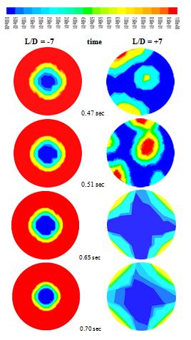
151 131

152 132

153 133

154 Figure 5-20: Colour iso-levels of water volume fraction at L/D = 7 at different times; U so = 0.6 m/s, U sw = 0.3 m/s, LES at through the pipe contraction. Red denotes water and blue denotes oil. 134

155 Figure 5-21: Colour iso-levels of water volume faction α w predicted by LES at t = 1.15 sec at different axial locations U so = 0.6 m/s, U sw = 0.3 m/s. Red denotes water and blue denotes oil 135

156 Figure 5-22: Colour iso-levels of water volume fraction α w through the pipe sudden expansion predicted by LES at t = 1.15 sec; U so = 0.6 m/s, U sw = 0.3 m/s. Red denotes water and blue denotes oil. 136

157 Figure 5-23: Colour iso-levels of water volume fraction α w through the pipe sudden expansion predicted by LES at t = 1.15 sec; U so = 0.6 m/s, U sw = 0.8 m/s. Red denotes water and blue denotes oil. 137

158 Figure 5-24: Colour iso-levels of water volume fractionα w through the pipe sudden expansion modelled by LES at t = 1.15 sec; U so = 0.6 m/s, U sw = 0.6 m/s. Red denotes water and blue denotes oil. 138

159 Figure 5-25: Colour iso-levels of water volume fraction α w through the pipe sudden expansion predicted by LES at t = 1.15 sec, U sw = 0.8 m/s, U so = 0.8 m/s. Red denotes water and blue denotes oil. 139

160 Figure 5-26: Variation of core thickness with superficial velocity, contours of water volume fraction from CFD Figure 5-27: Variation of core thickness with superficial velocity contours of water volume fraction from CFD simulations, Red denotes water and yellow denotes oil. 140

161 5.12 Summary In this work, CFD was used to model the turbulent flow of a high viscosity oil-water CAF through a contraction and an expansion in horizontal pipes. The computational mesh used for the expansion had 55,641 cells and for the contraction had 66,735 cells. The CAF simulations were performed using the VOF method in ANSYS Fluent The solver and the parameters (pressure and velocity) were set up following the values used by Das et al. [79]. The pressure velocity coupling was obtained by the PISO algorithm in ANSYS Fluent. The figures show a reasonable match in the inlet to outlet pressure drop from between the current simulation and the result presented by Das et al. [79]. The outcomes from the simulations show the ability of the VOF to predict the CAF patterns with some accuracy. The main points from this investigation are as follows: 1. LES utilizing ANSYS Fluent 16.2 was performed to predict the oil-water CAF in the contraction and expansion of 0.6 m horizontal length pipes. 2. A VOF multiphase model was selected for modelling the oil-water CAF pattern with a smooth interface. 3. Lower under relaxation factors where used when starting the CFD solver to obtain convergence. 4. The structured meshes from chapter 4 were used 5. A few predictions of the axial pressure drop distributions compared with published κ-ε results by Das et al. [79]. 6. The total pressure drop was investigated at different values of inflow surface velocities. It was determined that when the velocity increases, the total pressure drop likewise increases. 7. A separated oil layer and an oil-water wavy interface predicted by the CFD simulation, while a separated water layer was not fully predicted. This issue needs be better understood and resolved before simulating other stratified flows. 141

162 Chapter 6 CFD simulation of heavy oil water flow CAF in horizontal pipe using the LES model 6.1 Introduction This chapter aims to increase the understanding of the flow behavior of water lubricated heavy oil transport to establish risk reduction procedures in the field of heavy oil transport. Based on past investigations into water lubricated heavy oil transport, safe operational parameters for CAF have been suggested (see Anand et al. [8], Arney et al. [16], Balakhrisna et al. [18], Bannwart [20], Bannwart et al., [21], Bensakhria et al. [24], Brauner [30], Herrera et.al [66], Joseph et al., [76], Jing Shi [74], Das et al. [79] and McKibben et al. [97]). These studies have shown that, for the time being, the input water volume fraction and flow rate must be appropriate to obtain a stable CAF. However, the parameters for the safe, effective and economic operation of CAF are yet to be established. Nevertheless, in the oil industry field, it is crucial to obtain accurate predictions of heavy oil-water flow properties such as the total pressure drop, the flow regime, and effective wall friction. Many of the current models fail to account for the impact of oil fouling at the pipe wall, which can increase the total pressure drop of CAF. Simply put, CAF can be improved upon by the identification of the different flow regimes it can develop, which are determined by the inflow surface flow velocities. Moreover, CAF involves high oil densities and high oil flow rates and the heavy oil viscosity plays a main role in determining the regime flow. In addition, variations in the heavy density and pipe diameter affect the heavy oil-water flow. Previous studies mentioned in the literature review in chapter two investigate the characteristics of heavy oil and discussed how flow differs from light oil-water flow. The characteristics of heavy oil-water flow require further investigation in the contest of CAF. 6.2 Objectives The study described in this chapter was principally designed to is investigate the behavior of twophase liquid-liquid heavy oil (high viscosity)-water flow in horizontal pipes, to understand the characteristics of CAF using LES. 142

163 To fulfill the objective of this chapter, sub-aims were determined as follows: To select an LES procedure suitable for modelling CAF of heavy oil and water, which can be used with horizontal pipes of different diameters, flow rates, and velocities. To develop a CFD model for the CAF in ANSYS Fluent. To select an efficient and time-accurate incompressible FVM, to solve the filtered governing equations with SGS turbulence closure for wall-bounded annular flows through horizontal pipes. To develop a good understanding of the flow features of CAF. To develop an accurate CAF model, able to predict losses (fouling, wall friction and pressure gradient and the volume fraction of oil and water). To analyse model results and compare these with selected studies discussed in the literature review. 6.3 CFD simulation setup and model development and LES approach Introduction To date, many simulations describing two-phase liquid-liquid heavy oil-water flow have been presented by researchers utilizing the ANSYS Fluent software package. Vielma et al. [155] presented a study detailing the characterization of oil/water flows in horizontal pipes. Ghosh et al. [61] presented a simulation of core annular flow in return bends. Wang et al. [162] investigated heavy crude-water two-phase flow and its related flow characteristics. Al-Yaari et al. [7] described stratified oil-water flow in a horizontal pipe, using the VOF model. In addition, many CAF simulations used the VOF model for various pipeline geometries. For example, Ghosh et al. [60] presented a model of a downward flow, Manmatha et al. [94] described the two-phase pressure drop caused by a sudden contraction and an expansion in small circular pipes. Das et al. [79] investigated the flow through a sudden contraction and an expansion in horizontal pipes. Chen et al. [37] studied two phase flow across small sudden expansions and contractions. Anand et al. [8] described the oil-water two-phase flow characteristics in a horizontal pipeline. Yang [167] conducted a study of viscous oil and water pipe flow. Kiyoung and Haecheon [82] presented the characteristics of turbulent CAF in a vertical pipe. Roul et al. [129] studied the two phase pressure drop caused by a sudden contraction and an expansion in small circular pipes. In the CAF studies 143

164 mentioned above, geometries with co-axial inlets were used, so small diameter pipes (d = 0.012m) were assumed. In the simulation described in this chapter, a 3D CFD simulation of two-phase liquid-liquid heavy oil-water flow was conducted utilizing ANSYS Fluent with the aim of achieving greater understanding of the flow behaviours Physical model Figure 6-1 shows the computational domain used in this chapter. The domain axial length is 3 meters, and the pipe diameter is d = cm. As in chapters 4 and 5, a hexahedral mesh was created, and a third angle projection of the mesh at the inlet and outlet is provided in figure 6-2. In addition, the mesh is clustered close to the pipe wall. A mesh dependence study was conducted to determine the sensitivity of the predictions on the mesh refinement. The mesh that was finally selected comprised around cells. The physical properties of the heavy oil and water used in the simulation are listed in table 6-3. The heavy oil is in the core and water is the annular fluid. 144

165 Figure 6-1: Schematic of the flow domain and dimensions of a three dimensional CFD, and details of water and oil inlet sections. Figure 6-2: 3D unstructured grid at the inlet and outlet regions. 6.4 Numerical model This chapter uses the same numerical model as chapter 5. Specifically, it uses the method described in section 5.6. The VOF approach of section is used with the oil surface interface modelled as in section 4.4. The space filter form on the conservation laws, equations 3.18, 3.20, 3.21 and 3.22 are used with the Smagorinsky-Lilly SGS model to provide LES of the two-phase flow. 145

166 6.5 LES model ANSYS Fluent is used to solve the filtered N-S equations discretized in finite volume form. PISO and SIMPLE schemes for the LES model were utilized as in chapter 5. The Fluent second order scheme no flux limiters was used for time advancement, and linear central differencing was used to compute the diffusion terms in the LES model. The heavy oil and water superficial Reynolds numbers (Re so ) were calculated as stated in section Near-wall treatment for LES model The wall-resolved LES technique used to treat the solid wall boundaries is the same as described in section 5.8 in chapter Implementation of the numerical method Initial conditions and boundary conditions The inlet boundary, the wall boundary, and the outlet boundary are the three surfaces that bound the computational domain. The flow domain initial conditions neither affect the fully-developed turbulent flow through the pipe, nor they affect the accuracy of the results. The initial state of the computational domain should only affect the calculation time to achieve the fully developed turbulent flow stable. For any given combinations of the heavy oil and water Reynolds numbers, the corresponding water and oil surface velocities U sw and U so are obtained as shown in section 4.5 given the fluid properties in table 6-4. The flow is assumed isothermal. From the U sw and U so values and the wall no slip boundary condition, the velocity gradient order of magnitude at the wall can be estimated assuming a turbulent velocity profile. This points to a steep velocity gradient at the wall that requires a small wall-normal mesh size. With the wall-resolved LES approach of section 6.6, fine grids are required to implement this wall boundary treatment for which the computing load is likely to be very large, because of the high number of grid points. This approach is therefore limited to turbulent flows at low Reynolds numbers, and using the wall resolved boundary condition limits the development of large eddy simulations for many engineering application. 146

167 The boundary conditions for the domain are the same conditions detailed in section Boundary condition at pipe inlet Velocity Inlet In this model, the heavy oil fills the core of the horizontal pipe at the inlet, as shown in figure 6-1. Water fills the annular space of the horizontal pipe across the remainder of inlet plane. In the annular space of the water inlet at x = 0 over the range R 1 < r R 2, the velocity is axial with the profile of equation 4.29 and α w = 1. In the core space of the oil inlet at x = 0 over the range 0 r < R 1, the velocity is axial with the profile of equation 4.28 and the volume fraction of oil α o = Boundary condition at pipe outlet At the outlet, the pressure outlet boundary condition in ANSYS Fluent, with zero gauge pressure corresponding to the absolute static pressure of Pa is used. The diffusion fluxes for the variables in the exit direction are set at zero. 3. Boundary condition at pipe wall A stationary no slip boundary condition is imposed on the pipe wall, by which U = 0 The y + along the wall was estimated by equation Simulation setup The simulation was set up by using the settings recommended in the Fluent User's Guide [13]. The problem issue was solved as a transient flow using the explicit VOF model of section In this simulation, the flow is solved as turbulent whenre sw > Re sw is defined as stated in section 4.5 and its numerical values are listed in table 6-4. In this chapter, the same inner domain initialization is used as in section The same combination of schemes (PISO, SIMPLE, PRESTO!) is used as in section The same lowerorder schemes are used at the start of the computation. A time step of 10 3 s is used to maintain a stable computation by which the global Courant number is between 0.6~0.85. Convergence is monitored by on the transport equation residuals. 147

168 The convergence criterion is set at 10 6 in terms of the absolute values of the residuals for continuity, momentum equations, and turbulence equations. In addition, the static pressure and water volume fractions were monitored on different axial planes. Every simulation case in this study was kept running until the observed values had achieved statistical stationarity. Computational setup Table 6-1: Computational setup Turbulent Model LES, Smagorinsky-Lilly model Material Oil and Water Numerical details Pressure-Velocity Coupling PISO Discretization Momentum Bounded Central differencing Pressure PRESTO! Gradient Least squares cells based Time Bounded second order implicit Boundary Conditions Inlet Velocity Outlet Pressure Simulation parameters Total simulation time sec Start data sampling 40 sec Time step sec Courant number 0.5 to 0.85 in all simulations Residual Criteria 1E

169 ANSYS Fluent solution controls Table 6-2: ANSYS Fluent solution control method Momentum Explicit Relaxation Factor 0.3 Pressure Explicit Relaxation Factor 0.3 The Under-Relaxation Factors for density and body forces were retained at their default value of Simulations The geometry detailed in figure 6-2 was used to run the simulations in this chapter. Which used the numerical models and solution setup parameters presented in sections For validation purposes, the simulations were performed at the flow conditions described by Charles et al. [36]. The validated model was then used to explore a wider envelope of flow conditions. Table 6-3 presents the flow conditions used in the simulations in this chapter. 6.8 Results and discussion The CFD results in this chapter were analyzed to determine the lows regimes, the volume fraction discretization of the water-lubricated flow, and the axial pressure gradient. The CFD results conducted in this chapter were also validated by comparison with those described by Charles et al. [36]. To gain some insight in the flow regime, cross-sectional flow features and their associated characteristics are investigated. The effects of the mesh size, the initialization method, the turbulence model, and the water-oil interface reconstruction scheme were studied. Table 6-3: Fluid Properties Notation Low viscosity LV-1 Low Viscosity LV-1-2 Low Viscosity LV-2 Water density (ρ), kg/m 3 Water viscosity (μ), Pa.s Oil density (ρ), kg/m 3 Oil viscosity (μ), Pa.s Water velocity (U sw ) m/s Oil velocity (U so ) m/s Reynolds number of water (Re sw ) Reynolds number of oil (Re so ) Source Charles et al. [36] Charles et al. [36] Charles et al. [36] 149

170 Charles LV-3 et al. [36] Charles LV et al. [36] Charles LV-3-3 et al. [36] Charles LV-3-4 et al. [36] HV Present study HV-1-2 HV Present study Present study HV Present study HV Present study HV-4 HV-4-2 HV-4-3 HV-4-4 HV-5 HV-6 HV-7 HV Present study Present study Present study Present study Present study Present study Present study Present study 150

171 6.8.1 Effect of the domain initialization method To study and investigate the impact of the initialization method on the flow field, HV-3 and HV- 3-2 simulations, as mentioned in table 6-3 were performed. In HV-3, the flow field was initialized according to the set water inlet boundary conditions, while in simulation HV-3-2 it was initialized relative to the oil inlet boundary conditions. Figure 6-3 outlines the evolution over time of the oil volume fraction. Although a match in the volume fraction between the two test cases is not achieved at t = 0.95 sec, both the predictions show a common tendency to develop a core oil flow. The water initialization technique is utilized as for the remainder of this chapter. (a) Domain initialization from the oil inflow (b) Domain initialization from the water inflow Figure 6-3: Development of core flow with simulation time. (a) Domain initialization from the water inflow (HV-3); (b) Domain initialization from the oil inflow (HV-3-2). Colour iso-levels of the oil volume fraction from LES. Red denotes oil and blue denotes water. 151

172 6.8.2 Effect of the oil-water interface reconstruction method The oil-water interface reconstruction method affects the predicted shape of the interface. The Geo-Reconstruct scheme is described in section 4.6 recommended for general use by ANSYS Fluent. As indicated by the Fluent Theory User Guide [13], the CICSAM (Compressive Interface Capturing Scheme for Arbitrary Meshes) scheme is more appropriate for flows with a viscosity ratio between the phases, where the CICSAM scheme is responsible for selecting the finite difference scheme. Therefore, two simulations, HV-1 and HV-1-2, were performed to determine which phase interface reconstruction scheme is better for the current application. Figure 6-4 shows the oi volume fraction obtained by the Geo-Reconstruct scheme and by the CICSAM scheme. Both methods predict a CAF. Nevertheless, the interface shape between the heavy oil and the water differs substantially. The interface predicted by the CICSAM scheme is very smooth, without any noticeable waviness. Interface waviness is produced by the Geo-Reconstruction scheme. This waviness is also present in experiments at similar flow conditions, Charles et al. [36]. Therefore, the Geo-Reconstruct scheme is used for the remainder of this chapter. 152

173 Volume fraction (oil) (a) Meridional plane and L/D = +10 Volume fraction (oil) (b) Meridional plane and L/D = +10 Figure 6-4: Colour iso-levels of the oil volume fraction predicted by LES with (a) The CICSAM scheme (HV-1-2) and (b) The Geo-Reconstruction (HV-1). Red denotes oil and blue denotes water Effect the sub-grid-scale model The Smagorinsky-Lilly, WALE, WMLES and WMLES S-Omega models are the sub-grid-scale models available in ANSYS Fluent for two-phase flow simulations. These four models were tested to determine which one is the most appropriate for a two-phase (oil-water) flow simulation. Figure 6-5 presents the predictions from applying various SGS models and the corresponding experiments, Charles et al. [36]. It is shown that all SGS models produce CAF. Among these, the WMALES S-Omega model provides the first prediction of the pressure gradient. The experimental flow pattern is taken from Charles et al. [36]. Essentially, it is not specified in Charles et al. [36] the flow visualization has some level of deformation. Figure 6-6 illustrates the distribution of the turbulence variables at the same axial plane L/D = +10 obtained by different SGS models. The turbulence properties computed from the Smagorinsky-Lilly and the WALE models were found to be similar. The magnitudes of the turbulence properties computed using the WMLES S-Omega 153

174 model are smaller than those predicted by the Smagorinsky-Lilly and WALE models, but they are still of the same order of magnitude. Figure 6-5: Colour iso-levels of oil mass fraction predicted by LES at t = Sec with different SGS models and comparison with experimental flow visualization by Charles et al. [36]. In the experiment, black illustrates water and white with dots inside illustrates oil. In LES, red denotes oil and blue denotes water. The pressure gradient from different SGS models versus the experiment, with percentage differences. 154

175 155

176 156

177 157

178 Figure 6-6: Axial plane distribution of turbulent quantities predicted by different SGS models at L/D = +10 and t = sec. (a) Smagorinsky-Lilly model (LV-3-2); (b) WALE model (LV-3-3); (c) WMLES (LV-3-4); (d) WMLES S-Omega model (LV-3) 158

179 6.8.4 Comparison simulation results with experimental flow study The simulations LV-1, LV-2 and LV-3 were performed at the same flow conditions as the experiment by Charles et al. [36]. The experiment by Charles et al. [36] used low-viscosity oil ( Pa.s) water to develop a CAF. The simulations and experiment are compared in figure 6-7. There is a qualitative agreement in the flow pattern between the two sets of flow visualization. The oil-water surface interface is essentially non-wavy and located close to the pipe wall in LV-1 in both experiment and computation. Evidence of more wavy interface is given in both experiment and computation for LV-3. Figure 6-8 uses the same LES methods in figure 6-7 to predict CAF for heavy oil and water with five different surface velocities combinations for heavy oil and water. All configurations show the basic CAF of a core heavy oil flow surrounded by an annulus of water. As the surface velocities increase, the water annulus thickness appears to reduce until the oil-water interface touches the pipe walls in HV-8. This causes oil fouling. To attain a clears view of how heavy oil fouling evolves over time at the pipe wall, the oil volume fraction is shown across 4 axial planes at four progressive times. Limited linked between the heavy oil core and the pipe wall and heavy oil fouling spots can be seen in the computed volume fraction of figures 6-9 (c) and (d). L-1 L-3 Figure 6-7: Comparison of predicted CAF by LES and the Smagorinsky-Lilly SGS at t = sec with the experiment from Charles et al. [36]. In Charles et al. [36], the black denotes water and the white with dots inside denotes oil. Colour iso-levels of oil volume fraction from CFD, the red denotes oil and the blue denotes water. 159

180 Figure 6-8: Comparison of predicted CAF by LES with the Smagorinsky- Lilly SGS model at t = sec with five different superficial oil and water velocity combinations. Colours iso-levels of oil volume fraction. Red denotes oil and blue denotes water 160

181 Figure 6-9: Colour iso-levels of oil volume fraction across four axial planes predicted for cases (a) HV-2 and t = sec, (b) HV-7 and t = sec, (c) HV-7 and t = sec and HV- 8 and t = sec. Red denotes oil and blue denotes water. 161

182 6.8.5 Cross-sectional flow characteristics of CAF Figure presents the oil volume fraction and the axial velocity profiles at various axial positions on the meridional plane, for low viscosity CAF. Figure 6.-10a indicates a laminar flow state and a typical CAF with the inflow volume fraction not evolving node with axial distance. Figures 6-10b and 6-10c indicate a turbulent flow state, as the profile of the oil volume fraction differs according to the axial location, reflecting the waviness of the phase interface in the flow. Differing from the velocity profile that would be expected in a single-phase flow, the velocity profile along the pipe varies according to the flow state, because of the change in the phase interface surface. The velocity profile at x = 0 in figure 6.10a indicates a region of lower velocity close to the upper wall with respect to the other profiles. This is not physically possible as the profile meant to be fully developed. This is therefore probably a numerical effect of the imposed inflow boundary conditions. The velocity profiles of figures 6.10b and 6.10c show an increment in bulk velocity with increasing axial distance. This behavior cannot simply be explained by the change in position of the phase interface surface and looks more like a pipe entry length effect, although there is insufficient growth of wall boundary layer thickness. The whole flow appears to be accelerating towards the outlet. This may indicate an insufficient total simulation time for achieving a statistically stationary flow. Figures 6-10b and 6-10c show the velocity profile resulting from the annular flow, which is akin to that from a turbulent single-phase flow. At the water-oil phase interface, the velocity gradient has no sharp change. The simulation indicates that the maximum velocity changes from 1.15 m/s to 1.35 m/s with a change in the Reynolds number Re sw from 6,331 to 14,271. Figure 6.11 shows radial profiles of the sub-grid-scale eddy viscosity μ t from equation 3.32 on the meridional plane at different axial positions. CAF for low-viscosity oil is modelled in figure The sub-grid-scale eddy viscosity μ t illustrates the turbulence strength. Figure 6-11 indicates the distribution of sub-grid-scale viscosity is physically sound. Specifically, it is shown that the turbulence intensity is low in the central section of pipe, where the oil core flows. The oil viscosity 162

183 used in these simulations is kg/m-s and at this value of viscosity the oil flow phase is laminar. With reference to the location of the oil-water interface surface shown in figures 6-10b and 6-10c. Figures 6-11(b) and 6-11(c) show that the turbulent intensity is low at the pipe wall and at the oilwater interface surface, because of the oil phase viscosity and of the no-slip wall. While the maximum sub-grid-scale eddy viscosity is located in the annular water layer close to the pipe wall. Comparing figures 6-11a and 6-11b shows that the turbulence intensity in the annular water layer increases as the water flow rate rises. Figure 6-12 shows the LES predictions of the oil volume fraction phase of axial velocity profiles and velocity by radial profiles at different axial locations for heavy oil CAF. Figures 6-12a, 6-12b and 6-12c show the effect of increasing the water density from HV-4 to HV-5 and of increasing the inflow momentums from HV-4 to HV-8 Compared figure 6-10, the velocity profiles of heavy oil core are flatter, due to the heavy oil viscosity being 0.22 kg/m-s, almost 200 times that of the water. These simulations show that, when the oil viscosity is significantly higher than water viscosity, the oil is essentially flowing inside the water as a solid body. This is a hypothesis that has been applied by Ooms et al. [108] and Zhang et al. [171] and is validated by the current LES results. This hypothesis only holds if the oil viscosity is substantially higher than the water viscosity as in HV-4, HV-5 and HV-8. Figure 6-10 shows that the oil core cannot be modelled as a solid body when the heavy oil viscosity is only one order of magnitude higher than the water viscosity. The comparison among figures 6-12a, 6-12b, and 6-12c, shows that the velocity distribution for CAF varies in relation to the flow state. Figures 6-12b and 6-12c show developed CAF, where the velocity profile is almost symmetric. In HV-4, HV-5vand HV-6, the oil core almost flows as a rigid body, with a higher axial total velocity than the annular water layer. The velocity reduces rapidly towards the pipe wall in the annular water layer. Figure 6-12a indicates a CAF in which the upper water layer is extremely thin and the base water layer is comparatively thicker. As a consequence, the velocity distribution for CAF is symmetric. 163

184 Figures 6-12b and 6-12c show that the oil-water slip ratios as determined by the phase velocity ratios, U o /U w, averaged across the pipe cross-section, are higher than 1 for the HV-5 and HV-6 cases, while figure 6-12a reveals that the oil-water slip ratios is a slightly less than 1 for the HV-4 case. Figures 6-12b and 6-12c show the relative water layer heights for the two simulations of CAF, which are nearly similar, at around 10% to 20% of the pipe width. The absolute thickness of the water layer is instead much higher for the case shown in figure 6-12a. Figure 6-12c shows that the oil volume fraction profile for HV-8 reaches the value of 1.0 over a smaller distance away from the walls than the equivalent profiles in figures 6-12a and 6-12b. At move of the four axial locations the volume fraction at the wall differs from zero and this indicates that at these axial positions and at this computational time no oil fouling is predicted Figure 6-13 shows the radial profiles of the sub-grid-scale eddy viscosity μ t of heavy oil-water CAF at the same axial positions as in figure The radial distribution of the sub-grid-scale eddy viscosity correlated with oil volume fraction distribution by which higher values of μ t are predicted in the annular water layer, lower values of μ t are predicted across the high-viscosity oil core. Comparing figures 6-13 and 6-11 shows, that the sub-grid-scale eddy viscosity in the oil core for high viscosity oil CAF is lower than that for low-viscosity oil CAF. In fact, in figure 6-13, the subgrid-scale eddy viscosity for the oil core is around 10.8 to m 2 /s 1, while in figure 6-11 the sub-grid-scale eddy viscosity is 10.5 m 2 s 1. If the oil viscosity is high, then, a less turbulent flow can be obtained. 164

185 (1) (2) (a) Simulation at LV-1 165

186 (1) (2) (b) Simulation at LV-2 166

187 (1) (2) (c) Simulation at LV-3 Figure 6-10: Oil phase volume fraction and axial velocity profiles of low viscosity CAF at various axial positions. Predictions by LES with the Smagorinsky-Lilly model at t = 10.2 seconds 167

188 (1) (2) (a) Simulation at LV-1 168

189 m 2 s 1 (1) m 2 s 1 (2) (b) Simulation at LV-2 169

190 m 2 s 1 (1) (2) (c) Simulation at LV-3 Figure 6-11: Sub-grid-scale eddy viscosity μ t and effective eddy viscosity of low-viscosity CAF at various axial. Predictions by LES with SGS model by the Smagorinsky-Lilly model at time t = 10.2 seconds 170

191 (1) (2) (a) Simulation at HV-4 171

192 (1) (2) (b) Simulation at HV-5 172

193 (1) (2) (c) Simulation at HV-8 Figure 6-12: Oil phase volume fraction and axial velocity profiles of high viscosity oil and water CAF at various axial positions. Predictions by LES with the SGS model by the Smagorinsky-Lilly at t = seconds 173

194 (1) (2) (a) Simulation at HV-4 174

195 (1) (2) (b) Simulation at HV-5 175

196 m 2 s 1 (1) (2) (c) Simulation at HV-8 Figure 6-13: Sub-grid-scale eddy viscosity μ t and effective eddy viscosity of high-viscosity CAF at various axial positions. Predictions by LES with the SGS model by the Smagorinsky-Lilly at t = seconds 176

197 6.9 Summary This chapter described, adopted and utilized the VOF model in association with Smagorinsky- Lilly model to simulate CAF. The flow parameters and the simulation setup were described. The simulation was set up based on results from preliminary simulations. Investigations concerning the effects of the mesh size, initialization method of the water-oil interface geometric reconstruction, and of the sub-grid-scale model were conducted and can be summarized as follows: Numerical errors occurred because of the spatial discretization and a mesh was chosen from the mesh dependence study. The oil initialization method and the water initialization method provided simulation results compatible with experiments presented by Charles et al. [36]. As a result, the water initialization method was chosen to save computational time. The Geo-Reconstruct scheme was chosen to reconstruct the phase interface surface between oil and water The CFD results illustrate aspects of the flow regime, pressure gradients, and cross-sectional flow characteristics. The LES were compared against experimental results provided by Charles et al. [36] for validation purposes. From the simulation of the low-viscosity oil-water flow, a reasonable agreement is shown between the simulation and the experiment. For high viscosity oil-water flow, an oil fouling film on the pipe wall was not captured for most of the simulation situations. This is a fundamental issue that points to an inadequate physical representation of wall adhesion as implemented in Fluent. The variation of CAF between the velocity profiles for light oil-water and heavy oil-water combinations was indicated. With a turbulent water flow, the velocity distribution for CAF with a light oil is broadly like that of a turbulent single-phase flow. The velocity distribution of CAF with a heavy oil is characterized by almost steady velocity towards the heavy oil. It can be assume that the heavy oil flows inside the annular water layer film as a rigid body if the oil viscosity is extremely higher than the water viscosity. The turbulence intensity distribution correlates with the oil volume fraction distribution, with high turbulence intensity in the water and low turbulence intensity in the heavy oil. 177

198 Chapter 7 CFD simulation of heavy oil-water-air flow through a horizontal pipe using an LES model 7.1 Objectives The main objective of the study reported in this chapter is to investigate the CAF of heavy oil, water and air flow numerically under various conditions of temperature and volume fractions of air. 7.2 Numerical formulation and methodology LES are well suited for performing small-scale simulations that produce flow predictions resolved in space and in time. Consequently, the LES approach has been utilized through a horizontal pipe in the study described in this chapter. The model results were validated against reference predictions reported by Ferreira et al. [14]. 7.3 CFD Simulation of LES for CAF in the horizontal pipe Three-phase flow in a horizontal pipe in a 3D model was generated as indicated in figure 7-1. It should be emphasized that heavy crude oil, water, and air were all utilized as inlet fluids. The pipe was modelled. The model used in this chapter is the same as the one used in chapter 6. The hexahedral structured mesh utilized for the present work is the same as the one used in section in chapter

199 Figure 7-1: Schematic of the flow domain and dimensions of a three dimensional CFD, and details of water and oil-air inlet sections. Table 7-1: Thermo-physical properties of the three fluid phases (25 C) used in the present study Property Water Phase Oil Phase Air Phase Density (ρ), kg/m Viscosity (μ), Pa.s e 05 Specific heat (J/kg K) 4181, , ,766 Interfacial Tension N/m at 25 Celsius

200 Table 7-2: Horizontal pipe geometry dimensions Horizontal pipe Length Diameter 3 m 2.84 cm The viscosity of the three phases (heavy crude oil, water and air) for the CAF model flow in the horizontal pipe was calculated using the equations in table 7.3, derived from different sources. The equations used to obtain the viscosity of heavy oil, water, and air were given by Kreith and Bohn [83], Santana et al. [137], and Trevisan [146]. Table 7-3: Equations of the three fluid phases used to estimate the viscosity Phases Equations Units Heavy oil μ o = e ( T) Pa-s Water μ w = ( T Air μ g = T Pa-s where T is the temperature of the fluid in Celsius The viscosity equation relies on data provided by Kreith and Bohn [83]. The temperature range was 0 C T 100 C. Pa-s 7.4 VOF model The VOF model of section is used to simulate the three phase flow. The accuracy of the VOF model falls when the interface length scales approach the computational grid scale. Therefore, the VOF model can be considered appropriate for multiphase flows where the interface length scale is large. The interface between the heavy oil and the water has a characteristic length larger than the pipe diameter; therefore, the VOF model can be considered an appropriate model for the modelling of CAF in a pipeline. 180

201 7.5 Model development and LES approach Physical model In this chapter, the oil-water-air model by Ferreira et al. [14] is reproduced and the computational domain of section 6.3.2, figure 6-1, and the numerical mesh of figure 6-2 were used. The oil inlet in figure 6-1 was used as the oil-air mixture inlet with some simplifications and modifications. A 3D two-phase of heavy oil, water and air for the CAF through a horizontal pipe was created as shown in figure 7-1. The air phase was not modelled by a VOF approach but it was combined with the oil phase as an oil-air mixture. Heavy oil forms the core (viscosity µ = 0.64 Pa-s and density ρ = 971 kg/m 3 ), and water is the annular fluid (viscosity µ = Pa-s and density ρ = kg/m 3 ) Governing equations This chapter uses an extension of the numerical model of chapter 5. The extension allows the removal of the assumption of an isothermal flow. The VOF approach of section is used with the water-oil interface surface modelled as in section 4.4. The space-filtered version of the conservation of volume fraction and of the momentum of equations and 3.22 are used with the SGS model of Smagorinsky-Lilly, to provide an LES of the two-phase flow. As the flow is no longer assumed isothermal, the conservation of energy equation 3.5 is used to determine the temperature distribution. The specific is assumed to be constant and the relationship between energy e and temperature T is e = c p T. Therefore, the energy equation can be stated as: T t + U. T = v Pr. T (7.1) where the Prandtl number is defined as Pr = c pv, and k is the thermal conductivity. ρk C p, v, ρ and k are mixture properties estimated according to the water, oil and air volume fractions (α w, α o, α a ) as C p = C po α o + C pw α w + C pa α a and by similar expressions for v, ρ and k. By applying the same space filtering technique of section 3.5, the energy equation becomes: 181

202 T + U. T =. ( v + v t ) T (7.2) t Pr Pr t where a bar denotes a quantity that has been spatially filtered, and v t is the SGS kinematic eddy viscosity, which is evaluated as in section 3.5.1, equation Numerical methodology The PISO scheme for the LES model was utilized in this chapter. A second order scheme was used without flux limiters for time advancement and linear central differentiation was used to compute the diffusion terms. The heavy oil and water superficial Reynolds numbers (Reso) were calculated as stated in section 4.5. The air superficial Reynolds number is Re sa = DU saρ a μ a where subscript a denotes the air phase and the subscript s denotes the superficial conditions. D, ρ, μ and U denote the inlet pipe s diameter, density, viscosity, and velocity respectively. 7.7 Boundary conditions 4. Boundary condition at pipe inlet Velocity Inlet In this model, a heavy oil and air mixture forms a core through the horizontal pipe inlet. The water fills the horizontal pipes annular space inlet. This is shown in figure 7.1. The annular water inflow is imposed as stated in section with a uniform temperature T w, for R 1 < r < R 2. In the core space representing the oil-air mixture inlet, 0 r < R 1, the mixture velocity is defined as axial the profile defined by equation In this chapter, U o of equation 4.28 refers to the oilwater mixture bulk velocity. The volume fraction of oil and air are α o = 0.95, α a = 0.05 and the temperature T = T o = T a is uniform. The fluid is allowed to flow from the inlet at a bulk velocity of the oil-air mixture of 1.5 m/s and water of 2.2 m/s. (7.3) 182

203 5. Boundary condition at pipe outlet At the outlet, a pressure outlet is used and the diffusion fluxes are set to zero. At the outlet section (x = L), a constant mean absolute pressure pest = 101,325 Pa, was specified, where L is the pipe length. 6. Boundary conditions at pipe wall A stationary no slip boundary condition was imposed on the pipe wall. The wall was assumed isothermal at T p =288K. In this chapter, a root mean square (RMS) residue equal to 10 7 kg/s was set as the convergence standard. The properties of the liquids utilized in the simulation are given in tables 7-1, 7-2 and Interface treatment and near-wall treatment of the LES model In this chapter, the interface surface between the oil-air mixture and water was treated by using the same techniques in section 6.6. As well the technique used to treat the solid wall boundaries is the same as the one in section Computational set-up and numerical procedure In this chapter, the numerical method that is used for solving the discrete governing equations is same as the one used in section The solver options used in ANSYS Fluent are listed in Table 7-5. Numerical values for the inlet velocities, density and viscosity were set, based on a study by Ferreira et al. [14], as shown in Tables 7-1 and 7-2. In addition, the velocity inlet profile was imposed as in section

204 ANSYS Fluent solution controls Table 7-4: ANSYS Fluent solution control method Momentum Explicit Relaxation Factor 0.3 Pressure Explicit Relaxation Factor 0.3 The Under-Relaxation Factors for density and body forces retained at a default value of 0.8 Computational setup Table 7-5: Computational setup Turbulent Model LES, Smagorinsky-Lilly model Material Oil, Water and air Numerical details Pressure-Velocity Coupling PISO Discretization Momentum Bounded Central differencing Pressure PRESTO! Gradient Least square cells based Time Bounded second order implicit Boundary Conditions Inlet Velocity Outlet Pressure Simulation parameters Total simulation time sec Start data sampling 40 sec Time step sec Courant number 0.5 to 0.85 in all simulations Residual Criteria 1E

205 Y (m) Results and discussion Impact of the air phase The radial profiles of superficial velocity for oil and water are shown in the figures 7-2, 7-3, 7-4, and 7-5, for the oil-water simulation and for the oil-water-air simulation at four axial locations X = 0 mm X = 1000 mm X = 2000 mm X = 3000 mm u so m/s Figure 7-2: Radial profiles of superficial velocity for oil in the heavy oil-water flow at various axial positions. LES at t = seconds 185

206 Y (m) Figure 7-3: Radial profiles of superficial velocity for oil in the heavy oil-water flow at various axial positions. LES at t = seconds 186

207 Y (m) Figure 7-4: Radial profiles of superficial velocity for oil in the heavy oil-water flow at various axial positions. LES at t = 14.3 seconds. T = K Based on the velocity profiles shown in figures 7-.2, , and 7-5, it cannot be asserted that when the air phase is introduced to heavy oil-water flow, this causes important changes in the fluid dynamics of the water and oil phases. In theory, the air phase should affect the velocity gradient in the lower area of the pipe, because of rising in water flow in that area. This behaviour was independently observed by Bannwart et al. [19], Poesio et al. [113], Poesio et al. [117] and Strazza et al. [143]. 187

208 Y (m) Y (m) X = 0 mm X = 1000 mm X = 2000 mm X = 3000 mm Figure 7-5: Radial profiles of superficial velocity for oil in the heavy oil-water flow at various axial positions. LES at t = 14.7 seconds. T = K Figure 7-6: Radial profiles of superficial velocity for oil in the heavy oil-water flow at various axial positions. LES at t = 14.1 seconds. T = K 188

209 Y (m) Figure 7-7: Radial profiles of superficial velocity for oil in the heavy oil-water flow at various axial positions. LES at t = seconds. T = K Figure 7-8: Colour iso-levels of oil volume fraction at T = K in heavy oil water air LES at various axial planes. LES at t = 14.3 seconds. Red denotes oil and blue denotes water. 189

210 Figure 7-9: Colour iso-levels of oil volume fraction at T = K in heavy oil water air LES at various axial planes. LES at t = 14.7 seconds. Red denotes oil and blue denotes water. Figure 7-10: Colour iso-levels of oil volume fraction at T = K in heavy oil water air LES at various axial planes. LES at t = 14.1 seconds. Red denotes oil and blue denotes water. 190

211 Figure 7-11: Colour iso-levels of oil volume fraction at T = K in heavy oil water air LES at various axial planes. LES at t = seconds. Red denotes oil and blue denotes water Impact of temperature change Superficial velocity profiles for the heavy oil-water-air flow at various temperatures ( K, K and K) when measured on the axial positions equal to X = 1000 mm and Z = 0 mm are illustrated in figure It is observed that a rise in the temperature of the phases through the pipe inlet results in a small difference in the oil phase superficial velocity, due to a change in the viscosity. 191

212 Y (m) Figure 7-12: Predicted radial profiles of oil superficial velocity at various temperatures at X = 1000 mm and Z = 0. LES at t = 14.7 seconds. Oil-air-water simulation. The axial plane volume fraction distribution for the oil phase at X = 1000 mm, for various temperatures ( K, K, K and K) of the three phases at the pipe entrance, as shown in figure It is predicted that as the temperature rises, the oil also rises towards the top of the pipe. The impact of temperature changes results in a decrease in oil viscosity and hence the impedance to the flow of this fluid, created by viscous forces, is also decreased. 192

213 Figure 7-13: Colour iso-levels of predicted oil volume fraction for various temperatures, on an axial plane at 1000 mm from the entrance. LES of oil-water-air flow at t = 14.7 seconds. Red denotes oil and blue denotes water Impact of temperature and of the presence of air on the pressure drop Table 7-7 listed the predicted values for the pressure drop as a function of temperature for twophase flow ( K for T w and T o only) and heavy oil water air flow ( K, K, K and K for T 0, T w and T a ). It appears that for heavy oil-water-air, an increase in temperature reduces pressure drop, P. This arises because of the reduction in viscosity of oil and water as temperature rises from equation mentioned in table 7-3, which reduces the resistance to flow in the pipe, causing a decrease in the pressure drop. Due to the increased temperature, the viscosity of the air also rises, but as air occupies a small volume fraction, thus, the influence is small relative to that in the heavy oil and water. When heavy oil-water flow ( K for T w and T o only) is compared with heavy oil-water-air ( K for T 0, T w and T a ), the existence of air is shown to cause rise in the pressure drop of the flow. Bannwart et al. [19] and Trevisan [146] have presented and explained that a similar behaviour affects the simultaneous flow of heavy oil, water, and air. Simply put, these results were obtained because the presence of air increases the velocity of the fluid. In addition, the rise in velocity further rise the friction factor, thus increasing the pressure drop in the heavy oil water flow. 193

214 Table 7-6: Pressure drop as a function of the temperature of the mixture at the inlet of the pipe Cases T o, T w and T a (K) P (Pa/m) (Two-Phase) (T o and T w ) (Three-Phase) (Three-Phase) (Three-Phase) (Three-Phase) Temperature profiles fields The temperature profiles ( K) for oil and water at (0 m, 1 m, 2 m and 3 m) axial positions along the pipe are shown in figures 7-14 and The water temperature at the pipe inlet (0 m) is uniform, because this is the imposed inflow boundary conditions. As the flow moves away from the pipe inlet area, the temperature starts to fall. Near the pipe wall, an active, strong temperature gradient can be noticed, because of the isothermal wall boundary condition. The oil temperature profile along the pipe, as shown in figure 7-14, is almost uniform in the central region of the pipe. However, as the oil starts to move further away from the entrance to the pipe, a small temperature reduction can be observed. This can be attributed to heat transfer, because the temperature of the pipe wall is lower than the oil temperature. The radial profiles of water temperature at different axial positions are given in figure These show that water experiences the greatest reduction in temperature in the upper area of the pipe. This is because of the tendency water has to aggregate in the lower area, therefore the film of water located above the oil flow is moderately thinner. This film accordingly is more affected by the low temperature given to the pipe wall. By comparing figure 7-14 and figure 7-15 it emerges that the temperature of the oil is greater than the temperature of the water at the pipe exit. This is because the water flows near to the pipe wall, preventing the direct linked between the heavy oil and the pipe wall. Accordingly, the water acts as a thermal insulator. 194

215 Y (m) In addition, figures 7-16, 7-17, and 7-18 display the radial profiles for inlet flow temperatures of oil temperature K, K and K at four different axial positions showing that there are uniform temperature cross-sections in the central region of the pipe too. However, as the oil starts to moves further away from the entrance to the pipe, a small temperature reduction can be observed X = 0 mm X = 1000 mm X = 2000 mm X = 3000 mm T (K) Figure 7-14: Radial profiles of heavy oil temperature at four axial positions (X) along the pipe, at Z = 0 m and T = K 195

216 Y (m) Y (m) X = 0 mm X = 1000 mm X = 2000 mm X = 3000 mm T (K) Figure 7-15: Radial profiles of water temperature at four axial positions (X) along the pipe, at Z = 0 m and T = K X = 0 mm X = 1000 mm X = 2000 mm X = 3000 mm T (K) Figure 7-16: Radial profiles of heavy oil temperature at four axial positions (X) along the pipe, at Z = 0 m and T = K 196

217 Y (m) Y (m) X = 0 mm X = 1000 mm X = 2000 mm X = 3000 mm T (K) Figure 7-17: Radial profiles of heavy oil temperature at four axial positions (X) along the pipe, at Z = 0 m and T = K X = 0 mm X = 1000 mm X = 2000 mm X = 3000 mm T (K) Figure 7-18: Radial profiles of heavy oil temperature at four axial positions (X) along the pipe, at Z = 0 m and T = K 197

218 The axial plane distribution of temperature for oil and water for an inflow temperature of K is shown at X = 1000 mm in figures 7-19, and Figures 7-21 and describe the axial plane distribution of the oil temperature for inflow temperatures of K and K respectively, at X = 1000 mm. The discharges shown in Figures 7-15 and 7-16 illustrate the distributions of the temperature in oil and water phases vary through the pipe, where the water is subjected to the greater fluctuation and a higher reduction in temperature. Oil temperature (K) Figure 7-19: Oil temperature field ( K) in the YZ plane at X = 1000 mm, along the horizontal pipe 198

219 Water temperature (K) Figure 7-20: Water temperature ( K) field in the XY plane along the horizontal pipe 199

220 Oil temperature (K) Figure 7-21: Oil temperature field ( K) in the YZ plane at X = 1000 mm, along the horizontal pipe Oil temperature (K) Figure 7-22: Oil temperature field ( K) in the YZ plane at X = 1000 mm, along the horizontal pipe 200