ABSTRACT. Title of Document: PERFORMANCE MODELING OF A H 2 - FUELED PROTON EXCHANGE MEMBRANE FUEL CELL

Transcription

1 ABSTRACT Title of Document: PERFORMANCE MODELING OF A H 2 - FUELED PROTON EXCHANGE MEMBRANE FUEL CELL Eric Bennet Shields, Master of Science, 2007 Directed By: Associate Professor, Dr. Gregory Jackson, Mechanical Engineering To assist in the development of an integrated proton exchange membrane fuel cell (PEMFC) system, a 2-D fuel cell model has been developed and integrated with supporting zero-d models. The fuel cell model employs a finite-volume discretization of the conservation equations in the gas-phase flow channels, for the gas diffusion layer, and at the electrocatalyst electrolyte interface. The resulting conservation equations are converted into a DAE form for transient integration within MATLAB. The model employs detailed surface thermochemistry within CANTERA for the catalyst and electrolyte surfaces. In this study, the model was used to investigate the isothermal performance of the fuel cell and to assess how steady-state overpotentials depend on operating conditions. These results were validated against existing data supplied by Ballard Power Systems. After validation, the Ballard stack parameters were used in transient integration to evaluate how the fuel cell responds to rapid changes in load and flow conditions.

2 MODELING STEADY STATE AND TRANSIENT PERFORMANCE OF A PROTON EXCHANGE MEMBRANE FUEL CELL SYSTEM By Eric Bennet Shields Thesis submitted to the Faculty of the Graduate School of the University of Maryland, College Park, in partial fulfillment of the requirements for the degree of Master of Science 2007 Advisory Committee: Professor Gregory Jackson, Chair Professor Reinhard Radermacher Professor Elias Balaras

3 Copyright by Eric Bennet Shields 2007

4 Acknowledgements Because of the collaborative nature of this research, there have been many contributions by other members of my research group which cannot go without mentioning. Early work by Steven DeCaluwe, and talks I have had with him over the past two years, have been helpful in the development of this model. Since his work with solidoxide fuel cell modeling had many of the same goals as my own work, his advice and suggestions were insightful. The system level architecture, originally outlined and written by Professor Gregory Jackson, was developed and improved upon by Atul Bhargav and myself. In addition, his work with palladium membrane modeling dealt with many of the same issues as this fuel cell model, and discussions with him were most helpful near the completion of the code. Talks with Joshua Pearlman were helpful based on his knowledge of the fuel cell system spreadsheet calculator developed by our research group, and also from his practical knowledge of real world balance of plant components and systems. Dr. Seyed Reihani, contributed valuable experience and knowledge to my work through the many meetings I have had with him through the past two years. His ii

5 expertise with such models provided insight into many of the issues that I struggled with throughout the development phase. Mr. Patrick Hearn was instrumental in providing realistic operational knowledge to the model, and talks with him helped to ground the model in reality. His guidance, and access to experimental data, contributed to the model s eventual success. Finally, my advisor Dr. Gregory Jackson gave continual guidance and support during the development of this code, even during his sabbatical in Switzerland. His guidance led to a development tool which may be used for a wide range of studies in future work by this research group. I would also like to acknowledge the Army Research Lab for funding this research in conjunction with Ballard Power Systems Vancouver, BC. iii

6 Table of Contents Acknowledgements...ii Table of Contents...iv List of Figures...vi Nomenclature... viii Chapter 1: Introduction Introduction to PEM Fuel Cell Portable Generators Overview of PEM Fuel Cell Membrane Electrode Assembly Overview of PEM Fuel Cell Stack Overview of PEM Fuel Cell System Modeling PEM Fuel Cells PEM Fuel Cell MEA modeling PEM Fuel Cell Stack Modeling PEM Fuel Cell System Modeling Context and Objectives of Current Research...19 Chapter 2: Model Development Introduction to Model Development MEA Model Development TPB Modeling Electrolyte Modeling Gas Diffusion Layer Modeling Channel Flow Modeling Heat Transfer and Coolant Flow Modeling Fuel Cell System Modeling Low Pressure Compressor Gas-to-Gas Humidifier Numerical Techniques Model Testing and Validation...60 Chapter 3: Steady State Simulations Simulation Objectives Model Predictions at Baseline Conditions Model Predictions of Performance Voltage-Current Relationships Effects of Operating Pressures Temperature Effects Effects of Stoichiometric Ratio Sensitivity Analysis...83 Chapter 4: Transient Simulations Introduction Stack Response to Ramps in Load Stepped Voltage Constant Load Flow Rate Ramp...99 Chapter 5: Conclusion iv

7 5.1 Summary of Results Steady State Results Summary of Transient Results Recommendations for Future Work Bibliography v

8 List of Figures Figure 1 Fuel cell channel diagram...3 Figure 2 Fuel PEM fuel cell diagram...5 Figure 3 Vertical voltage distribution through the depth of a PEM MEA operating at 0.5 A/cm Figure 4 PEMFC stack diagram...10 Figure 5 PEMFC system level diagram incorporating fuel reforming and H2 separation for providing fuel flow and a compressor and GTG humidifier for providing cathode flow (adapted from (Bhargav 2006))...13 Figure 6 Reduced PEMFC system level diagram modeled in current study...14 Figure 7 Fuel cell channel cell diagram...23 Figure 8 - Proposed models for geometries of a PEM anode TPB. a) The intersection of the gas, electrolyte, and catalyst phases in a linear edge. b) A configuration in which gas interacting with the catalyst and electrolyte, diffuses first through a film of electrolyte...30 Figure 9 TQG System Diagram and code structure...57 Figure 10 Voltage vs. Current density for multiple y-cell discretizations, in a single channel cell...61 Figure 11 Voltage vs. Current density for multiple channel cells and a single y-cell discretization...62 Figure 12 Computational time vs. the number of solution vector variables...64 Figure 13 Power density vs. Current Density for the VI profile of Figure Figure 14 VI curve illustrating the 3 regions of voltage loss associated from activation over potentials, ohmic loss, and loss of reactants...69 Figure 15 Model validation with data from a Ballard Mk902 fuel cell stack...73 Figure 16 Voltage Losses vs. Current Density...75 Figure 17 Pressure drop in the anode along the channel operating at a current density of 1.0 A/cm 2 with varying inlet stack pressures...77 Figure 18 Pressure drop in the cathode along the channel operating at a current density of 1.0 A/cm 2 with varying inlet stack pressures...78 Figure 19 Pressure effects on a 4 cell case with pressure drop...79 Figure 20 High current density region of 4 cell pressure drop run...80 Figure 21 Voltage vs. Current Density for a single channel cell case with varying stoichiometric flow rates...82 Figure 22 High current density region of single channel cell voltage vs. current relationship with varying stoichiometric flow rates...82 Figure 23 Sensitivity Analysis of a Mk 902 taken with respect to 0.7 A/cm Figure 24 Load profile for transient response simulations, with membrane concentrations of hydronium ions and water Figure 25 Mass flow rate variations in the cathode and anode inlets with respect to changes in current density...89 Figure 26 Voltage following a ramping load profile...90 vi

9 Figure 27 Cathode surface fractions and load profile vs. time for surface coverages greater than 10%...91 Figure 28 Cathode surface fractions and load profile vs. time for surface coverages less than 10%...92 Figure 29 Fuel Cell outlet variables with respect to time...93 Figure 30 O 2 mass fraction distribution down the channel and into the depth of the GDL on the cathode side at a)1 b)3 and c)10 seconds - (with load profile from Figure 26)...95 Figure 31 H 2 mass fraction distribution down the channel and into the depth of the GDL at a)1 b)6 and c)10 seconds - (with load profile from Figure 26)...97 Figure 32 VI generation load profile with Voltage and hydronium concentration...98 Figure 33 Voltage response to ramping flow rates with a constant load and no pressure drop at a current density of 0.5 A/cm 2 with otherwise baseline conditions..99 vii

10 Nomenclature Symbol Description Units A Pre-exponential - A geo Geometric area between channel flow and the GDL m 2 A cat Catalyst area between the electrolyte an GDL per geometric - area A ch Cross sectional area of the channel inlet m 2 A Electrolyte area between the electrolyte an GDL per - elec geometric area a Activity of species k mol/m 3 k C Concentration of species k kg/m 3 k C Capacitance of double layer F dl d hyd Hydraulic diameter of channel m d w Pre-exponential electrolyte diffusion term for water - d + Pre-exponential electrolyte diffusion term for hydronium - D Ordinary multi-component diffusion coefficients m 2 /s k E act Activation energy per unit mole kj/kmol F Faraday s Constant Coulombs/kmol I Current Amps i Current density Amps/cm 2 J k Mass flux of species k kg/m 2 *s K Sticking collision rate k Forward reaction rate kmol/m 2 *s f l Length down the channel m µ Dynamic viscosity kg/ms µ k Chemical potential of species k J/kmol m& Mass flow rate kg/s n Number of moles - P Pressure kpa P Saturation pressure kpa sat P Partial pressure of species k kpa k R Resistance Ώ r m Resistivity of the membrane Ώ/m r pore radius m por Γ cat Site density on the catalyst layer mol/cm 2 Γ elec Site density between the electrolyte and TPB mol/cm 2 R Universal gas constant kj/kmol*k σ Sticking coefficient - viii

11 s& k Molar production rate of species k per unit surface area kmol/m 2 *s Sh k Sherwood number of species k - Θ k,cat Catalyst surface fraction - Θ k,elec Electrolyte surface fraction - t Time s T Temperature K δ Thickness of the membrane m mem δ GDL GDL thickness m τ Tortuosity - ε Porosity - φ Voltage Volts λ Membrane water content - ρ Density kg/m 3 ω& k Molar production rate of species k from gas-phase reactions kmol/m 3 *s X k Mole fraction of species k - W Molecular weight of species k kmol/kg w Mean molecular weight of mixture kmol/kg Y k Mass fraction of species k - V cell Voltage across a single membrane electrode assembly Volts V x Velocity in the x direction m/s V Velocity in the y direction m/s y Volume of a computational cell m 3 APU ATR BOP DAE GDL GHG GTG JP-8 Auxiliary Power Unit Auto Thermal Reforming Balance of Plant Differential Algebraic Equation Gas Diffusion Layer Green House Gas Gas To Gas Military Logistic Fuel ix

12 OCV PEMFC RH SR TPB TQG Open Circuit Voltage Proton Exchange Membrane Fuel Cell Relative Humidity Stoichiometric Ratio Three Phase Boundary Tactical Quiet Generator x

13 Chapter 1: Introduction 1.1 Introduction to PEM Fuel Cell Portable Generators Proton exchange membrane fuel cells are a potential solution to clean power generation for portable and automotive applications. Their low operating temperature (< 100º C), continually improving power density (> 1 W/cm 2 of membrane), and relative compact nature make them a viable option for providing scalable clean power generation. A potential growth area for PEMFCs, that motivates the current study, is small-scale (< 25 kw) auxiliary power applications (Chu 2001). Though solid-oxide fuel cells have recently begun to compete in this area, their high operating temperature, poor transient response, and reliance on thin ceramic electrolyte materials, reduces their operability and currently they require further development to provide the efficiencies and range of operation that seem feasible for PEMFCs in this size range. PEMFCs, however, have the drawback of strict water management issues due to the need to maintain membrane hydration for adequate ionic conductivity to support the electrochemical reactions. Even slight drops in membrane humidification can significantly increase voltage losses due to the decrease in the availability of water molecules for proton (hydronium ion) transport (Berg 2004; Ju 2004; Yan, Soong et al. 2005) and the associated rise in membrane resistivity. At the TPB if water removal is not handled properly, water can build up and flood the GDL. This can lead to voltage losses associated with the inability of gas to reach the catalyst layer. To add to this problem, small-scale auxiliary power units (APU s) often require 1

14 completely autonomous operation, and must maintain hydration be capturing water produced from the electrochemical reactions. These factors force the design of the stack and integrated system to produce, use, re-use, and release the proper amounts of water to protect the membrane and maintain optimal performance under all conceivable conditions. Another factor which can significantly affect the water balance of a PEM system is whether or not the fuel feed is based on a reforming process. The need to store a compact energy dense fuel for small-scale APU applications where portability is critical, has lead developers to use liquid hydrocarbons with a fuel reforming process to convert the hydrocarbon to a H 2 -rich reformate stream. The reformate stream is either purified partially through the combination of water-gas-shift and preferential CO oxidation reactors (Ahmed 2002), or completely as implied in the current study, through H 2 membrane separation. Depending on the fuel reforming process, likely auto thermal reforming (ATR) or steam reforming, water will be required for autonomous operation, and thus it is critical to understand the nature of water transport and management within the PEMFC stack for system operability. Identifying a safe range of operating conditions is important for maximizing the lifetime of the PEM fuel cell stack and system. In this regard simulation tools are important to determine how the fuel cell responds to varying conditions so that its operation within the context of the entire system is well understood. Modeling tools such as the one presented in this study, as well as reviewed in other references (Kristina Haraldsson 2003), provide that understanding to predict performance with 2

15 respect to operating conditions and variations without the risk of expensive hardware integration first. Figure 1 Fuel cell channel diagram Figure 1 shows the channel geometry of a single membrane electrode assembly (MEA) with channel flow feeds. The channels distribute the reactants (H 2 for the anode and O 2 for the cathode) that are necessary for distributed current and power density. The fuel cell flow channel itself has many considerations that must be studied to create the most effective fuel and oxidant delivery through the anode and cathode gas diffusion layers to the catalyst layers. The direction of the fuel and oxidant flows, for example, can significantly affect cell performance (Ge and Yi 2003). Providing the optimal cathode and anode channel pressures can also affect system performance. For example, system penalties associated with operating at a high pressure may outweigh the benefit of a higher stack voltage. These tradeoffs are difficult to evaluate without detailed system level studies. Some groups have 3

16 already to build a knowledge base of such tradeoffs in multi-component simulations (Ahmed 2002; Bhargav 2006). Although no optimization has been done to date in this study, the ultimate goal of this research is to use this model with a range of BOP component models to achieve a optimized 5 kw APU that can perform under rugged conditions, and in unfavorable environments. The subsequent chapters will describe a 2-D model along the channel and through the cell, which will be extrapolated to a multiple cell stack. In the early 1960 s scientists at GE used a polymer membrane as the electrolyte in fuel cells, having improved on earlier technologies. Although the idea of a fuel cell was not new at this point, this was the first time a polymer was used for the electrolyte to transport ions effectively between electrodes. NASA picked up the technology when a reliable long-term power generator was required to replace the batteries in its Gemini flights (2006). Work continued over the next 30 years improving on earlier designs, and providing power for niche missions and applications. Cost and limited H 2 supplies, however, prevented PEM fuel cells from gaining any broad acceptance until recent research initiatives and goals reduced platinum densities and power losses. In 1993 Ballard, a Canadian based company, demonstrated the first ever fuel cell powered vehicle in conjunction with Daimler- Benz (2006). This event was indicative of the resurgence of fuel cell technology in the early 90 s, and it helped to bring fuel cell research back into the mainstream scientific community. 4

17 1.1.1 Overview of PEM Fuel Cell Membrane Electrode Assembly As illustrated in Figure 2, A fuel cell consists of an anode, a cathode, and an electrolyte impregnated with a catalyst. The combination of these 3 layers makes up the membrane electrode assembly (MEA). The variation between types of fuel cells comes from using different MEAs with different transport characteristics, and altering the operating conditions (e.g. temperature, pressure). Figure 2 Fuel PEM fuel cell diagram Reactant gas streams, typically humidified air and humidified H 2 for the cathode and anode sides, flow along their respective electrode channels and diffuse 5

18 through a porous gas-diffusion layer (GDL) which is typically made from pressed carbon particles or carbon cloth. After diffusing through the GDL, the reactants arrive at the electrocatalyst layer where three-phase boundaries (TPB) of the electrocatalyst, electrolyte, and gas phase exist. The typical dimension for GDL thickness is on the order of 0.2 mm, for the electrolyte between and 0.05 mm, and, for the channel cross section dimensions, widths and heights vary between 1.0 and 0.5 mm for each. At the electrocatalyst TPB, the reactant gases are adsorbed onto the catalyst, and charge transfer reactions provide (on the anode side) or remove (on the cathode side) charges to the electrolyte membrane. For PEMFCs, the electrolyte is a proton conducting polymer. Typically the ionically conducting polymer has no electronic conductivity but, provides a solid acidic matrix for promoting transport of protons through the membrane. The H 2 reduction reactions that take place at the PEMFC anode are as follows, where the electrocatalyst is assumed to be Pt. H 2 adsorption: H 2 +2Pt(Pt) 2H(Pt) (R1.1) Charge transfer: H (Pt) +H 2 O(e) H 3 O + (e) +Pt(Pt) + 2e - (Pt_b) (R1.2) where (Pt) represents the Pt surface, (Pt_b) represents the Pt bulk, and (e) the electrolyte bulk. As stated earlier, conventional PEMFCs use a perfluorosulfonic acid membrane for the electrolyte, often Nafion, to conduct the transport of protons across the electrolyte. When this polymer is saturated with H 2 O, it allows H + ions to diffuse 6

19 from the anode to the cathode as H 3 O + due to the acid groups. In the polymer matrix this results in a concentration gradient across the electrolyte, and because of the proton flux, a voltage gradient also forms. This gradient is the result of ionic resistance in the membrane to the flow of positively charged hydronium ions. The concentration difference drives the flux of water and hydronium, against the voltage gradient that resists the positively charged H 3 O +. The voltage difference is illustrated in Figure 3. Therefore, reducing the resistance across the electrolyte not only reduces voltage across the electrolyte, but also mitigates this effect Cathode Catalyst Cathode GDL Voltage Anode Electrolyte Cathode Electrolyte Anode GDL Anode Catalyst Vertical Position (µm) Figure 3 Vertical voltage distribution through the depth of a PEM MEA operating at 0.5 A/cm 2. 7

20 Figure 3 shows a typical voltage distribution across a PEM MEA at 0.5 A/cm 2 of electrolyte geometric area. From the anode GDL to the anode catalyst layer, there is a slight drop in voltage due to resistive loss associated with the carbon paper GDL. Across the anode TPB interface there is a significant jump in voltage due to charge build up in the double layer between the catalyst and the electrolyte. The voltage, drops again across the PEM membrane due to resistive losses from the ionic current flow. This voltage difference across the membrane acts against diffusion in the transfer of H 3 O + ions across the membrane. The final jump across the cathode double layer brings the cell voltage up to a value that is sufficient for power production. There is then one final resistive loss from the cathode TPB interface to the cathode GDL. The impact of various voltage losses will be discussed in greater depth in a later section. On the air-side channel, the cathode reactions involve O2 reduction on Pt particles and the subsequent formation of water. O 2 adsorption: O 2 +2Pt(Pt) 2O(Pt) (R1.3) O 2 reduction/charge transfer: 2H 3 O + (e) +O(Pt) 3H 2 O +Pt(Pt) (R1.4) Although MEA components for PEMFCs may vary with alternative catalyst and membrane materials being developed, H 2 -fueled cells with Pt-based catalysts and hydrated polymer electrolytes will utilize the reaction pathway described by reactions, R1.1-R1.4. It should be noted that reaction R1.4 is not a fundamental 8

21 elementary oxygen reduction reaction. Instead, there are several elementary reaction steps involved to sum to the net reaction R.1.4 and these oxygen reduction reactions (ORR) are known to provide a substantial fraction of the overall voltage loss for the low-temperature (<100º C) PEMFCs. Some researchers have focused on enhancing pure Pt catalyst activity through structure with alternative Pt-based alloy catalyst, but as of yet no catalyst has been fully identified which provide adequate durability and enhanced activity (Gasteiger 2004). Catalyst loadings (gpt/cm 2 of electrolyte) are an important issue with PEMFCs because of their significant contribution to cost. Currently, the low operating temperature of the PEMFC (usually < 100 C) requires that the catalyst be composed of precious metals, most commonly, platinum. Developing catalyst alloys with smaller concentrations of precious metals has been an industry-wide goal for many years, but for purposes of this research, it is assumed that pure platinum has been deposited as a catalyst at the anode and cathode three phase boundaries (Gasteiger 2004; Neyerlin 2005) Overview of PEM Fuel Cell Stack Each MEA is the basis for a single cell in a fuel cell stack. Once the bipolar plates are added to the exterior of both the anode and cathode side, and used to create flow channels, this single cell can then be inserted into a stack as shown in Figure 4. Even by using effective headers to properly distribute flow and pressure, it is possible to experience flooding or liquid water build-up in channels if flow rates are not properly controlled. To counter this problem, it is often best to run at high 9

22 stoichiometric flows at low current densities to prevent condensation and droplet formation from blocking flow paths. At high current densities these high ratios are no longer required, as the mass flow rate is much greater and so the pressure gradient across each channel is sufficient for driving water down the channels and out of the stack. In addition to creating flow channels for the reactants, these plates have flow channels for coolant as well. The coolant, typically water or a water/ethylene glycol mixture, is run through the flow channels in these plates to regulate stack temperature. Figure 4 shows a stack assembly of multiple cells. Figure 4 PEMFC stack diagram 10

23 The flow distributed through the many channels in the many cells of the stack, can be arranged in either a serpentine flow path, or through straight channels. This flow orientation has been studied in depth, and various geometries hold various benefits. When the individual cells are collected in series, the voltage sum and create a large potential across the combined cells equal to n cells *V cell,avg. The current at steady state is the same through each cell even if V cell varies from cell to cell due to reactant depletion. The large voltage and current produced provide power for the given load. Issues typically associated with efficient proton exchange membrane fuel cell operation are mass transport limitations, and effective water management. There is a delicate balance of membrane hydration within a proton exchange membrane fuel cell. If the membrane is saturated and water is not properly removed from the system by inlet gases, liquid water can block gases from diffusing to the catalyst layers, causing cell starvation. If the membrane is not saturated, i.e. the anode and cathode flows remove too much water, the current density decreases as the availability of water molecules at the anode TPB in the membrane drops. In the end, it is this critical balance which determines how efficiently the stack will run. The key factor which controls this balance is the relative humidity (RH) of the H 2 and O 2 (or air) feeds. The biggest potential advance for PEMFCs is in high temperature proton exchange membranes which require reduced humidification. If the stack can reliably operate at temperatures above 100 ºC, then the H2O vapor pressure (> 1 atm) 11

24 provides better water removal and humidification problems are drastically reduced. Having such membranes would also improve the fuel flexibility of PEMFCs as higher temperatures would allow for more CO tolerant catalysts. CO is a common byproduct of fuel reforming, and is a poison for typical PEM catalysts. For purposes of this work, runs will be done assuming there is no CO in the anode flow, and a Nafion electrolyte is used with temperatures ranging from 60-80ºC Overview of PEM Fuel Cell System The fuel cell stack itself needs many balance-of-plant components to provide it with the proper flow rates to run. The additional complexity of a system with onboard fuel reforming and H 2 purification can create significant challenges to system designers. In PEM generators with fuel reforming and water recovery, the stack would be inserted into a system with, or similar to, the following architecture. Figure 5 shows the general flow paths for both the anode and cathode supplies. 12

25 Figure 5 PEMFC system level diagram incorporating fuel reforming and H2 separation for providing fuel flow and a compressor and GTG humidifier for providing cathode flow (adapted from (Bhargav 2006)) On the anode side, fuel is pumped into a reformer operating under either auto thermal or steam reforming conditions, and is sent to a combined water-gas-shift (WGS) palladium membrane reactor. The choice between auto thermal or steam reforming depends strongly on system level parameters such as water balance, and H 2 conversion efficiency. The reactor drives H 2 across the Pd membrane, while converting CO and H 2 O into useful H 2 and CO 2. The permeate side of the membrane is swept by steam to maintain a strong driving force. Once the steam has been cooled and condensed, this fully saturated H 2 stream is fed, in conjunction with a recirculating flow, into the anode port of the stack. This architecture was originally presented in Bhargav et al. (Bhargav 2006). 13

26 On the cathode side, a low pressure compressor brings the ambient air up to operating pressure, and is then humidified, through a gas-to-gas (GTG) humidifier, with the cathode exhaust from the stack. The GTG humidifier is used to passively recover water from flow with a high relative humidity (RH), by running each flow across a reverse osmosis membrane. Since this device is entirely passive it is desirable from a systems perspective, to minimize parasitic loads, and from a controls perspective since the driving force, the difference in the partial pressure of water vapor between each flow, will not cause the gas being humidified to take on liquid water. In the system modeled in this work, these two flows will be simulated by a fully humidified pure hydrogen stream, and a flow of humidified air through the GTG humidifier and low pressure compressor in Figure 6. Heat exchangers are reduced to simple assumed heat losses to reduce the computational load. The system then reduces to the following architecture. Figure 6 Reduced PEMFC system level diagram modeled in current study 14

27 As mentioned above, the humidifier is particularly important for determining the system level effects of cathode inlet RH levels during start up, and under ramping conditions. Inlet RH is an important water management parameter for both the anode and cathode, and is very close to 100% under ideal conditions. This architecture is what might be seen on a compressed hydrogen system, where fuel supply is easily regulated. These components would be realistic for a system that did not have the complex addition of fuel reforming and H 2 separation. While the stack contains many of the important operating parameters, the system as a whole must be taken into account to factor in parasitic loads, cost, volume, and weight. This optimization is not the goal of this particular study, but it is vital to the success and applicability of a model to understand the exterior factors which affect the system. 1.2 Modeling PEM Fuel Cells There have been many different modeling approaches to simulating a PEMFC which vary greatly in detail, and purpose. The majority of models to date have been steady state, although some transient simulations have been developed. Haraldsson and Wikpe (Haraldsson 2003) give a good overview of such models with model classifications from 0-D to 3-D. Although it is not within the scope of this work to do a comprehensive overview of PEMFC models, due primarily to the vast number of publications in recent years, a brief look at different types of models varying in scope 15

28 from the MEA to the entire system with BOP components, will provide a background for the approach taken in this work PEM Fuel Cell MEA modeling Many steady state MEA models of varying degrees of rigorousness have been developed which assume a certain concentration or concentration gradient along the length of the anode and cathode channels. In some cases the channel length and mass flow rates are not accounted for. Instead zero-d models are developed around the Nernst equation with voltage losses from ohmic resistance and Butler-Volmer based overpotentials. Xue and Dong (Xue 1998) developed a 0-D model to optimize system design based on functional performance while Mann et al. (Mann 1999) developed a general steady state 0-D model incorporating membrane aging into fluxes. Springer et al. (Springer 1991) developed a 1-D steady state isothermal model to better understand water and hydronium flux rates. This work was a basis for much of the electrolyte modeling techniques of present work. Amphlett et al. (Amphlett 1996) developed a 1-D transient 5 kw model incorporating heat transfer to look at heat loss as a function of time for a Ballard Mark V stack. This model in particular has much in common with the current study, although in this work, system integration and a more refined method for handling reactions at the TPB has been undertaken PEM Fuel Cell Stack Modeling Since the aspect ratio of the channel is large for any fuel cell channel studied, the majority of researchers have developed 2-D channel models, similar to the model 16

29 developed here, to predict cell behavior. Some of these studies use detailed CFD calculations to better understand flow distribution and reactant depletion in three dimensions through the 2 dimensional channel flow path, and into the GDL layer (Um 2000; Berning 2002). Several channel models have been developed to model gas transport, which take a similar approach to that taken in this model. Berg & Promislow et al. (Berg 2004) studied the effect of flow orientation, gas composition, stoichiometry, and inlet humidity ratios in their channel flow model. Chen et al. (Chen 2003) varied inlet velocity, channel geometry, and operating pressure in their channel study. Fuller et al. (Fuller 1993) developed a 2-D channel model investigating variations in the flow channel with special attention given to water management. Grujicic et al. (Grujicic, Chittajallu et al. 2004) optimized channel dimensions in the cathode using a 2-D channel model. In addition to mass transport and single phase heat transfer, some models have investigated two phase flow. You et al. (You 2001) developed a model to investigate the effects of two-phase flow in the cathode channel. Yu et al. (You 2001) also developed a two phase model, which investigated liquid water transport in the channels Ballard stacks. The similarity between these codes and the current work stops at gas transport, as the strategy for handling the TPB reactions and voltage calculations is different from previous models. 17

30 1.2.3 PEM Fuel Cell System Modeling Several studies have looked into the effects of BOP components of fuel cell system operation. El-Sharkh et al. (El-Sharkh 2004) developed a systems level model investigating the added transient effects of a compressor and a power conditioning unit on system performance. Stockie and Promislow (Stockie 2003) developed a finite volume model using similar numerical techniques to those used in this study. Using a BDF method to solve the stiff set of equations, they were able to predict transient cell response and assess the effects of varying inlet conditions. Ahmed et al. (Ahmed 2002) developed a systems level model with considerations made for balance of plant components. Their system includes a fuel processor, fuel cell stack, water tank, spent gas burner, and radiator. This approach is similar to the one being developed in this UMD group, albeit with fewer BOP components in the final system simulation. Xue et al. (Xue 1998) optimized a fuel cell system for cost based on a 1-D MEA model. The model developed in this work is a 2-D, along the channel model with systems level integration for BOP components. The model extended previous studies with detailed handling of the electrochemically active region at the catalyst/electrolyte interface. It lacks some of the details of other 2-D and 3-D models developed previously, specifically regarding the isothermal and single phase assumptions, however it has built in sufficient physics to predict system level effects on stack performance, is well integrated with CANTERA software, and has more versatility for studying various stack parameters, and system configurations than many of the models developed to date. 18

31 1.3 Context and Objectives of Current Research To accurately define an optimal systems level design, it is necessary to assess the effects of system operating conditions on stack behavior. The objective of this research is to provide a tool for understanding the effects of operating pressure, inlet gas composition, and relative humidity on the overall performance of the fuel cell stack. Water balance is also of interest in this study because the addition of a reformer unit to the system requires the retention of product water for a water gas shift, or steam reforming process. This model has the built in variability to study the effects of integrated BOP components with the fuel cell stack. Ultimately this functionality will lead to an overall system simulation encompassing all of the components identified in Figure 5. In that context the fuel cell model will contribute to system level trade off studies improving on previous work (Bhargav 2006). Overall objectives of this work include: Develop a transient 2-D channel fuel cell model that can be incorporated into a larger system simulation for future optimization studies, Incorporate adequately detailed physically based sub-models to explore and assess the effects of fuel cell geometry, surface chemistry, and gas transport, Study the effects of pressure drop and operating pressure, relative humidity and stoichiometric flow rates on fuel cell performance, 19

32 Explore the transient response of the fuel cell stack with respect to changes in load requirements and flow supply. In the subsequent chapters model development and simulation results will be discussed in detail. The general system architecture will be laid out followed by an in depth discussion of the assumptions made in the model and the validity of those assumptions. Results will be discussed in relation to simulation objectives and a conclusion with recommendations for further research will be presented. Chapter 2 will focus on the development of constitutive equations in the various regions of the fuel cell MEA. Gas transport, and the approach taken to handle interactions at the TPB of both the anode and cathode, will be discussed as well as model validation using Ballard test data from a Mk902 5 kw fuel cell stack. Chapter 3 will focus on steady-state simulation results based on the Ballard Mk902 stack parameters and an evaluation of the validity of these results, as well as a simple sensitivity analysis of critical model parameters will be discussed. In chapter 4, transient simulation results both from load profiles, and varying stochiometries, which the stack may see as a result of long response times of other system components, will be shown. Catalyst surface fractions, and bulk concentrations in the electrolyte, will be shown to correspond directly with variations in V cell. The final chapter summarizes model results, discusses conclusions and of knowledge gained from these simulations, and finally recommends improvements that should be implemented in the future. 20

33 Chapter 2: Model Development 2.1 Introduction to Model Development Several key principles were employed at the beginning of model development, to determine exactly what type of model was needed for this study. 1) Because the model is intended to be placed within a larger simulation, the complexity of the simulation must not cause excessive computational demand. 2) The model must capture the necessary physics of channel flow, temperature, and pressure, to accurately calculate concentration gradients for proper voltage, and mass flow calculations. 3) The model must have adequately detailed sub-models to evaluate different catalyst surface chemistry, various MEA geometries, and a range of flow conditions such that design assessments of MEA and stack architecture can be undertaken. With those guiding principles, it was decided that a 2-D fuel cell channel flow model, with system level architecture be developed. MATLAB was chosen for the main coding environment, and CANTERA was used for handling thermodynamic and electrochemical calculations as well as surface chemistry and electrochemical reaction rates (Goodwin 2003). CANTERA permits these parameters to be defined in an input that is provided to the model. 2.2 MEA Model Development The membrane electrode assembly contains the majority of the inner workings of the fuel cell code. The electrolyte, TPB, and GDL contain the critical state 21

34 variables which determine fuel cell efficiency, and power density. Each of these regions will be examined in depth. The overarching assumptions made in this model are as follows: Flows are treated as ideal gases and there is no liquid water build up in either the anode or cathode flows The fuel cell is adequately cooled such that it is running isothermally Flows through the porous GDL matrix are approximately 1-D in the direction perpendicular to the membrane surface There are no gas phase reactions in the MEA or channel flows The flow is modeled as incompressible Linear gradients exist within the bulk electrolyte phase between the anode and the cathode Modeled channes are straight, not serpentine These assumptions will be discussed in the different regions of the MEA, as well as how these assumptions impact the constitutive equations. For cases studied in this work, a straight channel flow path will be assumed, although the flexible nature of the code allows for serpentine studies. Only minor adjustments are needed to approximate a serpentine channel based on a linear channel model For the purposes of this study, the x and y convention is shown below. The z direction is arbitrarily defined as positive into the page, as there is no z channel to 22

35 channel communication. Data from one channel is assumed to represent all channels throughout a given cell, and further throughout the stack. To model this behavior, we begin by assuming the cell layout shown in Figure 7and set of state variables. The cell is divided into multiple sub-modeled regions in the y direction with state variables specific to each region. Inlet algebraic variables Channel variables Outlet algebraic variables Y k, m& in out, T P Y k, T, P Y k, T, P in m& m& y x Y k Y, T, P, φ T, P, m&,φ k, y Y, T, P, & k m y +, C H O H 2O 3 C,φ, θ, φ elec k Interface variables GDL variables Electrolyte Variables Figure 7 Fuel cell channel cell diagram Under this geometry, the user is able to specify any number of points both in the x and y direction. Y k, Ck (kg/m3), m& (kg/s), P (atm), φ (V), T (K), and Θ k, constitute the state variables used to describe the system. The y direction discretizations divide the GDL for more accurate diffusive behavior. However, because the system includes multiple components, each with multiple points, limiting the number of discretizations must be done to reduce computational time. In the channel, pressure, temperature, and mass fractions are stored at the cell centers, while mass flows are stored at cell interfaces. 23

36 2.2.1 TPB Modeling The three phase boundary is the interface between the electrolyte surface, the gas phase, and the carbon-supported catalyst-loaded GDL. This is the most critical region of the fuel cell stack. To provide a path for the reactants and products on the anode and cathode, the catalyst particles, diffused gas reactants, and membrane acid groups must all be in contact. The carbon particles, which support the platinum catalyst and form the GDL structure, are necessary for providing a path for current flow out to the bipolar plates, the electrolyte creates a path for the proton flow (H 3 O + ), and the catalyst particles facilitate reactions at much lower temperatures. It is in this region that much research has been done to better understand the behavior of catalyst particles and the contact geometry of the electrolyte in order to minimize catalyst loadings though various deposition/fabrication techniques. The assumptions and boundary conditions used for this region are listed below, and the assumptions will be discussed. TPB reactions take place along well defined edge where a platinum catalyst particle comes into contact with the gas phase, and the electrolyte interface There is no pressure loss from the channel to the TPB Fluxes between both the TPB and electrolyte, and TPB and GDL, are balanced at each interface. 24

37 There are no horizontal diffusion fluxes around the TPB in the x direction Effects of gas phase expansion are handled by forcing flow out of the TPB into the GDL Mass flow is defined as positive towards the membrane in the TPB Calculating diffusion into the TPB from the GDL is important for providing accurate time scales in this transient simulation. From Fick s law: J k, GDL 2 εdeff ( Ck, GDL Ck, = ( δ + δ ) 1 GDL TPB TPB ) where ε is this porosity of the carbon cloth TPB, δ GDL is the thickness of the GDL, δ TPB is the thickness of the TPB, and C k is the concentration by mass. The effective diffusion coefficient is calculated as an average between the Knudsen diffusion coefficient and the binary diffusion coefficient. Obtaining the binary diffusion term from CANTERA based on thermodynamic data, and by taking the Knudsen diffusion coefficient as: D Kn, k = 2r por 3 2 8RT πw 25

38 The effective diffusion coefficient becomes: D eff = 1 D Kn, k 2 τ + εd m, k 3 By using a finite volume approach, and by using mass flow from the GDL as an inlet boundary condition, we define the conservation equations within the TPB. We assume there is no diffusion in the x direction within a TPB region. This is not an unreasonable assumption based on the aspect ratio of the cell thickness to channel length, and the relatively small number of discretizations done in the x direction. Gas phase mass continuity with the catalyst surface reactions acting as the source term in the TPB region gives the following equations: where dρ dt m& + w = in, GDL 4 k A geo s& TPB & & & + s TPB = Acat stpb + Aelec selec ltpb sl, TPB 5 & The surface production rate at the TPB is sum of the production term from the TPB reactions, the catalyst surface reactions, and the electrolyte surface reactions. A cat and A elec are dimensionless areas per geometric area, and l TPB is the length of TPB per geometric area shown below in Figure 8. This length will be discussed and in 26

39 great depth in subsequent sections as it has a strong influence on V cell, and is not well known. This TPB interface is set as the lower bound for the TPB volume, leaving dρ mass flow rate towards the membrane and dt in the GDL as unknowns. By assuming that pressure equilibrates instantaneously, the model is isothermal, and the flow is an ideal gas. From this the derivative of the ideal gas law gives the following equation where the second equality is based on the isothermal assumption.: dρ dt dp W dt RT dw P + dt RT dt PW dt RT = 2 6 dw P = dt RT Instantaneous equilibration of pressure is a reasonable assumption, because with respect to other variables, pressure equilibrates orders of magnitude faster. dw dρ k From the definition of molecular weight we can derive dt and obtain dt using the ideal gas law: dρi = dt P RT kgas k= 1 7 dy kgas k= 1 k, center / Y W k, center W k k dt 2 27

40 To close the set of equations, continuity of species in Cartesian coordinates shows: dyk ρ = j + s& k kw dt k ρ V y dy k dy 8 Discretizing the spatial derivative in the y direction puts this equation into a DAE form for the MATLAB DAE integrator. dy = m& y, j 1/ 2 ρtpb k, j 1 dt k ( Y ) j Y j + Acat J k j + s& k TPB Yk j s& 1, 1/ 2,, k, TPB i= 1 9 dρ Assuming that the pressure increase associated with dt forces flow out of the TPB into the GDL, the mass flow rate out of the TPB can be determined. Without eliminating the effects of pressure waves throughout the cell, the set of equations would become more computationally demanding without yielding significant increases in accuracy. There are various approaches to handling surface reactions at the catalyst layer. Although the catalytically loaded region with TPB extends for some depth at the electrolyte/gdl interface, the thickness is generally limited to less than or equal to 20 µm. Calculating the distribution of φ and φ elec in such a thin layer as in Springer et al. (Springer 1991) is beyond the scope of this simulation, and thus this region was not discritized, but rather treated as uniform within its depth. At the TPB, surface 28

41 fractions of the catalyst, and surface fractions of the electrolyte interface were calculated as follows: dθ k cat s&, k, cat dt = Γ cat dθ 10 k elec s&, k, elec dt 11 = Γ elec The catalyst site density, Γ cat, is assumed to be equal for both the anode and cathode catalyst layers, although it is likely that more platinum is deposited on the cathode to reduce the large activation overpotential associated with the oxygen reduction reaction. The site density between the electrolyte and TPB, Γ elec, are not well known, but were set high than Γ cat based on the assumption that reactions between the TPB and electrolyte are not rate limiting. This value was set equal for both the anode and the cathode TPB layers. It should be noted that for reactions at the TPB, reactions include the transport of species from the surface into the bulk phases (electrons into platinum, or hydronium and water into the electrolyte bulk). In both equation 10 and 11 the surface production rate includes the TPB reactions rates as well as surface reactions defined for each interface. The electrolyte surface, for example, has electrolyte bulk reactions in addition to reactions along the TPB. 29

42 For the model created in this work, the complex TPB interface was defined by combining a catalyst interface and an electrolyte interface into a lumped object discussed subsequently as an edge. The edge contains multiple phases including a catalyst surface, catalyst bulk, electrolyte surface, electrolyte bulk, and a reactant gas. Though it is difficult to visualize, Figure 8 shows two proposed interaction geometries at the TPB. Figure 8 - Proposed models for geometries of a PEM anode TPB. a) The intersection of the gas, electrolyte, and catalyst phases in a linear edge. b) A configuration in which gas interacting with the catalyst and electrolyte, diffuses first through a film of electrolyte. Figure 8 a) shows this active region as a linear interface between the catalyst, electrolyte, and gas phases. Figure 8 b) shows a scenario in which gas diffuses though a thin coating of Nafion to reach the active region which is better defined as an area. 30

43 Though both of these situations are likely to occur, for the purposes of this model, we will assume a linear reaction region. By defining these phases as a lumped edge object, reactions could be specified which involved many phases. The phases involved in the TPB region include the catalyst bulk, electrolyte bulk, gas, electrolyte surface, and catalyst surface. In this lumped object all phases are available for reactions. While the catalyst/gas phase kinetics were assumed to follow the mechanism defined by Rinnemo et al. (Rinnemo 1997), to be discussed shortly. R2.1-R2.3 are the assumed reactions taking place at the TPB. Although there is debate as to the true mechanism through which protons move across the polymer electrolyte, R2.1-R2.3 are the generally accepted principle reactions at each TPB/catalyst interface. Reaction A (mol/cm2 s) β E act (J/mol) R2.1 H + (Pt) + H 2 O(e) Pt(Pt) + e - (Pt_b) + H 3 O + (e) 5.00E R2.3 e - (Pt_b) + O -2 (Pt) + H 3 O + (e) OH - (Pt) + H 2 O(e) 5.00E R2.4 e - (Pt_b) + OH - (Pt) + H 3 O + (e) H 2 O(Pt) + H 2 O(e) 5.00E Table 1 Charge transfer reaction rates at the TPB Though these reaction rate coefficients have been somewhat arbitrarily defined, they are quite reasonable, and have been somewhat fit to reported values. These parameters are not well reported in literature so finding some validation was somewhat difficult. After some rigorous work, Neyerlin et al. (Neyerlin 2006) fit an exchange current density of 2.47e -8 to some oxygen reduction reaction kinetic data. The exchange current density is the rate at which electrochemical reactions proceed in one direction, but is not the net rate. Using CANTERA to calculate either the 31

44 creation rate or destruction rate of electrons at OCV, and by using the fitted values of l TPB,an and l TPB,ca in this work, it is possible to calculate the exchange current density predicted from this model. This model predicted a value of 1.472e -6. Though this shows a disagreement of greater than an order of magnitude, it will be shown from Figure 23 that the sensitivities of l TPB,an and l TPB,ca are relatively high, and may not be properly represented in the model. Reaction rates are based on Arrhenius expressions of the following form: k f = Ae 12 E act RT The mechanism for Pt/gas phase reactions, developed by Rinnemo et al. (Rinnemo 1997), is summarized in Table 2. 32

45 Table 2 Surface chemistry mechanism used for reactions on Pt catalyst on both anode and cathode electrocatalyst a. A or stick coef. Beta E_act Reactions (mol/cm2s) - (J/mol) Adsorption/Desorption Reactions H2 + 2 Pt(Pt) => 2 H(Pt) 4.46E O2 + 2 Pt(Pt) => 2 O(Pt) 1.80E H(Pt) => H2 + 2 Pt(Pt) 3.70E *ΘH(Pt) 2 O(Pt) => O2 + 2 Pt(Pt) 3.70E *ΘO(Pt) H2O(Pt) => H2O + Pt(Pt) 1.00E O2 + 2 Pt(Pt) => 2 O(Pt) (Duplicate) 2.30E H2O + Pt(Pt) => H2O(Pt) 7.50E Reversible Surface Reactions H(Pt) + O(Pt) <=> OH(Pt) + Pt(Pt) 3.70E H(Pt) + OH(Pt) <=> H2O(Pt) + Pt(Pt) 3.70E OH(Pt) + OH(Pt) <=> H2O(Pt) + O(Pt) 3.70E a _Non-Charge transfer reactions adapted from Rinnemo et al. (Rinnemo 1997). Reverse reaction rates taken from equilibrium rate constants derived from thermodynamics of surface species Although this mechanism was developed for catalytic ignition at higher temperatures, it is sufficient for the gas phase reactions in this study. In selecting a mechanism for Pt, another mechanism developed by Mhadeshwar and Vlachos (Mhadeshwar 2004) was originally used. Unfortunately, the reaction rates of this mechanism caused instabilities within the code. It is still not entirely understood why this mechanism caused these instabilities, although it is believed that deficiencies with the DAE integrator in MATLAB may have caused some numerical error. Table 3 h 0 and s 0 of Pt surface species at 298 K Surface Species h s kj/kmol kj/kmol*k Pt(Pt) E E+01 H(Pt) E E+01 H 2 O(Pt) E E+00 O(Pt) E E+00 OH(Pt) E E+00 33

46 In after selecting the kinetics for these reactions, we define the thermodynamics of each species within each object so that the chemical potential of each species can be calculated for given pressures and temperatures. These potentials are used to calculate the voltage across each TPB. The gas phase thermodynamic data was taken from the NASA JANNAF polynomials, while the thermodynamics for the catalyst surface species were taken from Rinnemo (Rinnemo 1997). For the anode, the net reaction is defined as: H H 2O 2H 3O + e 13 At equilibrium, the following is satisfied where µ is chemical potential and F is Faraday s constant: µ µ µ φ 2Fφ H 2( g ) + 2 H 2O( el ) = F H 3O ( el) el, a 14 a φ = φ a el, a φ = a ( µ + µ 2µ + ) H 2( g ) 2 H 2O( el) H 3O ( el ) 2F 15 Using these expressions with both the anode and the cathode, while assuming the chemical potential terms are those of the gas phase at open circuit conditions, the open circuit voltage (OCV) at zero net current can be calculated across both electrodes as the sum of these potential differences. The total cell OCV which is equal to the sum of the cathode and anode OCVs, can be found using the change in chemical potential associated with the global gas-phase reactions. Since the current is 34

47 zero at OCV, resistances due to ionic or electronic current flow need not be calculated or factored in as voltage losses. For voltage calculations, CANTERA assumes that the activities of H 3 O + and H 2 O are equal to their mole fractions within the electrolyte bulk. Treating the electrolyte as an ideal solution is a reasonable assumption because the water and hydronium are treated as liquids. Total cell voltage across the anode double layer can then be calculated as: φ el, a φ = φ a a RT nf 16 ln ( a a 2 H 3O, el, a H 2O, el, a ) 2 P H 2( g) where R and F the universal gas constant and Faraday s number respectively, n is the number of electrons in the reaction (2 in this case), T is temperature, a k is activity of species k, and P k is the partial pressure of species k. Mole fractions could replace the activities in the log term above, but they were left as activities to maintain a general expression. The same analysis can be done on the cathode side O H 3O ( e) + 2e H 2O + 2H O( e) 17.5µ O 2( g ) + 2µ + + 2Fφel, c 2Fφc = µ H 2O + 2µ H O ( e) 0 H 3O ( el)

48 φ = φ φ c c el, c = (.5µ 2µ + + µ + 2µ ) 0 O2( g) H 3O ( el) H 2O H 2O( el) 2F 19 φ φ c el, c = φ + c RT nf a ln ( a 2 H 3O, el, a H 2O, el, a ) P 2 1/ 2 O2( g ) a H 2O( g ) 20 The thermodynamic polynomials for the hydronium ion and for liquid phase water, were taken from the database of Burcat (Burcat 2006). Since the hydronium data was in a gas phase it was necessary to subtract from the enthalpy term the heat of hydration and to alter the specific heat term such that it matched closely with that of water. The heat of hydration of an H 3 O + ion was taken from Dang (Dang 2003) who reported a value of J/gmol. For this work, the heat of hydration for hydronium was set to J/gmol to obtain better equilibrium reactions of charge transfer reactions. This is not unreasonable considering the addition of polymer acid groups would tend to increase the heat of hydration, and this value is not reported in the PEM literature. In addition, the entropy term was fit such that the distribution of voltages across the catalyst/membrane interface fell close to expected published data[ref]. This entropic fit does not affect the OCV or operating voltages however, because the voltage drop across both the anode/electrolyte and cathode/electrolyte double layers (As indicated in equations 14 and 19 ) depend inversely on the hydronium ion chemical potential. Thus the overall cell voltage difference is 36

49 independent of the hydronium ion chemical potential or thermodynamic properties, and the entropy value is just a reasonable fit to keep the voltage drops within a range less than the total drop as indicated by Figure 3. The fit was made such that at OCV, the voltage increase across the anode double layer was approximately half of the cell voltage. Voltage in the TPB region is calculated differently for both the anode and cathode sides. For the anode, voltage at the TPB is calculated based off of a resistive loss between the anode GDL and the cathode TPB, from a user specified current density. 0 φ φ = j j+ 1 I cell Ra, j 21 On the cathode side, however, voltage is calculated based on charge build-up across the cathode catalyst double layer. An assumed capacitance stores charge as the double layer equilibrates. dφ dt ( s& F I ) C d + c, TPB electron, TPB cell φc, TPB _ elec = dl dt 22 & is the net production rate of electrons at the TPB based on the s electron, TPB electrochemical reactions found in Table 1, while I cell is specified by the user as a desired current density. This voltage is dependent on voltage at the electrolyte side of the cathode double layer. In the left-hand-side mass matrix defined for this DAE, this 37

50 equation creates an off diagonal element. The impact of this on the numerical solution will be discussed subsequently in Section 2.5 which discusses numerical techniques Electrolyte Modeling The electrolyte handles the mass flux of hydronium ions from the anode TPB to the cathode TPB. The following assumptions are made, and later justified, regarding the membrane: There is a linear gradient in hydronium and water concentrations, as well as voltage across the membrane The total concentration of H 3 O + can increase or decrease despite having a fixed number of acid groups, and a constant volume The electrolyte resistance is a function only of water content and temperature Expansion of the electrolyte due to variations in water concentrations is negligibly small Membrane concentrations of H 2 O and H 3 O + do not show sharp changes under various loading conditions, and thus to capture transient responses of membrane properties with time, 10% of the membrane volume is used for the storage volume of the concentrations in the near-surface conservation equations of the electrolyte on both the anode and cathode sides. Although the resistance across the electrolyte varies slightly with H 2 O content in the membrane, its dependence is weak such that the gradients in concentration as well as voltage across the membrane can be assumed 38

51 to be linear. This avoids significant discritizations within the bulk phase of the electrolyte membrane. Capturing variations in the membrane concentrations, C H2O C H3O+, can be critical for assessing the operability of a particular condition where dryout or flooding of the catalyst is concerned. While these issues were not specifically addressed in this study the current technique offers a good approximation of membrane conditions with time. In reality membranes will tend to swell when humidified, and can cause significant expansion problems when placed in compressed stacks. Springs are often designed into a stack to reduce the stress of this membrane expansion on the GDLs and channels. Since expansion, however, in general is less than 5 % [ref], these expansion effects are negligible, and thus conservation equations for C H2O and C H3O+ in the near-surface bulk phase are governed by a constant volume analysis as follows: dc dt k = A & elec ( wk sk, elec + J elec, k δ TPB ) 23 & s elec, k where A elec is the membrane area in contact with the TPB for a given cell, is the molar production rate of species k per unit area at the electrolyte, δ TPB is the thickness of the volume near the TPB region (0.1*τ mem in this study), and J elec, k is the flux of species k across the membrane (Defined as positive from the anode to the cathode). For the water & s TPB, k includes condensation/vaporization which behave like an adsorption/desorption reaction and is modeled as s& cond (presented below in 39

52 equation 32). The condensation or vaporization of water to or from the electrolyte near the TPB, likely dominates other possible surface reactions at the electrolyte/gas-phase interface. Predicting J elec H 2O, and J elec, H 3O+ with respect to operating conditions is necessary to obtain the correct voltage predictions during operation. The membrane can show significant drops in flux and increases in resistance, if it is not properly humidified. However, it is difficult to obtain an accurate diffusion coefficient for hydronium and water species in the electrolyte. In general these coefficients will be strongly influenced by the water content of the membrane. Berg (Berg 2004) has used the following relations to express the variation in these coefficients where D + is the diffusion coefficient of hydronium, the effective water content of the membrane, and both d + and independent pre-exponentials (Berg 2004). D w is the diffusion coefficient of water, λ av is d w are temperature D w D ( λ, T ) d exp( 1683/ T ) λ + av av = + w 24 ( λ, T ) = d exp( 2436/ T ) λ 25 av av The coefficients d = m / s and d w = m / s were obtained + from empirical data for a Nafion membrane (Berg 2004). These diffusion coefficients are used as the basis for a diffusion mechanism across the saturated acid membrane following Fick s law. The counteracting force of this diffusion, is the electro-osmotic drag. When hydronium ions migrate across the 40

53 PEM membrane, they drag a number of water molecules across as well, causing a historical dry out of the anode side of the membrane. The reduction of membrane thickness in recent years has reduced this effect by improving the relative strength of the concentration difference-driven flux. Several research groups have developed relations for mass flux terms across a PEM (Yan 2003; Berg 2004). Berg et al. (Berg 2004) proposed the following mechanism for representing both mass flux terms: J H dch 2O = D + J ( N( ) 1) H2O H3O dy λ 2O 26 The electro-osmotic drag coefficient N(λ), i.e. the number of water molecules being dragged across the membrane per H + ion, is based on the saturation level of the membrane itself. The electro-osmotic drag coefficient is a function of water content in the membrane. Values reported by Berg vary from 1 to 1.4 (Berg 2004). In this study it is assumed to be constant at 1. The flux of hydronium ions also has a counteracting force. The voltage difference across the membrane, shown in Figure 3, resists the concentration difference-based flux. Berg proposed the following relation to account for these two processes (Berg 2004): J dc + H 3O F = D+ D C + H3O dy RT + H O dφ dy The use of each of these flux relations, combined with the source terms from the surface reactions at the catalyst/electrolyte interface provide the basis for 41

54 understanding the production and transport of ions in the PEM fuel cell as well as the primary source of voltage generation across the MEA as well. Since membrane hydration is such a critical element in the operation of a fuel cell, it was necessary to develop a vaporization relation which could account for changes in membrane water content with varying gas RH values. Using relations developed by Ju et al. (Ju 2004), a vaporization and condensation relation was created. H 2 O activity in the membrane can be calculated as (Ju 2004): a H2O = CwRT P sat, H 2O 28 Where P sat,h2o is the saturation vapor pressure at the membrane temperature T. From a H2O, the membrane water content λ at equilibrium from an empirical relation, associated with the calculated saturation pressure (Ju 2004) a H O 39.85aH O ah O λ = for 0 < ah 2 O < ( 1) λ = a H O for 1 < ah 2 O <

55 It is assumed that for 3 < ah 2 O, 1 equals the commonly reported super saturated value of 23 (Mann 1999). The value ofλ av from 24, and 25 is found as the average between λ on both the anode and cathode sides. Once λ has been determined, it is possible to calculate whether water molecules condense or vaporize from a sticking probability relation. Given a collision rate scaling factor for condensation rates based on a sticking probability of σ, K = σp H 2O 941,400T 31 the condensation/vaporization rate as: & ( C C ) s cond = K w, mem, calc w, mem 32 C w, mem is the current water concentration in the membrane and is related to λ by C w, mem, calc ρ = W dry, mem mem W λ + H O 3 33 Ju et al. (Ju 2004) reported the dry membrane density =2000 kg/m 3, and the membrane equivalent weight W mem = 1100 kg/kmol of sulfate ion sites. 43

56 The voltage calculation at the anode electrolyte interface plays a strong role in defining the overall cell voltage. The voltage jump across this interface is the result of charge build upon the catalyst side of this boundary, and can be calculated by balancing the current densities at the TPB. Assuming some capacitance associated with the charge build up between the electrolyte and catalyst layer, we solve for voltage on the electrolyte side of the anode TPB in much the same way as in equation 22. dφ dt ( I s& F ) C d + a, TPB _ elec cell electrons, TPB φa, TPB = 34 dl dt The dependence here of voltage on another state variable is handled by creating off diagonal elements in the mass matrix of this DAE. Next handle the voltage loss across the polymer membrane. Mann (Mann 1999) proposed a relation for resistivity of Nafion as a function of i, T, and λ. The total resistance across the membrane can be thought of as having both an electronic and protonic component. In general, R electronic is small and is assumed to be zero here. R proton can be calculated based on empirical relations as follows (Mann 1999) R proton = relecδ A geo mem 35 where r elec is the electrolyte resistivity to ion transport, δ mem is the membrane thickness, and A geo is the geometric area. The membrane resistivity can be found as 44

57 2 T ( i) ( i) 303 r = elec 303 T T [ λ ( i) ] exp where i is the current density in A/cm 2, and T is the membrane temperature. Finally, using Ohm s law, the voltage drop across the electrolyte is found through following algebraic equation 0 = φ φ c, TPB _ elec a, TPB _ elec 37 A geo J H O w 3 + H O 3 R + Pr oton The assumption of a linear voltage drop across the membrane is reasonable given the thickness of the membrane and the assumed linear concentration gradient of both water and hydronium species in the electrolyte Gas Diffusion Layer Modeling The GDL acts as a support for both the catalyst particles and the flow channels, facilitates the diffusion of reactants to the TPB, and acts as a low resistance path for electron flow to and from the current collectors. The boundaries of the GDL are its interface with the TPB, and the channel flow path. The following are assumptions made regarding the GDL. 45

58 Fluxes between both the channel and GDL, and TPB and GDL,are modeled using an effective Fickian diffusion coefficient based on an average Knudsen and molecular diffusivities. There are no horizontal diffusion fluxes in the x direction within the GDL dp Effects of expansion are due to = 0 dt are handled by forcing flow out of the GDL into the channel There are no reactions or condensation on carbon surfaces in the GDL A fully-developed flow with a Sherwood number of 3.5 is assumed in the channel to model the flux into or out of the GDL/channel interface There is no pressure loss through the depth of the GDL As in the TPB region a finite volume approach was used in the GDL with no diffusion in the x direction. This assumption is based on the fact that the aspect ratio of the cell thickness to channel length is quite small. For the runs with 4 channel cells discussed later in the thesis, the aspect ratio of cell length to GDL thickness is approximately 800:1. As in the TPB, where it is assumed flow is only in the vertical y-direction: dρ = dt m& y m&, j 1/ 2 y, j+ 1/

59 The mass flow rate in is used as a boundary condition, leaving mass flow rate dρ out towards the membrane and in the GDL as unknowns. As in the TPB, from dt the ideal gas law, and the definition of molecular weight, the change in density with respect to time is found as in equation 7. To close the set of equations, continuity of species in Cartesian coordinates: dyk ρ = j + & k ωk w ρ V dt y dy k dy 39 Setting this equation up in MATLAB requires discretizations of the spatial derivative in the y direction. Assuming there is no source term in the GDL, continuity of species follows as: dy ( m& y, j 1/ 2 ( Yk, j 1 Yk, j ) m& y, j + 1/ 2 ( Yk, j Yk, j+ 1 ) J k, y, j+ 1/ 2 + J k, y, 1/ 2 k, j 1 = j dt ρ GDL 40 With the convention shown in Figure 7, mass flows and fluxes are defined at cell interfaces, with mass fractions, temperatures, and pressures defined at cell centers. The upper bound for the GDL is defined by the channel/gdl interface and will be further discussed with the set of channel equations. Voltage drop in the GDL is based on user specified current. A simple resistive loss defined by an algebraic equation is used to calculate voltage. On the anode the 47

60 reference voltage is at the interface, but on the cathode side, voltage is referenced from the TPB catalyst layer. = φ φ 0 j j 1 I cell R j 1t 41 The first cell into the GDL from the channel is bounded by the GDL/channel interface. Using Fick s law the flux across the GDL/channel flow interface follows as: J k, ch ε Deff ( Ck,int Ck, GDL ) = δ 42 GDL where ε is this porosity of the carbon cloth GDL, δ GDL is the thickness of the GDL, C k,int and C kgdl are the concentrations by mass and the interface and center of the first GDL cell. The flux between the GDL and the TPB was already discussed in equation 1. The effective diffusion coefficient is calculated in the same way as in the TPB, using CANTERA to obtain the mixture averaged diffusion coefficient D k, and by taking the Knudsen diffusion coefficient as: D k k = 2r por 3 8RT πw 43 48

61 The effective diffusion coefficient becomes: D eff 2 = 1 τ + D εd k 44 n k Channel Flow Modeling In a few of the transient models that have been developed it is assumed that there is a constant species concentration along the channel (Pukrushpan). This assumption may hold for short channels with relatively high stoichiometric flow rates, but by discretizing the flow field in the x and y direction, it is possible to obtain a more accurate assessment of channel conditions through a finite volume approach. The following assumptions were made about the channel to simplify the conservation equations which follow. Each assumption will be justified later in the discussion. Effects of expansion are handled by forcing flow down the channel The flow in the channel is in the laminar regime There are no surface reactions, or condensation effects in the channel A Sherwood number of 3.5 is assumed in the channel 49

62 Mass continuity in the channel: dρ = dt m& m& m& x, i 1/ 2 y, j+ 1/ 2 x, i+ 1/ 2 45 The mass flow rate in is used as a boundary condition, leaving mass flow rate dρ out and in the channel as unknowns. The mass flow rate in the y direction is dt governed strongly by the surface reaction rate at the TPB. As in the TPB, from the ideal gas law, and the definition of molecular weight, the change in density with respect to time is found as in equation 7. shows: To close the set of equations, continuity of species in Cartesian coordinates dyk ρ = j + & k ωk w dt k ρ V x dy k dx + V y dy k dy 46 Setting this equation up in MATLAB requires discretizations of the spatial derivative in the x and y directions. dy ( m& ( Y Y ) m& ( Y Y ) m& ( Y Y ) k, ch 1 = i 1/ 2 i 1 i i+ 1/ 2 i i+ 1 j+ 1/ 2 i y, j+ 1 ρ ch dt 47 As in the GDL, the channel/gdl interface is used as the boundary condition in the y direction. From the above derivation we once again obtain the conservation 50

63 of species equation. This upwind differencing scheme was found to work well for the cases studied. We have so far defined fluxes between the TPB and GDL and GDL and channel, but have not discussed in depth the assumptions made regarding these calculations. The interface between the channel and the GDL, as shown in Figure 7, also contains state variables for this system. Although it is possible to calculate an effective diffusion coefficient which accounts for the concentration gradient between the center of the channel cell to the interface, and the interface to center GDL cell, it is good to calculate these values and store them to have a better picture of where transport is limiting in the y direction. Since convective mass flows drop out of the species equation, mass fractions at this interface were calculated as: dy J J k, int k, ch k, GDL dt = ρ int δ 48 Where, J,k,ch is the flux from the channel to the interface, J k,gdl is the flux from the interface to the GDL, ρ int is the density at the interface, and δ is an average length between the interface and each cell center. dp Although we assume = 0, this does not mean that pressure cannot drop dt due to frictional losses in the channel. Depending on user specified operating conditions, pressure loss may be calculated in the x direction as an algebraic equation. For the channel size and approximate flow rate, the Reynolds number (between 50 and 500 for both flows) puts this flow in the laminar regime so the Darcy friction factor is assumed to be equal to 64 over the Reynolds number. 51

64 32 µ m& l P = 2 d hyd A x ch ρ 49 Since there is no pressure drop in the y direction, equation 49, governs the pressure in the channel, GDL, and TPB. Voltage calculations begin in the anode channel when the plate voltage is set to zero as a reference. dφ plate dt 50 An interfacial resistive drop across the anode GDL/channel interface is calculated from ohms law. In the cathode, this loss is a voltage drop in the opposing direction, due to the change in current flow orientation. Based on user specified current, we use a simple resistive loss defined by an algebraic equation to obtain a voltage distribution across the interface. = 0 = φ φ 0 a,int plate I current Ra,int 51 = φ φ 0 c,int GDL I current Rc,int 52 Taking the cathode interface as the overall cell voltage we can calculate power and begin to optimize the operation of the cell taking into account efficiencies and 52

65 power output. Since voltage is a function of position down the channel, and because we assume the same behavior throughout the stack, total power can be found as: P = n cells n channels 53 n x, div i= 1 V cell, i I cell, i A i Heat Transfer and Coolant Flow Modeling The coolant flow in the fuel cell is assumed to remove all of the heat generated at the TPB regions. Although the model is currently isothermal, the temperature of the coolant has been included as a variable in each channel cell for future improvements to the code. Mass flow rate of the water/ethylene glycol mixture,which will likely be the coolant used in the portable generator, would be assumed constant. Significant improvements and corrections in the model s heat transfer equations would be needed before accurate non-isothermal cases could be studied. Detailed mechanistic fuel cell models which investigate issues such as twophase flow and membrane behavior, rely heavily on varying temperatures in their studies (Senn 2005). Though these studies involve detailed convection, conduction, and vaporization relations, they do not necessarily predict large thermal variations. Ju et al. (Ju 2004) developed a detailed heat transfer model which predicted thermal gradients as low as two degrees Celsius from the PEM MEA out to the channel flows. The largest effect temperature has on PEMFC operation, apart from membrane activity, is in its coupling with the reactant gas humidity ratios. In both the anode and the cathode, inlet RH values have been found to significantly affect cell 53

66 performance. Since the RH values vary with temperature, the amount of water that can be taken out of the cell also varies with temperature. What is typically done in the fuel cell industry is to set the inlet temperature of both the anode and cathode to slightly lower than the fuel cell operating temperature, with 100% RH. As the gas enters the channel, it slowly heats up allowing for the partial pressure of water to increase, and the RH to decrease. As the gas proceeds down the channel, it picks up the water produced from the net reaction all while maintaining an RH of close to 100%. This strategy limits condensation, dry out, and other problems early researchers struggled with during fuel cell operation. Since two-phase flow is beyond the scope of this systems level model, and since this effect is well-understood, an isothermal assumption can be made without strongly affecting model accuracy and range. 2.3 Fuel Cell System Modeling The remaining system components in this particular set of simulations are the compressor and the gas-to-gas humidifier. Each of these models use simple assumptions to handle flow calculations, and will eventually be used to calculate overall system variables (i.e. efficiencies, weight, volume, cost). All the equations in these BOP components use algebraic equations to calculate relevant properties Low Pressure Compressor The low pressure compressor model calculates temperature increase in the gas flow for a given isentropic efficiency. Currently this increase is neglected and 54

67 temperature is arbitrarily set to the fuel cell inlet temperature since no heat exchanger model has yet been developed to cool this flow. For typical operating conditions, assuming an isentropic efficiency of 70%, an adiabatic compressor pressurizing air from atmospheric pressure to 2.0 atm absolute at 30º C, and a mass flow rate of kg/s, the power demand is approximately 310W with a temperature rise of 80º C. η c h h 2s 2a h 1 h 1 54 Using CANTERA to set and calculate enthalpies here, makes calculating temperature rise and work trivial Gas-to-Gas Humidifier The gas-to-gas humidifier calculates water cross over from the cathode exhaust flow side to the cathode inlet flow side with a pre-determined efficiency of transfer. This creates a steady state operating RH value higher than that of the ambient air. An interesting effect of operating this model under real world conditions is that the model predicts real world failures. During simulation, if we assume an inlet RH less than 100% in the anode and cathode, and we run at zero current density, the code is incapable of reaching steady state as water continually evaporates and leaves the membrane. This effect is real, and is why stacks are not run at OCV, especially without humidification. For this reason, simulations were always done with inlet RH values of 100%, unless otherwise noted. The pre-determined water 55

68 cross-over was set to 5% regardless of inlet RH, however, to ensure that the humidifier was capable of providing humidification for larger system simulations. In future simulations, these two components will play larger roles in fuel cell performance, as they will alter channel inlet conditions for transient loads. 2.4 Numerical Techniques To simulate this system it was necessary to develop a robust component integration scheme to effectively connect the inlet and outlet flows between components. Since the system layout can change dramatically, based on new reformer technology for example, having an easy clean method of inserting and removing components became necessary for identifying the ideal system. Without delving into particular code structure and layout, it can be said that such fluid integration can be done with very little effort. Below is a flow diagram illustrating the general code structure. Phases are defined as flow sources or sinks; the atmosphere or a compressed tank of hydrogen may be thought of as a phase. Connector variables link flows such that the inlets and outlets of components are properly defined. 56

69 TQG System Model Initialize all variables, connectors and components ode15s, fsolve TQG Function Call MATLAB solver Call component functions Component 1 Connector Component 2 Connector Component 3 Connector Connector Connector Connector Phase Phase Phase Phase Figure 9 TQG System Diagram and code structure Another benefit from having this setup and architecture is that components can be set to run in counter-flow or co-flow modes. This option can be of great importance, especially in the fuel cell, membrane separator, and GTG humidifier if a study regarding the performance with respect to flow orientation is desired. Ge et al. (Ge and Yi 2003) found flow orientation to have significant effects on cell performance in fuel cell stacks. Controlling the inputs of these various components was important to prevent any conflicts of assumptions between models. Two separate GUIs were written to provide a user with a method for making model calls, and for providing a clean display format. 57

70 To model the transport and electrochemistry of the system components, MATLAB and CANTERA, a program developed principally by Dr. David Goodwin at the California Institute of Technology, were used for the overall system simulation. CANTERA is object-oriented software for chemically reacting flows which was used for thermodynamic data, thermodynamic calculations and electrochemistry within the model. The use here of object-oriented software drastically simplified the code. The most important benefit of using CANTERA in the model is in the calculations of chemical reaction rates at the three phase boundary of both the anode and cathode. An object defined as an edge within the software allows for a multiple interface object containing gas, surface, and bulk phases. The power of the edge object comes from being able to calculate all reaction rates at this complex boundary with one line of code. CANTERA was also used for all thermodynamic calculations, as well as transport properties associated with the gas objects. MATLAB was used to write and run both the transient and steady state versions of the TQG code. Since the set of equations which defines the system is composed of both algebraic and differential equations, and since the system is stiff as a result of the large range of time scales, ode15s was used for transient simulation. The combination of these equations requires the use of a mass matrix to handle the DAE integration of the form M ( t, y) y' = f ( t, y) 55 y' = M ( t, y) 56 1 f ( t, y) 58

71 An option of ode15s allows for the use of such a matrix M, be it sparse or solely diagonal. Unlike ode45, ode15s does not use a Runge-Kutta integration scheme, but rather numerical differentiation formulas. The model is currently solved using a numerical Jacobian. In future work it would greatly reduce runtime to develop a user defined Jacobian. For steady state solutions, fsolve was used. For large scale systems like the one considered in this work, fsolve uses a subspace trust region method based on a Newton Method to solve the set of equations. In most cases due to the non-linearity of this set of equations, and the difficulty of choosing appropriate initial conditions, fsolve was unable to solve the set of equations and ode15s was used. ode15s. For general system runs, the following parameters were used to control Table 4 Ode15s operating parameters Variable Value Relative Tolerance 1.0*10-7 Absolute Tolerance 1.0*10-7 Initial time step 1.0*10-12 Maximum time step 0.05 After some time, there became clear boundaries regarding stable tolerances and time steps. If tolerances were chosen too tightly, the code would not be capable of advancing, if tolerances were too loose, the mass flows would at times run negative. Thus refining these operating conditions and several key model values improved the code stability over time. 59

72 Two parameters found to strongly affect stability were TPB thicknesses, and stoichiometric ratios. If the thickness of the TPB at either the cathode or the anode was chosen smaller than 10% of the GDL, sharp initial surface equilibrations of the catalyst layers could cause large unstable changes in density. A similar problem occurred when running very low flow rates through the channels. Because the flow rates in a given channel could be quite small numerically, the DAE solver did at times test negative flow rates, causing some instability. Once these parameters identified and operating tolerances were identified, the code became stable and capable of running the transient cases that will be discussed in chapter Model Testing and Validation Once the model was constructed, it became important to characterize and define typical operating conditions to maximize its effectiveness. Since the model is a component in a much larger system, it was important to reduce computational load on the solver as much as possible. The number of x and y discretizations in the GDL and along the channel is the most important factor for determining run time of the code. If these two parameters in particular could be minimized without reducing accuracy, it could greatly improve the speed and functionality of the overall code. By default there are two y discretizations. The GDL cell and the TPB cell both contain state variables which provide a distribution of mass flow rates, mass 60

73 fractions and pressures in the y direction. The critical question becomes, how much does adding GDL cells and channel cells increase the accuracy of the code, and how does this affect code stability. To answer this question we examine 3 cases for x discretizations and 2 cases for y discretizations. We will assume that, for the y cells, the same number of discretizations is taken in the anode and cathode gas diffusion layers Voltage Nydiv - 1 Nydiv Current Density (A/cm^2) Figure 10 Voltage vs. Current density for multiple y-cell discretizations, in a single channel cell 61

74 0.90 Voltage (V) Cell 4 Cells (Channel inlet) 4 Cells (Channel outlet) 8 Cells (Channel inlet) 8 Cells (Channel outlet) Current Density (A/cm 2 ) Figure 11 Voltage vs. Current density for multiple channel cells and a single y-cell discretization As can be seen from both Figure 10, and Figure 11, there is not a significant change in cell voltage with an increase in the amount of discretizations in each direction. As we increase the number of x discretizations down the channel we find that the earlier cells predict higher voltages than in the one cell case, and the later cells predict lower voltages. This is a result of having a more accurate distribution of mass fractions down the channel, and shows the effects of reactant depletion near the channel exhaust. With this understood, we can use the model with 4 or fewer x discretizations, without compromising the model s validity. The number of y discretizations that should be taken, however, is less clear. Although Figure 10 shows small variations in cell voltage with respect to y-cell discretizations, the number of y cells was limited by stability issues, associated with 62

75 transient fluxes and mass flow rates into and out of small volumes. The more discretizations that are taken, the smaller each GDL region becomes. It is possible that discretizing further in the y direction could yield more significant results, as a finer reactant distribution would tend to cause larger transport losses at each TPB region. In addition to understanding the relative loss in accuracy, it is also important to examine the computational penalty in time that is paid for adding these additional cells. For each additional GDL discretizations approximately 20 additional variables are added to the solution vector. Channel cells increase the number of variables by nearly 100. Figure 10 shows an approximate relationship between solution vector size and computational time. Computational time was taken as the average of run times at each computed current density, for a variety of cases. 63

76 Run time per point (s) y = x x Number of Variables Figure 12 Computational time vs. the number of solution vector variables Although this trend is not taken with a large number of data points and likely varies greatly depending on various parameters, tolerances, and initial conditions, it shows significant increases in run time when the number of discretizations is increased. 64

77 Chapter 3: Steady State Simulations 3.1 Simulation Objectives The variation in cell voltage V cell with current or current density i (A/cm 2 ) defines the basic performances of the fuel cell stack. V cell is proportional to the work done by each H 2 molecule, and the electrical efficiency η reac,elec of the fuel oxidation process in the fuel cell is defined by the following equation η = V F h reac, elec cell 2 comb, H 2 57 Power Density (W/cm 2 ) Current Density (A/cm 2 ) Figure 13 Power density vs. Current Density for the VI profile of Figure 14 Since V cell drops with increasing i there is a tradeoff between efficiency and power density and beyond a certain i, power density decreases from a maximum intermediate as indicated in Figure 13. The tradeoff between high V cell and high 65

78 power density becomes even further complicated within the systems level analysis when parasitic loads associated with BOP components are added and further impact net power output and efficiency. Since so many parameters affect the V cell -i relationship, detailed parametric studies, like the one presented here, are needed to understand performance trends, and develop efficient operating strategies based on a V cell -i relationship. Geometric parameters (membrane thickness δ mem, GDL porosity ε, tortuosity τ, channel length l etc.), physical characteristics (catalyst area per geometric area of membrane A cat, polymer membrane equivalent weight W elec, electrolyte ionic resistivity r elec etc.) and operating conditions (pressure P, channel flow stoichiometric ratios SR, relative humidity RH etc.) will all play important roles in determining power output and stack efficiency, and overall system efficiency. Although a sensitivity study has not been done on the impact of all variables, a study of significant parameters and operating conditions was explored to determine their relative impacts on steady state voltage for a narrow range of operating temperatures expected for the motivation application of a portable generator, 3.2 Model Predictions at Baseline Conditions Model validation was performed with Ballard data for a Mk cell 5 kw fuel cell stack (Hearn 2007). Although, more advanced stacks are beginning to be introduced into applications by Ballard, the Mk902 is a well understood and documented stack technology that is referenced by industry and in the literature (Berg 2004). The physical parameters of this particular stack were used as the baseline 66

79 geometry, and set of parameters for all simulations presented here, unless otherwise noted. An adequate set of data for the Mk902 stack as provided by Mr. Patrick Hearn at Ballard Power Systems (Hearn 2007) to characterize the model described in chapter 2, is highlighted in Table 5 along with a detailed set of baseline operating conditions in Table 6. Unless otherwise specified, the following parameters were used as baseline values for the V cell i relationship. Table 5 Baseline fuel cell parameters adapted from properties of the Ballard Mk902 stack. *Parameters are approximate and do not reflect exact values used in simulation due to their proprietary nature Porosity TPB (Ca) ε tpb,ca 0.8 Porosity TPB (An) ε tpb,an 0.8 Porosity GDL (Ca) ε gdl,ca 0.8 Porosity GDL (An) ε gdl,an 0.8 Number of x discretizations 1 Number of y discretizations (An) 1 Number of y discretizations (Ca) 1 Electrolyte thickness δ mem * 0.05 mm GDL thickness (An) δ gdl,an * 0.2 mm GDL thickness (Ca) δ gdl,ca * 0.2 mm Channel width (An) w ch,an * 0.5 mm Channel width (Ca) w ch,ca * 0.5 mm Channel height (An)h ch,an * 0.5 mm Channel height (Ca) h ch,ca * 0.5 mm Thickness of TPB (An) δ tpb,an 0.02 mm Thickness of TPB (Ca) δ tpb_ca 0.02 mm Length of TPB per geometric area (Ca) l tpb,ca 4e4 m -1 Length of TPB per geometric area (An) l tpb,an 4e4 m -1 Channel length l ch * 600 mm Electro-osmotic drag coefficient N(λ) 1 Tortuosity (An) τ an 4 Tortuosity (Ca) τ ca 4 Area of catalyst per geometric area (An) A cat,an 300 Area of catalyst per geometric area (Ca) A cat,ca 300 Area of electrolyte per geometric area (An) A elec,an 10 Area of electrolyte per geometric area (Ca) A elec,ca 10 Double layer capacitance per geometric area (An) C dl,an 10µF/m 2 67

80 Double later capacitance per geometric area (Ca) C dl,ca 10µF/m 2 Hydraulic diameter of the channel (An) d hyd,an *0.4 mm Hydraulic diameter of the channel (Ca) d hyd,ca *0.5 mm Site density on the catalyst layer (Ca) Γ cat,ca e-9 mol/cm 2 Site density on the catalyst layer(an) Γ cat,an e-9 mol/cm 2 Site density on the electrolyte layer(an) Γ cat,an 2.0e-7 mol/cm 2 Site density on the electrolyte layer(an) Γ cat,an 2.0e-7 mol/cm 2 It should be noted that the specifics of stack parameters are proprietary, so for the purposes of this published document, approximate dimensions and parameters will be used. Table 6 Baseline fuel cell operating conditions used in the model and in the Ballard test data provided for model validation TQG Model Ballard Mk902 Data P anode 2 atm abs atm abs P cathode 2 atm abs atm abs Temperature T K K Stoichiometric ratio (An) ~ Stoichiometric ratio (Ca) ~ Relative humidity (An) 100% 100% Relative humidity (Ca) 100% 100% Table 6 shows the operating conditions used to validate the model, as well as the operating conditions under which the data was generated. Based on limitations of the model, certain parameters, which Ballard ramp, during testing could not be properly accounted for in this simulation. The assumption of isothermal cell operation is a significant difference between the model and validation test conditions. However, in general fuel cell tests have shown variation in T of no more than 2-3º C over an MEA (Ju 2004). While such variations can be important under conditions of high i where H 2 O condensation 68

81 can impact cell performance, at the moderate and lower i used in the validation where single-phase H 2 O assumptions as in this study may be valid approximations. Experimental results for the Mk902 performance for a range of i and operating conditions provided the validation test for the model, given data in Table 5, and Table 6. It then became necessary to test the model. In both the modeling and validation experiments, the cathode and anode mass flow rates, were ramped linearly to follow i, although under actual test conditions, changes in mass flow were slightly non-linear. This ramping is done to maintain a SR large enough to prevent transport losses throughout the entire range of operation. curve. Figure 14 illustrates the 3 important regions of a fuel cell voltage vs. current Activation Polarization Loss 1.0 Voltage (V) Ohmic Loss Transport Loss Current Density (A/cm^2) Figure 14 VI curve illustrating the 3 regions of voltage loss associated from activation over potentials, ohmic loss, and loss of reactants 69

82 Region 1 is often referred to as the activation polarization loss region. This section shows voltage loss due to limiting reaction rate steps. The second region represent the loss associated with the electronic and protonic resistances increasing with increasing current, and is often approximated as a linear voltage loss with a slope of membrane resistance. The final region shows the effects of transport losses as the reaction rates of hydrogen and oxygen are diffusion limited. In general, the second and third region losses have been controlled by reducing membrane thickness (resistance), and improving the structure of the diffusion media. In order to accurately predict performance of the Mk902 stack, some uncertain physical parameters were used to fit the V cell -i performance curves of the stack. These parameters involved the catalyst properties which dominate the rapid voltage drop at low i in the activation polarization region, and also included the electrolyte properties which influenced the ohmic loss region where the V cell -i relationship is nearly linear. The transport loss region of the V cell -i curve at very high current densities (as shown in Figure 14) was not studied here as the lack of two phase water transport modeling makes this area less predictable. Furthermore, this region is generally beyond the peak power density condition and represents an operating regime which is generally avoided for PEMFC applications. This particular project has further shown the importance within the system context (Bhargav 2006) of maintaining i 1.0 A/cm 2, in order to maintain high system efficiencies. Finally, the data provided by Ballard did not extend to the large current densities which define this area. 70

83 The lengths of the TPB per unit geometric area of membrane on both the anode and cathode sides (l tpb,an, l tpb,ca ), were fitted to match the activation polarization drop region. These two parameters influence the charge transfer reaction rates at the TPB between the catalyst and electrolyte interfaces shown in section equation 5. There is some debate within the PEMFC community as to the validity of the term length. It could be argued that the length is in fact an area based on the geometry of the three phase interaction region. Figure 8 shows the two geometries most likely defining the physical interaction space between all three phases. Regardless of the description of this term, it is always unknown, and is used as a fitting parameter for this region. This term is discussed in greater depth in a simplified sensitivity analysis which follows. The Ohmic loss region of the V cell -i curve was fit using a multiplicative factor of 0.02 onto the calculated membrane ionic resistivity. Although this scaled ohmic drop in the membrane is drastically lower than the original correlation would suggest, the membrane in this study is more than 5 times smaller than in the Ballard MkIV, and the Mk902 membrane itself underwent an additional 10 years development in DuPont labs. These factors may explain why the predicted resistive drop is so low. Since the true membrane, interface, GDL, TPB, and plate resistances are not well reported, and can be difficult to isolate in measurements, it is not unreasonable to fit the nearly linear decline in voltage over this region. The relations discussed previously in equations 35 and 36 in section were still used to capture i and T cell dependences. Scaling this parameter is not unreasonable, as Mann developed the 71

84 relation for membrane resistance from empirical data from a much older Ballard Mark IV stack (Mann 1999). Another parameter that was adjusted to provide a more reasonable fit, is the tortuosity of both the anode and cathode (τ an, τ ca ) GDL layers. Varying these terms was used to better approximate the transport loss region of the V cell -i curve. Although φ gdl,an, φ gdl,ca and τ an τ ca are reported in literature, the values following the compression of the stack, and after repeated cycling, are not necessarily well known. This adjustment was the least critical of the three parameters since the transport loss region is not apparent at the lower i, which was the focus of this study due to the model s inability to capture liquid water build up at high power densities. Increasing τ on both sides of the electrolyte caused a slight drop in V cell, at high values of i (0.8 A/cm 2 and higher), which showed better agreement with test data. In Figure 15 below, Ballard data shows good agreement with the model, particularly in the ohmic region. The inconsistency in the activation overpotential region of the fuel cell can be explained, at least in part, by a leakage current experienced in any real world application. Leakage currents exist due to minor shorts caused by fabrication flaws within a fuel cell stack. These small currents can lead to significant voltage drops causing unexpectedly low OCV values. The Ballard data would suggest an OCV of V. Depending on operating temperatures, typical PEMFC OCV values are between 1.19 and 1.18 V. 72

85 TQG Model Mk902 Ballard Mk902 Data Voltage (V) Current Density (A/cm 2 ) Figure 15 Model validation with data from a Ballard Mk902 fuel cell stack It may in some cases make sense to build in a leakage current even at OCV within the model to account for this physical process. The danger in this approach is that there is no good way of determining how much of the difference in the activation overpotential region is due to leakage current, and how much is due to errors in previously assumed thermodynamic parameters such as the heat of hydration discussed in TPB Modeling. Although this effect is not modeled, it is important to note that fuel cells rarely operate at i < 0.1 A/cm 2, especially during systems operation wherein BOP component load requirements maintain a certain amount of gross-power out of the stack regardless of load. The substantial parasiticloads, even at idle, prevent fuel cell systems from running at such low current densities. 73

86 3.3 Model Predictions of Performance Once l tpb,an, l tpb,ca, R mem, and τ, were adjusted such that the model showed good agreement with experimental data, it was time to begin testing the effects of operating at different pressures, with pressure drops, and with different stoichiometries. Breaking down the total cell voltage V cell into various losses is also of interest for determining whether or not the voltage distribution associated with the V cell -i curve shows agreement with values reported in literature Voltage-Current Relationships PEMFC model results will generally be presented for current densities of i < 1.0 A/cm 2. In the first two regions of the V cell -i curve shown in Figure 14, different effects cause the drops in V cell. Figure 16 shows the large losses associated with anodic and cathodic activation overpotentials occur at very low current densities. The ohmic region of the cell shows nearly linear losses as would be expected. 74

87 Voltage (V) Cell Voltage Electrolyte Resistance Other resistances ηact (Anode) ηact (Cathode) Anode Voltage (OCV) Cathode Voltage (OCV) Current Density (A/cm 2 ) Figure 16 Voltage Losses vs. Current Density An important note here is the contribution of membrane resistance to overall cell voltage. Even at high current densities ohmic losses only account for approximately 10% of total voltage loss. This emphasizes the importance of reducing activation overpotentials at the anode and cathode for improving efficiency. It also shows the vast improvements made in membrane technology, both in the reduction of thickness, and resistivity in recent years. Another important point from this plot is the large loss seen in the anodic overpotential. In actual fuel cell operating the vast majority of these losses in the activation overpotential region of the fuel cell are usually in η act,ca. This indicates that current preliminary charge transfer surface chemistry has too rapid a O 2 reduction charge transfer reaction, and too slow a H 2 reduction rate. Further studies on 75

88 chemistry exist in literature (Mhadeshwar 2004) and further efforts on this project will focus on making the activation overpotentials for both electrodes more consistent with the literature. Because detailed microkinetic models have not been validated for these electrochemical reactions, the initial reaction mechanism here must be refined through significantly more comparisons with fundamental electrochemical and nonelectrochemical Pt catalyst characterization Effects of Operating Pressures In PEM fuel cells with their thin polymer membranes, pressures on opposing sides of the MEA must be well controlled to ensure mechanical integrity of the MEA structure. However, small pressure differences in the fuel cell can be used to drive water across the electrolyte to the anode, if this is beneficial for water recovery processes. The pressure differential across the membrane should not exceed one half of a bar, to prevent damaging the membrane itself. High pressure differentials across the membrane create undue stress that can cause pinholes or cracks in the membrane which eventually leads to cell failure due to gas cross over. Operating pressures P an and P ca furthermore play a role in determining V cell at OCV as indicated by equations 16 and 20 in section 2.2.1, and in affecting transport overpotentials during operation. From a systems perspective, improvements in voltage from high pressure operation are generally outweighed by parasitic loads from the various compressors within the system. The trade-off between increased parasitic loads and improved V cell from altering flow conditions is a constant challenge in determining operating conditions for the system. To understand these 76

89 trade offs, the model was run for a range of P ca and P an although no pressure differential was applied. To prevent any ramping effects it was assumed that there is a step increase in pressure in both the compressor and hydrogen source. For the cases of pressure drop, it makes more sense to run multiple cell cases to obtain a more accurate distribution of pressures along the channel Pressure Drop (atm) Pressure Drop (1.5 Atm) Pressure Drop (2 Atm) Pressure Drop (3 atm) Channel Position (m) Figure 17 Pressure drop in the anode along the channel operating at a current density of 1.0 A/cm 2 with varying inlet stack pressures 77

90 Pressure Drop (atm) Pressure Drop (1.5 Atm) Pressure Drop (2 Atm) Pressure Drop (3 Atm) Channel Position (x) Figure 18 Pressure drop in the cathode along the channel operating at a current density of 1.0 A/cm 2 with varying inlet stack pressures Pressure drop in both Figure 18 and Figure 17 is referenced from the inlet pressure on both the anode and cathode. Since pressure is defined at the center of a cell in this simulation, even the first cell in each channel experiences a loss. Ballard data does not entirely agree with these pressure drops. Ballard test data shows pressure drops approximately 2 times larger in both channels at 1.0 A/cm 2. The larger measured channel pressure drop comes from two effects. The first is that the channel flow pressure drop associated with the header at both the inlet and the outlet of the stack is not accounted for in this model. This would increase the drop slightly. The second effect, is the inaccuracy of the Darcy friction factor for use 78

91 in the fuel cell model. Darcy friction factor f = 64/Re D which in the baseline flow condition gives f values of and for the anode and cathode flows respectively. Ballard reports significantly larger factors from empirical data. Taking pressure drop at 1.0 A/cm 2 and correcting it with the proprietary Ballard pressure drop factor yields a drop within 10% of reported Ballard data. Voltage (V) Channel inlet (3 Atm) Channel outlet (3 Atm) Channel inlet (1.5 Atm) Channel outlet (1.5 Atm) Current Density (A/cm 2 ) Figure 19 Pressure effects on a 4 cell case with pressure drop 79

92 Channel inlet (3 Atm) Channel outlet (3 Atm) Channel inlet (1.5 Atm) Channel outlet (1.5 Atm) Voltage (V) Current Density (A/cm 2 ) Figure 20 High current density region of 4 cell pressure drop run From Figure 19 and Figure 20 we can see that there is not a significant effect of P or P on V cell. While the partial pressure of the gases at the TPB interface are proportional to P, the high SR do not permit a significant drop in reactant partial pressures and the logarithmic changes in V cell, with reactant partial pressures according to equation 20 in section 2.2.1, remain small. Of course for higher i, and/or lower flow SR on the anode and/or cathode side, P would have an even greater effect on V cell. Even without transport losses, Figure 20 shows that increasing pressure does impact voltage on the order of a few mv. Another interesting result is the voltage drop between the inlet and outlet of the channel. The combined effect of lower pressures and lower reactant concentrations near the channel exit can cause up to 25 80

93 mv of loss. This effect would be even more significant if the stack was run at even higher i Temperature Effects While the model is isothermal, temperature still has an effect on the different overpotentitals and in particular the η act,a and η act,c. Other operating parameters such as pressure drop and relative humidity are also greatly influenced by temperature pressure, relative humidity, and membrane saturation. However, since the microkinetic thermochemistry model expressed in Table 1 and Table 2 still needs further improvement, the model was only fit for running at one temperature 65 C. Rather than force fits at other temperatures, no temperature studies were done here and it is recommended that such studies be done upon completion of the validation of the surface chemistry and thermodynamics. Furthermore, the activation of the heat transfer sub-model will also help to more fully evaluate the effects of temperature upon the reactor performance Effects of Stoichiometric Ratio In addition to examining pressure effects on cell voltage, it is important to investigate the effects of operating the cell at varying stochiometric ratios to determine the magnitude of transport drops in V cell. 81

94 Voltage (V) Stoic_an-3, Stoic_ca-3 Stoic_an-3.2, Stoic_ca-3.2 Stoic_an-2.8, Stoic_ca Current Density (A/cm 2 ) Figure 21 Voltage vs. Current Density for a single channel cell case with varying stoichiometric flow rates 0.69 Voltage (V) Stoic_an-3, Stoic_ca-3 Stoic_an-3.2, Stoic_ca-3.2 Stoic_an-2.8, Stoic_ca Current Density (A/cm 2 ) Figure 22 High current density region of single channel cell voltage vs. current relationship with varying stoichiometric flow rates 82

95 Figure 22 shows that at high current a voltage drop of 10 mv is experienced by the cell where stoichiometric ratios vary by only a small amount. This trend suggests that much more significant losses would likely be associated with running the fuel cell stack at increasingly low flow rates. 3.4 Sensitivity Analysis In developing this model there have been several parameters which were not well reported, or well known in literature. At different operating conditions these values have the potential to significantly affect voltage predictions even with a detailed electrochemical model. Figure 23 shows these variables and their relative impact on V cell. 83

96 Delta V/ Delta S l TPB,an L tpb,ca A cat,an A cat,ca s O2,ad s H2,ad s H2O,de D H3O+,elec D H2O,elec Φ an,gdl Φ ca,gdl l width,ch,an l width,ch,ca τ mem τ TPB,an τ TPB,ca Figure 23 Sensitivity Analysis of a Mk 902 taken with respect to 0.7 A/cm 2 V cell has the highest sensitivity coefficient with respect to l TPB,an and δ mem. δ mem affects V cell by impacting the equilibrium membrane concentrations of water and hydronium from the flux equations, and by altering the overall resistive drop as a function of i. This thickness, however, is well known for the Mk902 MEA, and will not impact V cell for the cases studied here. l TPB,an, has the highest sensitivity coefficient and this suggests that the anode charge transfer reactions are very important in determining the overall performance of the cell. This is not in agreement with what is generally presented in the literature wherein the cathode O 2 reduction reactions are assumed to be rate limiting (Gasteiger 2004). This sensitivity result suggests the need for further improvements on the surface chemistry model before this model is implemented in further PEMFC design. 84

97 Determining which variables strongly affect V cell is important for making cell design decisions, and for validating the model. As discussed previously, the inconsistency in the rate limiting step in the anode and cathode TPB electrochemical reactions, shows that the surface chemistry needs improvement. Without having done this type of analysis it would be difficult to ascertain whether or not the overall cell voltage resulted from the expected overpotential drops, or whether the adjusted parameters were creating a disproportionate voltage profile across the MEA. In system level design, this can lead to incorrect conclusions and decisions if the anode and cathode flows cause inaccurate variations in V cell. 85

98 Chapter 4: Transient Simulations 4.1 Introduction Transient operation of the fuel cell stack becomes very important when the stack is placed within the context of an entire system, particularly when some of the BOP components, such as liquid fuel reformers or hydrogen purification systems, may have much slower response times than the stack itself. This may result in slow increases and decreases in feed flow rates, operating temperatures, or other desired operating conditions. Within the context of a portable generator where power demand may change rapidly, it is important to understand how the fuel cell will respond. This chapter presents some initial transient response studies of the baseline PEM fuel cell stack to ramps (as defined by the parameters in Table 5 and Table 6), and step changes in operating conditions to evaluate the transient performance. Fuel flow rate is ramped with changes in load to maintain a relatively constant stoichiometric ratio in each channel. These transient response studies here do not necessarily represent realistic transient scenarios for the portable generator application which motivates this study, but rather provide a basis for evaluating the effectiveness of the model in assessing transient performance and further for understanding key variables that may deviate from quasi-steady behavior within the PEMFC stack. 86

99 4.2 Stack Response to Ramps in Load The fuel cell system model was run to observe transient response to load profiles for a constant fuel and air flow. Within the context of the model, it was necessary to provide initial conditions for a given run. Since in the stack will always start-up from an open circuit condition, OCV values were used to initialize the load ramp. From OCV, load profiles can generate data on the response time of system variables such as membrane concentrations, gas phase mass fractions, and pressure distributions. The load profiles placed on this system for the cases studied here, are not typical of portable generators. In general, generators can have significant power demands and harsh load profiles which a fuel cell system is incapable of handling. However, in the product development underlying this modeling study, it has been assumed that a hybrid battery system will be used to regulate current and voltage such that load demands on the stack can be simple ramps like those found in the following simulations. Figure 24 shows a load profile response for membrane concentrations of water and hydronium ions. C H2O and C H3O+ are shown because the membrane concentrations are two of the slowest responding quantities in the fuel cell due to the large storage capacity of the Nafion membrane. 87

100 Current Density (A/cm 2 ) Load Profile CH2O Anode CH2O Cathode CH3O+ Anode CH3O+ Cathode Concentration (kg/m 3 ) Time (s) 425 Figure 24 Load profile for transient response simulations, with membrane concentrations of hydronium ions and water. C H2O and C H3O+ are defined at the near surface region of the electrolyte on both the anode and cathode sides. These concentrations can have a strong effect on V cell, as the water concentration will affect R mem from equation 36, and the membrane species diffusion coefficients D H3O+, D H2O from equations 24 and 25 in section These concentrations will also determine the activity of each species, which affect voltage directly in equations 16 and 20 in section Figure 24 shows no sharp transitions in concentration with changing load. This is useful at the systems level, as it shows that, at least for the case with a ramping flow rate, there are no severe drops in membrane hydration which might cause a drop in V cell under a non-ideal operating condition. 88

101 Because fuel and oxidant stoichiometries vary during transient fuel cell operation, mass flow rates were ramped with current density, to account for changes in flow with respect to time Load Profile Mdot Anode Mdot Cathode Current Density (A/cm 2 ) Mass Flow Rate (g/s) Time (s) 0.0 Figure 25 Mass flow rate variations in the cathode and anode inlets with respect to changes in current density Figure 25 shows the equivalent ramps in flow rate used to approximate stoichiometric variation. The relations are approximated as linear, although true fuel cell operation would use a more sophisticated relationship for maximum efficiency. In typical fuel cell operation at very low current densities, it is not possible to continue operating at a stoichiometric ratio of 2. Because stoichiometric ratios are proportional to i, flow rates in both channels at low current density operation must be increase to provide adequate pressure drop to drive liquid water down the channels 89

102 and out of the stack. Maintaining clear flow paths is essential for uniform current distributions and long stack lifetimes. Ramping flow rates and current densities, as shown in Figure 25, results in transient fuel cell voltage. Current Density (A/cm 2 ) Load Profile Steady State Voltage (Channel inlet) Transient Voltage (Channel inlet) Transient Voltage (Channel outlet) Time (s) Voltage (V) Figure 26 Voltage following a ramping load profile Figure 26 shows voltage is very responsive under a load, but that there is a relatively large time delay in returning to a true OCV condition. This effect can be attributed to the catalyst surface on both the anode and cathode equilibrating with the electrolyte following a load. These residual electrochemical reactions generate enough current to cause a sizeable voltage drop, creating low predicted OCV values until longer term equilibrations take place. Figure 27 show that these equilibrations in surface fractions on the cathode directly correspond to the slow recovery of voltage 90

103 observed in Figure 26. Because surface sites strongly favor hydrogen on the anode TPB, variations in anode site fractions are much less severe, and the anode surface, almost entirely covered in H(Pt) (>99.9%), shows very small variations in surface fractions with increasing i. The response in these two surfaces show that the impact of cathode surface site fractions is what is driving the V cell equilibration. Current Density(A/cm 2 ) Load Profile OH(s) Channel inlet O(s) Channel Inlet OH(s) Channel outlet O(s) Channel outlet Time (s) Surface Fraction (%) Figure 27 Cathode surface fractions and load profile vs. time for surface coverages greater than 10% 91

104 Current Density (A/cm 2 ) Load Profile H(s) Channel inlet H2O(s) Channel inlet Pt(s) Channel outlet H(s) Channel outlet H2O(s) Channel outlet Pt(s) Channel inlet Surface Fraction (%) Time (s) Figure 28 Cathode surface fractions and load profile vs. time for surface coverages less than 10% Both Figure 27 and Figure 28 also show the impacts of reactant depletion and pressure drop on voltage, from a surface perspective. In each figure, the 4 th cell shows a lower surface fraction of reactants due to a lower gas phase concentration. Another important case of interest, is in examining the channel outlet values for a ramping profile. Figure 29 shows the exhaust conditions from both cathode and anode flows under a varying load. 92

105 Load (A/cm 2 ), Mass Fraction (%) Time (s) Figure 29 Fuel Cell outlet variables with respect to time Mass Flow (g/s) Load Profile Y_H2 Anode Y_H2O Anode Y_O2 Y_H2O Cathode Y_N2 Cathode Mdot Anode Mdot Cathode As current density increases with time, the mass fractions of hydrogen and oxygen in the channel drop from consumption. Mass flow rates ramp up to maintain the stoichiometric ratio as defined by the user. Outlet flow conditions from the stack can have a large impact on system level efficiency, and even the efficiency of the stack itself. The outlet mass fraction of water is of particular interest because it impacts the humidification of the inlet oxidant flow through the GTG humidifier. In the system proposed in Figure 6, the GTG humidifier, is used to bring the RH of ambient air up to 100% as a safe inlet flow. Although currently this model assumes channel gases are, in some cases, supersaturated, further developments will enable the predictions of liquid water and water vapor from both channels. 93

106 In addition to looking at channel output variables, a transient run like this can provide insight into variables throughout the depth of the GDL. Figure 30 shows the mass fraction of O 2 as a function of the cathode channel cells in the x direction and vertical position in the y direction. Under this convention, the channel is 1 st y location, the interface is the 2 nd y location, the GDL is the 3 rd y location, and the TPB is the 4 th y location. In the x direction the 1 st cell is the channel inlet. 94

107 Figure 30 O 2 mass fraction distribution down the channel and into the depth of the GDL on the cathode side at a)1 b)3 and c)10 seconds - (with load profile from Figure 26) Figure 30 shows the depletion of O 2 near the TPB in the downstream regions of the channel. The drop in concentration, however, does not lead to a substantial loss in cathode voltage as the losses in concentrations do not lower the effective instantaneous open cell voltage for the cathode. This is because the voltage depends on the chemical potential of O 2 at the TPB which has a concentration dependency of ln(p O2 ) according to equation 20 in section

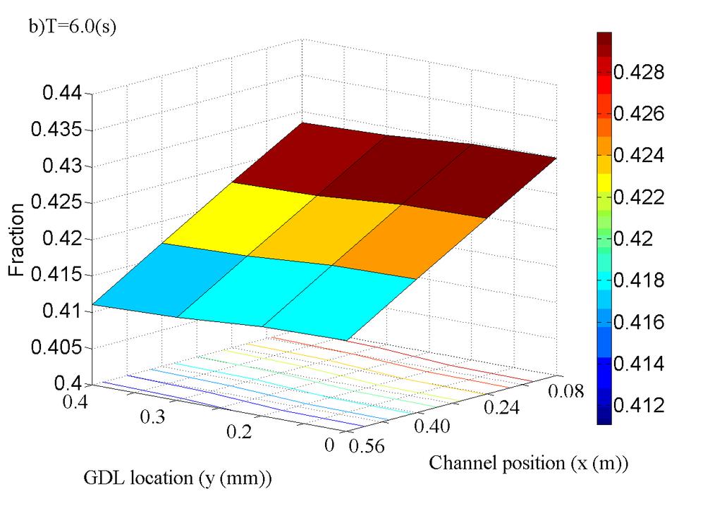
108 96

109 Figure 31 H 2 mass fraction distribution down the channel and into the depth of the GDL at a)1 b)6 and c)10 seconds - (with load profile from Figure 26) These plots show the effects of transport processes including the transport to and through the porous GDL s of both the anode and the cathode. At high i, the drops in partial pressures of the reactants due to transport losses can significantly affect V cell and thus η elec. 4.3 Stepped Voltage Another transient case that may be of interest is stepped increases in fuel cell power density. In the current study, such stepped changes in voltage were used for generating V cell -i curves under some operating condition, as well as making sure that, physically, the transience of BOP components does not damage or reduce the life of the stack. Figure 32 shows a load profile, with voltage and hydronium concentrations in both sides of the electrolyte. V cell shows quick equilibration as we might expect, 97