Quarterly Report for Contract DE-FG36-08GO Stanford Geothermal Program July-September 2009

Transcription

1 Quarterly Report for Contract DE-FG36-08GO18192 Stanford Geothermal Program July-September 2009

2 ii

3 Table of Contents 1. FRACTURE CHARACTERIZATION USING PRODUCTION DATA SUMMARY INTRODUCTION RESERVOIR SIMULATIONS WITH DISCRETE FRACTURE NETWORKS CHARACTERIZING WELL-TO-WELL CONNECTIONS DISCUSSION FUTURE WORK CONCLUSIONS FRACTURE CHARACTERIZATION OF ENHANCED GEOTHERMAL SYSTEMS USING NANOPARTICLES SUMMARY INTRODUCTION SELECTION OF NANOPARTICLES AND NANOWIRES NANOPARTICLE AND NANOWIRE CHARACTERIZATION METHODS CORE CHARACTERIZATION EXPERIMENTS NANOFLUID INJECTION EXPERIMENTS RESULTS FUTURE WORK REFERENCES 49 iii

4 iv

5 1. FRACTURE CHARACTERIZATION USING PRODUCTION DATA This research project is being conducted by Research Assistant Egill Juliusson, Senior Research Engineer Kewen Li and Professor Roland Horne. The objective is to investigate ways to characterize fractures in geothermal reservoirs using production data. 1.1 SUMMARY The Stanford University Geothermal Program has taken on a project titled Fracture Characterization in Enhanced Geothermal Systems by Wellbore and Reservoir Analysis. Part of this project involves fracture characterization utilizing advanced mathematical analysis to extract information from production data. The preceding quarterly report (March-June 2009) introduced a statistics-based deconvolution method which was used to extract core information from production data. This report discusses a different deconvolution method with a derivative-based smoothing mechanism and some additional techniques that improve the robustness of the procedure. Simulations of pressure, temperature and tracer through a discrete fracture network are presented, for two main purposes. First, the simulations provide better insight into the behavior of fluids flowing in hot fractured rocks, and our work helps clarify the extent to which current simulators can be used. Secondly, the output (synthetic data) is useful to further validate and test the deconvolution methods under investigation. Future effort will be put into improving the discrete fracture network simulations and testing the deconvolution methods with different types of data, e.g. pressure and temperature. 1.2 INTRODUCTION Some of the key questions that a geothermal reservoir engineer has to address have to do with the predicted size of the resource, and variations in productivity of wells. Further plans for development are based upon this information, e.g. the estimated size of the power plant to be built, the project lifetime and the number of wells and make-up wells required. The relationship between the wells and the resource is hard to determine because generally geothermal systems are highly heterogeneous with fracture-dominated flow. Tracer tests are commonly performed to gain an understanding of the well-to-well interaction, and various estimates can be made from the return curves. For example, the total reservoir volume and the efficiency of heat recovery can be estimated, which is very important for reducing uncertainty in volumetric Monte Carlo models. These are commonly used, for example by the USGS for the National Geothermal Resource Estimate (Williams et al., 2008) and in the early stages of geothermal project development. At later stages, tracer return curves can also be used, e.g. to predict the expected decline in production temperature with time, and the allowable increase in energy production from underutilized reservoirs, as shown by Axelsson et al. (2001). 1

6 Lovekin and Horne (1989) illustrated the usefulness of well-to-well interaction data for optimizing reinjection scheduling. The essence of the approach was to minimize the fieldwide risk of thermal breakthrough. This required an estimate of a connectivity parameter quantifying the risk of breakthrough between each injector-producer pair in the field. Multiple parameters were suggested for quantifying the connectivity, many of which would be obtained from tracer tests, e.g. initial and peak return time (t i and t p ), peak return concentration (C p ) and cumulative tracer return (f), see Figure 1.1. Given the connectivity parameter, the scheduling problem could be set up as a constrained quadratic program which was solved to find the optimal injection and production rates. Figure 1.1: A tracer return curve and some relevant measures. A drawback to the approach of Lovekin and Horne was associated with the difficulty in obtaining the connectivity data. These could be obtained by performing tracer tests for each injection well. That is, however, a nontrivial task and requires either the use of different types of tracer for each injection well, or waiting a long time (years) between tests on each individual injection well. Finding a way to determine the origins of a tracer signal based solely on the transients of the input and output is one of the goals of this work, thus allowing the application of tracer tests on multiple wells simultaneously with only one type of tracer. Situations where such data might be available could arise where natural tracers (e.g. chloride produced in brine) are being injected constantly as part of the circulation process in the geothermal power cycle. Figure 1.2 has an example of such data, collected from the Palinpinon geothermal field in the Philippines. 2

7 Figure 1.2: History of injection and produced chloride concentration in well PN-29D, in the Palinpinion field, Philippines. Macario (1991), Sullera and Horne (2001) and Horne and Szucs (2007) worked on revealing relationships between injection and production in the Palinpinon data set, with moderate success. Well-to-well correlation in the Palinpinon data could have been hard to find, because the flow conditions in the reservoir were being changed constantly, thereby altering the well-to-well flow units. Another consideration that was largely disregarded by these previous studies is that there must be a time shift between a signal generated at the injector and the corresponding response in the producer. The signal will also be subject to some degree of dispersion. The deconvolution approach discussed here takes some of these effects into account (i.e. time lag and dispersion), without assuming much else about the outcome. Similar approaches, using pressure data, have been discussed by Levitan (2007) and Lee et al. (2008, 2009). At the moment we do not have an actual data set with sufficient temporal resolution to validate the method. Therefore, synthetic data were generated using the TOUGH2 reservoir simulator. In these simulations, fractures were modeled as discrete thin blocks, which allowed us to capture some of the characteristics of tracer returns often seen in the field. 3

8 Our approach still has some limitations, e.g. predictions with the deconvolution approach depend on the flow field being close to steady state. Moreover, the matrix-to-fracture heat transfer and diffusion has not been captured well in our flow simulations. However, with some moderate improvements, this work does seem applicable to many cases, in particular Enhanced Geothermal Systems (EGS) and other liquid-dominated systems. 1.3 RESERVOIR SIMULATIONS WITH DISCRETE FRACTURE NETWORKS This chapter discusses the process of setting up flow simulations in discrete fracture networks (DFNs). An example is presented that provides insight into the behavior of pressure, temperature and tracer in fractured reservoirs and helps understand the limitations and capabilities of commonly available software Setting up a Discrete Fracture Network Reservoir Model for TOUGH2 This section describes reservoir simulations that were set up to simulate flow through fractured medium. While much of this was discussed in the quarterly report for winter 2009 it is repeated here for completeness. Discrete fractures in this work were simulated as thin rectangular blocks with high permeability and porosity. The porous ( non-fracture ) medium was broken into triangular matrix blocks which conform to the previously generated fracture network. Some numerical manipulation was required to generate a list of reasonable transmissibilities between elements, and the TOUGH2 simulator had to be slightly tricked to get the desired result as shown by McClure (2009). The simulation involves a calculation of all relevant thermodynamic properties and the mixing of water and tracer (i.e. two-waters ). The theoretical grounds for the DFN approach taken here were introduced by Karimi-Fard et al. (2003). The first step in setting up a discrete fracture network simulation was to generate a discrete fracture network. A number of software packages are available for creating these in three dimensions, e.g. FRACMAN from Golder & Associates and FRACA from Beicip-Franlab. In order to keep the exercise simple, a two-dimensional network was created in MATLAB with a code loosely based on the geomechanical process of fracture formation. Further discussion on the code can be found in Juliusson and Horne (2009a). After the fracture network had been generated, a suitable computational grid was formed. This was accomplished using the open source mesh generator Triangle, written by Shewchuk (1996). The program and all associated commands and files are well described on the Triangle website, Figure 1.3 shows a stochastic fracture network with a conforming triangular grid. The fractures were given a porosity value of 0.9 and randomly assigned a width, w, of 1.0, 0.8 or 0.6 mm; the corresponding permeability was determined by 2 w k = (1.1). 24 The matrix blocks were set to porosity 0.12 and permeability 1.0 md (10-15 m 2 ). 4

9 Figure 1.3: An example of a synthetic fracture network (red) and a mesh (blue) that conforms to the fractures. The fracture width is representative of the permeability assigned. Each of the elements created by the mesh (i.e. the triangles and fracture segments) was assigned a transmissibility to enable the use of the mesh with a general reservoir simulator. This was accomplished using a specialized computer code developed and described by Karimi-Fard et al. (2003). The transmissibility values obtained are related to the flow between two adjoining elements, i and j, as Q = T p p ) (1.2) ij ij ( j i where Q is the flow rate, T is the transmissibility, and p is the pressure in the gridblock. The TOUGH2 simulator is not equipped to handle transmissibility terms as input data. To account for that, the permeability of the gridblocks was set to 1 m 2 in the ROCKS section. Then, in the CONNE section listing the properties of element connections, the distances D1 and D2 were each set to 0.5 and the AREAX values were set equal the previously calculated transmissibility values, T ij. This way, TOUGH2 was reconfigured to perform two-dimensional horizontal simulations. To be able to take account of molecular diffusion effects, which are based on the spatial gradient (e.g. diffusion), the correct distances (D1 and D2) could have been supplied. In this case the transmissibility values should also have been modified by multiplication with D ij =D i +D j Case Study: Injection of Variable Amounts of Tracer Following is a description of a simulation case that was created to illustrate the performance of this set up. The simulation was carried out on a two-dimensional horizontal grid with dimensions 1000x1000x200 m 3. The boundaries were modeled as closed (noflow). Three injectors were configured to inject water each at 10 kg/sec with enthalpy 500 5

10 kj/kg. Two production wells were modeled to deliver against a bottomhole pressure of 30 bar with productivity index of 4x10-12 m 3 (as specified for TOUGH2). The well configuration is shown in Figure 1.4. Figure 1.4: A two-dimensional DFN simulation scenario with three injectors (IN01-03) and two producers (PR01 and PR02). The initial conditions were set to 40 bar, 230 C, and tracer mass fraction kg tracer /kg total (the tracer mass was not zero because the simulator had problems with that initial condition). Then the production was allowed to continue for about 250 days, or until the production pressure and temperature in the wells had stabilized. Figures 1.5 and 1.6 illustrate this steady state condition for pressure and temperature, respectively. The steadystate temperature found in the production wells was overpredicted because cooling of the fracture walls was not properly modeled. 6

11 Figure 1.5: Pressure distribution (steady state) for the DFN simulation scenario. Figure 1.6: Temperature distribution (steady state) for the DFN simulation scenario. A second simulation was run, starting with the steady-state conditions described earlier and the same injection and production rates. In addition to that, a small, random fraction of tracer was added to the injection stream. The modeled tracer injection and production are shown in Figure

12 Figure 1.7: Tracer injection and production history for the DFN simulation scenario. Tracer distribution at day 90 (black dashed line) is shown in Figure 1.8. The path taken by the tracer could be viewed, e.g. by feeding the simulator with a slug input into only one of the wells at a time. Further inspection of this process revealed that IN01 only feeds into PR01 and IN03 only feeds into PR02. However, IN02 feeds into both PR01 and PR02, and it is also clear that it feeds PR02 through at least two different flow paths. The return curves were also lacking the rarefaction commonly observed in tracer return curves, the reason being that the simulator would not run when molecular diffusion effects were included. An illustration of the tracer mass fraction in the reservoir at around 90 days is shown in Figure 1.8. Figure 1.8: Distribution of tracer concentration at approximately 90 days (corresponds to black dashed line in Figure 1.7). 8

13 1.4 CHARACTERIZING WELL-TO-WELL CONNECTIONS As discussed in the introduction, part of our objective is to find a relationship between the input to an injection well and the corresponding response in a production well. While minimal assumptions should be made about the outcome, the deconvolution approach assumes that the relationship is causal (time delay), linear and time invariant (flow is steady state). Moreover, we use an inversion technique that constrains the estimated response to have some degree of smoothness and be nonnegative. The following sections describe the mathematical formulation of the problem and two example applications Formulation of a multiwell deconvolution problem The method applied here is based on the assumption that well-to-well connectivity can be characterized by the convolution Equation (1.3). This implies that the production, c p (t), at one well can be described as a linear function (weighted sum) of previous injection, c r (t), into another well. The weights, κ(t), depend on the time lag between injection and production and form a curve referred to as the kernel. This curve is analogous to a tracer return curve from a slug injection tracer test (within a multiplicative constant, depending on the mass injected). p t = c ( t c ( t) τ ) κ( τ ) dτ (1.3) 0 r Equation (1.3) can be set in discrete numerical form as: r Hκ r c p = (1.4) where H is an n by m matrix, n is the number of conditioning data points and m is the number of discretization points for κ r. The kernel, κ r, is the unknown to be estimated. The elements of the H matrix representing the injection will have the formulation described by Equation (1.5), assuming a Riemann numerical integration scheme with discretization points τ = τ / 2 + ( j 1) τ j 1,...,m. j, and { } τ cr ( ti τ j ) τ, ti > τ j H = 2 ij (1.5) τ 0, ti <= τ j 2 The convolution equation can be generalized to handle the case where there are multiple (N r ) injectors, i.e. where the response in the producer is described by: c p N = r t ( t) c ( t τ ) κ ( τ ) dτ (1.6). k= 1 k = 1 0 In this case the discrete form becomes: N r = r r r c H κ = Hκ where now and p k k rk [ H H K ] H Nr k (1.7) H = (1.8) 1 2 9

14 r r r [ κ κ K ] T r κ = (1.9). 1 2 κ N r Various solution methods have been proposed to solve the convolution equations (deconvolution). We have experimented with a number of those, in particular a method discussed by Kitanidis (2009) based on Bayesian statistics. Our results for the Bayesian approach are discussed in Juliusson and Horne (2009b). The method introduced here is more in line with the work of Levitan (2007). The deconvolution problem can be particularly challenging because the H matrix has columns that are shifted versions of the previous columns. This generally means that H will be singular or very close to singular, so unfiltered solution approaches are highly susceptible to noise in the injection and/or production data. Such direct inversions often lead to highly erratic estimates of the kernel function. To counterbalance this, we introduce from physics and observations, the fact that tracer returns will have some degree of continuity (smoothness). This can be modeled by viewing the deconvolution problem as a minimization problem, where the data misfit is minimized in balance with a penalty term for the roughness in the kernel estimate. Hence, the objective function becomes r r r T r r rt r F κ 1 ( ) = 1 ( c p Hκ ) ( c p Hκ ) + κ Rκ (1.10) data misfit roughness where R denotes a roughness penalty matrix, the purpose of which is to introduce some degree of smoothness into the solution, which can be obtained through several different formulations. The approach taken here is to formulate R so as to minimize the d th derivative of the kernel function. For example, if smoothness is to be enforced by minimizing the first derivative, the roughness penalty term can be formulated as: 1 1 r m T r σ 2 κ Rκ = ( κ i+ 1 κ i ) (1.11) 2 2 i= 1 where σ is a scaling parameter that determines the emphasis on smoothness in the optimization. The first derivative approach corresponds to seeking the shortest line through the data. Similarly one can minimize the curvature of the kernel estimate, by using the second derivative, i.e. 1 2 rt r κ Rκ = σ 2 m 2 i= 1 ( κ 2 i 1 2κ i + κ i+ 1 ) penalty (1.12) In general this formulation is simply requiring there to be some correlation between consecutive elements of the kernel estimate, r κ. The d th derivative based roughness penalty term can be formulated as 1 2 r κ T R r κ = σ 2 m d d + j d ( 1) κ i j j i= 1 j= 0 2 (1.13) The general formulation of R can be found from Equation (1.13) by differentiating twice with respect to κ, i.e. where R pk d j m d k i d p i d = σ ( 1) ( 1) (1.14) i= 1 k i p i = 0, if j < 0 or j > d. (1.15) For the multiple injector case, R will be an m*n r -by-m*n r block diagonal matrix, with each m-by-m matrix block described as in Equation (1.14). The scaling parameters, σ, can 10

15 and should be tuned for each matrix block to obtain optimal results. In our experience it has worked well to select the scaling parameters as a multiple of the discretization interval for each kernel estimate, e.g. r r σ = s τ (1.16) where r σ and r τ are vectors of length N r. The scaling parameter, s, was tuned manually, but that was quite easy since only the approximate order of magnitude had to be found. A formulation of R corresponding to the second derivative was generally found to give sufficiently smooth solutions. The optimization problem specified in Equation (1.10) was solved in MATLAB using the interior-point algorithm implemented in the function fmincon, which is available in the Optimization Tool Box. The solution was constrained to be nonnegative and the initial and final elements of each kernel estimate were set equal to zero. The solution time was reduced significantly by providing the gradient: r T r r r G( κ ) = H ( c Hκ ) + Rκ (1.17) and the Hessian: for the problem. p T E(κ r ) = H H + R (1.18) Despite all of the constraints, the solution method would often fail when tested with kernel estimates that were discretized over a time scale that spanned a time greater than needed to cover the nonzero part of the kernel. Therefore, additional effort was put into estimating the final nonzero response time, t f (see Figure 1.1), for each kernel. In other words, the appropriate time scale for each estimate had to be found. It turned out that the appropriate time scale could be found by solving a second optimization problem. This time it involved finding the vector t r f which denotes the final time for the discretization of each kernel. The function being minimized is still the one described by Equation (1.10), but we are searching for the discretization interval for r κ, that gives the smallest possible F. A contour plot of F as a function of t f1 and t f2 is shown in Figure 1.9. The plot was created for a two injector case, with a random injection pattern, and using the synthetic kernels shown in Figure 1.10 to create the corresponding production data. The shape of the contour plot (Figure 1.9) can be understood in the sense that F gets large if t f is too small, since the kernel will not span a time scale large enough to explain the data misfit. On the other hand, if t f is too large, there will be fewer discretization points to characterize the nonzero part of the kernel, which leads to a poorer data fit. It could also be argued that the roughness penalty term will generally increase (and thereby F) since variations in the estimate where the kernel should be zero must be attributable to noise. Figure 1.9 also clearly illustrates that the objective function, in this context, is non-convex. That is why direct search methods were needed to solve this second optimization problem. 11

16 Figure 1.9: A contour plot of how the log of the objective function varies depending on the assumed end time (t f ) for each kernel estimate. The minimum is shown as a red star. This example was generated using the kernels shown in Figure 10. Figure 1.10: Synthetic kernels used to illustrate the dependence of the objective function (Figure 10) on the final time used in the inversion for each kernel. A direct search strategy that was found quite successful in determining the time scale was to first apply a Genetic Algorithm to find the approximate location of the minimum, and then follow up with a Pattern Search algorithm. Both of these searches were implemented with functions from of the Optimization Tool Box in MATLAB. 12

17 1.4.2 Deconvolution using DFN Simulation Data The first application example that will be discussed is the deconvolution of the synthetic data generated from the DFN simulation discussed in Section 2.2. Some Gaussian noise was added to the first 90 days of the data and then that part was used to estimate the kernels. The kernel estimates are shown in Figures 1.11 and As can be seen, injectors IN01 and IN02 have a well-characterized connection to producer PR01, while IN03 contributes very little to the signal in PR01. Note that the time scale estimate for IN03 is quite arbitrary since the kernel values are all close to zero and therefore have little effect on the objective function. Similar observations can be made for the kernels relating to PR02, where IN03 is well connected and IN01 has very limited connection. A range of other conclusions can be drawn from the shape of the return curves, about the fraction of tracer produced in each well, the travel time, level of dispersivity in the reservoir etc. Figure 1.11: Kernel estimates for connections to producer PR01. 13

18 Figure 1.12: Kernel estimates for connections to producer PR02. Note that the time scale is different from that in Figure Figure 1.13: The data for the first 90 days was used to estimate the kernels and the response for the next 90 days was quite successfully predicted, as shown here. The kernel estimates were used to predict the future response in the production wells, using Equation (1.4). The resulting predictions were quite accurate, as illustrated in Figure This serves as a type of validation for our results Deconvolution using Data from an Analytical Equation As a second example, synthetic production data were generated for a case with five injectors and one producer. The data were generated using an analytical solution of the one-dimensional advection-dispersion equation, specifically the finite impulse response on an infinite domain, i.e. 2 fm ( x ut) c p ( t) = exp (1.19) 4πDt 4Dt 14

19 where c p is the produced concentration [kg/m], f is the fraction of tracer retrieved in the producer, M is the injected mass [kg], D is the dispersivity coefficient [m2/s], x is the flow distance between the wells [m], and u is the mean flow velocity [m/s]. The relationship between mass and concentration can be written as: M = c r ( t) udt (1.20) where c r is the concentration of injected fluid and dt is the duration of the injection pulse. This can be substituted into (1.19) to obtain any given response by convolution: t 2 fcr ( t τ ) u ( x uτ ) c p ( t) = exp dτ (1.21). πdτ 4Dτ 0 4 So in this case the kernel has the formulation: 2 fu ( x ut) κ ( t) = exp (1.22). 4πDt 4Dt Note that the kernel depends only on the characteristics of the well-to-well connection, and not the mass or concentration of tracer injected. The kernel is however dependent on the amount of injected fluid, through the average flow velocity, u. This means that meaningful kernel estimates require that the fluid injection and production rates stay constant (or close to constant), but the amount of injected tracer can and should vary. Taking this analytical approach has several advantages for validating our method, for example we can (easily) generate a large variety of kernels, and the true shape of the kernels will be known a priori. The deconvolution method was subject to a slightly harder test this time as the number of injectors was increased to five. Each of the five injectors had an arbitrary connection to the producer as illustrated in Figure Figure 1.14: Set up with one producer and five injectors. The connecting path to the producer is unknown. 15

20 Figure 1.15 shows the kernels associated with each injector-producer connection. Importantly, these illustrate a fair amount of variety in dispersivity, retrieval fraction, flow velocity and distance. Figure 1.15: Five synthetic kernels used in this example Each kernel in our estimate was discretized into 50 elements. This means that the total number of parameters being estimated was 250. The production data generated in this case contained 400 measurements. Therefore, it was very important to have as little redundancy as possible in the convolution equations, i.e. the output signal had to contain as much information as possible about the response of the producer to changes at each injector. To accomplish this, an approach, similar to that presented by Lee et al. (2008, 2009), was taken, which involved creating a series of Haar wavelet based injection signals. This way a wide combination of injection signals was tested and all injectors received the same total amount of tracer, but in varying concentration over varying time spans. Figure 1.16 illustrates the tracer injection pattern used, and the corresponding output signal. 16

21 Figure 1.16: Controlled injection and corresponding production for a case with five injectors and one producer. The deconvolution method described in Section was used to solve this five injector case. As Figure 1.17 shows, a solution was found that reproduced the data very well. Moreover, all of the kernels (which were known in this case) were reproduced quite accurately. This is illustrated in Figure Note that the inversion worked well even though the time scale (time beyond which the kernel essentially goes to zero) was a bit off in a few cases, e.g. for kernels 3 and 5. Figure 1.17: Data reproduction after solving the five injector case. Figure 1.18: Estimated kernels compared to actual kernels used. Admittedly, the inversion was less robust when some of the kernels were extremely dissimilar, especially for kernels that were highly dispersive or if the fraction of tracer retrieved was very small, since the contribution of these to the signal would be negligible 17

22 or lost in noise. On the other hand, the high uncertainty associated with those kernel estimates could possibly be quantified and linked to low connectivity between wells. 1.4 DISCUSSION An important observation should be pointed out regarding the limitations of tracer tests. The DFN simulation presented in Sections and (and this was verified by further simulation) showed that well IN01 sent tracer only to well PR01 and none to PR02. Similarly, tracer from IN03 was only produced in PR02. The kernel estimates also revealed this information. Note, however, that the tracer returns do not say anything about which wells are not connected. For example, it is clear from the DFN model that there is a fracture connection between IN03 and PR01, but that is not seen in the tracer returns because of the specific operating conditions in our model. It should also be reiterated here, that the reason the deconvolution method works so well in here is that the model conditions set up in this case involved steady state pressure and temperature. The only thing that was varied was tracer concentration, which at these conditions gives a linear response. These conditions are somewhat idealized, but conditions that are very close will surely occur, especially in EGS and other liquid dominated systems. A real data set that would help illustrate the usefulness of this approach has not been found, and it seems unlikely that a data set with sufficient temporal resolution exists. Therefore, the take-home message is that collecting chemical samples more regularly (daily) may be worth the effort. Moreover, a well controlled injection schedule will make the method more likely to succeed. 1.5 FUTURE WORK The discrete fracture network models introduced here clearly need some refining. One of our near future goals is to implement diffusion. This will hopefully yield more realistic tracer return curves. Simulations of heat transfer between the fracture and adjoining matrix blocks also need to be improved. Finally some testing of three-dimensional models could be carried out. This deconvolution method should be extendable to other data types, e.g. pressure, temperature and enthalpy, and those will be considered in future research. The information conveyed by the kernels should also be useful for characterizing the fracture network that created them. Given a compatible data set, we will also put effort into proving the validity of these deconvolution methods. 1.6 CONCLUSIONS Research during summer quarter of 2009 has focused on multiwell deconvolution of tracer production data and simulations of tracer tests in discrete fracture network models. 18

23 A two-dimensional reservoir model with a discrete fracture network was built and used for numerical simulations with the TOUGH2 code. A case study of tracer injection, with three injectors and two producers, was presented. One important lesson learned from the simulations was that tracer returns can give information about which wells are connected, but they can not be used to make conclusive remarks about which wells are not connected through a fracture network. Otherwise, some of the DFN simulation capabilities and limitations were discussed. For example, heat and solute transfer effects between the fracture and the matrix need to be captured more effectively. A formulation of the deconvolution problem for tracer returns was presented. The formulation included the multiple-injector single-producer case. The method was then used to solve two examples, based on synthetic tracer data. The results indicate that this deconvolution method can successfully reveal the underlying transfer functions (kernels) for tracer transport between wells. The kernels are analogous to tracer return curves and can therefore be used to make any predictions made from conventional (slug injection) tracer tests. The kernels can also be used to predict the response to future variations in the injection of solute. It is important, however, that the flow field remains at steady state (roughly) throughout the data collection and prediction period. Future work will be divided into improvements of the current DFN simulation methods and experimentation with deconvolution using different types of data. 19

24

25 2. FRACTURE CHARACTERIZATION OF ENHANCED GEOTHERMAL SYSTEMS USING NANOPARTICLES This research project is being conducted by Research Associate Mohammed Alaskar, Senior Research Engineer Kewen Li and Professor Roland Horne. The objective of this study is to investigate the possibility of using nanotechnology to characterize the fracture system (direction, shape and size of fractures) in Enhanced Geothermal Systems (EGS). 2.1 SUMMARY A trial nanoparticle injection into Greywacke sandstone was completed. Silicon Oxide (SiO 2 ) nanoparticles were flowed through a Greywacke sandstone core from The Geysers. Distortion of nanoparticle shape was observed in several effluent samples. The particles have either a cut in a single side or an unusual appearance. Due to the ambiguity in the results, the experiment will be repeated for verifiability purposes. An attempt to transport silver nanowires through Berea sandstone pore network was carried out. The silver nanowires did not make their way through the core. The nanowires were found to be trapped at the inlet. Scanning Electron Microscopy (SEM) imaging was used to reach this finding. Prior to the nanoparticle and/or nanowire injection experiments, the Greywacke and Berea sandstone cores were fully characterized. The gas and liquid permeabilities, porosity and pore size distribution of the core samples were measured. This report describes nanoparticle and nanowire characterization methods, details of permeability and pore size distribution measurements, and results of the nanoparticle and nanowire injection experiments into Greywacke and Berea sandstone core samples, respectively. 2.2 INTRODUCTION Last quarter (April-June 2009), a trial nanoparticle injection into a rock core was completed successfully. Silicon Oxide (SiO 2 ) nanoparticles were flowed through a Berea sandstone core. The injected nanoparticles were transported through the pore space of the rock and were detected in the effluent. In this quarter, preliminary testing of different core samples and nanofluids was continued. For instance, the injection of SiO 2 nanoparticles into a Greywacke core was conducted. Greywacke sandstone is a very low permeability rock typical of geothermal reservoirs and therefore initial experimentation with it was indicative. An attempt to injection silver nanowires into a Berea sandstone core was also carried out. Analytical details of both experiments are included in Section 2.7 of this report. Standard measurements on the core samples were also performed. These measurements included the gas and liquid permeability, porosity and pore size distribution measurements. 2.3 SELECTION OF NANOPARTICLES AND NANOWIRES Nanoparticles and/or nanowires used in this study, and ultimately in the reservoir, need to be safe to handle and environmentally friendly (Kanj et. al., 2008). Monodisperse silica 21

26 nanoparticles (silicon oxide, SiO 2 ) and silver nanowires (AgNW) satisfy all essential requirements and therefore were selected for initial experimentation. The SiO 2 nanoparticle preparation was accomplished by the hydrolysis of tetraethyl orthosilicate (TEOS) in aqueous ethanol solutions containing ammonia (Bogush et al., 1988).The SiO 2 nanoparticle preparation details are found in first quarterly report (January-March 2009). Nanoparticles injected were in the size range of 70 to 450 nm. A distribution of sizes was accomplished by mixing 1, 0.3 and 0.2 ml of 70, 200 and 450 nm nanoparticles, respectively. Silver nanowires were readily available from the Nano Characterization Laboratory of Stanford University. The silver nanowires injected had diameters in the range of nanometers, and lengths in the range between 5-10 micrometers. The conditions for the preparation of the uniform silver nanowires follow, for the most part, the study by Sun et al. (2002). The formation of silver nanowires is accomplished by reducing silver nitrate (AgNO 3 ) with ethylene glycol (EG) in the presence of silver (Ag) seeds. Polyvinyl pyrrolidone (PVP) is then added to direct the growth of silver into uniform nanowires. The longitudinal and lateral dimensions of the silver nanowires are controlled by changing the reaction conditions. Sun et al. (2002) reported that increasing the reaction temperature resulted in the formation of shorter nanowires. This synthetic method could provide uniform nanowires with high yield under environmentally friendly conditions and relatively low temperatures 2.4 NANOPARTICLE AND NANOWIRE CHARACTERIZATION METHODS In general, the quantity of the nanotracer produced at the sampling point (core exit) should be sufficient to be recognizable and at concentrations above the lower detection limit of the devices used to analyze the effluent by at least factor of three. Therefore, characterization of the rock as well as the nanofluid prior to and after injection was carried out by various techniques, as applicable. Dynamic Light Scattering (DLS) and Ultraviolet-visible Spectrophotometry (UV-visible Spectrophotometry) were used to detect the nanoparticles and nanowires, respectively. Scanning Electron Microscopy (SEM) and Optical Microscopy were also utilized to confirm the findings Dynamic Light Scattering (DLS) DLS is a technique used to measure sizes of particles suspended in liquid. The technique basically measures the random motion of suspended particles resulting from the bombardment of surrounding solvent molecules. This movement is known as Brownian motion. When particles are illuminated with a laser, the scattered light intensity varies depending on the size of the particles and hence their Brownian motion ( n.d.). These changes in light intensity are related to particles size using the Stockes-Einstein relationship given by: kt d( H ) = (2.1) 3πηD d is hydrodynamic diameter, D is translational diffusion coefficient, k is Boltzmann s constant, T is absolute temperature and η is viscosity. where: ( H ) 22

27 DLS was utilized to determine the particle size and distribution qualitatively in the injected nanofluid and the effluent samples. The measurements were performed using the Zetasizer Nano ZS manufactured by Malvern instruments. This device can detect particles as small as 0.6 nanometers Ultraviolet-visible Spectrophotometry (UV-visible Spectrophotometry) UV-visible spectrophotometry involves the spectroscopy of photons in the UV-visible region which means that it deals with light in the visible, near-ultraviolet and near-infrared ranges. The spectrophotometer is the instrument used to measure the light intensity as a function of the wavelength of the light. The Beer-Lambert law is used to determine the concentrations of absorbing species in solution quantitatively. This law states that the absorbance of a solution is directly proportional to the path length through the sample and the concentration of absorbing species in solution. The Beer-Lambert law is given by: ( I I ) = cl A = log 10 / o ε (2.2) where A is the measured absorbance, I is the intensity of light passing through the sample, I o is the intensity of light before it passes through the sample, L is path length through the sample, and c is the concentration of absorbing species. ε is the molar absorptivity constant which is specific for each species and wavelength at particular temperature and pressure and which has units of AU / M * cm. Therefore, by knowing the path length of the sample along with the absorptivity constant and measuring the absorbance of the substances in solution, the concentration of the substance can be calculated easily. The Beer-Lambert law implies that there is an equal effect of the changes in concentration and path length. For example, dilution of the sample by factor of 12 would have the same effect on absorbance as reducing the path length of the sample (cuvette) from 12 to 1 millimeter. This technique was used to characterize the injected silver nanowires only. The UV-visible absorbance spectra were taken at room temperature using a Shimadzu UV-1700 spectrophotometer using a 12 mm square polystyrene cuvette. All samples were sonicated prior to analysis. Some had been diluted 2x with deionized water before taking spectra while others were analyzed without dilution. The morphological evolution involved in the growth process of the silver nanowires was explored extensively by Sun et al. (2002). Figure 2.1 shows the typical absorbance spectra of the silver nanowires at different reaction times. This could be considered as the optical signature of relatively long nanowires. The increase in intensity of the two surface plasmon resonance (SPR) peaks at 350 and 380 nm (from curve k to m) is indicative of the further elongation of the silver nanowires and increase in the number of nanowires formed as the reaction completed at 60 minutes. The concentration of the nanowires in the sample is in direct relation to the absorbance level at those peaks. For instance, the absorbance levels at 23

28 350 and 380 nm peaks had increased roughly twofold as the reaction continued (curve k to m of Figure 2.1). Figure 2.1: UV-visible absorbance spectra of the reaction mixture at different reaction times (adopted from Sun et al., 2002) Optical Microscopy Optical Microscopy was used in this study mainly for the identification of silver nanowires. A Nikon Eclipse E600 POL optical microscope equipped with Polaroid digital camera (Figure 2.2) was utilized to capture optical images. The sample requires no special preparation except for placing a drop of the solution on a glass cell, however, sample observation under the microscope can be time-consuming. Although optical microscopy is convenient and simple, measurements of nanowire size (length and diameter) obtained are not very accurate and therefore Scanning Electron Microscopy (SEM) or Transmission electron microscopy (TEM) are recommended for size measurements. This is has to do with the polarizing microscopy technology itself. When polarized light (created by passing light through a polarizing filter) interacts with a material, the incident light could provide information about its structure. This is based on the fact that most solid materials have optical properties that change with polarized light reflection direction. Thus, as materials rotate, we may observe, for example, brightness or color change under polarized light. Such changes could then be related to certain materials ( n.d.). Nevertheless, optical imaging can serve the purpose of identification (existence) of nanowires in the sample under investigation. 24

29 Figure 2.2: Polarized light microscopy from Nikon (adopted from Scanning Electron Microscopy (SEM) Microscopy-based techniques for particle size characterization provide a powerful tool for characterization of particle size, size distribution and morphology. A major advantage of the microscopy-based technique is the ability to identify the particle shape (Jillavenkatesa et al., 2001). This is particularly important in the nanofluid injection experiments because it enables us to distinguish the recovered nanoparticles from preexisting objects such as rock fines and debris. The measurements were performed using a Philips FEI XL30 Sirion SEM instrument with Field Emission Gun source at the Stanford Nano Characterization Laboratory. As mentioned earlier, SEM imaging is useful to confirm the DLS and UV-visible Spectrophotometer measurements which are simpler and cheaper but which do not distinguish between the particles other than by size. Moreover, SEM was used to study the nanoparticle placement inside the rock matrix and how they arrange themselves in the pore spaces. In this regard, three different slices of the core at inlet, outlet and middle were cut and prepared for SEM analysis (Figure 2.3). Elaboration on the results is included in Section 2.7 of this report. 25

30 Figure 2.3: Rock sections of Greywacke sample for SEM analyses 2.5 CORE CHARACTERIZATION EXPERIMENTS This section provides the details of the first attempt to inject silicon oxide (SiO 2 ) nanoparticles and silver nanowires (AgNW) into Greywacke and Berea sandstone core samples, respectively. Prior to nanofluid injection, standard experiments to characterize the rock cores were performed including the pore size distribution and permeability measurements. Specification and calibration of all equipment and hardware used in these experiments can be found in the first quarterly report (January-March 2009). These include pressure differential and mass flow rate transducers, water and vacuum pumps and weight balance Greywacke Core Characterization The core sample tested was a Greywacke sandstone of 3.8 centimeters diameter and 5.6 centimeters length. The pore size distribution of the core sample was measured by the mercury (Hg) intrusion method. The intrusion of mercury was performed using the AutoPore IV 9500 Mercury Porosimeter manufactured by Micromeritics. The measurement procedure and methodology can be found, with greater detail, in the last quarterly report (April-June 2009). Measurements conducted on the Greywacke sandstone showed the core to have a porosity of about 6% and pore sizes as large as 150 nanometers (Figure 2.4). The gas and liquid permeabilities were determined. The Klinkenberg (gas slippage) effect was considered to evaluate the equivalent liquid permeability. Then, the liquid permeability for the same core sample was carried out. Porosity and permeability results are summarized in Table

31 ential intrusion of Hg (ml/g/µm) Figure 2.4: Pore size distribution of Greywacke rock from The Geysers Table 2.1: Greywacke porosity and permeability measurements summary Property Measurement method Value Porosity (%) Porosimeter-mercury intrusion 6 Saturation with deionized water 4 Gas permeability 0.84 Permeability (µd) Equivalent liquid permeability 0.7 Liquid permeability Figure 2.5 is a schematic of the apparatus used in the measurement of gas permeability. The gas flowed in this experiment was Nitrogen (N 2 ). The inlet and outlet pressures were measured using standard pressure gauges. The flow rate at the outlet was measured using a stop-watch and graduated cylinder (the standard method of measuring the flow rate). Calibration curves were included in the first quarterly report (January-March 2009). 27

32 Figure 2.5: Schematic of the apparatus for measuring gas permeability. The core was first dried in a furnace at 100 o C under vacuum for 24 hours. After weighing the core sample, it was placed inside the core-holder under a confining pressure of 1000 psig. The gas permeability measurement was then started by introducing Nitrogen at different flow rates and inlet pressures. The average gas permeability was found to be around 0.84 microdarcy by applying Darcy s law for compressible fluids which is given by: k gas = 2µ p 2 A( p in qoutl 2 p ) out out (2.3) where µ is the viscosity in centipoises, q tot is outlet volumetric flow rate in cubic centimeter per second, A is the core cross-sectional area in square centimeter, L is the core length in centimeter and p in and p out are inlet and outlet absolute pressures in atmospheres, respectively. The gas permeability as a function of the reciprocal of mean pressure is depicted in Figure 2.6. According to the Klinkenberg effect, extrapolating the straight line to infinite mean pressure (or zero reciprocal of mean pressure) intersects the permeability axis at a point designated as the equivalent liquid permeability (Amyx et al., 1960). In Figure 2.6, the average equivalent liquid permeability is approximately 0.7 microdarcy. 28

33 1.0E-03 Gas permeability (md) 9.0E E E E E E E E E-04 y = x E Recipocal pressure (atm^-1) Figure 2.6: Greywacke core gas permeability versus the reciprocal of mean pressure The liquid permeability was measured on the same core sample directly. A schematic of the apparatus used in the measurement of liquid permeability is shown in Figure 2.7. Figure 2.7: Schematic of apparatus for liquid permeability measurement The core sample was first saturated with water outside the core-holder. The core and related system were evacuated using a Welch Vacuum Pump for 4 hours at a vacuum pressure of about 30 millitorr to remove moisture. Distilled water was introduced to completely submerge the sample. The core was then left submerged overnight and the remaining vacuum released to aid the process of saturation. After that the core was removed and wiped dry to remove excessive water on the surface. Finally, the core was weighed and hence its porosity was calculated. The core turned out to have a porosity of around 4 % and a pore volume of 2.19 cubic centimeters. The porosity calculation is as follows: 29

34 Vp φ = *100 (2.4) V V p B = W W (2.5) s V B 2 where φ is the porosity in percentage, centimeter, respectively. Ws and d = πr l (2.6) Vp and V B are pore and bulk volumes in cubic W d are the weight of core after and before saturation, in gram, respectively. r and l are the radius and length of the core in centimeter, respectively. The weight measurements of the sample are provided in Table 2.2. Based on these measurements, the density of the Greywacke core was found to be 2800 kg/m 3. This is in good agreement with a reported value of 2700 kg/m 3 in the literature (Tayler et al., 1982, Mossop and Segall, 1997). Again, the upstream and downstream pressures in the core as well as the confining pressure were measured by the same standard pressure gauges used previously in the gas permeability measurement experiment. In addition, a water pump was used to inject distilled water and the flow rate measured using a stop-watch and a Mettler balance (Model PE 300). The pump calibration curve can be found in the first quarterly report (January-March 2009). Table 2.2: Greywacke weight and density measurements summary Property Value Dry sample weight (gram) 60.2 Density (Kg/m 3 ) 2700 Density-calculated (Kg/m 3 ) 2800 Error in density (%) 3.7 The average liquid permeability was found to be around microdarcy. Darcy s law for horizontal flow was utilized to compute the permeability. Darcy s law for horizontal flow is given by: q L k liq = µ (2.7) A p where q is the volumetric flow rate in milliliter per second, µ is the viscosity in centipoise, L and A are the length and the cross-sectional area of the core in centimeter and square centimeter, respectively. p is the differential pressure across the core sample in atmospheres. 30

35 2.5.2 Berea Sandstone Core Characterization The core sample was a Berea sandstone 3.8 centimeters in diameter and 5.8 centimeters in length. Generally, the pore size distribution, porosity and permeability measurements were conducted in the same fashion as explained in Section Measurements performed on the Berea sandstone showed the core to have pore sizes as large as 20 micrometers (Figure 2.8). Recall that the silver nanowires intended for injection measured 10 micrometers (at most) in its longitudinal axis. Thus, theoretically, most of the nanowires should be able to turn around inside the largest pores. Porosity and permeability results are summarized in Table Diff. Intrusion of Mercury (ml/g/µm) Pore Diameter (µm) Figure 2.8: Pore size distribution of Berea sandstone core Table 2.3: Berea sandstone porosity and permeability measurements Property Measurement method Value Porosity (%) Porosimeter-mercury intrusion 19 Saturation with deionized water 18.2 Gas permeability 131 Permeability (µd) Equivalent liquid permeability 85 Liquid permeability 94 31

36 The apparatus used in the measurement of gas and liquid permeabilities was similar to the one used for the Greywacke core (Figure 2.5/2.7) except that the inlet and outlet pressures were measured using pressure transducers of different diaphragm ratings. The average gas and liquid permeabilities were found to be around 131 and 94 millidarcy, respectively. The gas permeability as a function of the reciprocal of mean pressure is shown in Figure 2.9. with average equivalent liquid permeability of approximately 85 millidarcy. 145 Gas permeability (md) y = 65.65x R 2 = Reciprocal mean pressure (atm^-1) Figure 2.9: Berea sandstone gas permeability versus the reciprocal of mean pressure Based on the resaturation of the sample, the core had a porosity of 18.2 % and a pore volume of about 12 cubic centimeters. These measurements were confirmed by calculation of the density of the Berea sandstone core. The density was computed and found to be 2.61 gram per cubic centimeters. Table 2.4 is a summary of the results. Table 2.4: Berea sandstone weight and density measurements Property Value Dry sample weight (gram) 141 Density (g/cm 3 ) 2.63 Density-calculated (g/cm 3 ) 2.61 Error in density (%) 5.2 Following the resaturation, the liquid permeability was measured by injecting distilled water using a water pump. Several flow rates were used to calculate the liquid 32

37 permeability, ranging from 1.5 to 15 milliliter per minute at different differential pressures. As mentioned earlier, the average liquid permeability was found to be around 94 millidarcy. Various estimated permeability values are plotted against the flow rate in Figure A slight reduction was observed in the permeability measurements as the flow rate increased Flow rate (cu. cm./sec) R 2 = Permeability K (md) Figure 2.10: Berea sandstone liquid permeability measured at different flow rates. 2.6 NANOFLUID INJECTION EXPERIMENTS During this quarter, two main experiments were conducted with two distinct and specific objectives. They serve as preliminary testing of the injection of various nanofluids (nanoparticles and nanowires) into different cores of distinctive characteristics (Greywacke and Berea sandstones). The injection process and sampling strategies in both experiments were similar, however, they differ in some aspects such as total Pore Volume Injected (PVI), flow rates and sampling frequency. The following sections provide, in reasonable detail, the specifics of each experiment Silicon Oxide (SiO 2 ) Nanoparticle Injection Experiment into Greywacke Core To explore the possibility of using the nanoparticles to characterize the fractures, an experimental investigation was initiated to assess a suitable particle size and to verify their transport through a very tight formation rock such as Greywacke from The Geysers geothermal field. A schematic of the apparatus is shown in Figure Nanofluid solution was contained in a pressure vessel downstream of the water pump. Due to the high differential pressure required to displace the fluid, the vessel containing the nanofluid was pressurized using the water pump (not Nitrogen gas). The configuration also allows for injection of particle-free water, without interrupting the flow. This experiment did not consider the temperature effect, so it was conducted at room temperature. The nanofluid contained silicon oxide (SiO 2 ) particles of wide size 33

38 distribution between 70 and 450 nanometers. It is of interest to inject the nanoparticles with a variation of size and determine which sizes come out in the effluent. Figure 2.11: Experimental apparatus for nanofluid injection into Greywacke core from The Geysers. Prior to the injection of the nanofluid, the core was preflushed with pure water to displace as much rock fines and debris as possible (7 pore volumes [PVs] in this case). The nanofluid injection sequence was similar to the process suggested by Kanj et al. (2008). The sequence involved the injection of a pore volume of nanofluid followed by a continuous injection of pure water. The pore volume was determined as outlined in Section In particular, two pore volumes plus the dead volume (the volume of the tubes and fittings) were injected. The dead volume is required to fill the tubes completely prior to nanofluid entering the core. Following that is the first pore volume which should fill the pore spaces. The second pore volume is used to confirm the filling. Based on the straightforward volume calculations outlined below, the pore and dead volumes were found to be 2 and 3 milliliters respectively. V p = V B φ (2.8) V inj d = πr l (2.9) p 2 t t V = V + V (2.10) d where r t and l t are the radius and length of the tube in centimeter, respectively. V d and V are the dead and total injected volumes in cubic centimeter, respectively. The rest of inj parameters have their usual definition. 34

39 Subsequent to the injection of the nanofluid (pore and dead volumes), a continuous flow of pure water (post injection) was introduced. Specifically, 10 pore volumes of pure water were injected while the effluent samples were collected. The total time of the experiment was approximately 30 days. The injection was at the rate of one milliliter per day at a differential pressure of about 700 psig. The injection pressure was kept at that level due to the limitation of the maximum allowable confining pressure of the core-holder (1000 psig). A total of 30 effluent samples were collected at the rate of one milliliter per sample. Not all these samples were analyzed but rather a careful selection of some was done to optimize the analysis time. The infrequent samples could indicate the trend of the returning nanotracer and more details (if needed) could be obtained by analyzing the samples in between Silver Nanowire Injection Experiment into Berea Sandstone Core Transporting a wire-like nanoparticle through the pores of a rock core was the objective of this experiment. For that, silver nanowires were injected into Berea sandstone. The same coreflooding apparatus (Figure 2.11) was used except that the nanowires were injected with the aid of Nitrogen gas. A schematic of the modified apparatus is illustrated in Figure Figure 2.12: Experimental apparatus for nanofluid injection into Berea sandstone The core was preflushed with 12 PVs of pure water. One pore volume plus the dead volume (the volume of the tubes and fittings) of nanofluid were injected. The pore and dead volumes were found to be 12 and 8 milliliters respectively. Subsequent to the injection of the nanofluid (pore and dead volumes), a continuous flow of pure water (post injection) was introduced. Specifically, 30 pore volumes of pure water were injected while the effluent samples were collected. The total time of the experiment was approximately 6 hours. The injection of the nanofluid was at the rate of 1 ml/min to facilitate the sampling operation. The post injection of pure water was at different flow rates. Namely, the first 7 pore volumes were injected at the rate of 0.5 ml/min, the next 12 pore volumes at the rate of 1 ml/min, the last 11 pore volumes at rate of 3 ml/min. The variation of injection rate was made intentionally to push the stuck nanowires inside the pores. A total of

40 effluent samples were collected, with volumes ranging from 1 to 6 milliliters. Less frequent sampling was performed toward the end of the injection. Several samples were selected for initial analysis. 2.7 RESULTS The injection of silicon oxide nanoparticles was aimed at testing the feasibility of transporting nanospheres through the pores of the Greywacke core as it represents the kind of tight rocks found in geothermal reservoirs. The experiment was intended to bracket the size limits of the nanoparticles able to flow through the pores. The second experiment was carried out using wire-like nanoparticles. Silver nanowires were injected through the Berea sandstone core. The objective of this experiment was to verify the likelihood of transporting rod-like nanowires through the tortuous pore network of typical reservoir formation rock. Discussion of the results is found in Section Greywacke Experiment Results Silicon Oxide (SiO 2 ) nanoparticles were identified in some of the effluent samples but not all. The interior of the rock itself was also examined. There were no signs of the injected nanoparticles. The SiO 2 nanoparticles had a wide distribution of size between 70 to 450 nanometers. Figure 2.13 is an SEM image of the original nanofluid prepared for this experiment. The nanofluid was a mix of 1, 0.3 and 0.2 milliliter of 50, 200 and 450 nm nanoparticles, respectively. The intention was to have fewer of the big particles and this was achieved. The big white spheres are the large particles ( nm) and the background is the smaller size (70 nm) particles. The nanoparticles are as expected in terms of shape, namely perfect spheres. A B B Figure 2.13: (A) SiO 2 nanospheres in the injected nanofluid, (B) Close-up image DLS analysis of the original nanofluid injected was also performed. The size distribution based on reflected light intensity is depicted in Figure DLS analysis confirms qualitatively the bimodal distribution of the injected nanofluid sample. 36

41 Intensity (% ) Particle size (nm) Figure 2.14: Bimodel distribution of injected SiO 2 nanofluid As mentioned earlier (Section 2.6.1), the injection into the Greywacke core was conducted in the following fashion. The core was first preflushed with deionized water, then the nanofluid was injected. Following that, several pore volumes of deionized water were postinjected. Figure 2.15 shows SEM images of the particle-free deionized water (preflush) evaporated solution placed on silicon substrate. It appears that all the white colored material is rock fines and debris. No signs of any round particles are seen, which is expected because no introduction of the nanofluid had taken place yet. This confirms that core fines are not round in shape and should not be confused with SiO 2 nanoparticles. In other words, any spherically shaped objects should be interpreted as injected SiO 2 nanoparticles. This gives confidence in the characterization of the effluent samples throughout the experiment as well as in the rock pore spaces itself. A B Figure 2.15: Core fines and debris in preflush effluent sample The analyses of selected, but representative, effluent samples were continued. Dynamic light scattering DLS did not work with any of the effluent samples. Many factors such as presence of dust and aggregates or high concentration of particles in solution may have made the samples unsuitable for DLS measurements. Samples were filtered using 0.8 and 37

42 0.2 micrometer syringe filters and/or diluted in order to eliminate these causes, however, the samples remained unsuitable for the analysis. This has not given big attention at this time because the more precise characterization approach (SEM imaging) was readily available. Therefore, subsequent effluent samples were analyzed by SEM imaging only. Images in Figure 2.16 were taken in a sample collected during the injection of the original nanofluid. The images have no sign of nanoparticles. That was not very surprising because the nanoparticles could be trapped initially within the rock pores and pore throats. As more deionized water was introduced (post injection), the nanoparticles started to mobilize and were produced. Perfect nanospheres were identified in the effluent of the first post-injected pore volume (Figure 2.17). Nevertheless, the irregular shapes of the smaller size particles (Figure 2.16 (B)) in the order of 10 nanometers has triggered an interesting hypothesis. It has been suggested that the nanoparticles are crushed under high pressure (700 psig in this case). If this is the case, it might be difficult to distinguish between broken pieces of the nanoparticles and core fines using this type of analysis (SEM imaging). Thus, a pressure test on a sample of nanofluid containing 350 nanometers silicon oxide nanoparticles was conducted outside the core. A B B Small particles Figure 2.16: (A) Effluent sample during injection of nanofluid, (B) Close-up image 200 nm Figure 2.17: Effluent sample of first post PVI, the scale is 200 nm A few milliliters of pure nanofluid with particles in the size range of 350 nanometers (Figure 2.18) were pressurized outside the core (in a clean container). The maximum 38

43 pressure was 2000 psig applied in steps of 500 psig at a time. At each step, a sample was collected and prepared for SEM analysis. Figure 2.18: Nanofluid used in the pressure testing To optimize the analysis time, SEM imaging was performed at the highest and second highest pressure samples (i.e. samples pressurized to 1500 and 2000 psig). The silicon oxide nanoparticles did not exhibit any distortion or damage. Figure 2.19 shows SEM images of evaporated solution of the two samples subjected to 1500 and 2000 psig. A B Figure 2.19: SiO 2 nanoparticles subjected to pressure (A) at 1500 psig, (B) at 2000 psig. It should also be mentioned that this test did not take into consideration the effect of the transport through the tortuous paths within the rock pore network. It may be possible that elevated pressure level along with the collisions of the particles as they transport through winding path, could cause particle damage. A sample at the fifth post injected pore volume shows unusual particles shapes (Figures 2.20 and 2.21). The nanoparticles appear to be round in shape on one side while having a cut from the other side. The size of these particles corresponds to the size of injected nanoparticles. In addition, the roundness of these particles from most sides suggests strongly that these are not core debris but the injected nanoparticles themselves. The distortion of the nanoparticles could not be explained at the moment. 39

44 A B B Broken spheres Figure 2.20: (A) Effluent sample at the fifth post injected pore volume showing SiO 2 nanospheres with broken side, (B) Close-up image A Unusual appearance B Distorted Nanoparticles Figure 2.21: SEM image showing SiO 2 nanospheres, (A) Unusual Appearance, (B) Distorted. The interior of the rock itself was examined. Specifically, inlet, middle and outlet slices were examined most closely. Figure 2.22 shows an SEM image of the pore spaces at all three sections of the core. The SiO 2 nanoparticles are not visible. The core has many fines and debris which makes it difficult to spot the nanoparticles. This preliminary experimentation with the Greywacke core involved several uncertainties. The unusual shape and distortion of the nanoparticles were identified at various pore volumes. The particles either have a cut in a single side (Figure 2.20), unusual appearance or distortion (Figure 2.21). The reasons for this are not known. Due to these ambiguities in the results, the experiment will be conducted again for repeatability and verifiability purposes. 40

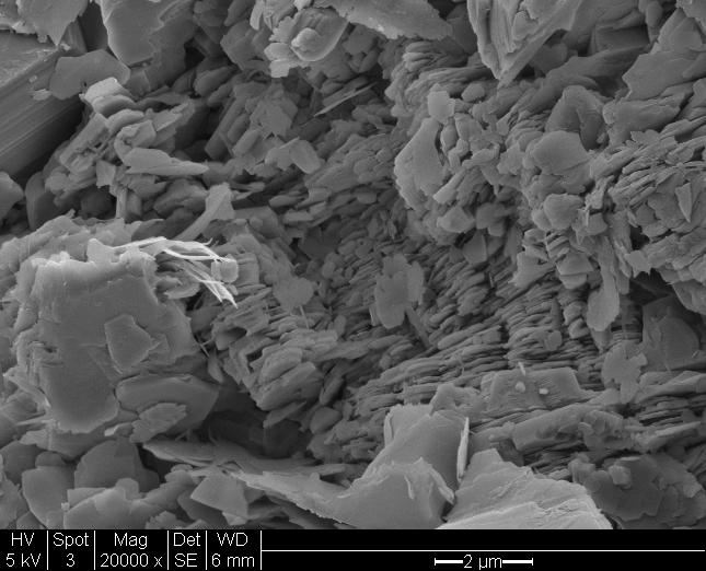
45 A B C D Figure 2.22: SEM images of the pore spaces of Greywacke core sections at, (A) Inlet, (B) Middle, (C) and (D) Outlet Berea Sandstone Nanowires Injection Experiment Silver nanowires were injected through the Berea sandstone core, however, were not detected in the effluent. The samples were analyzed and/or characterized using the UVvisible spectrophotometry and optical imaging. The silver nanowires injected had optical signature (UV-visible spectra) very similar to typical silver nanowires reported in literature (Figure 2.1, curve (m)) as depicted in Figure The size of the nanowires was nm in diameter, and 5-10 µm in length. 41

46 Absorbance Original AgNW- Prior to Inj Wavelength - nm Figure 2.23: UV-visible spectra of injected silver nanowires The size of original silver nanowires was confirmed by optical microscopy imaging. Figure 2.24 is an optical image of the injected nanowires. As mentioned earlier, more accurate measurements of sizes may be obtained from SEM/TEM microscopy. Ag-NW Figure 2.24: Optical image of the silver nanowires originally injected The effluent samples, were examined for the existence of the nanowires. Among the 139 samples collected, several samples were selected strategically. Initially, the analysis was performed on six samples. One sample from the pore volume collected during the injection of the nanofluid and others from subsequent injection (post-injection) of pure water, namely first, second, third, sixth and thirteenth pore volumes. The UV-visible spectra of these samples were taken as depicted in Figure

47 Absorbance Original AgNW- Prior to Inj 0.12 AgNW_1.10- During NW Inj 0.1 AgNW_8-1st PVI P.I AgNW- 2nd PVI P.I AgNW- 3rd PVI P.I AgNW- 6 PVI P.I AgNW - 13th PVI P.I Wavelength - nm Figure 2.25: UV-visible spectra of selected effluent samples The spectra of all effluent samples exhibit the behavior of pure water, with no sign of silver nanowires, as opposed to the originally injected nanofluid (red-curve) as stated in Section This finding was further verified by optical microscopy imaging shown in Figure The black traces in the images are dust. A B Figure 2.26: Optical images of effluent samples at the (A) first and (B) second post injected pore volumes Based on these findings, it was decided not to analyze either the samples in between or samples resulted from later pore volumes but rather to focus our investigation on the causes that prevented the nanowires from being transported through the pore spaces. One 43

48 of the causes might be the silver nanowires aggregation or simply their geometry (nanowires cannot transport through the tortuous pore network). It is known that silver nanowires are best dispersed in ethanol solution. Since the silver nanowires were diluted in water before and after injection, it was suspected that they may have aggregated at injection. That would make the nanowires form clusters which could plug the fluid passages right at the inlet section. The permeability was measured progressivley during the experiment and is plotted against the cumulative injection in Figure Permeability - md Notes: 1) During pre-flushing of the core 2) During injection of nanofluid plus 4 pore volumes of post injection of DI water 3) During injection of the last 25 pore volumes Cumulative Volume - ml Figure 2.27: Permeability measurement verses cumulative volume There was a drop in the permeability from approximately 94 to 51 millidarcy, about 45% reduction. This drop began during the injection of the nanofluid and stabilized through the post-injection of the fifth pore volume. This suggested that the some of the pore spaces (especially at the inlet section) had been plugged by the silver nanowires or aggregated silver nanowires. The aggregation was also seen (outside the experiment) in nanofluid (containing the silver nanowires) that was diluted in water and left for some time. An optical image of the nanofluid showing aggregation can be seen in Figure

49 Figure 2.28: Aggregation of nanofluid diluted in water. Obtained by Optical Microscopy To verify this hypothesis, several actions were carried out in sequence: The core was back-flushed in case the nanowires had just accumulated at the inlet face rather than within the pore spaces. A slice at the inlet side was cut and prepared for SEM analysis. The gas permeability of the rest of the core was remeasured after removing the few millimeter slice from the inlet section. The core was back-flushed by the injection of 11 pore volumes of deionized water. The UV-visible spectra of representative samples were completed. All showed the behavior of only pure water (no nanoparticles) similar to that depicted earlier in Figure Based on this finding, 3 millimeters was sliced from the inlet section (Figure 2.29). Front-view Side-view 5.8 cm Front-side Back-side Core Front side 3.8 cm 3 mm Figure 2.29: Front and side views sketch of Berea sandstone with slice position and dimension The core was then dried in the furnace at 80 C for 24 hours. The gas permeability measurement was repeated at exactly the same flow rates as specified prior to injection of the silver nanowires. Figure 2.30 shows a comparison between the two measurements. The change of 2.7 % difference was minimal. 45

50 Permeability -m D Flow rate (ml/sec) after injection of AgNW prior to nanofluid injection Figure 2.30: Gas permeability comparison before and after cutting the slice at the inlet The gas and equivalent liquid permeabilities were restored by cutting off the slice at the inlet. Therefore, it was highly suggestive that the nanowires were trapped at the inlet within the removed slice. SEM imaging confirmed this prediction unambiguously. The analysis was performed on the front and back sides (Figure 2.29) of the slice. Figure 2.31 and 2.32 are SEM images of the front and back sides, respectively. The silver nanowires were clearly trapped at the front side while the back side was free of nanowires. This demonstrated that the nanowires could not pass through the pores of the core even for a few millimeters. It is also worth mentioning that the injected silver nanowires did not break and they were still of their original size ( nm in diameter, 5-10 µm in length). 2.8 FUTURE WORK The next stage of the experiment will be to inject much shorter silver nanowires at different concentrations into the same (or similar) Berea sandstone core. Based on the results, the limiting size of wire-like nanoparticles can be established. A larger scale nanoparticles injection experiment will be conducted in a 50 m long sand-packed coiled tube. The objective of this experimental work will be to verify the feasibility of recovering the nanoparticles through a longer flow path. This is to approach actual field distances such as in interwell tracer testing. This experiment will be conducted initially at room temperature with inert nanoparticles and then repeated at elevated temperature with temperature-sensitive nanoparticles. 46

51 A B C B C D D Figure 2.31: SEM imaging at the front side of the slice at different magnifications Figure 2.32: SEM imaging at the back side of the slice 47