Fixed effects results...32

Transcription

1 1 MODELS FOR CONTINUOUS OUTCOMES MODELS BASED ON A SUBSET OF THE NESARC DATA The data Importing the data and defining variable types Exploring the data...12 Univariate graphs level random intercept model with 2 predictors The model Setting up the analysis Discussion of results...20 Program information and syntax...20 Data summary...21 Descriptive statistics and starting values...22 Fixed effects results...23 Fit statistics...24 Random effects results Interpreting the results...26 Model-based graphs...26 ICCs and % variance explained A 2-level random intercept model with 4 predictors The model Setting up the analysis Discussion of results...32 Fixed effects results...32 Fit statistics...32 Random effects results Interpreting the results...33 Estimated outcomes for different groups...33 Fit statistics and % variation explained MODELS BASED ON THE REISBY DATA The data Exploring the data...38 Graphing the observed data A 2-level random intercept-and-slope model The model Setting up the analysis Discussion of results...45 Descriptive statistics Interpreting the results...46 Fixed effects results...47 Random effects results...47 Fit statistics and ICC A 2-level random intercept-and-slope model with centered predictor Preparing the data The model Setting up the analysis Discussion of results

2 Interpreting the results...56 Comparison of models A random intercept-and-slope with a covariate and an interaction term The model Setting up the analysis Interpreting the results...61 Fixed effects results...61 Model comparison A random intercept-and-slope quadratic model The model Preparing the data Setting up the analysis Interpreting the results...66 Fixed effects results Residuals...67 Level 2 Bayes results...67 Model-based graphs A 2-level random intercept-and-slope model with autocorrelated errors The non-stationary AR(1) model...74 The analysis step 1: starting values from a non-ar model...75 The analysis step 2: non-stationary AR model Interpreting the output...78 The starting values...78 The maximum marginal likelihood (MML) estimates...79 Correlation of the MML estimates...81 Level-2 Bayes results...82 Model comparison MODELS BASED ON THE TVSFP DATA The data Exploring the data...85 Univariate graphs...86 Bivariate graphs A 2-level random intercept model using classroom as level-2 ID The model Setting up the analysis Discussion of results...93 Program information and syntax...93 Data summary...93 Descriptive statistics and starting values...94 Fixed effects estimates...96 Random effect estimates...98 End of the output Interpreting the results Estimated outcomes for different groups Fit statistics and % variation explained level random intercept model by using school as level-2 ID The model Setting up the analysis

3 Discussion of results Data summary Fixed effects estimates and descriptive statistics Random effect estimates and covariance/correlation matrices A 3-level random intercept model using class and school as IDs The model Setting up the analysis Discussion of results Data summary Fixed effects estimates Random effect estimates Further discussion of the results Fit statistics and % variation explained Comparison of models A 3-level random intercept model including pre-thks score The model Setting up the analysis Discussion of results Fixed effects estimates and descriptive statistics Random effect estimates Interpreting the results Estimated outcomes for different groups ICCs and R square Model fit statistics and comparison of models Residuals Level-2 Bayes results Level-3 Bayes results NEW 3 LEVEL CONTINUOUS EXAMPLE USING A SUBSET OF SCHOENWALD DATA The data Exploring the data Univariate graphs Histograms Transformation of variables Bivariate graphs Exploratory graphs Transforming a variable Exploratory graphs Box-and-whisker plots Bivariate bar charts Fitting a growth curve model to the data The model Setting up the analysis Discussion of results Fixed effects results Random effects results Interpreting the results Estimated outcomes for different groups Model-based graphs

4 Fit statistics and ICC Fitting a random intercept model with 3 predictors and interaction term to the data The model Setting up the analysis Discussion of results Fixed effects results Random effects results Interpretation of the results Estimated outcomes for different groups Equation modeling Confidence intervals for random coefficients Fit statistics Residuals Residual plots Fitting a random intercepts and slopes model The model Setting up the analysis Discussion of results Fixed effects results Random effects results Interpreting the results Fit statistics and ICC References

5 FIGURE XXX.1: HISTOGRAM OF THE VARIABLE AGE_DEP...14 FIGURE XXX.2: PIE CHART OF THE ETHNICITY VARIABLE BLACK ERROR! BOOKMARK NOT DEFINED. FIGURE XXX.3: PLOT OF AGE_DEP VERSUS M_S_DEP FOR 2 GROUPS...27 FIGURE XXX.4: PLOT OF AGE_DEP VERSUS M_S_DEP FOR 2 GROUPS...28 TABLE XXX.1: EXPECTED AGE_DEP FOR VARIOUS GROUPS OF PATIENTS...34 TABLE XXX.2: COMPARISON OF RANDOM INTERCEPT MODELS FOR NESARC DATA.35 FIGURE XXX.5: REACTION TRAJECTORIES OVER TIME FOR 66 PATIENTS...40 FIGURE XXX.6: REACTION TRAJECTORIES OVER TIME FOR PATIENTS WITH ENDOG= FIGURE XXX.7: REACTION TRAJECTORIES OVER TIME FOR PATIENTS WITH ENDOG= FIGURE XXX.8: SCORE TRENDS FOR INDIVIDUAL PATIENTS...42 TABLE XXX.3: ESTIMATES AND STANDARD ERRORS FOR TWO MODELS...56 FIGURE XXX.9: CHANGES IN COVARIANCE OVER TIME...57 TABLE XXX.4: PREDICTED HDRS VALUES FOR SELECTED PATIENTS...69 FIGURE XXX.10: PREDICTED HDRS FOR SELECTED PATIENTS...70 FIGURE XXX.11: PLOT OF LEVEL-1 RESIDUALS VS. PREDICTED VALUES...72 TABLE XXX.5: COMPARISON OF MODELS WITH AND WITHOUT AR(1) TERM...83 FIGURE XXX.12: BAR CHART OF POSTTHKS SCORES...87 FIGURE XXX.13: BOX-AND-WHISKER PLOTS OF POSTTHKS SCORES FOR DIFFERENT CC VALUES...89 TABLE XXX.6: COMPARISON OF OLS AND MIXED MODEL RESULTS TABLE XXX.7: 2 R VALUES FOR A SET OF NESTED MODELS TABLE XXX.8: COMPARISON OF OLS AND MIXED MODEL RESULTS TABLE XXX.8 (CONTINUED) FIGURE XXX.14: 95% CONFIDENCE INTERVALS FOR LEVEL-2 BAYES ESTIMATES FIGURE XXX.15: HISTOGRAM OF THE VARIABLE CBCTOT FIGURE XXX.16: HISTOGRAM OF THE VARIABLE SQR_CBC

6 FIGURE XXX.17: RELATIONSHIP BETWEEN SQR_CBC AND VISIT FOR SELECTED PATIENTS FIGURE XXX.18: RELATIONSHIP BETWEEN SQR_CBC AND SQ_VISIT FOR SELECTED PATIENTS FIGURE XXX.19: BOX-AND-WHISKER PLOT OF SQR_CBC VS. VISIT FIGURE XXX.20: BOX-AND-WHISKER PLOT OF CBCTOT VS. VISIT FIGURE XXX.21: BOX-AND-WHISKER PLOT OF SQR_CBC VS. GENF FIGURE XXX.22: BOX-AND-WHISKER PLOT OF CBCTOT VS. GENF FIGURE XXX.23: BIVARIATE CHART OF VISIT VS GENF FIGURE XXX.24: PLOT OF SQR_CBC VS. VISIT FIGURE XXX.25: PLOT OF SQR_CBC VS. SQ_VISIT TABLE XXX.9: EXPECTED SQUARE ROOT OF CBC SCORES TABLE XXX.10: EXPECTED CBC SCORES IN ORIGINAL SCALE FIGURE XXX.26: PLOT OF SQR_CBC VS. VISIT FOR GENDER GROUPS FIGURE XXX.27: MODIFIED PLOT OF SQR_CBC VS. VISIT FOR GENDER GROUPS FIGURE XXX.28: 95% CONFIDENCE INTERVALS FOR LEVEL-3 UNITS FIGURE XXX.29: LEVEL-1 RESIDUAL PLOT BY GENDER GROUP FIGURE XXX.30: MODIFIED LEVEL-1 RESIDUAL PLOT BY GENDER GROUP

7 1 Models for continuous outcomes 1.1 Models based on a subset of the NESARC data The data The data set is from the National Epidemiologic Survey on Alcohol and Related Conditions (NESARC), a longitudinal survey with its first wave fielded in The NESARC is a representative sample of the United States population, and 43,093 Americans participated in the first wave of the survey. The NESARC survey was conducted and sponsored by the National Institute on Alcohol Abuse and Alcoholism (NIAAA). Detailed information is available at Section 4 of the NESARC data documentation describes data regarding major depression, family history of major depression and dysthymia. Together with the demographic information in Section 1, we produced the nesarc_ll2.xls data set as shown below. There are 2,339 dysthymia respondents in the survey. After listwise deletion, the sample size is 1,698. 7

8 The variables of interest are: o PSU is the Census 2000/2001 Supplementary Survey (C2SS) primary sampling unit (PSU). o WEIGHT is the final weight, calculated as the product of the NESARC base weight and other individual weighting factors. o WHITEOTH represents the white and other ethnicities, excluding African American and Hispanic. It is recoded from items S1Q1C, S1Q1D2, S1Q1D3 and S1Q1D5 in the NESARC source code (1 for white and other, 0 for African American and Hispanic). o BLACK represents African Americans. It is recoded from items S1Q1C and S1Q1D3 in the NESARC source code (1 for African American, 0 for others). o HISPANIC is an indicator for Hispanic. It is recoded from items S1Q1C, S1Q1D3 and S1Q1D5 (1 for Hispanic, 0 for others). o M_S_DEP is recoded from item S4BQ10C. It is the response to the statement Any of natural mother s full sisters ever depressed, with 1 for Yes, and 0 for No. o ARG_DEP is recoded from item S4CQ43. It represents the response to the statement Had arguments/friction with family, friends, people at work, or anyone else, with 1 for Yes, 0 for No. o AGE_DEP is a renamed version of item S4CQ7AR. It represents the age at onset of first episode of dysthymia. Inspection of the data shows that only about 2% of 43,093 respondents are of Asian and Pacific origin. Due to the skewness of the distribution of ethnicity, we recoded the variables representing ethnic origin. The resulting variable WHITEOTH represents this recoding of respondents as being either white or from other ethnic groups (blacks and Hispanics excluded) Importing the data and defining variable types The data set shown previously is available in the form of a spreadsheet file, named nesarc_ll2.xls. This file contains a subset of the original NESARC data, i.e. data for the 1,698 respondents who reported some form of depression and for whom complete information on variables of interest was available. 8

9 The first step is to create the SuperMix spreadsheet file (*.ss3) from the Excel file: o Use the Import Data File option on the File menu to load the Open dialog box. o Browse for the file nesarc_ll2.xls in the examples folder of the SuperMix installation folder. o Select the file and click on the Open button to open the following SuperMix spreadsheet window nesarc_ll2.ss3. Note that row 1 of the spreadsheet contains the variable labels. To rename the column headers to reflect the variables contained in each column, first left-click on the row 1 tab to select the complete row and then right-click and select the Create Headers from Row option from the pop-up menu as shown below. The spreadsheet headers now correspond to the names shown in the first row of the spreadsheet. This row is no longer needed, and is deleted by right-clicking anywhere 9

10 on row 1 and then selecting the Delete Row option from the pop-up menu as illustrated below to produce the following SuperMix spreadsheet window. Next, we define the variable types. Highlight WHITEOTH by clicking on the variable name, and then right click to open the following pop-up menu. Select the Column Properties option 10

11 to open the Column Properties dialog box. Checking the Nominal radio button enables the user to define the labels. Input correct labels for the different categories as shown below. Similarly define BLACK, HISPANIC, M_S_DEP and ARG_DEP as nominal variables and define AGE_DEP as continuous. To save the nesarc_ll2.ss3 spreadsheet, select the Save As option from the File menu to load the Save As Spreadsheet Data dialog box, and then enter the desired file name in the File name string field as shown below. Click on the Save button when done. 11

12 Exploring the data Graphics are often a useful data-exploring technique through which the researcher may familiarize her- or himself with the data. Relationships and trends may be conveyed in an informal and simplified visual form via graphical displays. SuperMix offers both data-based and model-based graphs. Data-based graphing options are accessed via the File, Data-based Graphs option once a SuperMix data file (.ss3) is opened, and include Exploratory, Univariate, Bivariate and Multivariate graphs as shown on the pop-up menu below. Model-based graphs are available after the analysis has been performed, and will be discussed later in this section. In the case of data-based graphs, we distinguish between three categories: univariate, bivariate, and multivariate graphs. Univariate graphs are particularly useful to obtain an overview of the characteristics of a variable. However, they do not necessarily offer the tools needed to explore longitudinal data as completely as one would wish. For that purpose, bivariate and multivariate data-based graphs are more appropriate. 12

13 Univariate graphs The pop-up menu below shows the data-based graphing options currently available in SuperMix. As a first step, we take a look at the distribution of age at onset of first depression episode (AGE_DEP), which is the potential dependent variable in this study. Histograms A histogram represents the frequency of cases per unit interval. It gives a good picture of the distribution of a variable. To create a histogram for AGE_DEP, select the Univariate option from the Data-based Graphs menu as shown below. The Univariate plot dialog box appears. Select the variable AGE_DEP and indicate that a Histogram is to be graphed. The desired number of intervals shown on the histogram is controlled by the Number of class intervals field. It is specified as 18 in this case. Click the Plot button to display the histogram. 13

14 The histogram, as seen below, shows that the distribution of AGE_DEP is nearly symmetrical, and should satisfy the normality assumptions implicit in a multilevel model. Figure XXX.1: Histogram of the variable AGE_DEP 14

15 level random intercept model with 2 predictors The model A two-level multilevel model consists of two submodels, one at each level of the hierarchy. A general two-level model for a continuous response variable y depending on a set of p predictors x 1, x 2,,xr can be written in the form y x â z v ' ' ij ij ij i ij where i 1, 2,, N denotes the level-2 units, and j 1, 2,,ni the level-1 units. In this context, y ij represents the response of individual j, nested within level-2 unit i. The model shown here consists of a fixed and a random part. The fixed part of the model is represented by the vector product x â, where ' ij x is a typical row of the design matrix of the fixed part of the model with, as elements, a subset of the p predictors. The vector â contains the fixed, but unknown parameters to be estimated. z v and ' ij i ij denote the random part of the model at levels 2 and 1 ' respectively. For example, z ij represents a typical row of the design matrix of the random part at level 2, and v i the vector of random level-2 effects to be estimated. It is assumed that v 01,v 02,,v0 N are independently and identically distributed (i.i.d.) with mean vector 0 and covariance matrix (v). Similarly, the ij are assumed i.i.d., with mean 0 and variance 2. ' ij The first model fitted to the NESARC data explores the relationship between AGE_DEP and the maternal-side depression and argument involvement, as represented by the variables M_S_DEP and ARG_DEP. The level-1 model is at a patient level, while the level-2 model is at a PSU level. The model can be expressed as 15

16 Level-1 model: AGE_DEP b b MS_DEP b ARG_DEP e ij 0i 1i ij 2i ij ij Level-2 model: where i b v 0i 0 0i b b i 1i 1 2i 2 N v N 0, 2 Ii 0, Ó i 0 denotes the average expected age at onset of the first episode and 1 denotes the coefficient of the predictor variable M_S_DEP (slope) in the fixed part of the model. Given that the variable M_S_DEP is an indicator variable, 1 is in effect the expected change in age at onset for patients who reported maternal-side depression. Likewise, 2 is in effect the expected change in age at onset for patients who reported arguments and stress. The random coefficients v i0 and e ij denote the variation in the average expected AGE_DEP value between PSUs and between patients respectively. The model can also be written in so-called mixed model notation, as shown below. AGE_DEP M_S_DEP ARG_DEP v e ij 0 1 ij 2 ij i0 ij 16

17 Setting up the analysis Open the SuperMix spreadsheet nesarc_ll2.ss3 used during the exploratory analysis discussed previously. The next step is to describe the model to be fitted. We use the SuperMix interface to provide the model specifications. From the main menu bar, select the File, New Model Setup option. The Model Setup window that appears has six tabs. In this example, only the screens associated with the first two tabs are used. Information entered on these tabs are subsequently saved to a syntax file (*.mum) that can be retrieved later as needed. The Configuration screen is the first tab on the Model Setup window. It enables the user to define the outcome variable, level-2 and level-3 IDs. Some other settings such as missing values, the convergence criterion, the number of iterations, etc. can be specified here. For all the available settings, please refer to chapter XXXX. To obtain the model we discussed, proceed as follows. o Select the continuous outcome variable AGE_DEP from the Dependent Variable drop-down list box. o Select PSU from Level-2 ID drop-down list box. o Enter a title for the analysis in the Title text boxes (optional). 17

18 o Keep all the other settings on the Configuration screen at their default values. Proceed to the Variables screen by clicking on that tab. The Variables screen is used to specify the fixed and random effects to be included in the model. This screen shows the list of variables available for analysis and next to it two columns, with headings E (for explanatory variables) and 2 (for level-2 random effects). o Select the explanatory (fixed) variables by checking the E check boxes next to the variables M_S_DEP and ARG_DEP in the Available grid at the left of the screen. Note that, as the variables are selected, they are listed in the Explanatory Variables grid. o After selecting all the explanatory variables, the screen shown below is obtained. Note that the Include Intercept check boxes in the Explanatory Variables grid and L-2 Random Effects grid are checked by default, indicating that an intercept term will automatically be included in the fixed and random parts of the model. 18

19 Before running the analysis, the model specifications have to be saved. Select the File, Save As option, provide a name (nesarc_ll2.mum) for the model specification file, and save. 19

20 Run the analysis by selecting the Run option from the Analysis menu. The standard output file opens. It can also be viewed by selecting the View Output option from the same menu Discussion of results Portions of the output file nesarc_ll2.out are shown below. Program information and syntax At the top of the output file, program information is given. It states the type, date and time of analysis, and provides contact information for technical support. 20

21 Program information is followed by model specifications. This section echoes the contents of the syntax file nesarc_ll2.mum. For more information on syntax and keywords, please see Section XXX. Data summary In the next section of the output file as shown above, a description of the hierarchical structure of the data is provided. Data from a total of 371 PSUs and 1,698 respondents were included at levels 2 and 1 of the model. In addition, a summary of the number of respondents nested within each PSU is provided. For 21

22 example, the PSU with N2:14 had 15 respondents. Note that N2:2 had only 1 observation, which means that the estimation for this PSU might not be reliable. Descriptive statistics and starting values The data summary is followed by descriptive statistics for all the variables included in the model. We note that the observed average age at the onset of depression is approximately 31 years. Descriptive statistics are followed by the starting values of the parameters that were used in the initial step of the iterative algorithm. These starting values are obtained by ordinary least squares (OLS) regression, which calculates the estimates by minimizing the sum of the squares of the residuals. The starting values for the fixed regressor(s) are shown below. The log likelihood value and number of free parameters of the OLS regression are given in this part of the output. 22

23 The starting values for the random effects are given next. Fixed effects results The output describing the estimated fixed effects after convergence is shown next. The estimates are shown in the column with heading Estimate, and correspond to the coefficients 0, 1 and 2 in the model specification. From the z-values and associated exceedance probabilities, we see that all three estimates are highly significant. 23

24 The estimated intercept is , which means that the average age of the first episode onset of the dysthymia respondents who do not have mother-side depression history and don t argue with others is around The estimated coefficients associated with the mother-side history of depression (M_S_DEP) is 4.898, which indicates that the respondents who have maternal-side depression history tend to get the first episode about five years earlier than those who do not (given the same response on ARG_DEP). The estimate for the indicator of argument involvement (ARG_DEP) shows that a respondent who has argument(s) with others is likely to have a first episode of depression about eight years earlier than a respondent who did not report arguing. Fit statistics In addition to the likelihood function value at convergence, a number of related statistical measures for assessing model adequacy are available. The most common of these are the likelihood ratio test and Akaike's and Schwarz's criteria. Both the Akaike information criterion (AIC) and the Schwarz Bayesian criterion (SBC) are functions of the number of estimated parameters, and therefore "penalize" models with large numbers of parameters. In the SuperMix output file, all three of these are reported. A chi-square scale factor, with which a chi-square value obtained from the difference between two deviance statistics should be multiplied to yield a corrected chi-square statistic in the case of a weighted analysis, may also be found in this section. 24

25 o The deviance is defined as 2 ln L. For a pair of nested models, the 2 difference in 2 ln L values has a distribution, with degrees of freedom equal to the difference in number of parameters estimated in the models compared. o The AIC was originally proposed for time-series models, but is also used in regression. It is defined as 2 ln L 2r, where r denotes the number of parameters estimated in the model. The model with minimum AIC, in a set of nested models, will be the most parsimonious according to this criterion. o The SBC is defined as 2ln L r log n, where n denotes the number of units at the highest level of the hierarchy. A smaller value of this criterion would indicate the most parsimonious of the models being compared. Random effects results The output for the random part of the model follows, and is shown in the image below. In the case of a model with only a random intercept, there are two variances of interest: the variation in the random intercept over the patients, and the residual variation at level 1 over the measurements. There is no significant variation in the average estimated AGE_DEP at level 2 ( p =0.33). This indicates that the expected average age at onset of depression does not differ significantly from PSU to PSU (the level-2 units). Significant differences between the patients (the level-1 units) are reported ( p =0.00). 25

26 Interpreting the results Model-based graphs Activate the Model Setup window by clicking on it. Using the Plot Equations for: AGE_DEP dialog box that appears when the File, Model-based Graphs, Equations option is selected, we can graphically depict the trend in expected age at onset of depression, taking the values of the predictors M_S_DEP and ARG_DEP into account. The dialog box below shows the selection of the predictor M_S_DEP. Marking of the plots by ARG_DEP is also requested. Two graphs will thus be displayed on the same set of axes: one for each value of the indicator variable ARG_DEP. By default, all variables present in the model, but not selected for inclusion in the graph, will be assumed to have a value of 0. 26

27 The graph below shows the result obtained when the Plot button is clicked after completion of the Plot Equations for: AGE_DEP dialog box as shown above. We note that patients who did not report arguing are expected to experience onset approximately 8 years later than patients reporting involvement in arguments. Figure XXX.3: Plot of AGE_DEP versus M_S_DEP for 2 groups 27

28 A similar plot for the predictor ARG_DEP is given next. This graph was obtained by swapping the positions of the M_S_DEP and ARG_DEP variables on the Plot Equations for: AGE_DEP dialog box. Note that patients with maternal-side depression had their first episode approximately 5 years earlier than patients with no history of maternal-side depression. The two graphs shown represent the graphic interpretation of the fixed effect estimates shown previously. Figure XXX.4: Plot of AGE_DEP versus M_S_DEP for 2 groups ICCs and % variance explained By calculating the total variation in the age at onset as explained by the current model, we can obtain an estimate of the intracluster correlation coefficient. We first need to calculate the total variation in the outcome variable, which for this model is defined as var( e ) var( ij vi0 ). 28

29 The intracluster coefficient is then defined as var( vi ) ICC 0 var( eij ) var( vi 0) and represents the proportion of variation in age at onset that is between the groups (PSUs). An estimate of the percentage of variation in the outcome at a PSU level is obtained as % 1.29% indicating that only 1.29% of the total variance is explained at PSU level; the rest of the variance remains at the respondent level A 2-level random intercept model with 4 predictors The model In the previous section, we modeled the outcome variable AGE_DEP as a function of M_S_DEP and ARG_DEP. The extended model discussed in this section takes the ethnicity of a respondent into consideration. The model fitted is expressed as follows: AGE_DEP BLACK HISPANIC ij 0 1 ij 2 ij M_S_DEP ARG_DEP v e. 3 ij 4 ij i0 ij As before, 0 denotes the average expected age at the onset of first episode,,,, indicate the estimated coefficients associated with the fixed part of the model, and v i0 and e ij represent the random part of the model. 29

30 Recall from Section XXX that ethnicity was represented by 3 indicator variables, namely WHITEOTH, BLACK and HISPANIC. In the model formulated above, only two of these variables have been included. This was done since the inclusion of all three indicators and the intercept term in the model would cause collinearity between the fixed effects. Any of the respondents will have a value of "1" on one of the three ethnicity indicators. If the values of the indicators are added together in a columnwise fashion, a column of 1s will result. The intercept variable is represented by just such a column of 1s in the program. If a linear combination of a subset of the columns of the design matrix is a constant multiple of another column, a condition referred to as multicollinearity is present and the model cannot be estimated properly. Consider an example where three respondents, one from each of the three ethnic groups, are considered: Patient WHITEOTH BLACK HISPANIC Sum of Ethnicity var. Intercept There are two ways in which the model can be formulated to avoid running into this problem. The first is to exclude the intercept and use only the three ethnicity indicators. Such a model, as shown below, AGE_DEP WHITEOTH BLACK HISPANIC ij 0 ij 1 ij 2 ij M_S_DEP ARG_DEP v e 3 ij 4 ij i0 ij would not offer an estimated coefficient of the average age at onset. Instead, the expected average age at onset for each of the three ethnic groups may be deduced from the estimated coefficients for WHITEOTH, BLACK and HISPANIC. 30

31 Alternatively, one can drop one of the ethnicity indicators from the model while retaining the intercept coefficient. This is what we have opted to do in the current example: AGE_DEP BLACK HISPANIC ij 0 1 ij 2 ij M_S_DEP ARG_DEP v e 3 ij 4 ij i0 ij In the case of this formulation, the intercept coefficient represents the expected average age at onset for a patient with a value of zero on all the predictors. But if the indicators BLACK and HISPANIC assume a value of 0, it implies that the remaining ethnicity variable WHITEOTH must have a value of 1. As a result, the interpretation of the intercept coefficient would be the expected average onset age for a patient who is white or from some other ethnic origin (excluding African American and Hispanic). This ethnic group thus becomes the reference group in the current analysis. Any of the ethnic groups can be used as the reference group by simply adjusting the coding of the indicator variables; the only proviso being that the group of interest have sufficient data to serve as stable reference group Setting up the analysis The SuperMix spreadsheet nesarc_ll2.ss3 and the model specification file nesarc_ll2.mum discussed in the previous example are used a point of departure. 31

32 With the model specification file open, click on the Variables tab of the Model Setup window. Add the predictors BLACK and HISPANIC to the model by checking the boxes next to these variables in the E column, as shown above. Save the modified model specification file, and select the Run option from the Analysis menu to perform the analysis Discussion of results Fixed effects results The maximum likelihood estimates of the coefficients in the fixed part of the model are shown below. Statistically the estimate for HISPANIC is not significant ( p =0.61). Both estimates for BLACK and HISPANIC are negative, which indicates that African American and Hispanic respondents tend to have an earlier onset of the first episode when compare with patients from white and other ethnic groups. Fit statistics Fit statistics for the current model are reported as shown below. 32

33 Random effects results The output for the random part of the model is given next. The random intercept effect at level 2 is not significant. As before, most of the variation in scores is found at a respondent level, with only about 2% of the variation remaining at the PSU level Interpreting the results Estimated outcomes for different groups The estimated outcome for any patient can be obtained using the formula AGE_DEP BLACK HISPANIC M_S_DEP ij 0 1 ij 2 ij 3 ij ARG_DEP v e 4 ij i0 ij 33

34 For a white respondent, the expected AGE_DEP can be calculated as AGE_DEP M_S_DEP ARG_DEP ij 0 3 ij M_S_DEP ARG_DEP. ij ij ij For African American respondents BLACK = 1, and thus the formula used to predict their AGE_DEP scores reduces to AGE_DEP BLACK M_S_DEP ARG_DEP ij 0 1 ij 3 ij 4 ij M_S_DEP ARG_DEP. ij ij The formula for a patient of Hispanic origin can be derived in a similar way. In Table XXX.1, the same expected ages of the first episode onset for different groups are calculated based on the formulas above. Table XXX.1: Expected AGE_DEP for various groups of patients Origin M_S_DEP = No ARG_DEP = No M_S_DEP = Yes ARG_DEP = No M_S_DEP = No ARG_DEP = Yes M_S_DEP = Yes ARG_DEP = Yes White & Other African American Hispanic The results show that the respondent who has a history of maternal-side depression or gets involved into arguments generally has an earlier onset age for the first episode. For the respondents with the same M_S_DEP and ARG_DEP values, the average first episode onset ages of African American respondents are the lowest. We also conclude that a patient involved in arguments (ARG_DEP = 1) is likely to 34

35 have an earlier onset age of depression than a patient with maternal-side depression only (M_S_DEP = 1). Fit statistics and % variation explained The table below shows the fit indices for the previous and current models. TABLE XXX.2: Comparison of random intercept models for NESARC data Fit indices Model with 2 indicators Model with 4 indicators Difference Log Likelihood Log Likelihood (Deviance) Akaike's Information Criterion Schwarz's Bayesian Criterion Number of free parameters 5 7 The difference in deviances can be used to assess the model fit. This method is valid for nested models. A nested model may be defined as any submodel of a given model that is based on the same number of observations. Given the difference in structure between the 2-level models these models cannot, however, be compared to each other. 2 The difference in the deviances follows a distribution, where the degree of freedom is the difference of numbers of free parameters. 2 2ln model1 2ln model2 ~ d. f. 2ln model2 2ln model1 2 When the deviances of the two models are compared, a -statistic of = with 7 5 = 2 degrees of freedom is obtained. This indicates that the current model fits the data better. The AIC decreased from to , and also favors the use of the 4-predictor model. The SBC, however, increased slightly, from to , and thus favors the model 35

36 previously fitted as the more parsimonious. The definitions of these indices are given in the discussion of the output of the previous model. Note, however, that the changes in all three criteria are rather small. The estimated percentages of variation in outcome at respondent level can be calculated using the variance components reported in the random effects part of the output file: % 98.46% Once the additional level-1 predictors are taken into account, there does not seem to be significant random variation in the outcome over the intercepts of the level-2 units. The estimated average onset age of the first episode does not vary significantly from PSU to PSU. 36

37 1.2 Models based on the Reisby data The data The data set is from a study described in Reisby et. al. (1977) that focused on the longitudinal relationship between imipramine (IMI) and desipramine (DMI) plasma levels and clinical response in 66 depressed inpatients (37 endogenous and 29 nonendogenous). Following a placebo period of 1 week, patients received 225 mg/day doses of imipramine for four weeks. In this study, subjects were rated with the Hamilton depression rating scale (HDRS) twice during the baseline placebo week (at the start and end of this week) as well as at the end of each of the four treatment weeks of the study. Plasma level measurements of both IMI and its metabolite DMI were made at the end of each week. The sex and age of each patient were recorded and a diagnosis of endogenous or non-endogenous depression was made for each patient. Although the total number of subjects in this study was 66, the number of subjects with all measures at each of the weeks fluctuated: 61 at week 0 (start of placebo week), 63 at week 1 (end of placebo week), 65 at week 2 (end of first drug treatment week), 65 at week 3 (end of second drug treatment week), 63 at week 4 (end of third drug treatment week), and 58 at week 5 (end of fourth drug treatment week). The sample size is 375. Data for the first 10 observations of all the variables used in this section are shown below in the form of a SuperMix spreadsheet file, named reisby.ss3. 37

38 The variables of interest are: o Patient is the patient ID (66 patients in total). o HDRS is the Hamilton depression rating scale. o WEEK represents the week (0, 1, 2, 3, 4 or 5) at which a measurement was made. o WEEKSQ represents the squared values of WEEK. The creation of this variable is illustrated in Section o ENDOG is a dummy variable for the type of depression a patient was diagnosed with (1 for endogenous depression and 0 for non-endogenous depression). o WxENDOG represents the interaction between WEEK and ENDOG, and is the product of WEEK and ENDOG Exploring the data Graphing the observed data In the previous example, we have shown a number of data-based graphs. Here, we use the Exploratory option of the Data-Based Graphs menu to explore the data in the reisby.ss3 spreadsheet, stored in the Continuous subfolder. Start by opening the data file in the SuperMix spreadsheet. Then select the Databased Graphs, Exploratory option on the File menu as shown below to activate the New Graph dialog box. 38

39 Specify HDRS as the dependent (vertical axis) variable by selecting it from the Y drop-down list box and WEEK as the independent (horizontal axis) variable by selecting it from the X drop-down list box. A graph on the same axis system is created for each patient by selecting the variable Patient from the Overlay drop-down list box. Furthermore, each graph is assigned a color by selecting ENDOG from the Color drop-down list box to produce the following New Graph dialog box. 39

40 Click on the OK button to produce the following graph of the reaction trajectories over time for the 66 inpatients. Figure XXX.5: Reaction trajectories over time for 66 patients To modify the existing graphic display, select the Edit Graph option from the Settings menu to load the Edit Graph dialog box. To obtain different graphs for the two categories of the covariate ENDOG, select it from the Filter drop-down list box to produce the following Edit Graph dialog box. 40

41 Click on the OK button to open the following graphics window. Figure XXX.6: Reaction trajectories over time for patients with ENDOG=0 At the bottom of the graphics window is a "slider" with left and right arrows. By clicking on the right arrow, one can obtain the next graphic shown below and by clicking on the left arrow, the graphic above. Figure XXX.7: Reaction trajectories over time for patients with ENDOG=1 41

42 The above graphs show a general, approximately linear decline over time and an increase in the variability of the HDRS scores across time for both types of depression A 2-level random intercept-and-slope model From the graphical display obtained in the previous section, it seems as if the HDRS scores follow an approximately linear trend over time, decreasing over the course of the study. It is also apparent, however, that patients not only start out at different levels but also have differences in the slopes of the HDRS against WEEK lines. In this section, we explore a model that allows patients not only to have unique intercepts, but also unique slopes across time. In other words, we allow both intercept and WEEK (slope) to vary randomly over patients. The image below demonstrates the meaning of the random slope and random intercept in a hypothetical 2-level model. Trend of patient 1 Average trend of all patients Trend of patient 2 Figure XXX.8: Score trends for individual patients The model The random intercept-and-slope model for the response variable HDRS may be expressed as v v HDRS WEEK WEEK ij 0 1 ij i0 i1 ij ij We can rewrite the model in the following way. 42

43 Level-1 model: Level-2 model: where HDRS b b WEEK e ij 0i 1i ij ij i b v 0i 0 0i b v 1i 1 1i N 2 0, I v N 0, i i ( v) 0 denotes the average expected depression rating scale value, 1 denotes the coefficient of the predictor variable WEEK (slope) in the fixed part of the model, v 1i denotes the variation in the slopes over patients, and v 0i and e ij denote the variation in the average expected HDRS value over patients and between patients respectively. th Furthermore, i = 1,2,,66 refers to the 66 patients; j = 1, 2,, n i refers to the j observation for patient i. The maximum value for n i is Setting up the analysis Start by opening the reisby.ss3 file as a SuperMix spreadsheet. Next, select the New Model Setup option on the File menu as shown below to load the Model Setup window. 43

44 Starting with the Configuration screen, enter the (optional) title in the Title 1 and Title 2 text boxes respectively. The continuous outcome variable HDRS is selected from the Dependent Variable drop-down list box. The variable Patient, which defines the levels of the hierarchy, is selected as the Level-2 ID from the Level-2 IDs dropdown list box to produce the following Configuration screen. 44

45 Click the Variables tab to proceed to the Variables screen of the Model Setup window. The variable Week is specified as the covariate of the fixed part of the model by checking the E check box for WEEK in the Available grid. Mark the 2 check box for Week in the Available grid to specify the random slope at level 2 of the model. After completion, the Variables screen should look as shown below. Before the analysis can be run, save the model specifications to reisby1.mum. Run the model to produce the output file reisby1.out Discussion of results Descriptive statistics The section of the output file shown below contains the descriptive statistics for all variables in the current model specification. If all patients' data were complete, the average for the time variable WEEK would have been exactly 2.5; the value of 2.48 indicates that the number of patients with information at each time point fluctuates somewhat. 45

46 Interpreting the results The summary of the hierarchical structure of the data shows how the 375 measurements are nested within the 66 patients. It also indicates that the number of repeated measurements per patient varies from 4 to 6 observations. The convergence is attained in 5 iterations. The output file contains the final estimates of the fixed and random coefficients included in the model, along with some goodness of fit measures as shown below. 46

47 Fixed effects results The results show a highly significant coefficient (p < ) for the time effect, as represented by the variable WEEK. At the beginning of the study, when WEEK = 0, the average expected HDRS score is For each subsequent week, a decrease of in average HDRS score is expected. At the end of the study period, the average expected HDRS score is ( ) = Random effects results With the exception of the WEEK-intcept covariance, all variance components are highly significant, as shown in the p-value column. From the output above we have var( v i0) = , var( v i1) = , cov( vi 0, v i1) = , and var( e ij ) = Typically, one would expect most of the variation in HDRS scores at the 47

48 measurement level, and thus would expect var( e ij ) to be larger than any of the other variances/covariances. With these data, however, there is more variation in the random intercepts over patients than in the measurements nested within patients. Due to this, it may be of interest to take a closer look at the variation in HDRS scores at the two levels of the hierarchy. Fit statistics and ICC In the case of a model with only a random intercept, there are two variances of interest: the variation in the random intercept over the patients (the level-2 units), and the residual variation at level 1, over the measurements. By calculating the total variation in the HDRS score explained by such a model, obtained as var( e ) var( v ), we can obtain an estimate of the intracluster correlation ij coefficient. i0 The intracluster coefficient is defined as var( vi ) ICC 0 var( eij ) var( vi 0) and would, for a random intercept model for this data, represent the proportion of variation in HDRS scores between patients. The term intracluster correlation coefficient applies to random intercept models only; in more complicated models the focus is on explanation of variation in various coefficients. In the current model, the situation is somewhat more complicated due to the inclusion of both random intercept and random slope. This implies a possible correlation between the level-2 random effects. When calculating an estimate of the total variation, the covariance(s) between random effects have to be taken into account in any attempt to estimate the proportion of variation in outcome at any level or for any random coefficient. In addition, the inclusion of a covariate such as ENDOG can affect the variance estimates. 48

49 The total variation in HDRS scores over patients is defined as Var(level 2) var( v ) var( v )(WEEK) 2 cov( v, v ) (WEEK) 2 i0 i1 ij i0 i1 ij The total variation is a function of the value assumed by the predictor WEEK, which has a random slope. As such, the total variation at the beginning of the study is Var(level 2) var( v ) var( v )(0) 2 cov( v, v ) (0) var( v ) 2 i0 i1 i0 i1 i0 while at the end of the study we have Var(level 2) var( v ) var( v )(5) 2 cov( v, v ) (5) 2 i0 i1 i0 i1 var( v ) 25var( v ) 10cov( v, v ) i0 i1 i0 i1 An estimate of the total variation at this level can be obtained by using the estimates of the variances and covariance obtained under this model. By substituting var( v i0), var( v i1), and cov( vi 0, v i1) into the equations above, we obtain the estimated variation in HDRS scores over patients at different points during the study period. At the beginning of the study, the estimated total variation in HDRS scores over patients is simply the estimated variation in the random intercept, i.e., var( v i0) = At the end of the study, the total variation at level-2 is estimated as Var(level 2) var( v ) 25var( v ) 10cov( v, v ) i0 i1 i0 i ( ) 10( )

50 At the beginning of the study we obtain var(level 2) var(level 2) var(level 1) and thus conclude that 50.8% of the variation in HDRS scores at this time is over patients. At the end of the study, we find that var(level 2) var(level 2) var(level 1) , so that only 20% of the variation in HDRS scores are estimated to be at the measurement level, with 80% at the patient level. As mentioned before, the total variation in HDRS scores is a function of the time of measurement, as represented by the variable WEEK. The very different estimates of variation at a patient level show how the introduction of an important predictor, in this case at the measurement level, can have an impact on variance estimates at a different level of the hierarchy. By the end of the study period, the residual variation over measurements has been dramatically reduced, this being explained to a large extent by the inclusion of the time effect. Most of the remaining unexplained variation is at the patient level. As a result of this finding and in the light of our original research question, whether the initial depression classification of a patient is also related to the HDRS scores over the time in which medication is administered, the model will be extended to include the covariate ENDOG. This dichotomous variable assumes a value of 1 when endogenous depression was diagnosed, and 0 if not. In addition, we will provide for a possible interaction between depression classification and measurement occasion by including the interaction term WxENDOG in the model. While WxENDOG can be viewed as a cross-level interaction, as WEEK is a measurement-level variable and 50

51 ENDOG a patient-level variable, the inclusion of the patient-level variable ENDOG may enable us to explain more of the remaining variation in the random intercepts and slopes at the patient level A 2-level random intercept-and-slope model with centered predictor In the previous example, the time variable WEEK is coded from 0 to 5 and indicates the number of weekly follow-ups. The estimated average intercept of obtained for this model represented the expected average HDRS score at the beginning of the study, i.e. WEEK = 0. An alternative formulation of the model that can be considered is one in which the estimated average intercept represents the expected average HDRS score midway through the study period. This linear transformation of the predictor variable WEEK, in which the grand mean of the variable is subtracted from each observed WEEK value, is referred to as grand mean centering. While the model based on the "raw" data and the model utilizing grand mean centered variables can be shown to be mathematically equivalent, the coefficients in these models have very different meanings Preparing the data Recall that the descriptive statistics in the previous model indicated a mean value over all level-1 observations of WEEK equal to This is the true observed mean, compared to the value of 2.5 that would have been obtained if all patients had complete data over the course of the study. Here, we opt to use the value of 2.5 to center the WEEK variable. To grand mean center the predictor WEEK, proceed as follows. Open the reisby.ss3 in the SuperMix spreadsheet, then highlight the column WEEK. Select the Insert Column option on the Edit menu as shown below to insert a blank column named D after WEEK. 51

52 Keep the column D highlighted, type the formula (C1)-2.5 in the string field of the top-left corner and click on the Apply button to produce the following screen. Rename the newly created variable to WEEKC by first highlighting the column, then selecting the Column Properties option on the Edit menu as shown below. 52

53 Input the desired variable name, e.g. WEEKC, in the Header string field as shown below and click on the OK button. By default, all variables are assumed to be continuous. Save the changes to reisby.ss3 by selecting the Save option on the File menu The model The revised random intercept-and-slope model for the response variable HDRS may be expressed as v v HDRS WEEKC WEEKC ij 0 1 ij i0 i1 ij ij 53

54 or, alternatively, as v v HDRS WEEK WEEK WEEK WEEK ij 0 1 ij i0 i1 ij ij where WEEK Setting up the analysis Open the previous model setup for reisby1.mum. Save the file as reisby2.mum by using the Save As option on the File menu. Change the title on the Configuration tab if desired. Click on the Variables tab and select WEEKC both as Explanatory Variable and L-2 Random Effects instead of WEEK as shown below. 54

55 Save the changes to the file reisby2.mum. Select the Run option on the Analysis menu to produce the output file reisby2.out. Use the Analysis, View Output option to open the output file Discussion of results The output file contains the final estimates of the fixed and random coefficients included in the model, along with some goodness of fit measures as given below. Note that the use of grand mean centering of the time variable has no effect on the fit statistics. 55

56 Interpreting the results Comparison of models Table XXX.3 contains the estimates and standard errors of the above two analyses. The coefficient for WEEKC is the same as for the uncentered variable WEEK. 2 However, the variance of the random intercept ( ) and the covariance term have changed. The covariance between the intercept and the WEEKC slope is now significant. v0 v0v1 TABLE XXX.3: Estimates and standard errors for two models Coefficient Level-2 model WEEK = 0 ~ 5 WEEKC = -2.5 ~ ( ) ( ) ( ) ( ) v0 ( ) ( ) v0v v1 ( ) ( ) ( ) ( ) 2 e ( ) ( ) Deviance AIC SBC

57 Number of free parameters 6 6 As shown above, the estimates of the slope and its variance are the same. This is because the scale of WEEK was not changed; only its location changed. The estimated intercept decreased from to 17.63, which corresponds to the average 2 HDRS score at week 2.5 instead of week 0. Similarly, the of intercept increased to 18.52, which shows the increase of the individual variance at week 2.5. The change of is interesting: not only the value changed, but also the sign. The v0v1 covariance of the first analysis tells us that the higher the variance of intercept, the lower the variance of slope. Or say, at week 1, the HDRS score decreases at a faster rate for those patients who started with higher HDRS. However, at week 2.5, the patients with higher HDRS tend to improve less. When looking at the three HDRS versus WEEK plots for patient 604, 302 and 361 below, we can see why this could happen. The graphs show the change of from week 0 to week 2.5. v0v1 v0 Figure XXX.9: Changes in covariance over time A random intercept-and-slope with a covariate and an interaction term The type of depression a patient was diagnosed with was recorded as part of the study and information on this patient characteristic is represented by the variable ENDOG, which assumes a value of 1 for patients with endogeneous depression and 0 otherwise. Including this variable in the model allows us to explore the potential relationship between a patient's HDRS score and the type of depression the patient was diagnosed with. Moreover, it is possible that the trend in HDRS scores over the 57

58 study period may differ for the two ENDOG groups. Including an interaction term between the time of measurement and the type of depression in the model will allow us to evaluate this potential relationship as well The model We now include ENDOG and WxENDOG in the level-1 model. ENDOG is a dummy variable representing the type of depression a patient was diagnosed with, and WxENDOG represents the interaction between WEEK and ENDOG. The model shows changes at both levels: at level 2, the covariate ENDOG is now included, while at level 1 the interaction between WEEK and ENDOG, which can potentially change from week to week, is added. The revised model for the response variable HDRS may be expressed as Level-1 model: HDRS b b WEEK b WxENDOG e ij 0i 1i ij 2i ij ij Level-2 model: b ENDOG v 0i 0 3 i 0i b b v 1i 1 1i 2i 2 or, in mixed model formulation, as v v WEEK e HDRS WEEK WxENDOG ENDOG ij 0 1 ij 2 ij 3 i 0i 1i ij ij where 0 denotes the average HDRS level at week 0 for the non-endogenous depression patients (ENDOG=0), 1 refers to the weekly improvement for the non- 58

59 endogenous group, 2 indicates the expected change in HDRS score for a unit change in the value of the interaction term WxENDOG, and 3 refers to the average expected change in HDRS level for endogenous patients. v 0i is the individual deviation from the average intercept. v 1i denotes the average deviation from the slope, or say, average improvement of the HDRS. We can also write the model in terms of our original variables (WEEK and ENDOG) as: Level-1 model: HDRS b b WEEK b WxENDOG e ij 0i 1i ij 2i ij ij Level-2 model: b i ENDOG v 0i 0 2 0i b ENDOG v 1i 1 4 i 1i Setting up the analysis To create the model specifications for this model, we start by opening reisby.ss3 in a SuperMix spreadsheet window. Then we use the Open Existing Model Setup option on the File menu to load the Model Setup window for reisby1.mum. Save the file as reisby3.mum by using the Save As option on the File menu. Change the string in the Title 1 text box on the Configuration screen to reflect the new model, thereby producing the following dialog box. 59

60 Next, click on the Variables tab to proceed to the Variables screen of the Model Setup window. 60

61 The two covariates are specified by checking the E check boxes for ENDOG and WxENDOG respectively in the Available grid respectively to produce the following Variables tab. Save the changes to the file reisby3.mum. To fit the revised model to the data, select the Run option on the Analysis menu to produce the output file reisby3.out Interpreting the results Fixed effects results A portion of the output file reisby3.out is shown below. The interaction WxENDOG between the time variable WEEK and the depression classification variable ENDOG, is not significant. Given this, we can take a closer look at the estimated coefficients for the main effects WEEK and ENDOG respectively. Note, however, that the p-value for the ENDOG coefficient is larger than 0.05, and thus can only be considered significant at a 10% level of significance. The effect of time, on the other hand, is found to be highly significant. While the average HDRS score is predicted to decrease by score scale units each week, patients classified as having endogenous depression (i.e., ENDOG = 1) are predicted to have a HDRS score of 2 units higher at all occasions. 61

62 To obtain the predicted average HDRS scores, the estimates obtained from the output are used: y (WEEK) (ENDOG) (WxENDOG) (WEEK) (ENDOG) (WxENDOG) Model comparison A question that arises from inspection of the results obtained thus far is whether the interaction term contributes overall to the explanation of the variation in the HDRS 62

63 scores. To test this, we can fit a model without the interaction term and use the deviance reported in the output to compare results for the model with interaction and the model without this term. The relevant output from an analysis without the interaction term is shown below. We note that the deviance obtained for the simpler model is almost identical to that of the model considered in this section. Based on this, we conclude that a model without the interaction WxENDOG would fit the data as well as the one with the interaction term included. In addition, we can test the hypothesis that the model with covariate (ENDOG) fits the data better than the random intercept and slope model considered previously. To test this hypothesis, we calculate the difference between the -2 log likelihood value obtained for the previous model and the -2 log likelihood value for the current 2 model. It can be shown that this difference of = 4.11 has a distribution with associated degrees of freedom equal to the difference in the number of parameters estimated in the two examples, i.e., 8 7 = 1 degrees of freedom. Since the p-value for this test statistic is less than 0.05, it is concluded that the random intercept-and-slope model with ENDOG as a covariate provides a better description of the data than the original random intercept-and-slope model. This finding is supported by the fact that the p-value for ENDOG when the interaction effect between WEEK and ENDOG is excluded equals

64 1.2.5 A random intercept-and-slope quadratic model The model In this section we include an additional predictor and a random term to examine a possible quadratic response trend in HDRS scores over time. Keeping the level-2 model the same as before, the corresponding model for the response variable HDRS may be expressed as Level-1 model: 2 HDRS b b WEEK b WEEK e ij 0i 1i ij 2i ij ij Level-2 model: b v 0i 0 0i b b v 1i 1 1i v 2i 2 2i Preparing the data Create a new blank variable named WEEKSQ as shown in section XXXX. Highlight the column WEEKSQ, type the formula SQUARE(C1) where C = WEEK in the string field and click on the Apply button to produce the following screen. Save the change to reisby.ss3. 64

65 Setting up the analysis Again, we can modify the model setup file of reisby1.mum by first opening it, then saving the file as reisby4.mum. Change the title on the Configuration tab and request Bayes estimates by selecting the means & (co)variances option from the Write Bayes Estimates drop-down list. 65

66 Next, click on the Variables tab to proceed to the Variables screen of the Model Setup window. The two covariates are specified by checking the E and 2 check boxes for WEEKSQ in the Available grid to produce the following Variables screen. Save the changes to the file reisby4.mum and run the model Interpreting the results A portion of the output file reisby4.out is shown below. Fixed effects results The level-1 estimate of the WEEKSQ coefficient is 0.05, which turns out not to be significant (p = 0.56). On the other hand, the WEEKSQ random effect is significant at a 5% level (p = 0.04). Comparing the present results with those reported in reisby1.out, we see that the deviance difference of = with 10 7 = 3 degrees of freedom, indicating an improved overall model fit at a 5% significance level. These results imply that, although the mean trend of HDRS scores over time is linear, some of the individuals' trajectories are quadratic. 66

67 Residuals Level 2 Bayes results Up to this point, we have considered results averaged over all patients. We now turn our attention to the residual file reisby4.ba2, which offers the opportunity to take a closer look at the results by individual patient. After running the above model, select the Analysis, View L-2 Bayes Results option to open the image below. The contents of this file are displayed for the first 5 patients. Three lines of information are given for each patient, containing, in order of appearance, o the number of the patient in the data set, o the number of the empirical Bayes coefficient, 67

68 o the empirical Bayes estimate, o the estimated variance of the Bayes coefficient, and o the name of the associated coefficient as used in the model. To obtain patient-specific predicted HDRS scores, the empirical Bayes estimates for each patient have to be taken into account, as these estimates indicate the extent to which the random intercept or slope for that patient deviates from the intercept and slope over all patients. Patient-specific predicted HDRS scores are calculated as ˆ 2 yij WEEKij WEEK ij v v WEEK v WEEK 2 0i 1i ij 2i ij For the first patient shown in the residual file above, we have v i0 = , v i1 = and v i2 = From this information, we can already tell that the intercept for the patient is higher than average, but that the WEEK slope for this patient is lower than average. The positive value of the quadratic term indicates that the decreasing rate slows down more quickly than average with an increase in time. The predicted HDRS score for this patient (PATIENT = 101) is found to be 68

69 ˆ 2 yij WEEKij WEEK ij WEEK WEEK ij 2 ij. Substituting the WEEK with values 0, 1,, 5, we get the predicted HDRS scores for Patient 101, and similarly, for all the other patients. Table XXX.4 and the graphical display below give the predicted HDRS for the first 5 patients. Table XXX.4: Predicted HDRS values for selected patients Patient 101 Patient 103 Patient 104 Patient 105 Patient 106 Population Avg. Week Week Week Week Week Week

70 Figure XXX.10: Predicted HDRS for selected patients We find that Patient 101 had a higher initial HDRS score, but over time obtained a lower than average score. For Patient 103, a higher than average predicted HDRS score is obtained at each time point. In contrast, Patient 105 scored lower at each time point. The quadratic term doesn t affect much of the population average; however the effect is obvious for Patients 105 and 106. Model-based graphs Residual plot Level-1 residuals can also be obtained, either for a typical or specific patient, by using the empirical Bayes estimates. The residuals for a typical patient are obtained as 70

71 Patient residual Observed HDRS score y Observed HDRS score WEEKij WEEK 2 ij The residuals for a specific patient use the additional information given by the empirical Bayes residuals and have the form Patient-specific residual Observed HDRS score y Observed HDRS score WEEK WEEK v v WEEK v WEEK 2 2 ij ij 0i 1i ij 2i ij Select the Residuals option on the File, Model-based Graphs menu to activate the Plot of Residuals dialog box. Check the Mark check box for WEEK as shown below, then click on the Plot button. The graph obtained, as shown below, shows that, in general, the range of the level-1 residuals is ( 5; 5). 71

72 Figure XXX.11: Plot of level-1 residuals vs. predicted values Inspection of these residuals can be useful in examining the distributional assumptions for the level-1 data, in this case at the measurement level. For the current example, residuals for a typical patient have a mean of with standard error of Click on the middle of the graph to open an additional window that shows the detailed residual data for each observation. 72

73 We note that the estimate for Patient 101 at the beginning of the study was , and at the end of the study. On both occasions, the residuals associated with these estimates were positive, indicating that the estimates are above estimated average A 2-level random intercept-and-slope model with autocorrelated errors In the mixed models discussed so far, it was assumed that the level-1 errors are conditionally independent from each other. However, the errors could be correlated over time. Different types of correlated error structures are available in SuperMix: the first-order stationary autoregressive process, stationary AR(1), the first-order nonstationary autoregressive process, non-stationary AR(1), the first-order stationary moving average process, MA(1), the first-order stationary autoregressive moving average process, ARMA(1), and a general Toeplitz autocorrelation structure. The stationary AR(1) and ARMA(1) use the stationary assumption, that is that the variance of errors is constant over time and that the covariance of errors from 73

74 differing times depends only on the time interval between these time points and not on the starting time point. The assumption of stationarity is relaxed in the other two types of models. In SuperMix, the maximum marginal likelihood (MML) solution at convergence is obtained by first using the EM algorithm and then Fisher scoring iterations The non-stationary AR(1) model The model here is essentially the same as the one we had in section XXX, apart from the autocorrelated error term. Level-1 model: HDRS b b WEEK b WxENDOG e, where e with denoting the AR coefficient. ij 0i 1i ij 2i ij ij e ij i, j 1 ij Level-2 model: b ENDOG v 0i 0 3 i 0i b b v 1i 1 1i 2i 2 We can rewrite the model as follows: HDRS WEEK ENDOG WEEK ENDOG ij 0 1 ij 2 ij 3 ij u u WEEK e 0i 1i ij ij u WEEK ENDOG WEEK ENDOG e 0 1 1i ij 2 ij 3 ij ij u 0i 74

75 The difference between the present and previous models lies in the assumption concerning the error term. Previously, we assumed that e ( e 1, e 2,..., e )' N 0 I 2, i i i i in i, where I i is an identity matrix of order ni ni. Now we assume that 2 the errors are autocorrelated, and that ei N 0, Ùi autocorrelation matrix., where Ù i is the The analysis step 1: starting values from a non-ar model Two types of iteration algorithms, EM and Fisher scoring, are used for fitting an autoregressive model. The EM solution proceeds by assigning starting values for the structural and population parameters. The Fisher scoring procedure utilizes the first derivatives and expected values of the second derivatives to obtain improved parameter estimates. Although the Fisher scoring solution is a significant improvement in terms of speed of convergence over the EM solution, it can fail in the estimation of the covariance matrix of the random effects when these terms become very small. The most reliable way to minimize the chance of encountering convergence problems is first obtaining the starting values by running the model without autocorrelated errors, then substituting the starting values obtained prior to fitting the AR model. Recall that in Section XXXX we fitted the model Level-1 model: HDRS b b WEEK b WxENDOG e ij 0i 1i ij 2i ij ij Level-2 model: b ENDOG v 0i 0 3 i 0i b b v 1i 1 1i 2i 2 75

76 The estimates obtained for that model are repeated below. The level-2 estimated variance of intercept and WEEK are and respectively. The estimated level-2 covariance is The estimated level-1 variance is These numbers will be used as the starting values in the nonstationary AR model to be fitted next. 76

77 The analysis step 2: non-stationary AR model We modify the model setup file, reisby3.mum, by first saving the file as reisby_ar2.mum. Change the title on the Configuration screen. Keep the settings of the Variables tab the same as before. Click on the Starting Values tab. Select the user-defined option from the Starting Values drop down list to activate the grid fields for the starting values. Input the starting values we obtained from reisby.out to generate the following screen. Click on the Advanced tab to proceed to the Advanced screen. First, select the estimate all option from the Autocorrelation drop down list; then select Nonstationary AR1 as the Error Form and specify WEEK as the Time Variable. Input 0.1 in the Autocorrelation Starting Values grid field to get the Advanced screen as shown below. 77

78 Save the changes to reisby_ar2.mum and run the model to produce the output file reisby_ar2.out Interpreting the output The output for the AR model first shows the syntax information of the model setup. The number of observations, hierarchical structure of the 2-level model and descriptive statistics follow next. The starting values The starting values could either be user-defined or program generated. In our case the user-defined starting values are listed below. 78

79 The Starting values section in the output file corresponds with the starting values we specified in the Starting Values and Advanced screens. The mean row refers to the starting values for the fixed regressors, which are intercept and WEEK in this example. The covariates row contains the starting values for ENDOG and WxENDOG. The elements of the var. terms row are the starting values for the level- 2 variance/covariance matrix. The residual value is the starting error variance. The auto term(s) is the autocorrelation starting value(s). The maximum marginal likelihood (MML) estimates The starting values section is followed by the Final Results. The maximum marginal likelihood (MML) solution at convergence is obtained by first using EM algorithm and then Fisher scoring iterations. The AIC, SBC and -2 log likelihood (deviance) are given right below the iteration information. 79

80 As shown above, the convergence is obtained after 10 EM and 10 Fisher iterations. The log likelihood value can be used to perform likelihood ratio tests. For each model parameter, maximum marginal likelihood estimates, standard errors, z-values, and p-values are provided. These p-values are two-tailed, except for the variance parameters where one-tailed p-values are given. Considering the estimated fixed effects, the initial level of severity for nonendogenous patients is approximately 22.5 on the HDRS, while the endogenous patients start about 1.9 units higher. The difference in initial severity is almost significant (p < ). The reason that the intercept and endogenous effect reflect HDRS levels at week 0 is due to the coding of WEEK that was used, namely, 0 to 6. Using other codings of WEEK would change the meaning of these regression coefficients. Both groups exhibit an overall weekly rate of improvement of roughly 2.3 units which is highly significant. In terms of the random-effect variance and covariance terms, there is a significant rate of improvement (p < ). The variation in 80

81 patients initial severity is marginally significant at However, the overall covariation between those two terms are significant at a 10% level (p > ). Correlation of the MML estimates Finally, correlation matrices are also provided for the estimates of all model parameters. It is important to realize that these correlation matrices are not correlations of the variables themselves, but correlations of the estimated model parameters. These matrices may be helpful in determining the degree to which collinearity is present in terms of the model parameters. It is interesting to note that, when the correlations are rounded to two decimal places, equalities exist between the correlations: r(intcept, ENDOG) r(week, WxENDOG) 0.74 r(intcept, WEEK) r(endog, WxENDOG) 0.45 r(endog, WEEK) r(intcept, WxENDOG)

82 From the fixed effect results we see that the WxENDOG effect was not significant ( p 0.976). It is reasonable to assume that, with the interaction term omitted from the model, the correlations between the intercept, ENDOG and WEEK coefficients will be close to those reported above. Level-2 Bayes results The residual file reisby_ar2.ba2 offers the opportunity to take a closer look at the results by individual patient. Select the Analysis, View L-2 Bayes Results option to open the Bayes results as shown below. The contents of this file are displayed for the first 7 patients. Two lines of information are given for each patient, containing, in order of appearance, o the number of the patient in the data set, o the number of the empirical Bayes coefficient, o the empirical Bayes estimate, o the estimated variance of the Bayes coefficient, and o the name of the associated coefficient as used in the model. The user can obtain patient-specific predicted HDRS scores using the empirical Bayes estimates for each patient by using the method discussed earlier in section XXX. 82

83 Model comparison In Table XXX.5, the estimates of the regular model without an autoregressive term and the non-stationary AR(1) are summarized. Note that the AIC and BIC values obtained from the AR(1) model were multiplied by 2.0 in order to facilitate comparison over the models. TABLE XXX.5: Comparison of models with and without AR(1) term no AR term Non-stationary AR(1) intcept ( ) ( ) WEEK ( ) ( ) ENDOG ( ) ( ) WxENDOG ( ) ( ) Log Likelihood Akaike's Information Criterion Schwarz's Bayesian Criterion Log Likelihood Number of free parameters 8 9 We notice that the estimates of both models are close to each other. The estimated variances of the non-stationary AR(1) model are smaller for all the parameters. The deviance is = with 1 degree of freedom, which is highly significant. Thus, we conclude that in this example, the non-stationary AR(1) model fits the data better. 83

84 1.3 Models based on the TVSFP data The data The data set used here is from the Television School and Family Smoking Prevention and Cessation Project (TVSFP)(Flay et. al., 1988). The study was designed to test independent and combined effects of a school-based socialresistance curriculum and a television-based program in terms of tobacco use and cessation. The data from the study included a total of 1,600 students from 135 classrooms drawn from 28 schools. Schools were randomized to one of four study conditions: o a social-resistance classroom curriculum o a media (television) intervention o a social-resistance classroom curriculum combined with a mass-media intervention, and o a no-treatment control group A tobacco and health knowledge scale (THKS) was used in classifying subjects as knowledgeable or not. In its original form, the student's score was defined as the number of correct answers to seven items on tobacco and health knowledge. While the structure of this study indicates a three-level hierarchical structure, the present application uses these data to fit a two-level model, with students nested within either classes or schools, in order to present an introduction to the analysis of ordinal outcomes. A 3-level model is presented in Section XXX. Data for the first 10 students on most of the variables used in this section are shown below in the form of an SuperMix spreadsheet file, named TVSFP.ss3. 84

85 The variables of interest are: o SCHOOL indicates the school a student is from (28 schools in total). o CLASS identifies the classroom (135 classrooms in total). o POSTTHKS represents the post-intervention tobacco and health knowledge scale. It is treated as a continuous variable in the examples in this chapter. See Chapters XXX & XXX for examples where POSTTHKS is treated as a binary or ordinal outcome. o PRETHKS indicates the pre-intervention THKS score. o CC is a binary variable indicating whether a social-resistance classroom curriculum was introduced, where 0 indicates no and 1 yes. o TV is an indicator variable for the use of media (television) intervention, with a 1 indicating the use of media intervention, and 0 the absence thereof. o CCxTV was constructed by multiplying the variables TV and CC, and represents the CC by TV interaction Exploring the data In this section, a univariate bar chart and a bivariate box-and-whisker plot are given. More information on other types of plots available are given in Chapter XXX. 85

86 Univariate graphs The pop-up menu below shows the data-based graphing options currently available in SuperMix. As a first step, we will take a closer look at the distribution of the total post-intervention scores (POSTTHKS), which is the potential dependent variable in this study. While scores such as these are not truly continuous variables, they are often treated as if they were. Bar chart To do so, select the Univariate option from the Data-based Graphs menu as shown below. The Univariate plot dialog box appears. Select the variable POSTTHKS and indicate that a Bar Chart is to be graphed. Click the Plot button to display the bar chart. 86

87 The bell-shaped bar chart below shows that the variable POSTTHKS is approximately normally distributed. Note that histograms are usually used for the depiction of the distribution of a continuous variable. Figure XXX.12: Bar chart of POSTTHKS scores 87

88 Bivariate graphs It is hoped that the social-resistance classroom curriculum (CC), the television intervention (TV) and the CC and TV interaction combination (CCxTV) would affect the tobacco and health knowledge (POSTTHKS). Before we start with the model, we would like to show a box-and-whisker plot of POSTTHKS for each category of CC. Box-and-whisker plots A box-and-whisker plot is useful for depicting the locality, spread and skewness of variables in a data set and may be used to examine the distributions of continuous variables, such as for the different values of discrete valued predictors. This option is accessed via the Data-based Graphs, Bivariate option on the File menu. To assign labels to the categories of CC, right-click on the CC column in the spreadsheet and select Column Properties. On the Column Properties dialog box, select the Nominal option and assign the appropriate labels. The Bivariate plot dialog box is completed as shown below: select the outcome variable POSTTHKS as the Y-variable of interest, and the predictor CC to be plotted on the X-axis. Check the Box and Whisker option, and click Plot. 88

89 Figure XXX.13: Box-and-whisker plots of POSTTHKS scores for different CC values 89

90 The bottom line of a box represents the first quartile ( q 1 ), the top line the third quartile ( q 3 ), and the in-between line the median (me). The arithmetic mean is represented by a diamond. Here, the mean of POSTTHKS is lower in the group without the social-resistance classroom curriculum (CC). The box-and-whisker plot indicates a positive relationship between CC and POSTTHKS A 2-level random intercept model using classroom as level-2 ID The model The first model fitted to the data explores the cluster effects of each classroom on the outcome. The mixed model can be expressed as POSTTHKS CC TV (CC TV ) v, ij 0 1 i 2 i 3 i i 0i ij where v 0i represents the classroom influence on POSTTHKS. To understand the model better, we can rewrite the model in the following way. The level-1 or withincluster model is shown below. Level-1 model: ( j 1 n i ) POSTTHKS ij b0 i ij, 2 ij NID(0 ) The level-1 model estimates POSTTHKS as a function of the intercept b 0i and error term ij. Subscript i denotes the subscript for classroom, while subscript j refers to the student j. n i is used to denote the number of students in each classroom. Because we have different numbers of students in different classrooms, n i also varies. In this data set, 1 n i

91 The level-2, or between-cluster, model describes the intercept b 0i as a function of cluster characteristics. Level-2 model: ( i 1 N) b CC TV (CC TV ) v 0i 0 1 i 2 i 3 i i 0i v NID 2 0 i (0 v ) As shown above, the intercept b 0i is estimated as a function of the population average 0, the covariates CC i, TV i, and CCi TVi, and the classroom difference v 0i. The coefficient v 0i represents the amount that unit i deviates from the average 0, after controlling for the effects of the covariates included. The 2 level-2 residual v 0i is assumed to follow NID(0 v ) for all the is. If v0i 0 for all 2 i, which implies 0, the model is the same as the ordinary regression model Setting up the analysis v Open the SuperMix spreadsheet TVSFP.ss3 used during the exploratory analysis discussed previously in this chapter. The next step is to describe the model to be fitted. We use the SuperMix interface to provide the model specifications. From the main menu bar, select the File, New Model Setup option. Select the continuous outcome variable POSTTHKS from the Dependent Variable drop-down list box. Select the classroom number CLASS from the Level-2 IDs dropdown list box. Enter a title for the analysis in the Title text boxes. In this example, default settings for all other options associated with the Configuration screen are used. 91

92 Proceed to the Variables screen by clicking on that tab. The Variables screen is used to specify the fixed and random effects to be included in the model. Select the explanatory (fixed) variables using the E check boxes next to the variables names in the Available grid at the left of the screen. Note that, as the variables are selected, the selected variables are listed in the Explanatory Variables grid. After selecting all the explanatory variables, the screen shown below is obtained. The Include Intercept check box in the Explanatory Variables grid is checked by default, indicating that an intercept term will automatically be included in the fixed part of the model. Next, specify the random effects at level 2 the hierarchy. In this example, we want to fit a model with random intercepts at level 2. By default, the Include Intercept check box in the L-2 Random Effects grid is checked. If this box is left checked, and no additional random effects are indicated using the 2 column in the Available grid to the left, the model fitted will be the random-intercepts-only model we intend to use. No further changes on this screen are necessary. 92

93 Before running the analysis, the model specifications have to be saved. Select the File, Save As option, and provide a name (TVSFP1.mum) for the model specification file. Run the analysis by selecting the Run option from the Analysis menu Discussion of results Program information and syntax Data summary In the numbers of observations section, a summary of the hierarchical structure is provided. As shown below, data from a total of 1600 students within 135 classrooms were included at levels 2 and 1 of the model. This corresponds to the study design described earlier. In addition, a summary of the number of students nested within 93

94 each classroom is provided. The classroom with N2 = 6, for example, had 26 students (N1: 26). By contrast, classroom 26 had only 1 student. Descriptive statistics and starting values Next, the descriptive statistics for all variables are given. 94

95 The minimum value, maximum value, mean and standard deviation are given for all the variables included in the model. For example, the mean POSTTHKS is with a standard deviation of Starting values OLS estimates The starting values for the fixed regressor(s) are shown below. The log likelihood value and number of free parameters of the OLS regression are given in this part of the output. 95

96 After the number of free parameters, the starting values of variance/covariance components are reported as shown. Fixed effects estimates The number of iterations needed to obtain convergence is given after the starting values. The output describing the estimated fixed regressor(s) after convergence is shown next. 96

97 As shown above, the estimates for CC and TV are both positive. On average, a social-resistance classroom curriculum can improve the tobacco and health knowledge by , and television intervention can increase the POSTTHKS score by However the estimate of CCxTV is negative, which implies that the students who had both CC and TV are expected to show a decrease of in their POSTTHKS score. The estimates associated with intercept and TV are highly significant, but estimates of the other two coefficients are not statistically significantly different from zero. The estimates for the fixed regressors and model fit statistics are given next. For more information on these statistics, see Section XXX. 97

98 Random effect estimates The estimates for the random part of the model are reported next. The variation in the average estimated intercept at level 2 is highly significant, which indicates that the classroom difference in intercepts does help to explain the variation in POSTTHKS scores. The covariance and correlation matrix of level-2 and level-1 random effects are given at the end of the output file. These values are the same as the estimates of variance/covariance components as shown above. 98

99 End of the output After successfully running a SuperMix model, the following message is shown at the end of the output file to indicate the CPU time and the type of the outcome variable. 99

100 Interpreting the results Estimated outcomes for different groups For a student who participated in neither social-resistance classroom curriculum nor television intervention (CC = 0; TV = 0), the expected POSTTHKS is equal to just the intercept For a student who participated in both programs (CC = 1; TV = 1; CCxTV = 1), the predicted POSTTHKS is calculated as follows: POSTTHKS CC TV (CC TV ) ij 0 1 i 2 i 3 i i Fit statistics and % variation explained An estimate of the percentage of variation in the outcome at classroom level is obtained as % 7.18% indicating that about 7.18% of the total variance lies between the clusters/classrooms and that 92.82% of the variance remains at the student level level random intercept model by using school as level-2 ID The model in the previous section shows that only about 7% of the total variation in outcome is at the classroom level. The question that arises is whether clustering within schools may provide a better explanation of the way in which postintervention scores vary. In this section, the model is fitted using SCHOOL, rather than classroom, as the level-2 ID The model The mathematical equation of the model to be fitted is exactly the same as for the previous model. 100

101 POSTTHKS CC TV (CC TV ) v, ij 0 1 i 2 i 3 i i 0i ij The difference here is in the meaning of the subscript i. In the previous model, we used i to refer the classroom. However, the is here refer to the schools Setting up the analysis To create the model specifications for this model, we start by opening TVSFP.ss3 in a SuperMix spreadsheet window. Then we use the Open Existing Model Setup option on the File menu to load the Model Setup window for TVSFP1.mum. Click on File, Save as to save the model setup in a new file, such as TVSFP2.mum. Next, change the string in the Title 1 text box on the Configuration screen, and select SCHOOL as the Level-2 ID as shown below. 101

102 Keep all the other settings unchanged. Save the changes to the file TVSFP2.mum and select the Run option on the Analysis menu to produce the output file TVSFP2.out Discussion of results Data summary The number of observations section clearly shows that the data set contains 28 schools and each school has between 18 and 137 students as shown below. Fixed effects estimates and descriptive statistics The estimates for the fixed estimates are shown below. They are close to the estimates in the previous example, but not exactly the same. For example, the estimate for CC increased by ( = ), and the estimate for the effect of television intervention is about higher when using school as the level-2 ID ( = ). However the estimate of the interaction of CC and TV is about 0.17 lower. 102

103 Both the deviance and Akaike information criterion (AIC) are slightly higher than the previous model. The SBC is smaller. Random effect estimates and covariance/correlation matrices The estimates for the random part of the model are reported next. 103

104 The variation in the average estimated intercept at level 2 is highly significant, which indicates that the difference in school intercepts also explains the variation of POSTTHKS scores. Similarly, we can calculate that about 3.84% of the total variance can be explained by the school difference: % 3.84% A 3-level random intercept model using class and school as IDs The previous two models show that both school and classroom contribute to the explanation of the total variation of the POSTTHKS scores. We now construct a three-level model that uses both CLASS and SCHOOL as level-2 and level-3 IDs The model The level-1 and level-2 models are the same as the previous two models, as shown below. Level-1 model ( k 1 n ij ) POSTTHKS ijk b0 ij ijk, 104

105 2 ijk NID(0 ) Level-2 model ( j 1 n i ) b b b CC b TV b (CC TV ) v 0ij 0i 1i ij 2i ij 3i ij ij 0ij v NID(0 ) 2 0 ij v(2) Level-3 model ( i 1 N) b b v 0i 0 0i 1i 1 b b 2i 2 3i 3 v NID(0 ) 2 0 i v(3) In this mixed model the intercept b 0ij is estimated by a level-2 equation. It indicates that classroom j s initial value is not only determined by the population average b 0i, but also by the classroom difference v 0ij. The level-2-intercept b 0ij is estimated by a level-3 equation which takes the school difference v 0i into consideration, where i denotes the school ID. The above model can also be written in the following format. POSTTHKS CC TV (CC TV ) v v. ijk 0 1 ij 2 ij 3 ij ij 0ij 0i ijk Setting up the analysis We modify our model setup saved to the syntax file TVSFP1.mum by first using the Open Existing Model Setup option on the File menu of the TVSFP.ss3 window to retrieve the syntax file. Then click on File, Save as to save the model setup in a new 105

106 file, such as TVSFP3.mum. Next, we change the string in the Title 1 text box on the Configuration screen, and select SCHOOL as the Level-3 ID as shown below. We now have both level-2 and level-3 IDs selected. Keep all the other settings unchanged. Save the changes to the file TVSFP3.mum and select the Run option on the Analysis menu to produce the output file TVSFP3.out Discussion of results Data summary The number of observations section clearly shows the hierarchical structure of the data. The data contains 1600 students from 135 classes nested in 28 schools. In school number 20 (LEVEL 3: 20), the data of 73 students (N1: 73) from 7 (N2: 7) classes are present in this data set. 106

107 Fixed effects estimates As shown below, the estimates are not markedly different from the estimates of the previous two models. 107

108 Both the deviance and Akaike information criterion (AIC) are slightly higher than the previous model. The SBC is smaller. Random effect estimates The estimates for the random part of the model are reported next. The estimated level-2 random effect is highly significant ( p = 0.08), but the level-3 is not ( p = 0.06). 108

109 Interpreting the results Fit statistics and % variation explained The variation of POSTTHKS scores can be explained by individual differences, classroom differences and school differences. For schools, % 3.04% , while for classrooms % 4.24% As calculated above, the school difference contributes 3.04% to the explanation of the total variance in the outcome, and classroom difference contributes 4.24%. The rest, 92.72% of the variation, is explained by the student differences. Comparison of models In Table XXX.6 the estimates of the previous three models and OLS in this chapter are summarized. The three-level estimates all lie between the corresponding two level-2 estimates. 109

110 Table XXX.6: Comparison of OLS and mixed model results OLS Estimates Mixed Model L-2 model L-3 model L-2 ID: CLASS L-2 ID: CLASS L-2 ID: SCHOOL L-3 ID: SCHOOL intcept (0.066) (0.092) (0.124) (0.128) CC (0.096) (0.133) (0.178) (0.182) TV (0.094) (0.131) (0.175) (0.179) CCxTV (0.137) (0.189) (0.250) (0.255) Deviance AIC SBC Number of free parameters A 3-level random intercept model including pre-thks score The PRETHKS variable indicates the observed score before implementation of intervention. It might have an impact on the POSTTHKS scores. In this section, a three-level model including the PRETHKS as predictor is fitted The model The only difference between this model and the previous one is the addition of the variable PRETHKS as a covariate: 110

111 POSTHKS CC TV (CC TV ) PRETHKS ijk 0 1 ij 2 ij 3 ij ij 4 ijk v v 0ij 0i ijk. From the subscripts associated with the coefficients, we note that while CC, TV and CCxTV were measured at a classroom level, the pre-intervention score PRETHKS is measured on the individual level. Such a variable may also be referred to as a level- 1 predictor, while CC, TV and CCxTV may be called level-2 predictors, covariates, or mediating effects Setting up the analysis The easiest way to set up this model is to modify the model setup in the syntax file TVSFP3.mum by first using the Open Existing Model Setup option on the File menu. Then click on File, Save as to save the model setup in a new file, such as TVSFP4.mum. 111

112 Next, we change the string in the Title 1 text box on the Configuration screen. Notice that we would like to request Bayes estimates as part of the program output. To do so, select means & (co)variances option from the Write Bayes Estimates drop down list as shown above. Click on the Variables tab and select PRETHKS as an additional Explanatory Variable by checking the corresponding E check box. Save the changes to the file TVSFP4.mum and select the Run option on the Analysis menu to produce the output file TVSFP4.out Discussion of results Fixed effects estimates and descriptive statistics 112

113 As shown below, the estimated coefficient of PRETHKS is highly significant. The estimate of the intercept coefficient decreased because part of the variation in the intercept can now be explained by PRETHKS. The fit statistics are given below. A comparison of these two three-level examples will be given in the next section. Random effect estimates The third-level random intercept estimate is not significant at a 5% level of significance, which implies that after taking PRETHKS into account, the school differences are not significant. 113

114 Interpreting the results Estimated outcomes for different groups For example, if a typical student who only participated in television intervention had a PRETHKS score of 2 (CC = 0; TV = 1; CCxTV = 0), the expected POSTTHKS score is calculated as follows: ICCs and R square POSTTHKS ijk 00 02TVij 04 PRETHKSijk ICCs The so-called ICC (interclass correlation) measures the proportion of variation in the outcome variable between units at the different levels. It is occasionally referred to as the cluster effect, and is defined as the ratio of the between-cluster variance to the total variance. From the output for the random effects, we have 114

115 Level-1: error var = Level-2: class var = Level-3: school var = Based on this information, we can calculate the ICCs as shown below. Similarity of students within the same school: ICC Similarity of students within the same classrooms (and schools): ICC Similarity of classes within the same school: ICC R square Another way to evaluate the explanation of variation in the outcome is to compute a 2 statistic analogous to the familiar R used in multiple linear regression. In a multilevel model, however, there is an 2 R for each variance component. Use of 2 these statistics is not without problems, however, because the R may at times have negative values, and in other cases the addition of explanatory variables can lead to an increase rather than a decrease in variance components. The more complex a hierarchical model is, the more likely is the occurrence of anomalies in varianceexplained statistics. 115

116 2 To calculate the R s for different levels of the level-3 model, we first need to get the variances for the null model, which is a 3-level model with no covariates. Open the file TVSFP4.mum, click on the Variables tab, and uncheck the check boxes of the selected Explanatory Variables as shown below. Save the setup as TVSFP7.mum and run the model to get the following output of the variance/covariance component. 116

117 The 2 R s are calculated as ˆ R R R ˆ p 2 v( 2) 2 p v(3) p ˆ 0 ˆ v ˆ ( 2) 0 v(3) 0 ˆ where subscript 0 refers to a model with no covariates (i.e., the null model, TVSFP7.out) and subscript p refers to a model with p covariates (i.e., the full model, 2 TVSFP4.out). The R s for different levels are given in Table XXX.7. Table XXX.7: 2 R values for a set of nested models level variance null full 2 R 1 (students) 2 ˆ (classrooms) 2 ˆ ( 2) (schools) 2 ˆ ( 3) In the current example, only the intercept coefficient is allowed to vary randomly 2 over classrooms and schools, thus making the calculation of the R relatively 117

118 2 straightforward. In the case of models with random slopes, the calculation of R statistics becomes more difficult. For an extensive discussion of the rationale and 2 calculation of R statistics, the user is referred to Snijders & Bosker (2000, pp ). Model fit statistics and comparison of models Now, we consider two level-2 models using the same covariates but different level- 2 IDs: one uses CLASS as level-2 ID, the other uses SCHOOL. The models setups are given in TVSFP5.mum and TVSFP6.mum. The comparison of estimates is summarized in the following table. Table XXX.8: Comparison of OLS and mixed model results OLS Estimates Mixed Model L-2 model L-3 model L-2 ID: CLASS L-2 ID: SCHOOL L-2 ID: CLASS L-3 ID: SCHOOL intcept (0.0844) (0.0988) (0.1145) (0.1167) CC (0.0921) (0.1186) (0.1440) (0.1472) TV (0.0900) (0.1167) (0.1401) (0.1437) CCxTV (0.1303) (0.1678) (0.2011) (0.2055) PRETHKS (0.0259) (0.0258) (0.0259) (0.0258) 118

119 Table XXX.8 (continued) error variance (0.0589) (0.0589) (0.0589) class variance (0.0277) (0.0277) school variance (0.0184) (0.0197) Deviance AIC SBC Number of free parameters When comparing the deviances, AIC and SBC of the level-3 model with the level-2 models, we conclude that the three-level model has a better fit to the data Residuals Level-2 Bayes results Returning to the TVSFP4.mum output, click on the Analysis menu of the output window or the model set up window, and note that View Level-2 Bayes Results is now activated. Select the option to open the level-2 Bayes results. Note that the default extension for the level-2 Bayes estimates is.ba2. Part of the file is shown below. 119

120 The representations of these seven columns are given in order below. o Column 1: level-3 ID, which is school in our example. o Column 2: level-2 ID, which refers to classroom. o Column 3: number of the observations within level-2 ID, number of students within each classroom. o Column 4: the number of the empirical Bayes coefficients. o Column 5: the empirical Bayes estimate. o Column 6: the estimated variance of the Bayes coefficient. o Column 7: the name of the associated coefficient as used in the model. Classroom has the largest Bayes estimate with a value of When considering the class difference, the predicted POSTTHKS score for a student in this specific class who only participated in television intervention with a PRETHKS score of 2 (CC = 0; TV = 1; CCxTV = 0) is calculated as follows. ijk 0 POSTTHKS TV PRETHKS 0 2 ij 4 ijk u i

121 Level-3 Bayes results Similarly, the level-3 Bayes results can be viewed by clicking on the Analysis, View Level-3 Bayes Results. Part of the TVSFP.ba3 is shown below. The same classroom (ID = ) discussed above is nested in school number 407. Now, considering both the class and school differences, the estimated POSTTHKS for a student from this classroom who only participated in television intervention with a pre-intervention score of 2 (CC = 0; TV = 1; CCxTV = 0) is calculated as follows. 121

122 0 0 POSTTHKS TVij PRETHKSijk v v ijk ij i Confidence intervals for random coefficients The Confidence Intervals option on the File, Model-based Graphs menu provides the option to display confidence intervals for the empirical Bayes estimates of the random effects specified in a given model. This option is now used to examine the confidence intervals of the random intercepts for the schools, which represent the highest level of the hierarchy in the current example. Select the Confidence Intervals option on the File, Model-based Graphs menu to activate the 95% Conf. Intervals for EB estimates dialog box. Two graphs of the confidence intervals for the empirical Bayes estimates of the intercepts at the classroom level and school level are obtained by selecting CLASS intcept and SCHOOL intcept in the Predictor column before clicking Plot. The graph obtained, as shown below, shows that, in general, the range of the confidence intervals for the level-3 empirical Bayes estimates of the intercepts is ( 0. 2; 0. 2), and the range for level-2 is about ( 0. 4; 0. 4). 122

123 Figure XXX.14: 95% confidence intervals for level-2 Bayes estimates The deviations from the estimated population intercept over schools are also apparent. Each confidence interval is obtained using the formula Empirical Bayes residual var Empirical Bayes residual. 123

124 1.4 New 3 level continuous example using a subset of Schoenwald data The data The data set for this example is taken from a study described in Schoenwald & Henggeler (2005). Children in the study were assigned to therapists and followed across time. In this study, respondents were rated with the Child Behavioral Checklist (Achenbach, 1991) at four occasions. The gender of each respondent was also recorded. Although the total number of patients in this study was 1,951, the number of patients treated by any single therapist ranged between 1 and 19. A total of 7,127 measurements were made for all patients over the course of the study. Data for the observations of all the variables for the first four patients treated by therapist number 18 are shown below in the form of a SuperMix spreadsheet file, named cbtot.ss3. The variables of interest are: o THERAPIS is the therapist ID (446 in total). o SID is the patient ID (1951 in total). 124

125 o CBTOT is the total score of the Child Behavior Checklist. o INT is a column of ones, representing an (optional) intercept. o VISIT represents the visit number (0, 1, 2, or 3) at which a measurement was made. o GENF is an indicator variable for gender, and assumes the value 0 for males and 1 for females. o GVISIT represents the interaction between GENF and VISIT, and is the product of GENF and VISIT Exploring the data Relationships between variables, and trends over time in repeated measurement data, may be conveyed in an informal and simplified visual form via graphical displays. SuperMix offers both data-based and model-based graphs. Data-based graphing options are accessed via the File, Data-based Graphs option once a SuperMix data file (.ss3) is opened, while model-based graphs are available after the analysis has been performed, and will be discussed later in this section. In the case of data-based graphs, we distinguish between three categories: univariate, bivariate, and multivariate graphs. Univariate graphs are particularly useful to obtain an overview of the characteristics of a single variable. In the sections to follow, we use data-based graphs to take a closer look at some of the variables in these data Univariate graphs Histograms As a first step, we take a look at the distribution of the total score on the Child Behavior Checklist (CBTOT) which is the potential dependent variable in this study. While scores such as these are not truly continuous variables, they are often treated as if they were. However, like personal income, the distribution of a score often is skewed. As a first step, we will take a closer look at the distribution of the intended outcome variable CBTOT. To do so, select the Univariate option from the Data-based Graphs menu as shown below. 125

126 The Univariate plot dialog box appears. Select the variable CBTOT and indicate that a Histogram is to be graphed. Note that the number of class intervals shown on the histogram is controlled by the Number of class intervals field, which is left at the default value of 10 in this case. Click the Plot button to display the histogram. 126

127 The histogram below shows that the distribution of total scores (CBCTOT) on the Child Behavior Checklist (CBC) is markedly asymmetrical. Given the normality assumptions used in fitting a 3-level linear multilevel model, it would be inappropriate to use CBCTOT in its current state. A transformation of this variable is required before it would make a suitable outcome variable for the intended analysis. Figure XXX.15: Histogram of the variable CBCTOT Transformation of variables Common transformations used in the case of skewed variables include the natural logarithm of the variable in question, or the square root of the variable. We opt to explore the possibility of using the square root of the total score as outcome. To do so, a new variable containing the square root of the current total scores has to be created in the SuperMix spreadsheet. Right-click on the column with CBCTOT as heading, and select the Insert Column option from the pop-up menu that appears. 127

128 Select the new column and input the function SQRT(D1) in the formula box as shown below. Click the Apply button. Each value of the new variable is the square root value of the corresponding value of the variable CBCTOT as shown below. 128

129 To rename the new variable, right-click again on the column header and select the Column Properties option. Complete the Header field in the Column Properties dialog box as shown below. Also indicate that this is a continuous variable by selecting the Continuous option before clicking the OK button. Check the distribution of the square root of the total score on the Child Behavior Checklist (SQR_CBC) by selecting the Univariate option from the Data-based Graphs menu to activate the Univariate plot dialog box. After selecting SQR_CBC by checking the appropriate box in the Plot column, select the Histogram option as before, and click Plot. 129

130 The histogram for the variable SQR_CBC is appreciably more symmetric than was the case for the original variable CBCTOT, as evident from the histogram shown below. 130

131 Figure XXX.16: Histogram of the variable SQR_CBC Bivariate graphs It is hoped that the total scores of patients would change over time, i.e., with successive visits to their therapists. In addition, it is hypothesized that the gender of a patient may also have some relationship to the total score of a patient. Bivariate plots of possible relationships are a handy tool for the exploration of possible relationships. Exploratory graphs To explore the relationship between the time since the start of therapy and the square root of the total score, select the Data-based Graphs, Exploratory option from the File menu to activate the New Graph dialog box. 131

132 Select the outcome variable SQR_CBC as the Y-variable and VISIT as the X variable. Add the variable representing gender, GENF, from the Color field. Doing so will lead to the graphs of the gender groups to be displayed in different colors (blue and green being the default colors for two groups). Select the patient ID, as denoted by the variable SID, as the Filter variable to obtain individual graphs for patients. Click OK after completing the fields on this dialog box. Graphs for patients with SIDs equal to 973, 790, and 2233 are shown below. These are but three of the 1951 graphs created via the graphing specification described above. Plotting symbols for each patient are shown at the bottom left of the 132

133 graphing window, and the legend for gender groups to the right. The slider at the bottom of the window is used to move from one graph to another. For the first patient, with SID equal to 973, a roughly linear decrease in the outcome is observed as the visit number increases. This is not the case for patient 790, where an almost parabolic curve is observed, or for patient 2233 where an inverted parabola seems to be the most obvious line to fit. It can be concluded from these graphs that the relationship between SQR_CBC and VISIT differs from patient to patient, and moreover that it may not be strictly linear. The possible inclusion of a quadratic function of the time of measurement, i.e. VISIT, should be explored. No definite trend is immediately apparent for gender groups within the wide variety of curves plotted, but the possibility of an interaction between the gender and the number of the visit cannot be excluded. 133

134 Figure XXX.17: Relationship between SQR_CBC and VISIT for selected patients Transforming a variable To examine the relationship between the outcome and the quadratic value of VISIT, a new variable has to be created. This is done in a similar way to adding the square root of the total score. First insert a column, then type the appropriate function into the formula box as shown below. Click the Apply button. Each value of the new 134

135 variable is the squared value of the corresponding value of the variable VISIT as shown below. Right-click on the header of the newly inserted column to activate the Column Properties dialog box and enter a variable name such as SQ_VISIT into the Header field. Click OK to return to the spreadsheet Exploratory graphs Remake the bivariate graphs shown previously for SQR_CBC and VISIT, using the squared value of VISIT (SQ_VISIT) instead. The completed New Graph dialog box, accessed via the Data-based Graphs, Exploratory option, is shown below. Click OK to display the graphs for individual patients. 135

136 Very little change in the shape of the plots is observed in the graphs obtained for the three patients considered earlier. To follow up on the possibility of a nonlinear relationship between the outcome and the visit number, both of the variables VISIT and SQ_VISIT will be included in the first model fitted, where the relationship of each with the outcome can be evaluated in the presence of the other. 136

137 Figure XXX.18: relationship between SQR_CBC and SQ_VISIT for selected patients Box-and-whisker plots Another bivariate plot of interest is a box-and-whisker plot, which may be used to examine the distributions of continuous variables such as for the different values of discrete valued predictors. This option, accessed via the Data-based Graphs, Bivariate option on the File menu, is now used to take a closer look at the 137

138 distribution of the transformed outcome variable at different visits, and for the two gender groups. The Bivariate plot dialog box is completed as follows: select the outcome variable SQR_CBC as the Y-variable of interest, and the predictor VISIT to be plotted on the X-axis. Check the Box and Whisker option, and click Plot. In the plot shown below, the box-and-whisker plots for the square root of the CBCTOT scores are shown at each of the measurement occasions. Recall that the bottom line of a box represents the first quartile ( q 1 ), the top line the third quartile ( q 3 ), and the in-between line the median (me). Here, the arithmetic mean is represented by a diamond. A decrease in the mean HDRS rating is observed over the course of the study. In addition, the larger distances between the extremes of the boxes at the later measurement occasions indicate more variability in the transformed CBCTOT scores towards the end of the study. 138

139 Figure XXX.19: Box-and-whisker plot of SQR_CBC vs. VISIT When a similar plot is made for the original total score as represented by the variable CBCTOT, it is clear that the distributions of the transformed scores, though still exhibiting more variability at later visits, are closer to normal for the transformed variable (figure below). Figure XXX.20: Box-and-whisker plot of CBCTOT vs. VISIT 139

140 A box-and-whisker plot of the transformed scores for the two gender groups can easily be obtained. Simply close the graph window shown above, deselect VISIT as the X-variable and select the indicator of gender GENF instead. Click Plot to obtain the box-and-whisker plot shown below. A slightly larger range of scores is observed for males (GENF = 0) than for females (GENF = 1). Figure XXX.21: Box-and-whisker plot of SQR_CBC vs. GENF When this plot is compared to a similar one for the untransformed outcome variable CBCTOT, the same tendency towards a less normal distribution is observed, particularly with respect to the total scores of male patients. 140

141 Figure XXX.22: Box-and-whisker plot of CBCTOT vs. GENF Bivariate bar charts Another bivariate plot that may provide insight is a plot of gender by the number of visits. The Bivariate option on the File, Data-based Graphs menu is again used to access the Bivariate plot dialog box. Select VISIT as the Y-variable and GENF as the X-variable, and request a bivariate bar chart prior to clicking the Plot button. 141

142 The bar chart for VISIT vs. GENF shows not only that more males than females are present in the data, but also that roughly equal numbers of observations/scores are available for the two groups at each of the visits. The pattern in terms of the number of observations available at each visit is the same for the two gender groups. Figure XXX.23: Bivariate chart of VISIT vs GENF Fitting a growth curve model to the data The model The first model fitted to the data explores the relationship between SQR_CBC and the visit number, as represented by the variables VISIT and SQ_VISIT: SQR_CBC VISIT SQ_VISIT v v e ijk 0 1 ijk 2 ijk i0 ij0 ijk In this model, 0 denotes the average expected total score, and 1 and 2 indicate the estimated coefficients associated with the fixed part of the model which contains the predictor variables VISIT and SQ_VISIT. The random part of the model is 142

143 represented by v i0, v ij0 and e ijk, which denote the variation in average total score over therapists, between patients (or, in other words, over patients nested within therapists) and between measurements at the lowest level of the hierarchy Setting up the analysis Open the SuperMix spreadsheet cbtot.ss3. The next step is to describe the model to be fitted. We use the SuperMix interface to provide the model specifications. From the main menu bar, select the File, New Model Setup option. Select the continuous outcome variable SQR_CBC from the Dependent Variable drop-down list box on the Configuration tab. The therapist number THERAPIS and respondent identification code SID used to define the levels of the hierarchy are specified as Level-3 ID and Level-2 ID respectively by selecting them from the Level- 3 IDs and Level-2 IDs drop-down list boxes. Enter a title for the analysis in the Title text boxes. Select the means & (co)variances option from the Write Bayes estimates drop-down list box to request the writing of residuals to an external file. In this example, default settings for all other options associated with the Configuration screen are used. Proceed to the Variables screen by clicking on that tab. 143

144 The Variables screen is used to specify the fixed and random effects to be included in the model. Select the explanatory (fixed) variables using the E check boxes next to the variables names in the Available grid at the left of the screen. Note that, as the variables are selected, the selected variables are listed in the Explanatory Variables grid. After selecting all the explanatory variables, the screen shown below is obtained. The Include Intercept check box in the Explanatory Variables grid is checked by default, indicating that an intercept term will automatically be included in the fixed part of the model. Next, specify the random effects at levels 2 and 3 of the hierarchy. In this example, we want to fit a model with random intercepts at levels 2 and 3. By default, the Include Intercept check boxes in both the L-2 Random Effects and L-3 Random effects grids are checked. If these boxes are left checked, and no additional random effects are indicated using the 2 column in the Available grid to the left, the model fitted will be the random-intercepts-only model we intend to use. No further changes on this screen are necessary. 144

145 Before running the analysis, the model specifications have to be saved. Select the File, Save As option, and provide a name (cbctot.mum) for the model specification file. Run the analysis by selecting the Run option from the Analysis menu Discussion of results Portions of the output file cbtot.out are shown below. In the first section of the output file, a description of the hierarchical structure is provided. Data from a total of 446 therapists and 1951 patients at 7127 measurement occasions were included at levels 3, 2 and 1 of the model. This corresponds to the study design described earlier. In addition, a summary of the number of patients and measurements nested within each therapist is provided. The therapist with ID3 = 21, for example, had 15 patients (N2: 15). These patients were measured at 59 occasions. By contrast, therapist 23 had only 1 patient, for whom 4 measurements were made. The data summary is followed by descriptive statistics for all the variables included in the model. The mean of reported for the outcome SQR_CBC translates to a total score of on the Child Behavior Checklist. 145

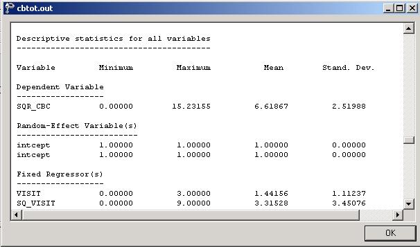
146 146

147 Fixed effects results The output describing the estimated fixed effects after convergence is shown next. The estimates are shown in the column with heading Estimate, and correspond to the coefficients 0, 1,, 3 in the model specification. From the z-values and associated exceedance probabilities, we see that the coefficients associated with both the time of measurement (VISIT) and squared value of the time of measurement (SQ_VISIT) are highly significant. The significance of the estimate associated with SQ_VISIT supports the tentative conclusion made during the exploratory analysis that the relationship between score and visit number cannot adequately be described by a linear relationship. While the average CBC score is expected to decrease with units between two successive visits, a smaller increase in score of is associated with the squared value of the time of measurement. Random effects results The output for the random part of the model follows, and is shown in the image below. There is significant variation in the average estimated total health expenditure at all levels, with the most variation over the patients (level-2), and the least variation over therapists (level-3). 147

148 Interpreting the results Estimated outcomes for different groups A typical patient at the start of the study is expected to have a transformed CBC score of SQR_CBC ij0 0 1 VISITij 2 SQ_VISIT 0 ij (0) (0 ) , that is, the estimated intercept. Similar equations for expected transformed scores at subsequent measurements (visits) are obtained in the same way: 2 ij1 VISIT 1: SQR_CBC (1) (1 )

149 2 2 VISIT 2 : SQR_CBCij (2) (2 ) ij3 VISIT 3: SQR_CBC (3) (3 ) The effect of the positive estimate for SQ_VISIT in slowing down the expected decrease in CBC scores over successive measurement occasions is clear from the equations above: without this estimate, the expected CBC scores at visits 1, 2, and 3 would have been , , and respectively. In terms of the actual rather than the square root of the CBC scores, the expected scores at the 4 measurement occasions under the current model are , , , and respectively. Model-based graphs Using the Plot Equations for: SQR_CBC dialog box that appears when the File, Model-based Graphs, Equations option is selected, we can graphically depict the trend in expected average squared score for the predictors VISIT and SQ_VISIT. The dialog box below shows the selection of the predictor VISIT, and in the graph requested, SQ_VISIT will be fixed at a value of

150 The graph below shows the result obtained when the Plot button is clicked after completion of the Plot Equations for: SQR_CBC dialog box as shown above. A similar plot for the predictor SQ_VISIT is given directly after. Note that, in the second graph, the increase in expected score seems larger than implied by the estimate of This is due in part to the difference in the ranges of the two predictors, as reflected in the tick marks on the X-axes of the graphs. 150

151 Figure XXX.24: Plot of SQR_CBC vs. VISIT Figure XXX.25: Plot of SQR_CBC vs. SQ_VISIT 151

152 Fit statistics and ICC From the output for the random part of the model it is clear that there is significant variation in the average estimated total health expenditure at all levels, with the most variation over the patients (level-2), and the least variation over therapists (level-3). An estimate of the percentage of variation in the outcome at a patient level, for example, is obtained as % 51.32% indicating that 51.32% of the total variance in scores is at the patient level. In contrast, % 9.69% is at the therapist level, with the remainder over measurements nested within patients Fitting a random intercept model with 3 predictors and interaction term to the data The model From the exploratory analysis, we are aware of a possibly nonlinear relationship between the transformed outcome variable SQR_CBC and the visit number, as represented by the variables VISIT and SQ_VISIT. Differences in the distributions of the transformed scores of the two gender groups also lead us to suspect that the outcome may depend to some extent on the gender of the patient. The possibility of an interaction between the time elapsed since the start of the study, as represented by VISIT and SQ_VISIT, and the gender of a patient cannot be ruled out. 152

153 The model considered in this section uses the participant's gender, visit number, squared value of the visit number, and the interaction between visit number and gender (represented by the variable GVISIT in the data spreadsheet) to predict the square root of the total score on the Child Behavior Checklist. This second order growth curve with gender and the interaction term as covariates can be expressed as follows: SQR_CBC GENF VISIT SQ_VISIT GENF *VISIT ijk 0 1 ij 2 ijk 3 ijk 4 ij ijk v v e i0 ij0 ijk As before, 0 denotes the average expected total score, 1, 2,, 4 indicate the estimated coefficients associated with the fixed part of the model, and v i0, v ij0 and e ijk represent the random part of the model Setting up the analysis The SuperMix spreadsheet cbtot.ss3 and the model specification file cbtot.mum discussed in the previous example are used a point of departure. With the model specification file open, click on the Variables tab of the Model Setup window. Add the predictors GENF and GVISIT to the model by checking the boxes next to these variables in the E column, as shown below. 153

154 Save the modified model specification file, then select the Run option from the Analysis menu to perform the analysis Discussion of results Fixed effects results The maximum likelihood estimates of the coefficients in the fixed part of the model are shown below. The statistical significance of all the effects confirm our suspicion that the CBC scores measured over time not only depend on the time of measurement and the squared value thereof, but also on the gender of the patient. A significant interaction between gender and the time of measurement is also observed. Recall that for male patients GENF was coded 0, and for females GENF was assigned a value of 1. The positive estimate of for the effect of gender indicates that males tended to have a lower score on average than females: the expected average male score is units lower on the transformed CBC scores than for females. This effect is offset by the negative estimate of the interaction effect. For males, the interaction term GVISIT assumes the value 0, but for females GVISIT is equal to 0, 1, 2, and 3 respectively at the 4 measurement occasions. The transformed score of a female patient is thus expected to be units lower at 154

155 the second visit than the score of a male patient, or a female patient at the beginning of the study. Random effects results The output for the random part of the model is given next. 155

156 As before, most variation in scores is found at a patient level, and the least variation at the therapist level. The estimated percentages of variation in outcome at patient and therapist level are and % 51.39% % 9.65% respectively. When compared to the similar percentages for the growth curve model, changes observed are negligible. The addition of the variables GENF and GVISIT did not contribute significantly to the explanation of remaining variation in the outcome at the various levels of the model Interpretation of the results Estimated outcomes for different groups For a typical patient, the expected CBC score can be calculated as SQR_CBC GENF VISIT SQ_VISIT GVISIT ijk 0 1 ij 2 ijk 3 ijk 4 ijk GENF VISIT SQ_VISIT GVISIT. ijk ij ijk ijk For male patients GENF = 0, and thus the formula used to predict their CBC scores reduces to 156

157 SQR_CBC (0) VISIT ijk SQ_VISIT (0) ijk VISIT SQ_VISIT. For female patients GENF = 1, and thus the formula used to predict their CBC scores can be expressed as ijk ijk ijk SQR_CBC (1) VISIT ijk SQ_VISIT GVISIT ijk VISIT SQ_VISIT GVISIT. ijk ijk ijk ijk ijk Table XXX.9 below shows the expected square roots of CBC scores for the various groups formed by the gender groups and interaction term at all measurement occasions. In Table XXX.10, the same expected scores are given in the scale of the original total score on the Child Behavioral Checklist. The initial impression, based on the positive coefficient of GENF, that females had higher expected CBC scores than males, seems to hold at the onset of the study. However, these tables show that, after the effects of the other variables are also taken into account, females are likely to have a slightly lower score than males at the end of the study period. Table XXX.9: Expected square root of CBC scores Gender Visit Male Female

158 Table XXX.10: Expected CBC scores in original scale Gender Visit Male Female The results in these tables can also be depicted graphically using the File, Modelbased Graphs menu. This menu offers three options, namely equation modeling, residual plots and confidence intervals for random effects. Equation modeling To plot the trends in CBC scores for gender groups over successive visits, make sure the Model Setup window is activated by clicking on it before select the Equations option from the File, Model-based Graphs menu. 158

159 This activates the Plot Equations for: SQR_CBC dialog box. Select VISIT as the predictor, and request marking by gender as shown in the image below. Note that, by default, remaining predictors are fixed at 0. Click Plot to display the graphing window. Figure XXX.26: Plot of SQR_CBC vs. VISIT for gender groups By default, graphs using a two-category marking variable such as GENF will be displayed using blue and green to indicate the categories. To make the distinction between the groups of interest more clear, and create a graph that can be included in a report or paper to be printed in black and white, the plotting symbols can be changed. Here, we opt to change the line for female patients to a black, dotted line. Double-click on the line for this group in the legend box shown at the top right of the graph to activate the Plot Parameters dialog box. Next, click the Line Attributes button to load the Line Parameters dialog box. Change the line style to dotted using the Style drop-down list box, and select black from the Color drop-down list box. Click OK on both the Line Parameters and Plot Parameters dialog boxes to obtain the final graph shown below. 159

160 Figure XXX.27: Modified plot of SQR_CBC vs. VISIT for gender groups The predicted decrease in CBC score echoes the results of the maximum likelihood estimation of the fixed effects, where a negative coefficient of was reported for the predictor VISIT. While the predicted intercept for males at the beginning of the study is approximately 7.5 as indicated in the graph at the top-left of the graphing window, the predicted intercept for the same group has decreased to approximately 4.75 by the final visit. This is lower than reported in Table XXX.10, where calculations showed an expected CBC score of 6.00 for males by the final 160

161 visit. The reason for this difference can be found in the formula used to produce the graph: recall that all remaining predictors were fixed to a value of 0. Whereas the result for males at the final visit shown in Table XXX.10 was based on the calculation SQR_CBC (0) VISIT ijk SQ_VISIT (0) ijk VISIT SQ_VISIT, ijk ijk ijk the line shown for this group in the graph above is based on the formula SQR_CBC (0) ijk VISIT ijk. As a result, the predicted outcome shown in the graph for males at the end of the study will be ( )( 9) units lower than reported in Table XXX.10. This difference underlines the fact that care should be taken when selecting the treatment for remaining predictors in the model. In this case, both SQ_VISIT and GVISIT can assume the value of 0, and thus using the remaining predictors fixed at zero option is permissible. In cases where predictors cannot assume a value of zero, the better choice would be to fix remaining predictors at their mean values instead when completing the Plot Equations for: dialog box. Confidence intervals for random coefficients The Confidence Intervals option on the File, Model-based Graphs menu provides the option to display confidence intervals for the empirical Bayes estimates of the random effects specified in a given model. This option is now used to examine the confidence intervals of the random intercepts for the therapists, who represent the highest level of the hierarchy in the current example. Select the Confidence Intervals option on the File, Model-based Graphs menu to activate the 95% Conf. Intervals for EB estimates dialog box. A simple graph of the 161

162 confidence intervals for the empirical Bayes estimates of the intercepts at the therapist level is obtained by selecting THERAPIST Intcept in the Predictor column before clicking Plot. Note that it is also possible to select both a grouping and marking variable to be used in the graph. The graph obtained, as seen below, shows that, in general, the range of the confidence intervals for the level-3 empirical Bayes estimates of the intercepts is ( 2; 2). The deviations from the estimated population intercept over therapists are also apparent. Each confidence interval is obtained using Empirical Bayes residuals var Empirical Bayes residuals. 162

163 Figure XXX.28: 95% confidence intervals for level-3 units Fit statistics Recall that for the growth curve model the following indices were obtained: o Log Likelihood: o -2 Log Likelihood (Deviance): o Akaike's Information Criterion: o Schwarz's Bayesian Criterion: o Number of free parameters: 6 2 When the deviances of the two models are compared, a -statistic of = with 8 6 = 2 degrees of freedom is obtained. This indicates that the current model fits the data better than the growth curve model. The AIC decreased from to , and also favors the use of the current model. The SBC, however, increased slightly, from to , and thus favors the growth curve model previously fitted as the more parsimonious. Note, however, that the changes in all three criteria are rather small. 163

164 Residuals Residual plots The Residuals option on the File, Model-based Graphs menu is used to examine the residuals obtained for a fitted model. It is useful for examining the fit of the model, and also as a check for possible distributional assumption violations. As residuals are defined as the difference between the observed and predicted outcomes, trends in residuals, for example over the course of a study in a longitudinal data set, may indicate that an important predictor was not included in the model fitted to the data. Select the Residuals option on the File, Model-based Graphs menu to activate the Plot of Residuals dialog box. To simultaneously check for any differences in residuals for the gender groups, select GENF as marking variable. Opt to create an unstandardized plot of the residuals by selecting the Unstandardized Plot option rather than the default Standardized Plot option. Click Plot. The graph below shows the residuals for the gender groups in the default colors of blue and green. To make the distinction between the groups more clear, click on the plotting symbol for the female group in the legend box. 164

165 Figure XXX.29: Level-1 residual plot by gender group The Plot Parameters dialog box appears. Change the Shape of the symbol to "Up Triangle," adjust the Size to 3 and change the display Color to black as shown below. Click OK when done. 165

166 Click on the symbol for the male group next, and change the parameters for this group to those shown in the dialog box below. Click OK to return to the graphing window. The final plot is shown below. The residuals are clustered reasonably symmetrically around the 0 tick mark on the Y-axis, and no gender pattern can be discerned for the larger residuals. A single residual, for a male respondent, has a value larger than 10. This potential outlier can be identified using the Data option on the Plot Parameters dialog box (see above). 166

167 Figure XXX.30: Modified level-1 residual plot by gender group Fitting a random intercepts and slopes model The model The graphs obtained during the exploratory analysis of the CBC data showed that the change in total CBC score over the course of the study differed from patient to patient. Because of this, the models fitted in Sections XXX.2 and XXX.3 allowed for the intercepts to vary randomly at both patient and therapist level. In effect, we assumed that each patient may have a different starting point. These models indicated a statistically significant relationship between the observed CBC score and the measurement occasion. To test whether there is significant variation in the way individual patients' scores change over the study period, a model in which both intercepts and slopes of the predictor VISIT are allowed to vary randomly can be used. The model can be formulated as SQR_CBC GENF VISIT SQ_VISIT GENF *VISIT ijk 0 1 ij 2 ijk 3 ijk 4 ij ijk ( v v *VISIT ) ( v v VISIT ) e i0 i1 ijk ij0 ij1 ijk ijk 167

168 At level 2, two random coefficients are now included: v ij0 represents the random intercept and v ij1 the random coefficient for the slope of the predictor VISIT. The random coefficients v i0 and v i1 serve the same purpose at level 3 (the therapist level) of the model Setting up the analysis Again, we use the SuperMix spreadsheet cbtot.ss3 and the model specification file cbtot.mum discussed in the previous example as the starting point. With the model specification file open, click on the Variables tab of the Model Setup window. Add random coefficients for the predictor VISIT to levels 2 and 3 of the model by checking the boxes next to these variables in the 2 and 3 column, as shown below. Save the changes to the model specification file, using the File, Save option to overwrite the previous specification file or the File, Save as option to assign a new filename. Click Run on the Analysis menu to perform the analysis. 168

169 Discussion of results Partial output is given below. We focus on those parts of the output that differ from the output obtained for the previous analysis, and conclude with a discussion of the additional output files containing the empirical Bayes residuals. Fixed effects results The inclusion of random VISIT slopes at levels 2 and 3 of the hierarchy has very little impact the estimated fixed coefficients. Results for the fixed part are shown below. Random effects results Turning to the estimated coefficients in the random part of the model, we note a change in the between measurement (level-1) variation, which has decreased from to This illustrates that the addition of a random coefficient at any level of a model can affect the random effect(s) at another level. 169

170 At levels 2 and 3 we find evidence of significant variation in the VISIT slopes. While not of the same magnitude as the intercept variation, it is clear that it is more realistic to allow the slopes to vary from patient to patient, and from therapist to therapist, than to assume that the VISIT slope can be described adequately by a common fixed effect as was done in the previous model Interpreting the results Fit statistics and ICC Model fit When the measures of fit are compared to those of the random-intercepts-only model, it becomes clear that the current model fits the data better. Recall that for the random intercepts model the following fit measures were obtained: o Log likelihood: o -2 log Likelihood (Deviance): o Akaike s Information Criterion: o Schwarz s Bayesian Criterion: o Number of free parameters: 8 170