Chapter 5 Roots of Equations: Bracketing Models. Gab-Byung Chae

Transcription

1 Chapter 5 Roots of Equations: Bracketing Models Gab-Byung Chae

2 2 Chapter Objectives Studying Bracketing Methods Understanding what roots problems are and where they occur in engineering and science. Knowing how to determine a root graphically. Understanding the incremental search method and its shortcoming. Knowing how to solve a roots problem with the bisection method. Knowing how to estimate the error of bisection Understanding false position and how it differs from bisection. You ve got a problem A bungee jumper s chances of sustaining a significant vertebrae injury increase significantly if the free-fall velocity exceeds 36m/s after 4 s of free fall. ( ) gm gcd v(t) = tanh m t Can you solve this equation when c d = 0.25kg/m for the mass? c d An alternative way of looking at the problem involves subtracting v(t) from both sides to give a new function: gm f(m) = c d (1) ( ) gcd tanh m t v(t) (2) Now we can see that the answer to the problem is the value of m that makes the function equal to zero. Hence we call this a roots problem. 5.1 INTRODUCTION AND BACKGROUND What Are Roots? Quadratic formula x = b ± b 2 4ac 2a (3)

3 3 to solve f(x) = ax 2 + bx + c = 0 (4) Roots of Equations and Engineering Practice Eq.(1) can be used to predict the jumper s velocity. Such computations can be performed directly because v is expressed explicitly as a function of the model parameters. Suppose we had to determine the mass for a jumper with a given drag coefficient to attain a prescribed velocity in a set time period. Eq.(1) cannot be solved explicitly for mass. In such cases, m is said to be implicit. The solution to the implicit equations is provided by numerical methods for roots of equations as in Eq.(2) 5.2 GRAPHICAL METHODS Example 0.1 The Graphical Approach Use the graphical approach to determine the mass of the bungee jumper with a drag coefficient of 0.25kg/m to have a velocity of 36m/s after 4 s of free fall. The acceleration of gravity is 9.81m/s 2. Solution >> cd = 0.25; g = 9.81; v = 36; t = 4; >> mp = linspace(50,200);

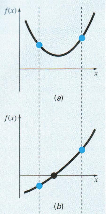
4 4 >> fp = sqrt(g*mp/cd).*tanh(sqrt(g*cd./mp)*t)-v; >> plot(mp,fp),grid The function crosses the m axis between 140 and 150kg. The validity of the graphical estimate can be checked by substituting it into Eq.(2) to yield >> sqrt(g*145/cd).*tanh(sqrt(g*cd./145)*t) ans = which is close to the desired fall velocity of 36m/s. Graphical methods can be utilized to obtain rough estimates of roots. These estimates can be employed as starting guesses for numerical methods discussed in this chapter. Figure 5.1 shows a number of ways in which roots can occur (or absent ) in an interval. 5.3 BRACKETING METHODS AND INITIAL GUESSES Trial and Error : You should repeatedly make guesses until the function is sufficiently close to zero.

5 5

6 6 The two major classes of methods available are distinguished by the type of initial guess. Bracketing methods. As the name implies, these are based on two initial guesses that bracket the root-that is, are on either side of the root. Open methods. These methods can involve one or more initial guesses, but there is no need for them to bracket the root. The bracketing methods work but converge slowly. The open methods do not always work, but when they do they usually converge quicker. In both cases, initial guesses are required. How to make a good initial guess? The following section describes one such approach, the incremental search Incremental Search You observed that f(x) changed sign on opposite sides of the root. In general, f(x) is real and continuous in the interval from x l to x u and f(x l ) and f(x u ) have opposite signs, that is, f(x l )f(x u ) < 0 then there is at least one real root between x l and x u. Incremental search methods capitalize on this observation by locating an interval where the function changes sign. An M-file can be developed that implements an incremental search to locate the roots of a function func within the range from xmin to xmax. ns : the number of intervals within the range. (default is 50) function xb = incsearch(func, xmin, xmax,ns ) % incsearch(func, xmin, xmax,ns ): % find brackets of x that contain sign changes of % a function on an interval % input: % func = name of function

7 7 % xmin, xmax = endpoints of interval % ns = (optional) number of subintervals along x % used to search for brackets %output: % xb(k,1) is the lower bound of the kth sign change % xb(k,2) is the upper bound of the kth sign change % If no brackets found, xb = []. if nargin < 4, ns = 50 ; end % if ns blank set to 50 % Incremental search x = linspace(xmin,xmax,ns); f = feval(func,x); nb = 0; xb=[ ]; %xb is null unless sign change detected for k =1 : length(x) -1 if sign(f(k)) ~= sign(f(k+1)) % check for sign change nb = nb + 1; xb(nb,1) = x(k); xb(nb,2) = x(k+1); end end if isempty(xb) % display that no brackets were found disp( no brackets found ) disp( check interval or increase ns ) else disp( number of brackets: ) % display number of brackets disp(nb) end Example 0.2 Use the M-file incsearch to identify brackets within the inter-

8 8 val [3, 6] for the function: f(x) = sin(10x) + cos(3x) Solution >> incsearch( inline( sin(10*x) +cos(3*x) ),3,6) number of brackets: 5 ans = >> incsearch( inline( sin(10*x) +cos(3*x) ),3,6,100) number of brackets:

9 9 9 ans = BISECTION The bisection method is a variation of the incremental search method in which the interval in the ith iteration is always divided in half in (i + 1)th iteration.

10 10 Example 0.3 The Bisection Method Use bisection to solve the same problem approached graphically in Example 5.1 Solution From the graphical solution in Example 5.1, we can see that the function changes sign between values of 50 and 200(Let s assume). Therefore, the initial estimate of the root x r lies at the midpoint of the interval x r = = 125 Next we compute the product of the function value at the lower bound and at the midpoint : f(50)f(125) = 4.579( 0.409) = > 0 which means that the root must be located in the upper interval between 125 and 200. The new interval extends from x l = 125 to x u = 200. x r = = And f(125)f(162.5) = 0.409(0.359) = < 0

11 11 Therefore, the root is now in the lower interval between 125 and The upper bound is redefined as and the root estimate for the third iteration is calculated as x r = = which represent a percent relative error of ε t = % = 0.709% The method can be repeated until the result is accurate enough to satisfy your needs. But how? We do not know the true value!! So we use an approximate percent relative error as in Eq.(4.5) ε a = where x new r previous iteration. Example 0.4 x new r x old r x new r is the root for the present iteration and x old r Error Estimate for Bisection 100% (5) is the root from the Continue Example 5.3 until the approximate error falls below a stopping criterion of ε s = 0.5%. Use Eq.(5) to compute the errors. Solution The results for the first two iterations for Example 5.3 were 125 and By Eq.(5) ε a = % = 23.08% After eight iterations ε a finally falls below ε s = 0.5%, and the computation can be terminated. The Fig.5.6 exhibits the extremely attractive characteristic that ε a is always greater than ε t (generally this is true for bisection, Why?). Thus, when ε a falls

12 12 below ε s, the computation could be terminated with confidence that the root is known to be at least as accurate as the prespecified acceptable level. This is the one benefit of the bisection. Another benefit of the bisection : The number of iterations required to attain an absolute error can be computed a priori MATLAB M-file : bisection function root = bisection(func, xl, xu, es, maxit ) % bisection(func, xl, xu, es, maxit ): % use bisection method to find the root of a function % input: % func = name of function % xl, xu = lower and upper guesses % es = (optional) stopping criterion (%) % maxit = (optional) maximum allowable iterations %output: % rooot = real root if func(xl)*func(xu) >0 error( no bracket ) %if guesses do not bracket a sign %change, display an error message

13 13 end return %and terminate %if necessary, assign default values if nargin < 5, maxit = 50 ; end %if maxit blank set to 50 if nargin < 4, es = 0.001; end %if es blank set to % bisection iter =0; xr = xl; while (1) xrold = xr; xr = (xl + xu)/2; iter = iter + 1 ; if xr~= 0, ea = abs((xr - xrold)/xr)* 100; end test = func(xl)*func(xr); if test < 0 xu = xr ; elseif test > 0 xl = xr; else ea = 0 ; end if ea <= es iter >= maxit, break, end end root = xr; 5.5 FALSE POSITION False position(also called the linear interpolation method) is another wellknown bracketing method. It uses a different strategy to come up with its new root estimate.

14 14 It locates the root by joining f(x l ) and f(x u ) with a straight line(see Figure). The intersection of this line with the x axis represents an improved estimate of the root. Using similar triangles, we have f(x l ) : f(x u ) = (x r x l ) : (x u x r ) or Therefore x r = f(x l)x u f(x u )x l f(x l ) f(x u ) x r = x u f(x u)(x l x u ) f(x l ) f(x u ) This is the false-position formula. The value of x r computed with Eq.(6) then replaces whichever of the two initial guesses, x l or x u, yields a function value with the same sign as f(x r ). (HOMEWORK : implement false-position method using MATLAB) Example 0.5 The False-Position Method Use false position to solve the same problem approached graphically and with bisection in Example 5.1 and 5.3. Solution (6)

15 15 With initial guesses x l = 50 and x u = 200 First iteration : x r = 200 which has a true relative error of 23.5%. Second iteration : x l = 50 f(x l ) = x u = 200 f(x u ) = (50 200) = f(x l )f(x r ) = Therefore, the root lies in the first subinterval, and x r becomes the upper limit for the next iteration, x u = x r = x l = 50 f(x l ) = x u = f(x u ) = ( ) = which has a true and approximate relative errors of 13.76% and 8.56%, respectively. False position method often performs better than bisection, but not always. Example 0.6 A Case Where Bisection Is Preferable to False Position f(x) = x 10 1 between x = 0 and 1.3. Bisection : False position: See Figure 5.9

16 16