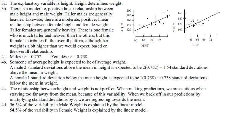
appstats8.notebook October 11, 2016

Transcription

1 Chapter 8 Linear Regression Objective: Students will construct and analyze a linear model for a given set of data.

2 Fat Versus Protein: An Example pg 168 The following is a scatterplot of total fat versus protein for 30 items on the Burger King menu: Correlation says There seems to be a linear association between these two variables, but it doesn t tell what that association is. The Linear Model pg 169 We can say more about the linear relationship between two quantitative variables with a model. A model simplifies reality to help us understand underlying patterns and relationships.

3 Linear Regression Now that we know how to observe thedirection and strength of a linear relationship, we can model the relationship. Just as we used a Normal Model to approximate distributions of data that were unimodal and symmetric, We can use a linear model to make approximate predictions about a data set showing a linear relationship. The Linear Model (cont.) pg 169 The linear model is just an equation of a straight line through the data. The points in the scatterplot don t all line up, but a straight line can summarize the general pattern. The linear model can help us understand how the values are associated.

4 Correlation and the Line pg 170 Moving one standard deviation away from the mean in x moves us r standard deviations away from the mean in y. This relationship is shown in a scatterplot of z scores for fat and protein:

5 Correlation and the Line (cont.) pg 170 Put generally, moving any number of standard deviations away from the mean in x moves us r times that number of standard deviations away from the mean in y. How Big Can Predicted Values Get? pg 172 r cannot be bigger than 1 (in absolute value), so each predicted y tends to be closer to its mean (in standard deviations) than its corresponding x was. This property of the linear model is called regression to the mean; the line is called the regression line.

6 The Least Squares Line pg 174 We write our model as This model says that our predictions from our model follow a straight line. If the model is a good one, the data values will scatter closely around it. The Least Squares Line (cont.) pg 174 In our model, we also have an intercept (b 0 ). The intercept is built from the means and the slope: Our intercept is always in units of y.

7 The Least Squares Line (cont.) pg 174 In our model, we have a slope (b 1 ): The slope is built from the correlation and the standard deviations: Our slope is always in units of y per unit of x. The Least Squares Line (cont.) Since regression and correlation are closely related, we need to check the same conditions for regressions as we did for correlations: Quantitative Variables Condition Straight Enough Condition Outlier Condition pg 176 see step by step

8 Fat Versus Protein: An Example pg 175 The regression line for the Burger King data fits the data well: The equation is The predicted fat content for a BK Broiler chicken sandwich is (30) = 35.9 grams of fat. Assumptions and Conditions Quantitative Variables Condition: pg 176 Regression can only be done on two quantitative variables, so make sure to check this condition. Straight Enough Condition: The linear model assumes that the relationship between the variables is linear. A scatterplot will let you check that the assumption is reasonable.

9 Assumptions and Conditions (cont.) Outlier Condition: Watch out for outliers. Outlying points can dramatically change a regression model. Outliers can even change the sign of the slope, misleading us about the underlying relationship between the variables. Assumptions and Conditions (cont.) pg It s a good idea to check linearity again after computing the regression when we can examine the residuals. 2.You should also check for outliers, which could change the regression. 3.If the data seem to clump or cluster in the scatterplot, that could be a sign of trouble worth looking into further.

10 Assumptions and Conditions (cont.) pg 176 see step by step go over If the scatterplot is not straight enough, stop here. You can t use a linear model for any two variables, even if they are related. They must have a linear association or the model won t mean a thing. Some nonlinear relationships can be saved by re expressing the data to make the scatterplot more linear. Example 1

11 Example 1 Objectives: Students will be able to interpret the slope and y intercept of a linear model in context of the data. Students will be able to informally assess the fit of a function by plotting and analyzing residuals.

12 Residuals pg 169 The model won t be perfect, regardless of the line we draw. Some points will be above the line and some will be below. The estimate made from a model is the predicted value (denoted as ). Residuals Revisited pg 178 The linear model assumes that the relationship between the two variables is a perfect straight line. The residuals are the part of the data that hasn t been modeled. Data = Model + Residual or (equivalently) Residual = Data Model Or, in symbols,

13 Residuals (cont.) pg 169 The difference between the observed value and its associated predicted value is called the residual. To find the residuals, we always subtract the predicted value from the observed one: Let's go back to the example unit test 1 and semester test Residual Plots predicted A residual is the difference between the observed y value and the y value for a given x value. residual = y yˆ Sum of the least Square Residuals The (SSR) is used to determine the Least Squares Regression Line for a given set of data.

14 Best Fit Means Least Squares pg 170 Some residuals are positive, others are negative, and, on average, they cancel each other out. So, we can t assess how well the line fits by adding up all the residuals. Similar to what we did with deviations, we square the residuals and add the squares. The smaller the sum, the better the fit. The line of best fit is the line for which the sum of the squared residuals is smallest. Residuals (cont.) pg 169 A negative residual means the predicted value s too big (an overestimate). A positive residual means the predicted value s too small (an underestimate).

15 Residuals Revisited (cont.) pg 178 Residuals help us to see whether the model makes sense. When a regression model is appropriate, nothing interesting should be left behind. After we fit a regression model, we usually plot the residuals in the hope of finding nothing. Residuals Revisited (cont.) pg 178 The residuals for the BK menu regression look appropriately boring:

16 closure A is a scatterplot which graphs the residuals on the axis and the values of the explanatory variable on the axis for each data point,( ) The residual plot gives a visual representation of the amount of error in the model. The closer the residuals are to, the smaller the error and the more accurate the model. The LSRL is a good model if the residual plot shows random relatively close to the horizontal axis (zero). The horizontal axis represents the. Points in the residual plot that lie directly on the horizontal axis lie directly on the. Points in the residual plot that lie above the horizontal axis lie the LSRL. Therefore, the model gives an underestimate at that point. Therefore residuals represent underestimates. Points in the residual plot that lie below the horizontal axis, lie the LSRL. Therefore the model gives an overestimate at that point. Therefore residuals represent overestimates. The LSRL is not a good model if the residual plot shows.

17 Objectives: Students will be able calculate the coefficient of determination and interpret its value for evaluating the regression line. R 2 The Variation Accounted For pg 179 The variation in the residuals is the key to assessing how well the model fits. In the BK menu items example, total fat has a standard deviation of 16.4 grams. The standard deviation of the residuals is 9.2 grams.

18 R 2 The Variation Accounted For (cont.) pg 179 If the correlation were 1.0 and the model predicted the fat values perfectly, the residuals would all be zero and have no variation. As it is, the correlation is 0.83 not perfection. However, we did see that the model residuals had less variation than total fat alone. We can determine how much of the variation is accounted for by the model and how much is left in the residuals. Review The residuals also reveal how well the model works. If a plot of the residuals against predicted values shows a pattern, we should re examine the data to see why. The standard deviation of the residuals quantifies the amount of scatter around the line.

19 R 2 The Variation Accounted For (cont.) pg 179 The squared correlation, r 2, gives the fraction of the data s variance accounted for by the model. Thus, 1 r 2 is the fraction of the original variance left in the residuals. For the BK model, r 2 = = 0.69, so 31% of the variability in total fat has been left in the residuals. R 2 The Variation Accounted For (cont.) pg 179 All regression analyses include this statistic, although by tradition, it is written R 2 (pronounced R squared ). An R 2 of 0 means that none of the variance in the data is in the model; all of it is still in the residuals. When interpreting a regression model you need to Tell what R 2 means. In the BK example, 69% of the variation in total fat is accounted for by the model.

20 How Big Should R 2 Be? pg 180 R 2 is always between 0% and 100%. What makes a good R 2 value depends on the kind of data you are analyzing and on what you want to do with it. The standard deviation of the residuals can give us more information about the usefulness of the regression by telling us how much scatter there is around the line. Reporting R 2 pg see TI Tips see step by step Along with the slope and intercept for a regression, you should always report R 2 so that readers can judge for themselves how successful the regression is at fitting the data. Statistics is about variation, and R 2 measures the success of the regression model in terms of the fraction of the variation of y accounted for by the regression.

21 Coefficient of Determination The coefficient of determination, also called R 2, is the square of the. The R 2 valuetells how much of the variation in the response variable is accounted for by the linear regression model. 100 correlation For example, if R 2 = 1, then % of the variability in the response variable is accounted for by thelinear model. In other words, the relationship between the two variables is perfectly linear. 95 If R 2 = 0.95,we can conclude that % of the variability in the response variable is accounted for by the linear relationship with the explanatory variable. Example 2. A study of class attendance and grades earned among first year students at a state university showed that in general students who attended a higher percent of their classes earned higher grades. Class attendance explained 16% of the variation in grades among the students. What is the numerical correlation between percent of classes attended and grades earned? Closure

22 Reality Check: Is the Regression Reasonable? pg 184 Statistics don t come out of nowhere. They are based on data. The results of a statistical analysis should reinforce your common sense, not fly in its face. If the results are surprising, then either you ve learned something new about the world or your analysis is wrong. When you perform a regression, think about the coefficients and ask yourself whether they make sense.

23 What Can Go Wrong? pg 185 Don t fit a straight line to a nonlinear relationship. Beware extraordinary points (y values that stand off from the linear pattern or extreme x values). Don t extrapolate beyond the data the linear model may no longer hold outside of the range of the data. Don t infer that x causes y just because there is a good linear model for their relationship association is not causation. Don t choose a model based on R 2 alone. What have we learned? pg 186 When the relationship between two quantitative variables is fairly straight, a linear model can help summarize that relationship. The regression line doesn t pass through all the points, but it is the best compromise in the sense that it has the smallest sum of squared residuals.

24 What have we learned? (cont.) pg 186 The correlation tells us several things about the regression: 1)The slope of the line is based on the correlation, adjusted for the units of x and y. 2)For each SD in x that we are away from the x mean, we expect to be r SDs in y away from the y mean. 3)Since r is always between 1 and +1, each predicted y is fewer SDs away from its mean than the corresponding x was (regression to the mean). 4)R 2 gives us the fraction of the response accounted for by the regression model. What have we learned? pg 186 The residuals also reveal how well the model works. If a plot of the residuals against predicted values shows a pattern, we should re examine the data to see why. The standard deviation of the residuals quantifies the amount of scatter around the line.

25

26

27 1. Below are heights and weights data for male and female AP Stat students. Create TI lists MHT, MWT, FHT, FWT, and enter the data. You will need to keep these data for several days. Remember, to create a list: 1 put the cursor atop the names L1,L2,..., then 2 space to the right, and 3 type the new name in the blank space. You can then access these names via the LIST NAMES menu. 2. Is it reasonable to assume these data are drawn from populations that are normally distributed? Check summary statistics and histograms for each variable. 3. a Make a scatterplot for each gender STAT PLOT, first plot type. Which is the explanatory variable? b Describe the relationship form, strength, direction, outliers, etc. for each gender. 4. a Calculate and interpret r for each gender. b What would you predict about the weight of... someone of average height?... a male 2 standard deviations above average in height.... a female 1 standard deviation below average in height? c Explain how this illustrates the concept of regression toward the mean. d Calculate the coefficients of determination, r2, and interpret each in the context of this relationship. 5. a Write an equation of the least squares line of best fit for each gender. b Check the residuals plots. Do you think that a line is a good model? Explain. c Explain what the slope of each line means in the context of this relationship. d Predict weights for : a 60 male; a 60 female; a 70 male; a 70 female e Predict the weight of a 7 2 male; of a 20 newborn baby girl. Comment on these results.

28

29