CS70: Jean Walrand: Lecture 19.

Transcription

1 CS70: Jean Walrand: Lecture 19. Random Variables: Expectation 1. Random Variables: Brief Review 2. Expectation 3. Important Distributions

2 Random Variables: Definitions Definition A random variable, X, for a random experiment with sample space Ω is a function X : Ω R. Thus, X( ) assigns a real number X(ω) to each ω Ω. Definitions (a) For a R, one defines (b) For A R, one defines X 1 (a) := {ω Ω X(ω) = a}. X 1 (A) := {ω Ω X(ω) A}. (c) The probability that X = a is defined as Pr[X = a] = Pr[X 1 (a)]. (d) The probability that X A is defined as Pr[X A] = Pr[X 1 (A)]. (e) The distribution of a random variable X, is {(a,pr[x = a]) : a A }, where A is the range of X. That is, A = {X(ω),ω Ω}.

3 Random Variables: Definitions Definition Let X,Y,Z be random variables on Ω and g : R 3 R a function. Then g(x,y,z ) is the random variable that assigns the value g(x(ω),y (ω),z (ω)) to ω. Thus, if V = g(x,y,z ), then V (ω) := g(x(ω),y (ω),z (ω)). Examples: X k (X a) 2 a + bx + cx 2 + (Y Z ) 2 (X Y ) 2 X cos(2πy + Z ).

4 Expectation - Definition Definition: The expected value (or mean, or expectation) of a random variable X is Theorem: E[X] = a Pr[X = a]. a E[X] = X(ω) Pr[ω]. ω

5 An Example Flip a fair coin three times. Ω = {HHH,HHT,HTH,THH,HTT,THT,TTH,TTT }. X = number of H s: {3,2,2,2,1,1,1,0}. Thus, Also, X(ω)Pr[ω] = { } 1 ω 8. a Pr[X = a] = 3 1 a

6 Win or Lose. Expected winnings for heads/tails games, with 3 flips? Recall the definition of the random variable X: {HHH,HHT,HTH,HTT,THH,THT,TTH,TTT } {3,1,1, 1,1, 1, 1, 3}. E[X] = = 0. Can you ever win 0? Apparently: expected value is not a common value, by any means. The expected value of X is not the value that you expect! It is the average value per experiment, if you perform the experiment many times: X X n, when n 1. n The fact that this average converges to E[X] is a theorem: the Law of Large Numbers. (See later.)

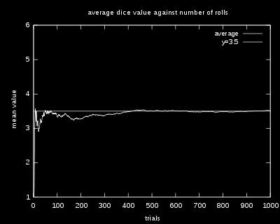
7 Law of Large Numbers An Illustration: Rolling Dice

8 Indicators Definition Let A be an event. The random variable X defined by { 1, if ω A X(ω) = 0, if ω / A is called the indicator of the event A. Note that Pr[X = 1] = Pr[A] and Pr[X = 0] = 1 Pr[A]. Hence, E[X] = 1 Pr[X = 1] + 0 Pr[X = 0] = Pr[A]. This random variable X(ω) is sometimes written as Thus, we will write X = 1 A. 1{ω A} or 1 A (ω).

9 Linearity of Expectation Theorem: Expectation is linear E[a 1 X a n X n ] = a 1 E[X 1 ] + + a n E[X n ]. Proof: E[a 1 X a n X n ] = (a 1 X a n X n )(ω)pr[ω] ω = (a 1 X 1 (ω) + + a n X n (ω))pr[ω] ω = a 1 ω X 1 (ω)pr[ω] + + a nx n (ω)pr[ω] ω = a 1 E[X 1 ] + + a n E[X n ]. Note: If we had defined Y = a 1 X a n X n has had tried to compute E[Y ] = y ypr[y = y], we would have been in trouble!

10 Using Linearity - 1: Pips (dots) on dice Roll a die n times. X m = number of pips on roll m. X = X X n = total number of pips in n rolls. E[X] = E[X X n ] = E[X 1 ] + + E[X n ], by linearity = ne[x 1 ], because the X m have the same distribution Now, E[X 1 ] = = = 7 2. Hence, E[X] = 7n 2. Note: Computing x xpr[x = x] directly is not easy!

11 Using Linearity - 2: Fixed point. Hand out assignments at random to n students. X = number of students that get their own assignment back. X = X X n where X m = 1{student m gets his/her own assignment back}. One has E[X] = E[X X n ] = E[X 1 ] + + E[X n ], by linearity = ne[x 1 ], because all the X m have the same distribution = npr[x 1 = 1], because X 1 is an indicator = n(1/n), because student 1 is equally likely to get any one of the n assignments = 1. Note that linearity holds even though the X m are not independent (whatever that means). Note: What is Pr[X = m]? Tricky...

12 Using Linearity - 3: Binomial Distribution. Flip n coins with heads probability p. X - number of heads Binomial Distibution: Pr[X = i], for each i. ( ) n Pr[X = i] = p i (1 p) n i. i E[X] = i i Pr[X = i] = i i Uh oh.... Or... a better approach: Let { 1 if ith flip is heads X i = 0 otherwise E[X i ] = 1 Pr[ heads ] + 0 Pr[ tails ] = p. Moreover X = X 1 + X n and ( ) n p i (1 p) n i. i E[X] = E[X 1 ] + E[X 2 ] + E[X n ] = n E[X i ]= np.

13 Using Linearity - 4 Assume A and B are disjoint events. Then 1 A B (ω) = 1 A (ω) + 1 B (ω). Taking expectation, we get Pr[A B] = E[1 A B ] = E[1 A + 1 B ] = E[1 A ] + E[1 B ] = Pr[A] + Pr[B]. In general, 1 A B (ω) = 1 A (ω) + 1 B (ω) 1 A B (ω). Taking expectation, we get Pr[A B] = Pr[A] + Pr[B] Pr[A B]. Observe that if Y (ω) = b for all ω, then E[Y ] = b. Thus, E[X + b] = E[X] + b.

14 Calculating E[g(X)] Let Y = g(x). Assume that we know the distribution of X. We want to calculate E[Y ]. Method 1: We calculate the distribution of Y : Pr[Y = y] = Pr[X g 1 (y)] where g 1 (x) = {x R : g(x) = y}. This is typically rather tedious! Method 2: We use the following result. Theorem: Proof: E[g(X)] = ω = x E[g(X)] = g(x)pr[x = x]. x g(x(ω))pr[ω] = x ω X 1 (x) = g(x)pr[x = x]. x ω X 1 (x) g(x)pr[ω] = x g(x) g(x(ω))pr[ω] ω X 1 (x) Pr[ω]

15 An Example Let X be uniform in { 2, 1,0,1,2,3}. Let also g(x) = X 2. Then (method 2) E[g(X)] = 3 x= 2x = { } 1 6 = Method 1 - We find the distribution of Y = X 2 : 4, w.p , w.p. 2 Y = 6 0, w.p , w.p Thus, E[Y ] = = 19 6.

16 Calculating E[g(X,Y,Z )] We have seen that E[g(X)] = x g(x)pr[x = x]. Using a similar derivation, one can show that E[g(X,Y,Z )] = g(x,y,z)pr[x = x,y = y,z = z]. x,y,z An Example. Let X,Y be as shown below: Y (0, 0), w.p. 0.1 >< (1, 0), w.p. 0.4 (X, Y )= (0, 1), w.p. 0.2 >: (1, 1), w.p X E[cos(2πX + πy )] = 0.1cos(0) + 0.4cos(2π) + 0.2cos(π) + 0.3cos(3π) = ( 1) ( 1) = 0.

17 Best Guess: Least Squares If you only know the distribution of X, it seems that E[X] is a good guess for X. The following result makes that idea precise. Theorem The value of a that minimizes E[(X a) 2 ] is a = E[X]. Proof 1: E[(X a) 2 ] = E[(X E[X] + E[X] a) 2 ] = E[(X E[X]) 2 + 2(X E[X])(E[X] a) + (E[X] a) 2 ] = E[(X E[X]) 2 ] + 2(E[X] a)e[x E[X]] + (E[X] a) 2 = E[(X E[X]) 2 ] (E[X] a) 2 E[(X E[X]) 2 ].

18 Best Guess: Least Squares If you only know the distribution of X, it seems that E[X] is a good guess for X. The following result makes that idea precise. Theorem The value of a that minimizes E[(X a) 2 ] is a = E[X]. Proof 2: Let g(a) := [(X a) 2 ] = E[X 2 2aX + a 2 ] = E[X 2 ] 2aE[X] + a 2. To find the minimizer of g(a), we set to zero d da g(a). We get 0 = d da g(a) = 2E[X] + 2a. Hence, the minimizer is a = E[X].

19 Best Guess: Least Absolute Deviation Thus E[X] minimizes E[(X a) 2 ]. It must be noted that the measure of the quality of the approximation matters. The following result illustrates that point. Theorem The value of a that minimizes E[ X a ] is the median of X. The median ν of X is any real number such that Pr[X ν] = Pr[X ν]. Proof: g(a) := E[ X a ] = x a (a x)pr[x = x] + x a (x a)pr[x = x]. Thus, if 0 < ε << 1, g(a + ε) = g(a) + εpr[x a] εpr[x a]. Hence, changing a cannot reduce g(a) only if Pr[X a] = Pr[X a].

20 Best Guess: Illustration X 2 {1, 2, 3, 11, 13} equal probabilities E[ X a ] E[(X a) 2 ] 1 10 a median E[X] mean

21 Best Guess: Another Illustration X 2 {1, 2, 11, 13} equal probabilities E[ X a ] median E[(X a) 2 ] 1 10 a E[X] mean

22 Center of Mass The expected value has a center of mass interpretation: p 1 p 2 p X p n (a n µ)=0 a 1 a 2 a 3 n, µ = X a n p n = E[X] µ n p 1 (a 1 µ) p 3 (a 3 µ) p 2 (a 2 µ)

23 Monotonicity Definition Let X,Y be two random variables on Ω. We write X Y if X(ω) Y (ω) for all ω Ω, and similarly for X Y and X a for some constant a. Facts (a) If X 0, then E[X] 0. (b) If X Y, then E[X] E[Y ]. Proof (a) If X 0, every value a of X is nonnegative. Hence, E[X] = apr[x = a] 0. a (b) X Y Y X 0 E[Y ] E[X] = E[Y X] 0. Example: B = m A m 1 B (ω) m 1 Am (ω) Pr[ m A m ] m Pr[A m ].

24 Uniform Distribution Roll a six-sided balanced die. Let X be the number of pips (dots). Then X is equally likely to take any of the values {1,2,...,6}. We say that X is uniformly distributed in {1,2,...,6}. More generally, we say that X is uniformly distributed in {1,2,...,n} if Pr[X = m] = 1/n for m = 1,2,...,n. In that case, E[X] = n m=1 n mpr[x = m] = m=1m 1 n = 1 n n(n + 1) 2 = n

25 Geometric Distribution Let s flip a coin with Pr[H] = p until we get H. For instance: ω 1 = H, or ω 2 = T H, or ω 3 = T T H, or ω n = T T T T T H. Note that Ω = {ω n,n = 1,2,...}. Let X be the number of flips until the first H. Then, X(ω n ) = n. Also, Pr[X = n] = (1 p) n 1 p, n 1.

26 Geometric Distribution Pr[X = n] = (1 p) n 1 p,n 1.

27 Geometric Distribution Note that Pr[X n ] = n=1 n=1 Pr[X = n] = (1 p) n 1 p,n 1. (1 p) n 1 p = p n=1 (1 p) n 1 = p Now, if a < 1, then S := n=0 an = 1 1 a. Indeed, S = 1 + a + a 2 + a 3 + as = a + a 2 + a 3 + a 4 + (1 a)s = 1 + a a + a 2 a 2 + = 1. n=0 (1 p) n. Hence, Pr[X n ] = p n=1 1 1 (1 p) = 1.

28 Geometric Distribution: Expectation One has Thus, X = D G(p), i.e., Pr[X = n] = (1 p) n 1 p,n 1. E[X] = n=1 npr[x = n] = n=1 n(1 p) n 1 p. E[X] = p + 2(1 p)p + 3(1 p) 2 p + 4(1 p) 3 p + (1 p)e[x] = (1 p)p + 2(1 p) 2 p + 3(1 p) 3 p + Hence, pe[x] = p + (1 p)p + (1 p) 2 p + (1 p) 3 p + = by subtracting the previous two identities Pr[X = n] = 1. n=1 E[X] = 1 p.

29 Geometric Distribution: Memoryless Let X be G(p). Then, for n 0, Theorem Proof: Pr[X > n] = Pr[ first n flips are T ] = (1 p) n. Pr[X > n + m X > n] = Pr[X > m],m,n 0. Pr[X > n + m X > n] = Pr[X > n + m and X > n] Pr[X > n] = Pr[X > n + m] Pr[X > n] = (1 p)n+m (1 p) n = (1 p) m = Pr[X > m].

30 Geometric Distribution: Memoryless - Interpretation Pr[X > n + m X > n] = Pr[X > m],m,n 0. Pr[X > n + m X > n] = Pr[A B] = Pr[A] = Pr[X > m]. The coin is memoryless, therefore, so is X.

31 Geometric Distribution: Yet another look Theorem: For a r.v. X that takes the values {0,1,2,...}, one has [See later for a proof.] E[X] = i=1 Pr[X i]. If X = G(p), then Pr[X i] = Pr[X > i 1] = (1 p) i 1. Hence, E[X] = i=1 (1 p) i 1 = i=0 (1 p) i = 1 1 (1 p) = 1 p.

32 Expected Value of Integer RV Theorem: For a r.v. X that takes values in {0,1,2,...}, one has Proof: One has E[X] = = = = = i=1 i=1 i=1 i=1 i=1 E[X] = i=1 i Pr[X = i] Pr[X i]. i{pr[x i] Pr[X i + 1]} {i Pr[X i] i Pr[X i + 1]} {i Pr[X i] (i 1) Pr[X i]} Pr[X i].

33 Poisson Experiment: flip a coin n times. The coin is such that Pr[H] = λ/n. Random Variable: X - number of heads. Thus, X = B(n,λ/n). Poisson Distribution is distribution of X for large n.

34 Poisson Experiment: flip a coin n times. The coin is such that Pr[H] = λ/n. Random Variable: X - number of heads. Thus, X = B(n,λ/n). Poisson Distribution is distribution of X for large n. We expect X n. For m n one has Pr[X = m] = = = (1) ( ) n m p m (1 p) n m, with p = λ/n n(n 1) (n m + 1) m! ( λ n n(n 1) (n m + 1) n m m! λ m ( 1 λ ) n m (2) λ m m! n m! λ m ) m ( 1 λ ) n m n ( 1 λ ) n m n ( 1 λ ) n λ m n m! e λ. For (1) we used m n; for (2) we used (1 a/n) n e a.

35 Poisson Distribution: Definition and Mean Definition Poisson Distribution with parameter λ > 0 X = P(λ) Pr[X = m] = λ m m! e λ,m 0. Fact: E[X] = λ. Proof: E[X] = m λ m m=1 m! e λ = e λ = e λ m=0 λ m+1 m! = e λ λe λ = λ. = e λ λ m=1 m=0 λ m (m 1)! λ m m!

36 Simeon Poisson The Poisson distribution is named after:

37 Equal Time: B. Geometric The geometric distribution is named after: I could not find a picture of D. Binomial, sorry.

38 Summary Random Variables A random variable X is a function X : Ω R. Pr[X = a] := Pr[X 1 (a)] = Pr[{ω X(ω) = a}]. Pr[X A] := Pr[X 1 (A)]. The distribution of X is the list of possible values and their probability: {(a,pr[x = a]),a A }. g(x,y,z ) assigns the value.... E[X] := a apr[x = a]. Expectation is Linear. B(n,p),U[1 : n],g(p),p(λ).