Lecture 16. Surface Integrals (cont d) Surface integration via parametrization of surfaces

Transcription

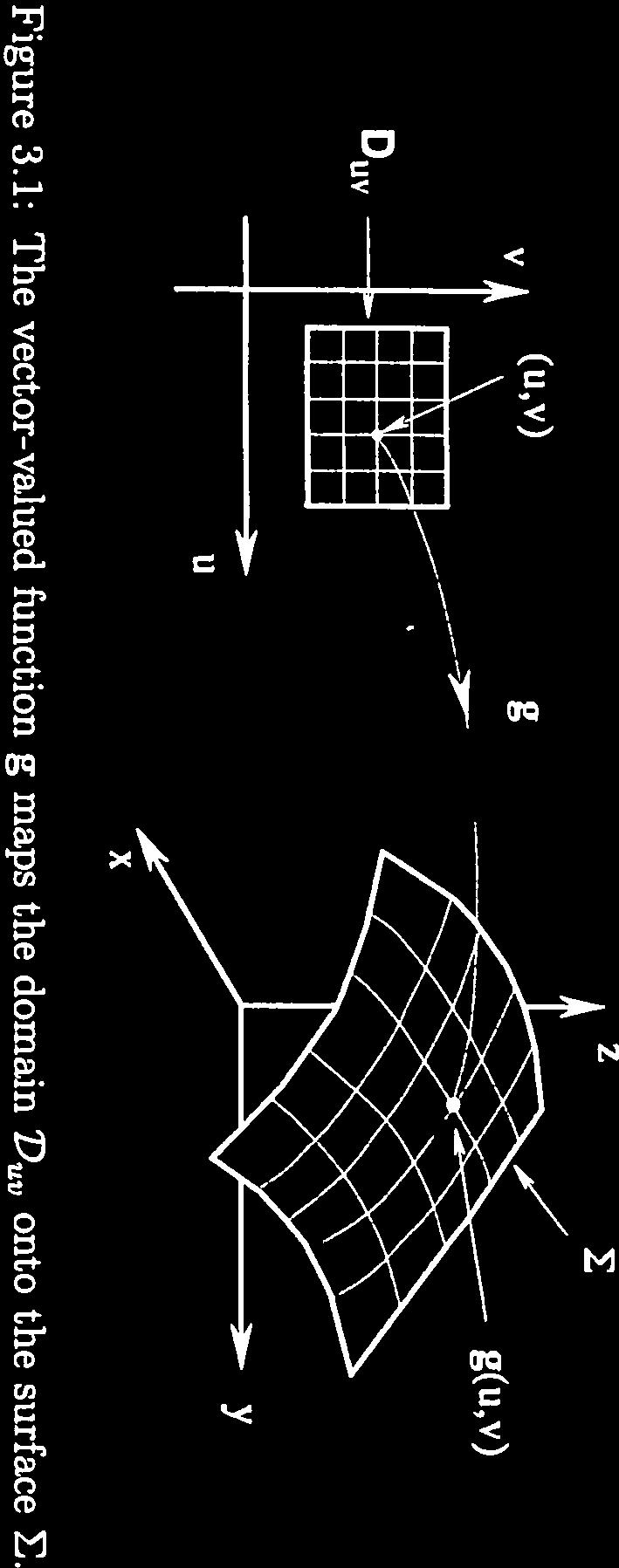
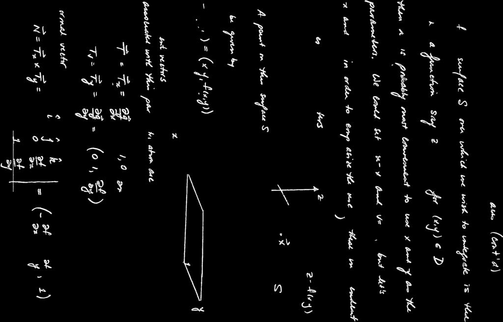
1 Lecture 16 urface Integrals (cont d) urface integration via parametrization of surfaces Relevant section of AMATH 231 Course Notes: ection In general, the compuation of surface integrals will not be as easy as in the example given above. We shall have to resort to parametrizing the surface and then expressing the surface integrals from (1) and (2) as integrations over these parameters. We shall need two parameters, say u and v, to define, because is 2-dimensional. is the set of parameter values (u,v) needed to define. The parameterization will be denoted by (to conform with the AMATH 231 Course Notes) g(u,v) = (x(u,v),y(u,v),z(u,v)) (x 0,y 0,z 0 ) = (x(u 0,v 0 ),y(u 0,v 0 ),z(u 0,v 0 )) Our goal: We want to write and f d = F ˆN d = f(g(u,v)) }{{} f evaluated } {{ } dudv may need on surface something here F(g(u,v)) ˆN(u,v) dudv

2

3

4 ome examples of surface parameterizations 1. phere with radius R, x 2 + y 2 + z 2 = R 2. Use the angles from spherical polar coordinates to identify a point on the sphere: Let u = θ, the azimuthal angle (angle with respect to xz plane). Let v = φ, the polar angle (angle with respect to z axis). Therefore, x(u,v) = R sinv cos u y(u,v) = R sinv sin u z(u,v) = R cos v, so that our parametrization may be expressed as g(u,v) = (R cos usin v,r sin usin v,rcos v). (1) The parameter space that defines the sphere: 0 u 2π,0 v π

5 2. Cylinder with x 2 + y 2 = a 2, 0 z b x(u,v) = acos u y(u,v) = asin u z(u,v) = v 0 u 2π, 0 v b The resulting parametrization: g(u,v) = (acos u,asin u,v). (2) 3. Cone with z 2 = x 2 + y 2, 0 z b If we set z = v (then 0 v b), then x = v cos u y = v sin u 0 u 2π,0 v b The resulting parametrization: g(u,v) = (v cos u,v sin u,v). (3) The region in parameter space defining the cone is shown below: 4. Planes are the simplest objects because they are flat. (a) Any plane parallel to a coordinate axis is trivial to parametrize. Consider, for example, the plane z = c. This means that z(u,v) = c for all (u,v). And x and y can simply be parametrized as x(u, v) = u and y(u, v) = v. The result: g(u,v) = (u,v,c). (4)

6 The other planes, e.g., x = a, are treated in similar ways. (b) As for the more general plane, Ax + By + Cz =, we simply express one coordinate in terms of the other two, e.g., z = C A C x B y (assuming that C 0). (5) C Please see Example 3.1 and Exercise 3.1 on pages of the AMATH 231 Course Notes for further discussion.

7 Normal vectors to surfaces from parametrizations Relevant section from AMATH 231 Course Notes: ections and Curve C 1 on the surface is obtained by fixing v = v 0 and letting u vary: c v0 (u) = g(u,v 0 ). Curve C 2 on the surface is obtained by fixing u = u 0 and letting v vary: c u0 (v) = g(u 0,v). Goal: To find N(u 0,v 0 ), the normal vector to at (x 0,y 0,z 0 ) = g(u 0,v 0 ). N is perpendicular to the tangent vectors T u and T v to curves c v0 (u) and c u0 (v), respectively. We can choose either of N = ±T u T v. Question: How do we find T u and T v? Answer: We know how to obtain tangent vectors to curves: Take derivatives w.r.t. parameter: T u = c v0 (u) = u g(u,v) v=v 0 T u (u 0,v 0 ) = = u g(u,v) (u,v) = (u 0,v 0 ) x, y u u (u 0,v 0 ) (u 0,v 0 ), z u (u 0,v 0 )

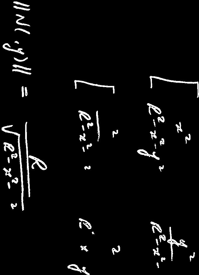
8 Likewise, T v (u 0,v 0 ) = u g(u,v) (u 0,v 0 ) x = v (u 0,v 0 ), y v (u 0,v 0 ), z v (u 0,v 0 ) (You require two vectors one involves u, the other v Now compute normal vectors: because you have two parameters u, v.) N(u 0,v 0 ) = ±T u (u 0,v 0 ) T v (u 0,v 0 ) = ± Note that all derivatives are evaluated at (u 0,v 0 ). î ĵ ˆk x u x v y u y v z u z v (u 0,v 0 ) Example: phere with radius R, x 2 + y 2 + z 2 = R 2. Parameterize as (u = θ,v = φ) (spherical coordinates). g(u,v) = (R cos } usin {{ v},rsin } usin {{ v},rcos }{{} v) x y z 0 u 2π, 0 v π Need to compute T u and T v : i j k T u T v = R sin usinv R cos usin v 0 R cos ucos v R sinucos v Rsin v = ( R 2 cos usin 2 v, R 2 sin usin 2 v, R } 2 sin 2 usin v cos v {{ R 2 cos 2 usin v cos v } ) simplifies to R 2 sin v cos v = Rsin v (R cos usin v,rsin usin v,r cos v) }{{} g(u,v) = Rsin v g(u,v)

9 For the outward normal, choose N = T u T v (or T v T u ) = R sinv g(u,v) Note that sin v 0 for v [0,π] as shown below on the left. The resulting outward normal N is sketched on the right. 0 v π Let us now compute the magnitude of this normal vector: N = R sin v g(u,v) = R 2 sin v, (6) where we have used the fact that g(u,v) = R since the point g(u,v), by construction, lies on a surface of sphere R. You may now be wondering why the magnitude of this normal vector is not constant; in particular, why would it be changing with the spherical polar angle v (angle between radial vector g and the z-axis). The answer is that the R 2 sinv factor provides another piece of information that necessary to translate the integration over the sphere to an integration in uv parameter space. It is the conversion factor, or Jacobian between an infinitesimal element of area da in the uv parameter space (shown at the left below) and the actual element of area d on the sphere (shown at the right). We ll show this below.

10 Lecture 17 urface integrals (cont d) urface integrals of scalar functions Relevant section from AMATH 231 Course Notes: 3.1.3, Let f(x,y,z) be defined over a surface. We want to integrate f over. In the spirit of calculus : The partitioning of on the left defines a partitioning of shown on the right. Pick sample points (u k,v k ), a subset of an appropriate square. Each of these points defines a point (x kl,y kl,z kl ) = g(u kl,v kl ). Evaluate f at (x kl,y kl,z kl ). Goal: But we don t know what kl is! f(x kl,y kl,z kl ) kl kl

11 Approximate kl by kl the area of a flat plane that covers kl that is tangent to somewhere in kl. o = f(x kl,y kl,z kl ) kl o what is kl? The area of the flat tangent plane piece. P Q = velocity wrt u u = T u (u 0,v 0 ) u (cat) imilarly, P = T v (u 0,v 0 ) v (dog) o the area of the parallelogram P Q R is = (cat) (dog) sin θ = T u T v sin θ u v = T u T v u v The final result is = N(u 0,v 0 ) u v f(...) = }{{} n,m partition f(x,y,z ) N(u,v ) u v

12 f d = u,v f evaluated on surface {}}{ f(g(u,v)) N(u,v) dudv }{{} dv du }{{} d element of area This is the formula for computing surface integrals of scalar-valued functions. Let us now work out a few surface integrations using the result stated at the end of the previous section. Example 1: urface area of a sphere with radius R. We shall use the parametrization introduced previously: g(u,v) = (x(u,v),y(u,v),z(u,v)) = (R cos usin v,r sinusin v,r cos v) where v = θ, u = φ, 0 v π, 0 u 2π. Recall that N = ±T u T v We choose T v T u since it is the outward normal. Previously, we computed the magnitude of this normal vector to be N(u,v) = R 2 sin v. (7) Let us now investigate the signifance of this result. In the figure below, on the left, the infintesimal element of area da produced by infinitesimals du and dv does not vary as we move around the rectangle in uv space. But the resulting element of area d does vary on the sphere. For example, the closer you are to the top of the sphere (i.e., the North Pole ), the smaller the element ds because the lines of constant v, i.e., the lines of longitude, are coming together as we approach the pole. This is reflected in the sinv term. As v 0, the element of area d gets smaller and smaller. da = dudv d = N(u,v) dudv }{{} Jacobian In fact, you have already seen this factor: it appears in the volume element dv in spherical polar coordinates. The only difference is that the R above, which is a fixed value since we are considering

13 a spherical shell becomes the lower case r in 3 spherical polar coordinates, since we also integrate over this variable. In order to compute the surface area of the sphere, we choose f(x,y,z) = 1. Then f d = d = A But f d o what is N(u,v) da for our problem? f(g(u,v)) N(u,v) da }{{} dudv }{{} dvdu We have to integrate N(u,v) = R 2 sin v over 0 u 2π, 0 v π. 2π π N(u, v) da = } R 2 {{ sin v} dvdu }{{} 0 0 }{{} N(u,v) da parameters Inner Integral: Outer Integral:. that generate π π R 2 sin v dv = R 2 ( cos v) 0 0 2π 2π 2R 2 du = R 2 (u) 0 0 = 2R 2 = 4πR 2 This agrees with our result for the area of a spherical surface of radius R. Example 2: Given a thin hemispherical shell, radius R, positioned as shown below. Find its centroid (0,0,z). z = z d d Here, the denominator d is the surface area of the hemisphere which is 2πR 2.

14 We need to compute z d. z d }{{} = parametrization g(u, v) z(u, v) N(u, v) da For z(u,v), we now have to express z on the surface in terms of u and v. z(u,v) = R cos v Note that we are integrating over the upper hemisphere, so the ranges of the parameters will be 0 u 2π (as for the sphere) but 0 v π/2 (unlike the sphere). Inner integral: = 2π 0 π 2 0 R} cos {{ v} z } R 2 {{ sinv} N(u,v) Jacobian 2π R 3 cos v sin v dv = R 3 ( sin2 v) 0 dvdu π 2 = 1 2 R3 Outer integral: 1 2π 2 R3 0 du = 1 2 R3 (u) 2π 0 = πr 3 z = 1 2 πr3 πr 2 = R 2 (half-way up) Note: You may wish to compare this result to the centroid of the solid hemisphere, z = 3 8R, which can be found by integration in 3 spherical polar coordinates.

15 Example 3: Compute the integral x2 z d over the cylinder g(u,v) = (cos u,sin u,v), 0 u 2π, 0 v 1. tep 1: Parameterization: Given. tep 2: Compute N(u,v) via T u, T v. T u = r ( x u = u, y u, z ) = ( sin u,cos u,0) u T v = r v = (0,0,1) i j k T u T v = sin u cos u 0 = (cos u,sin u,0) = N(u,v) Top view: As expected, the normal vector N is parallel to the xy-plane (since it has zero z-component) and points radially outward from the cylindrical surface. Note also that N(u,v) = 1. We now use the parametrizations x = cos u and z = v in the integrand to give x 2 z d = 1 2π 0 0 cos 2 uv dudv = π 2. (8) The above integral is particularly convenient to compute since it is separable, i.e., the u- and v- dependent terms can be separated so that that the double integral over u and v can be expressed as a product of integrals over u and v: 1 2π 0 0 ( 1 cos 2 uv dudv = 0 ) ( 2π ) v dv cos 2 udu = 0 ( ) 1 (π) = π 2 2. (9)

16 Example 4: Compute the area of the cylinder used in Example 3. We simply have to compute the surface integral d. Using the parametrization from Example 3 and the fact that N(u,v) = 1, the surface area is given by d = 1 2π 0 0 dudv = 2π. (10) This result is confirmed if we take the cylinder, cut it open by means of a vertical cut, and flatten it out. The result is a rectangle with dimensions 2π and 1. The area of this rectangle is 2π.

17

18

19

20

21

22

23

24

25

26

27

28 urface integrals (cont d) urface integrals of vector functions and flux Relevant section from AMATH 231 Course Notes: 3.2.2, p. 77 We return to the concept of the flux of a vector field F. Now, however, we are concerned with the flux of F through s surface. The unit normal ˆN to at (x, y, z) is usually directed outward (as dictated by the physical problem). (x, y, z) is centered in an infinitesimal element d of area on. The amount of F pointing in the direction of ˆN is the projection of F in the direction of ˆN, i.e., F ˆN. The (infinitesimal) flux of F through the surface element d is F ˆN d. To obtain the total flux through the surface, we must integrate over all elements d centered at (x,y,z). We denote this vector surface integral as follows F ˆN d. (11) In order to understand this idea better, let us examine a particular physical application of the flux integral.

29 Flux in terms of fluid flow First, consider a region that lies in the xy-plane as sketched below. uppose that a fluid is passing through this region. For the moment, we assume that motion of the fluid is perpendicular to region, travelling in the direction of the positive z-axis. Moreover, we assume that the speed of the fluid particles crossing is constant throughout the region. As such, we are assuming that the velocity field of the fluid is F = vk, v > 0 (constant). (12) z F = vk x y We first ask the question: How much fluid flows through region during a time interval t? Consider a tiny rectangular element of area A = x y centered at a point (x,y) in. After a time t, the fluid particles situated in this element will have moved a distance v t upward. The volume of fluid that has passed through this element A on is the volume of the box of base area A and height v t: v t A. (13) This box is sketched below. z F = vk x v t y A The total volume V of fluid that has passed through region over the time interval t is

30 obtained by summing up over all area elements A in : V = v t da = v ta(), (14) where A() denotes the area of. Of course, this is a rather trivial result: the volume of fluid passing through is simply the volume of the solid of base area A() and height v t. ividing both sides by t, we have V t = va(). (15) In the limit t 0, we have the instantaneous rate of change of the volume of fluid passing through region, or simply the rate of fluid flow through region : V (t) = va(). (16) This quantity is the flux of the vector field v through region. Now suppose that the fluid is now moving at a constant speed v through region but not necessarily at right angles to it, i.e., not necessarily parallel to its normal vector k. We shall suppose that v = v 1 i + v 2 j + v 3 k, v = v (17) and let γ denote the angle between v and the normal vector k. In this case, the fluid particles that pass through the tiny element A after a time interval t form a parallelopiped of base area A and height v cos γ t, as sketched below. z F x γ v cos γ y A The volume of this box is v cos γ t A. (18) (Think of this tower of fluid as a deck of playing cards that has been somewhat sheared. When you slide the cards back to form a rectangular arrangement, the height of the deck is vδt cos γ.)

31 The total volume V of fluid that has passed through region over the time interval t is obtained by summing up over all area elements A in : V = v cos γ t da = v cos γ ta(), (19) ividing both sides by t, we have V t = v cos γa(). (20) In the limit t 0, we obtain the flux of the vector field v through region : We shall rewrite this flux as follows, V (t) = v cos γa(). (21) V (t) = v ˆN A(), (22) since ˆN = k is the normal vector to surface. Note that this general case includes the first case, γ = 0. And in the case that γ = π/2, there is no flow through the region, so the flux is zero. Of course, the above results have been rather trivially obtained since (i) the vector fields are constant and (ii) the region is flat. Let us now generalize the first case, i.e., the vector field v is assumed to be nonconstant over region, i.e., v(x,y) = v 1 (x,y)i + v 2 (x,y)j + v 3 (x,y)k. (23) In this case, the total volume V of fluid that has passed through region over the time interval t is obtained by summing up over all area elements A in : V = t v(x,y) ˆN da = t v 3 (x,y) da. (24) Once again dividing by t and taking the limit t 0, we obtain the total flux of v through region : V (t) = v(x,y) ˆN da (25) Now suppose that we were concerned with rate of mass flow through region. The amounts/volumes of fluid examined earlier would be replaced by amounts of mass flowing through a surface element. This means replacing the velocity vector field v by the momentum field F = ρ v, where ρ is the mass density. The rate of transport of mass through region would then be given by M (t) = F(x,y) ˆN da = ρ(x,y) v(x,y) ˆN da (26) This concludes our discussion of this simple problem involving fluid flow through a flat surface.

32 Generalization to arbitrary surfaces We now wish to generalize the above result to general surfaces in R 3. In other words, we do not require the surface to be flat, as was region in the plane, but rather a general surface in R 3 for example, a portion of a sphere, or perhaps the entire sphere. In the spirit of calculus, we divide the surface into tiny infinitesimal pieces d. We then construct a normal vector ˆN to each surface element d at a point in d, as sketched below. We then form the dot product of the vector field F at that point with the normal vector ˆN. This will represent the local flux of F through the surface element d. To obtain the total flux through the surface, we add up the fluxes of all elements d an integration over that is denoted as F ˆN d. (27) This is the flux of F through surface. Note that in some books, especially Physics books, the vector surface integral is denoted as F d. (28) Here, the infinitesimal surface area element is a vector that is defined as d = ˆN d, (29) where d is the infinitesimal surface element and ˆN is the unit normal vector to the surface element. In other books, the infinitesimal surface element is denoted as da = ˆNd, so that the flux integral is denoted as F da. (30)

33 Practical computation of flux integrals The integrand in a vector surface integral, F ˆN, will generally depend on the x,y,z. ince these coordinates are restrcted to the surface of interest, they, hence the integrand, will depend on u and v (i.e., (x(u,v),y(u,v),z(u,v))). As we saw in the introduction to this section, in some special cases that occur in physics, e.g. gravity, electricity/magnetism, the vector fields and the surfaces are spherically symmetric. In such cases, we can compute fluxes in a rather straightforward way using the definition of the flux integral. In general, however, the computation of flux integrals may not be as straightforward as for these elementary examples. As in the case of surface integrals for scalar functions, we ll have to use the parametrization of the surface. Notice that in the total flux integral, F ˆN d the integrand F ˆN is a scalar call it f(x,y,z) so that the flux integral becomes = f d But we know how to compute surface integrals of scalar functions! If we parametrize the surface, (g(u,v),(u,v) uv ), then f d = f(g(u,v)) N(u,v) da (31) uv Here, f is the dot product F ˆN on surface : f(g(u,v)) = F(g(u,v)) }{{} ˆN(u, v) }{{} F on surface appropriate unit normal on What is ˆN? o Equation (31) becomes = ˆN(u,v) = N(u,v) N(u,v) F(g(u,v)) N(u, v) N(u,v) N(u,v) da

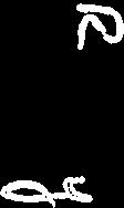
34 The final result is: F ˆN d = F(g(u,v)) N(u,v) da uv The vector surface integral is translated into a surface integral involving the scalar function F ˆN. The integration on the right-hand side is performed over the region in uv parameter space, uv, that generates the surface. ome of the examples which are presented below will involve either spherical surface R either a part of it or its entirety of radius R and centered at (0,0,0). Recall that the parametrization of this surface is given by g(u,v) = (R sin v cos u,rsin v sinu,r cos v), 0 u 2π, 0 v π. (32) Also recall from our earlier work that the outward normal associated with this parametrization was given by N = T v T u = R sin v g(u,v). (33) 1. As a kind of warmup, let us first compute the total flux of the vector field F = k = (0,0,1) through the circular planar region on the xy-plane, = {(x,y,0) x 2 + y 2 R 2 }. (34) The boundary of this region is the intersection of the spherical surface R with the xy-plane. The situation is sketched below. z x y

35 The computation of the flux of F through this region is quite straightforward since the surface is a plane and the vector field is constant. In fact, the surface lies on the xy-plane which implies that its unit normal vector ˆN = k. We can simply use Eq. (21) from the earlier part of this lecture: F ˆN da = (0,0,1) (0,0,1)dA = da = πr 2. (35) 2. Now let us compute the total flux of the same vector field, F = k = (0,0,1), but through the upper hemispherical surface of R, as sketched below. z upper hemisphere of R x y We must compute the surface flux integral, F ˆN d = F(g(u,v)) N(u,v)dA uv The integrand must be evaluated over the surface. Here, F(g(u,v)) = (0,0,1) so that F(g(u,v)) N(u,v) = (0,0,1) R sin v(r sin v cos u,r sin v sin u,rcos v) = R 2 sin v cos v. Now integrate over surface, keeping in mind that we re integrating only over the upper hemisphere, so that 0 v 1 2 π: F ˆN d = π/2 2π 0 0 R 2 sin v cos v dudv π/2 = 2πR 2 sin v cos v dv 0 1 = (2πR 2 ) 1 2 π 2 sin2 v 0 }{{} = πr 2.

36 Note that we obtain the same result as in Example 1. The net flux of the fluid passing through the hemispherical surface is the same as the flux of the fluid passing through the projection of this surface onto the xy-plane. 3. Let us now compute the total outward flux of the vector field F = k = (0,0,1) of Examples 1 and 2 through the entire spherical surface R. It appears that the amount of vector field entering the sphere from the bottom is equal to the amount that is exiting at the top. One would conjecture, then, that the total flux across the sphere is zero. Once again, we must compute the flux integral, F ˆN d = F(g(u,v)) N(u,v)dA uv The integrand must be evaluated over the surface. Here, F(g(u,v)) = (0,0,1), so that F(g(u,v)) N(u,v) = (0,0,1) R sin v(r sin v cos u,r sin v sin u,rcos v) = R 2 sin v cos v. Now integrate over entire spherical surface: In this case 0 v π: π 2π F ˆN d = R 2 sin v cos v dudv 0 0 π = 2πR 2 sin v cos v dv 0 π = (2πR 2 ) 1 2 sin2 v 0 }{{} =0 = 0. This was as expected net outward flow through the top is equal to the net inward flow through the bottom. 4. Compute the total outward flux of the vector field F = zk = (0,0,z) through the spherical surface R.

37 The arrows in the vector field get longer as you move away from the xy-plane. Moreover, for z > 0, they point upward and for z < 0, they point downward. Therefore, there is a net outward flow from the xy-plane through the surface. We expect a nonzero, in fact, positive outward flux here. On the surface, F(g(u, v)) = (0, 0, z(u, v)) so that = (0,0,R cos v), F(g(u,v)) N(u,v) = (0,0,R cos v) R sin v(r sin v cos u,r sinv sin u,rcos v) = R 3 cos 2 v sin v. The flux is therefore given by F ˆN d = π 2π 0 0 R 3 cos 2 v sin v dudv π = 2πR 3 cos 2 v sin v dv 0 π = (2πR 3 ) 1 3 cos3 v 0 = (2πR 3 )( 2 3 ) = 4 3 πr3. By symmetry, you will find the same result for F = xi or F = yj (i.e., same type of vector field, just in a different direction). Note: The fact that the total flux for these vector fields is equal to the volume of the sphere is not a coincidence, as we ll see in the next lecture. It is a consequence of the celebrated ivergence Theorem.

38 Gauss ivergence Theorem in R 3 Relevant section of AMATH 231 Course Notes: ection In this section, we are concerned with the outward flux of a vector field (through a smooth/piecewise smooth) surface that encloses a region V R 3. Typically, in physics such surfaces are spheres, boxes, parallelpipeds or cylinders. This is the subject of the celebrated Gauss ivergence Theorem, the three-dimensional version of the ivergence Theorem in the Plane of a previous lecture. The Gauss ivergence Theorem is one of the most important results of vector calculus. It is not as important for computational purposes as for conceptual developments. It provides the basis for the important equations in electromagnetism (Maxwell s equations), fluid mechanics (continuity equation) and continuum mechanics in general (heat equation, diffusion equation). It is sufficient to consider a somewhat simplified version of the general ivergence Theorem. A simplified version of the ivergence Theorem: Let be a nice (i.e., piecewise smooth) closed and nonintersecting surface that encloses a region R 3, such that an outward unit normal vector ˆN exists at all points on. Also assume that a vector field F and its derivatives are defined over region and its boundary. The ivergence Theorem states that: F ˆN d = divfdv. (36) }{{}}{{} surface integral volume integral Once again, we have assumed that divf exists at all points in V. You have already seen a version of this theorem the two-dimensional ivergence Theorem in the plane. It expressed the total outward flux of a 2 vector field F through a closed curve C in the plane as an integral of the divergence of F over the region enclosed by C: F ˆN ds = C div F da. (37) Examples: In what follows, unless otherwise indicated, the surface is an arbitrary surface in R 3 satisfying the conditions of the ivergence Theorem.

39 1. The vector field F = k = (0,0,1). This vector field could be viewed as the velocity field of a fluid that is travelling with constant speed in the positive z-direction: y x z The divergence of this vector field is zero: div F = x (0) + y (0) + (1) = 0. (38) z More importantly, it exists at all points in R 3, i.e., there are no singularities, so that we may employ the ivergence Theorem. Therefore, for any surface enclosing a region, we have F ˆN d = divfdv = 0 dv = 0. (39) In other words, the total outward flux of F over the surface is zero. In terms of the fluid analogy, fluid is entering the region through surface from the bottom at the same rate that it is leaving it at the top. There is no creation of extra fluid anywhere inside region that would cause a nonzero flux. 2. The vector field F = zk = (0, 0, z). A sketch of the vector field is given below. y x z This field could be viewed as the velocity field of a liquid that originates from the xy-plane and travels upward and downward away from it. As it moves away, it accelerates, since the velocity is proportional to the distance from the xy-plane.

40 The divergence of this field is div F = x (0) + y (0) + (z) = 1. (40) z Once again, the divergence exists at all points in R 3. Therefore, by the ivergence Theorem the volume of region. F ˆN d = R divfdv = 1 dv = V (), (41) Note that the same result for the flux, i.e., Eq. (41), would be obtained for the following vector fields: (i) F = xi, (ii) F = yj, (42) since the divergence of each of these vector fields is 1. And the list does not stop here. Consider the set of all vector fields of the form F = c 1 xi + c 2 yj + c 3 zk, where c 1 + c 2 + c 3 = 1. (43) In all cases, we have div F = 1, so that the total outward flux of each of these fields through the surface is V (), the volume of region. 3. The vector field F = z 2 k = (0,0,z 2 ). Here, all arrows of F point upward, as sketched below. y x z This could be visualized as fluid that emanates from the xy-plane to travel upward, accelerating as it moves away from the plane, along with fluid that approaches the xy-plane from below, decelerating as it gets closer. The divergence of F is div F = x (0) + y (0) + z (z2 ) = 2z (44)

41 Therefore, by the ivergence Theorem F ˆN d = divfdv = 2 z dv. (45) The value of this integral will depend on the region. In principle, if we knew the region, we could integrate over it, using the techniques for integration in R 3 developed earlier in the course. There is one interesting point regarding this integral: It is related to the z coordinate of the centroid of region. Recall that z = z dv dv. = z dv, (46) V () implying that Therefore, Eq. (45) becomes z dv = V () z. (47) F ˆN d = 2 zv (). (48) Note that if the surface is located in the upper half-plane, i.e., z > 0, then z > 0, implying that the total outward flux is positive. However, if the surface is located in the lower half-plane, i.e., z < 0, the total outward flux is negative. Why is this so? And why would the total outward flux be directly proportional to the volume V () of the region enclosed by the surface?