Prerequisite Material

Transcription

1 Prerequisite Material Study Populations and Random Samples A study population is a clearly defined collection of people, animals, plants, or objects. In social and behavioral research, a study population usually consists of a specific group of people. Some examples of human study populations are all UCSC freshman, all California public school teachers, all spouses of Alzheimer s patients in Minnesota, and all preschool children in Chicago. Quantitative Measurements In addition to specifying the study population of interest, a researcher will specify some attribute to measure. When studying human populations, the attribute of interest might be a specific type of academic ability, a memory task, a personality trait, some particular behavior (e.g., hours of TV watching, willingness to assist a stranger), an attitude, an interest, an opinion, or a physiological measure (e.g., heart rate, blood pressure, blood flow in specific parts of the brain). To measure some attribute of a person s behavior is to assign a numerical value to that person. These measurements can have different properties. A ratio scale measurement has the following three properties: 1) a score of 0 represents a complete absence of the attribute being measured, 2) a ratio of any two scores correctly describes the ratio of attribute quantities, and 3) a difference between two scores correctly describes the difference in attribute quantities. Suppose a person s heart rate is measured. This measurement is a ratio scale measurement because a score of 0 beats per minute (bmp) represents a stopped heart and a heart rate of, say, 100 bpm is twice as fast as a heart rate of 50 bpm. In addition, the difference between two heart rates of, say, 50 and 60 bmp describes the same increase in heart rate as the difference between 70 and 80 bpm. With interval scale measurements, a score of 0 does not represent a complete absence of the attribute being measured and a ratio of two scores does not correctly describe the ratio of attribute quantities, but a difference between two interval scale scores will correctly describe the difference in attribute quantities. Most measurements of 1

2 psychological attributes are not ratio scale measurements but are assumed to be interval scale attributes. For instance, the Beck Depression Inventory (BDI) is scored on a 0 63 scale with higher scores representing higher levels of depression. However, a BDI score of 0 does not indicate a complete absence of depression nor does a BDI score of, say, 40 represent twice the amount of depression as a BDI score of 20. It is assumed that a difference between two BDI scores correctly describes the difference in depression levels so that a person who initially obtained a BDI score of, say, 30 and then obtained a score 20 after therapy is assumed to have the same level of improvement as a person who initially scored 25 on the BDI and dropped to 15 after therapy. Ratio and interval scale measurements will be referred to simply as quantitative scores. Each member of the population could be measured on more than one attribute. Consider the simplest case where there are only two attributes of interest so that two quantitative scores will be assigned to each person. The two quantitative scores for person i will be denoted as y i and xi. The y i scores and xi scores are expected to vary across people and are therefore referred to as variables. In applications where variable x is believed to predict variable y, x will be called the predictor variable (also referred to as an explanatory variable or independent variable) and y will be called the response variable (also referred to as an outcome variable or a dependent variable). Population Parameters A population parameter is an unknown numeric value that describes the measurements that could have been assigned to all N members of a specific study population. The value of a population parameter could be used to make an important decision or to advance knowledge in some area of research. The population mean is a parameter that describes the center of a distribution of quantitative scores. If each person in the study population was assigned scores y i and x i (i = 1 to N) the population mean of the y scores (denoted as μ y ) and the population mean of the x scores (denoted as μ x ) are N μ y = i=1 y i /N μ x = i=1 x i /N (1.1) where y i and x i are the quantitative scores for person i. N 2

3 The population standard deviation is a parameter that describes the variability of quantitative scores. The population standard deviations of the y scores (denoted as σ y ) and x scores (denoted as σ x ) are σ y = (y i μ y ) 2 N i=1 σ x = N (x i μ x ) 2 i=1 (1.2) N Note that the standard deviation cannot be negative. The squared standard deviation occurs frequently in statistical formulas and is called the variance. N The population covariance is a parameter that describes the linear association between two quantitative variables. The population covariance between variables y and x is defined as N σ yx = (y i μ y )(x i μ x ) i=1 (1.3) N A covariance will be positive if above average y scores tend to be paired with above average x scores and below average y scores tend to be paired with below average x scores. A covariance will be negative if above average y scores tend to be paired with below average x scores and below average y scores tend to be paired with above average x scores. Although the sign of a covariance correctly describes the direction of the relation (positive or negative), the numerical value of a covariance is not a useful description of the strength of the association between the two variables because its value depends on the standard deviations of both x and y. A more useful measure of association is the population Pearson correlation coefficient ρ yx = σ yx σ y σ x (1.4) which can range from -1 to 1. A ρ yx value of -1 or 1 indicates a perfect linear association between x and y, and a ρ yx value of 0 indicates no linear association between x and y. The coefficient of determination is equal to the squared Pearson correlation (ρ 2 yx ) and describes the proportion of variance in one variable that is linearly associated with (or can be predicted from) the other variable. 3

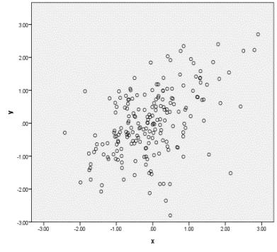
4 The association between two quantitative variables can be represented graphically in a scatterplot. An example of a scatterplot of verbal and quantitative SAT scores is given below for a study population of all 3,138 high school students who applied to a particular university. The covariance between verbal and quantitative SAT scores in this study population is positive because students with above average quantitative SAT scores tend to have above average verbal SAT scores, and students with below average SAT quantitative scores tend to have below average verbal SAT scores. A scatterplot provides useful information about the direction of the relation between y and x, the strength of the relation between y and x, and shape (linear or curvilinear) of the relation between y and x. A scatterplot also can reveal anyone with an unusual combination of y and x scores. Random Samples and Parameter Estimates In applications where the study population is large or the cost of measurement is high, the researcher may not have the necessary resources to measure all N people in the study population. In these applications, the researcher could take a random sample of n people from the study population of N people. In studies where random sampling is used, the study population is defined as the population from which the random sample was obtained. A random sample of size n is selected (usually using a computer program) in 4

5 such a way that every possible sample of size n will have the same chance of being selected. Population means, standard deviations, covariance, and correlation can be estimated from a random sample of size n. The sample means n μ y = i=1 y i /n μ x = i=1 x i /n (1.5) estimate μ y and μ x. The sample standard deviations n σ y = (y i μ y) 2 n i=1 σ x = n (x i μ x) 2 i=1 (1.6) estimate σ y and σ x. n 1 n 1 The sample covariance n (y i μ y)(x i μ x) σ yx = i=1 (1.7) n 1 is an estimate of σ yx, and the sample Pearson correlation coefficient ρ yx = σ yx σ yσ x (1.8) is an estimate of ρ yx. Squaring Equation 1.8 gives an estimate of ρ 2 yx. Examples of scatterplots for several different correlation values are illustrated on the following page in Figure 1. It is important to examine the scatterplot patterns for different correlation values in Figure 1 so that a scatterplot can be visualized for any given correlation value. After examining Figure 1, most researchers would agree that a correlation less than.3 represents weak and possibly an unimportant relation between the two quantitative variables. To save space, most research articles report only the value of the correlation. The reader must then be able to visualize the general form of the scatterplot for a reported correlation value and subjectively assess importance of the relation. 5

6 ρ yx = 0 ρ yx =.1 ρ yx =.2 ρ yx =.3 ρ yx =.4 ρ yx =.5 ρ yx =.6 ρ yx =.7 ρ yx =.8 ρ yx =.9 ρ yx =.95 ρ yx =.99 Figure 1. Scatterplots for different correlation values 6

7 Normal Distribution A normal distribution is bell-shaped and symmetric as illustrated in the graph below. If a distribution of scores is approximately normal, about 68% of the scores will be within one standard deviation from the mean, about 95% of the scores will be within two standard deviations from the mean, and almost all of the scores will be within three standard deviations of the mean. One standard deviation from the mean can be visualized in a normal distribution because this is the point (called an inflection point) where the curve changes from bending down to bending up. The asymmetry in a set of quantitative scores can be described using a coefficient of skewness. Let z i = (y i μ y)/σ y. An estimate of the coefficient of skewness is equal to n i=1 z 3 i /n. A skewness coefficient will equal zero if the scores are perfectly symmetric. A skewness coefficient will be positive if the scores are skewed to the right and negative if the scores are skewed to the left. R provide a test of the null hypothesis that the population skewness coefficient is zero. If the p-value for the test of zero skewness is less than.05, the researcher can conclude that the population normality assumption has been violated and that the population scores are skewed to the left or to the right according to the sign of the sample skewness coefficient. However, a p-value greater than.05 should not be interpreted as evidence that the normality assumption has been satisfied. The population distribution of quantitative scores can be non-normal even if the distribution is symmetric. The coefficient of kurtosis describes the degree to which a distribution is more or less peaked or has shorter or longer tails than a normal distribution. The kurtosis of a distribution can be described by a coefficient of kurtosis which is equal to 3 in a normal distribution. The kurtosis coefficient has a theoretical 7

8 lower limit of 1 with no upper limit. An estimate of the coefficient of kurtosis is equal to n i=1 z 4 i /n. Subtracting 3 from the kurtosis coefficient, so that it will equal 0 in normal distributions, is called excess kurtosis. Leptokurtic distributions have excess kurtosis greater than 0 and are more peaked or have longer tails than a normal distribution. Platykurtic distributions have excess kurtosis less than 0 and are less peaked or have shorter tails than a normal distribution. R provide a test of the null hypothesis that the population excess kurtosis is zero. If the p-value for the test of zero excess kurtosis is less than.05, the researcher can conclude that the population normality assumption has been violated and that the population scores are either leptokurtic or platykurtic according the value of the sample kurtosis coefficient. However, a p-value greater than.05 should not be interpreted as evidence that the normality assumption has been satisfied. Linear Regression Model A linear regression model can be used to describe a linear relation between x and y in a random sample of participants. There are two basic versions of the linear regression model: a random-x model and a fixed-x model. In the random-x model, each participant in a random sample is assigned a pair of x and y scores. In this situation, the x values observed in the sample will not be known in advance. In the fixed-x model, the values of x are predetermined by the researcher. A fixed predictor variable is also called a factor. The fixed predictor variable can be a treatment factor with values to which participants are randomly assigned. For instance, in an experiment where hours of training is a quantitative treatment factor with predetermined values x = 10, 20, 30, and 40 hours, the researcher would randomly divide the sample into four groups with each group receiving 10, 20, 30, or 40 hours of training. A fixed predictor variable also can be a classification factor with values that represent existing characteristics of the study population. For instance, in a nonexperimental design a researcher might decide to sample children who are x = 5, 7, and 12 years old. A random-x model implies a nonexperimental design, but a fixed-x model could be used in either an experimental design or a nonexperimental design. The following linear regression model describes an assumed linear relation between x and y for a randomly selected person y i = β 0 + β 1 x i + e i (1.9) 8

9 where β 0 is the population y-intercept and β 1 is the population slope. The value β 0 + β 1 x i is the predicted y score for person i, and e i = y i β 0 + β 1 x i is the prediction error for person i. The variance of the prediction errors is denoted as σ e 2. The above model is referred to as a simple linear regression model because it has only one predictor variable. In a random-x model or a fixed-x model for nonexperimental designs, β 1 describes the change in the predicted y score associated with any 1-point increase in x. In the fixed-x model for experimental designs, β 1 describes the change in the population mean of y caused by any 1-point increase in x. The following values of β 0 and β 1 minimize the sum of the squared prediction errors N 2 ( e i ) in the study population i=1 2 β 1 = σ yx /σ x (1.10) β 0 = μ y β 1 μ x (1.11) Rearranging Equation 1.4 gives σ yx = ρ yx σ y σ x and substituting this expression for σ yx into Equation 1.10 gives β 1 = ρ yx (σ y /σ x ) which shows that the value of β 1 depends on correlation between y and x and also the variability of x and y. The quantity β 0 + β 1 x i has two interpretations. In one interpretation, which applies to both random-x and fixed-x models, β 0 + β 1 x i is the predicted y score for a person with an x score equal to x i. In another interpretation, which is meaningful only in the fixed-x model, β 0 + β 1 x i is the population mean of y at x = x i. The population mean of y at x = x i is denoted as μ y xi. It follows that β 0 is the predicted y score for a person who has an x score of 0, and in the fixed-x model, β 0 is the population mean of y at x = 0. If 0 is not a plausible value for x, then the value of β 0 will not have a useful or meaningful interpretation. The formulas for estimating β 0 and β 1 from a random sample of size n are the same for the random-x and fixed-x models. The estimate of β 1 is β 1 = σ yx /σ x2 (1.12) and the estimate of β 0 is 9

10 β 0 = μ y β 1μ x (1.13) The estimated y-score for person i is y i = β 0 + β 1x i (which is also an estimate of μ y xi in the fixed-x model) and the estimated prediction error (also call a residual) for person i is e i = y i y i. Equations 1.12 and 1.13 are called least squares estimates because they are the unique values that minimize n i=1 e i 2. The linear equation y i = β 0 + β 1x i with least squares estimates of β 0 and β 1 is called a line of best fit. Some researchers prefer to center the predictor variable by subtracting μ x from each x score. When the predictor variable has been centered, μ x = 0 and then β 0 = μ y. Centering does not change the value of β 1. Define the standardized variables y* = (y μ y)/σ y and x* = (x μ x)/σ x. If Equations 1.12 and 1.13 are computed using y* and x*, then it can be shown that β 0 = 0 and β 1 = ρ yx. This result shows that a Pearson correlation can be interpreted as the change in y, in standard deviation units, that is associated with a 1 standard deviation increase in x. An estimate of the variance of the prediction errors in the study population (σ e 2 ) is σ e2 = n i=1 e i 2 n 2 (1.14) Taking the square root of Equation 1.14 estimates the residual standard deviation (σ e) which describes how accurately x can predict y. A small value of σ e indicates that the 2 estimated y-scores tend to be close to the observed y scores. The estimate of σ e (Equation 1.14) is also denoted as MSE. Dummy Coded Predictor Variable Consider a study with a two-level qualitative predictor variable, such as male and female or treatment A and treatment B. There are two population parameters of interest in this type of study: μ 1 is the population mean of y for level 1 of the predictor variable (e.g., male, treatment A), and μ 2 is the population mean of y for level 2 of the predictor variable (e.g., female, treatment B). A two-level qualitative predictor variable can be used in a regression model if the two levels are converted into numerical values. A dummy coded predictor variable sets x i = 1 for every participant in level 1 of the qualitative factor (e.g., male, treatment A) and x i = 0 for every participant in level 2 of the qualitative factor (e.g., 10

11 female, treatment B). If x i in Equation 1.9 is a dummy coded predictor variable, it can be shown that β 1 = μ 1 μ 2 and β 1 = μ 1 μ 2. Sampling Distributions Consider a study population consisting of N people. Imagine taking a sample of n people from this study population and then computing an estimate of some parameter such as β 1, ρ yx, or σ e2. Now imagine doing this for every possible sample of size n. The set of all possible sample parameter estimates, for samples of size n, is called a sampling distribution. If the mean of the sampling distribution for a particular parameter estimate is equal the population parameter value, the parameter estimate is said to be an unbiased estimate. The estimates of μ y, μ x, σ 2 e, and β 1 (Equations 1.5, 1.12, and 1.14) are unbiased estimates. If the mean of the sampling distribution for a particular estimate becomes closer to the population parameter value as the sample size increases, the estimate is said to be a consistent estimate. The estimate of ρ yx (Equation 1.8) is a consistent estimate. For all estimates we will consider, their sampling distributions will be closely approximated by a normal distribution if the sample size is sufficiently large. The sampling distribution for β 1 can be well approximated by a normal distribution in small samples, but the sampling distributions of ρ yx and σ e2 are not well approximated by the normal distribution unless the sample size is large. However, some estimates can be transformed (e.g., ln(σ e2 ) ) so that the sampling distribution of the transformed estimates is well approximated by a normal distribution in small samples. The standard deviation of a sampling distribution is called the standard error of the estimate. The variability of a sampling distribution decreases with larger sample sizes. Remarkably, the standard error of a sampling distribution can be estimated from a single random sample. The estimated standard error of a parameter estimate describes the accuracy of the parameter estimate. A small standard error value indicates that the parameter estimate is likely to be close to the population parameter value, and a large standard error value indicates that the parameter estimate could be very different from 11

12 the population parameter value. As one would expect, increasing the sample size will decrease the value of the standard error. Inferential Methods The values of population parameters can provide information to answer important research questions, but usually only sample estimates are available because the study population size is either too large or the measurement process is too costly. A sample estimate can be misleading because it can be larger or smaller than the population value (sampling error) and the direction of the sampling error will be unknown. Furthermore, the magnitude of the sampling error for a particular estimate will be unknown. Thus, the sample estimate might be too small or too large, and it might be close to or very different from the population parameter value. A parameter estimate combined with its standard error, both of which are computed from a random sample, can be used to make a claim regarding the value of the unknown population parameter. There are two general types of claims that can be made about a population parameter based on a sample estimate of the parameter and its standard error. One type of claim is in the form of a confidence interval. A confidence interval is a range of values that is believed to contain the population parameter value with some specified level of confidence. A 95% confidence level is often recommended for research that is intended for publication. The second type of claim is a hypothesis test where the goal might be to decide if the population parameter value is less than some specified value or greater than some specified value. The decision is accompanied with a statement about the probability of the decision being incorrect. Most scientific journals require the probability of an incorrect decision to be no greater than.05. Confidence intervals and hypothesis tests are referred to as inferential statistical methods because they use information from a random sample to make an inference about the value of some population parameter. Confidence Interval for β 1 A 100(1 α)% confidence interval for β 1 is β 1 ± t α/2;df SE β 1 (1.15) 12

13 where SE β 1= σ e 2 σ x2 (n 1) is the estimated standard error of β 1, t α/2;df is a two-sided critical t-value, and df = n 2. Note also that SE β 1 depends on the variance of the x scores with greater variability in the x scores resulting in a smaller value of SE β 1. This fact is useful in a fixed-x model for an experiment with a quantitative factor using a wider range of x values will provide a more accurate estimate of β 1. It can be shown that σ e2 = (n 1)σ y2 (1 ρ yx 2 ) n 2 determination (ρ yx 2 ). which illustrates how SE β 1 also depends on the coefficient of Confidence Interval for ρ yx An approximate confidence interval for ρ yx, which assumes a random-x model, is obtained in two steps. First, a 100(1 α)% confidence interval for a transformed correlation estimate is computed ρ yx ± z α/2 1 n 3 (1.16) where ρ yx = ln ([ 1 + ρ yx 1 ρ yx ])/2 is called the Fisher transformation of ρ yx, z α/2 is a critical twosided z-value, and 1 n 3 is the standard error of ρ yx. Let ρ L and ρ U denote the endpoints of Equation Reverse transforming the endpoints of Equation 1.16 gives the following lower confidence limit for ρ yx exp(2ρ L ) 1 exp(2ρ L ) + 1 (1.17a) and the following upper confidence limit for ρ yx exp(2ρ U ) 1 exp(2ρ U ) + 1. (1.17b) The sampling distribution of ρ yx is not well approximated by a normal distribution unless the sample size is very large or if ρ yx is close to zero. However, the sampling distribution of ρ yx is closely approximated by a normal distribution in small samples and virtually any value of ρ yx. In random-x models, a confidence interval for ρ yx might be more useful or easier to interpret than a confidence interval for β 1 in applications where there is no clear psychological meaning of specific y scores or x scores. 13

14 Confidence Interval for Coefficient of Determination 2 In the random-x model, a confidence interval for ρ yx can be obtained by simply squaring the endpoints of Equations 1.17ab if the confidence interval for ρ yx does not include 0. If 2 the confidence interval for ρ yx does include 0, then the lower limit for ρ yx is set to 0 and 2 the upper limit for ρ yx is equal to the largest squared endpoint. For instance, if the 2 confidence interval for ρ yx is [-.40,.07], the confidence interval for ρ yx is [0,.16]. In the fixed-x model, the coefficient of determination is represented by the symbol η 2. Although η = ρ yx and η = ρ yx 2 2, a different symbol is used because the sampling distribution of η 2 in the fixed-x model is not the same as the sampling distribution of ρ yx in the random-x model. Furthermore, a confidence interval for η 2 in the fixed-x model is not computed in 2 the same way as a confidence interval for ρ yx in the random-x model. The confidence interval for η 2 does not have a simple formula but can be obtained in SAS or R. Confidence Interval for σ e Recall that σ e describes how accurately y can be predicted from x. An approximate 100(1 α)% confidence interval for σ e is exp [ln(σ e2 ) ± z α/2 2/df] (1.18) where df = n 2 and 2/df is the standard error of ln(σ e2 ). The term in square brackets is a confidence interval for ln(σ 2 e ), and exponentiating the lower and upper limits for ln(σ 2 e ) gives a confidence interval for σ 2 e. Taking the square roots of the lower and upper limits 2 for σ e gives a confidence interval for σ e. An exact confidence interval for σ e can be obtained in SAS or R. Hypothesis Testing In some applications, the researcher simply needs to decide if a population parameter is greater than some value or less than some value. If the parameter is greater than some value, then one course of action will be taken; if the parameter is less than some value, then another course of action will be taken. 14

15 Hypothesis testing can be applied to any parameter (e.g., ρ yx, β 1, σ e 2, η 2 ) but will be illustrated here for the case of a population slope. The following notation is used to specify a set of hypotheses regarding β 1 H0: β 1 = h H1: β 1 > h H2: β 1 < h where h is some number specified by the researcher and H0 is called the null hypothesis. H1 and H2 are called the alternative hypotheses. In virtually all applications, H0 is known to be false (because it is extremely unlikely that β 1 will exactly equal h) and the goal is to decide if H1 or H2 is true. It is common to set h = 0 which tests the null hypothesis that x is not linearly related to y. Note that β 1 = 0 implies ρ yx = 0, β 1 > 0 implies ρ yx > 0, and β 1 < 0 implies ρ yx < 0. A 100(1 α)% confidence interval for β 1 can be used to choose H1: β 1 > h or H2: β 1 < h. If the upper limit of the confidence interval is less than h, then H0 is rejected and H2: β 1 < h is accepted. If the lower limit of the confidence interval is greater than h, then H0 is rejected and H1: β 1 > h is accepted. If the confidence interval includes h, then H0 cannot be rejected. This general hypothesis testing procedure can be applied using a confidence interval for any population parameter and is called a three-decision rule because one of following three decisions will be made: 1) accept H1, 2) accept H2, or 3) fail to reject H0. A failure to reject H0 is called an inconclusive result; however, if the confidence interval includes h and is sufficiently narrow, it could be concluded that β 1 is similar to h. When the three-decision rule is applied to the case of a population slope, it is referred to as a t-test. The t-test is implemented using a test statistic rather than a confidence interval. To test H0: β 1 = h, the test statistic t = (β 1 h)/se β 1 is applied using the following rules: accept H1: β 1 > h if t > t α/2;df accept H2: β 1 < h if t < -t α/2;df fail to reject H0 if t < t α/2;df. 15

16 When the three-decision rule is use to test H0: ρ yx = h, it is referred to as a z-test. The z-test is implemented using the test statistic z = (ρ yx transformation of h, and the following rules: h )/ 1/(n 3), where h is a Fisher accept H1: ρ yx > h if z > z α/2 accept H2: ρ yx < h if z < -z α/2 fail to reject H0 if z < z α/2. Failing to reject H0 (which is assumed to be false) in a three-decision rule is called a Type II error. It may be informative to test the following hypotheses regarding a population correlation H0: ρ yx h H1: ρ yx > h where ρ yx denotes the absolute value of ρ yx. These types of hypotheses are sometime referred to a finite interval tests. Note that H0 implies ρ yx is between -h and h and H1 implies that ρ yx is less than -h or greater than h. A confidence interval for ρ yx can be used to perform a finite interval test using the following rules. H0 is accepted if the upper limit of a confidence interval for ρ yx is less than h and the lower limit of a confidence interval for ρ yx is greater than -h. H1 is accepted if the upper limit of a confidence interval for ρ yx is less than -h or if the lower limit of a confidence interval for ρ yx is greater than h. The results are inconclusive if the confidence interval includes the values h or -h. A finite interval test for ρ yx is useful in applications where the goal of the study is to show that ρ yx is small, in which case h might be set to a value such as.2 or.3. p-value and Decision Errors Most statistical packages compute a p-value for a particular test statistic. The magnitude of the test statistic determines the p-value with smaller p-values corresponding to larger 16

17 (in absolute value) test statistic values. The p-value can be used to reject H0 in a threedecision rule. Specifically, H0 is rejected if the p-value is less than some small value (usually.05). However, the p-value alone cannot be used to select between H1 and H2. The p-value is related to the sample size with larger sample sizes tending to give smaller p-values. It is a common practice to report the results of a statistical test to be significant if the p-value is less than.05 and nonsignificant if the p-value is greater than.05. This approach is referred to as significance testing rather than hypothesis testing. It is important to remember that a p-value less than.05 simply indicates that the sample size was large enough to reject the null hypothesis (which is known to be false in virtually all applications) and does not indicate that the population parameter is meaningfully different from the hypothesized value. For example, suppose a 95% confidence interval for ρ yx is [.09,.25]. This confidence interval does not include 0 and the p-value is less than.05. Although some researchers would report this finding as "y is significantly related to x", and examination of the scatterplots in Figure 1 suggests that the relation between y and x is at best very weak. It is also important to remember that the p-value is not the probability that H0 is true, and a p-value greater than.05 does not imply that H0 is true. In a three-decision rule, accepting H1: β 1 > h when in fact β 1 < h or accepting H2 : β 1 < h when in fact β 1 > h is called a directional error. The probability of making a directional error is less than or equal to α/2. In finite interval tests, a Type I error is defined as the acceptance of the alternative hypothesis when the null hypothesis is true. The probability of making a Type I error is less than or equal to α. Directional and Type I errors are undesirable and the researcher can minimize the probability of these errors by using a small value of α (such as.05) in the hypothesis test. Power of a Hypothesis Test In the three-decision rule and using the population parameter β 1 as an example, the goal is to reject H0: β 1 = h and then choose either H1: β 1 > h or H2: β 1 < h. The power of a threedecision rule test is the probability of rejecting H0 (or equivalently, the probability of avoiding a Type II error). If the power is low, then the probability of an inconclusive result will be high. The power of a test of H0 depends on the sample size, the absolute value of the parameter value minus the hypothesized value (e.g., β 1 h ) called the effect size, and the α level. 17

18 Increasing the sample size will increase the power of the test (holding α and the effect size constant) as illustrated in the graph below. Decreasing α will reduce the probability of a directional and Type I error but will also decrease the power of the test as illustrated in the graph below (holding the sample size and effect size constant). Note that there is little loss in power for reductions in α down to about.10 with power decreasing more dramatically for α values below.05. This relation between power and α explains why α =.05 is a recommended value. For a given sample size and α level, the power of the test increases as the effect size increases (holding α and sample size constant) as illustrated in the graph below. 18

19 Properties of Confidence Intervals There are two important properties of confidence intervals: increasing the sample size will tend to reduce the width of the confidence interval, and increasing the level of confidence (e.g., from 95% to 99%) will increase the width of the confidence interval. Increasing the level of confidence increases the proportion of all possible samples in which a confidence interval will capture the unknown population parameter value. These properties are illustrated below in an analysis of 50 different random samples of n = 30. The above table displays the results of 95% confidence intervals from 50 different random samples. Note that the 95% confidence intervals failed to capture the actual population parameter value in sample 7 and sample 34. The table below displays the results for 99% confidence intervals computed from the same 50 random samples. Note that these confidence intervals are wider (less precise) but all of them have captured the population parameter value. 19

20 Interpreting Confidence Interval Results A 100(1 α)% confidence interval for some parameter, such as β 1, will contain the value of β 1 in about 100(1 α)% of all possible samples, but a confidence interval for β 1 may or may not contain the value of β 1 in the one random sample that was used in a particular study. There will be some degree of uncertainty about whether or not a reported 95% confidence interval for β 1 actually contains the unknown value of β 1. Researchers need to communicate the certainty of their confidence interval results using some agreed-upon quantitative scale. The certainty of confidence interval results can be quantified using a confidence scale that ranges from 0% to 100%. To assign meaning to specific confidence values, it is helpful to use a concrete example, such as randomly selecting one marble from a jar containing many marbles of equal size and weight that have been thoroughly mixed. Suppose the marbles are either red or green and suppose we know the proportion of green marbles. Assume our subjective probability of selecting a green marble is equal to proportion of green marbles. This marble example will be more similar to confidence interval problems if we also imagine that the marble turns white as soon as it is removed from the jar and that its original color will never be known. We will agree to describe our level of confidence that one randomly selected marble is green by setting our confidence level (a subjective probability x 100) equal to the known percentage of green marbles in the jar. For example, suppose we are told that 95% of the marbles are green and we randomly select one marble from the jar. Although this one randomly selected marble has turned white and we can never know its original color, our subjective probability of selecting a green marble is.95 and we will say that we are 95% confident that the selected marble was green. Our 95% level of confidence in the above example is predicated on two critical assumptions: the marble was randomly selected, and that 95% of the marbles in the jar are green. If either of these two assumptions does not hold, our stated 95% level of confidence will be misleading. For instance, suppose the marbles were not thoroughly mixed and the green marbles might be clustered at the top (where they are more likely to be selected) or at the bottom (where they are less likely to be selected). In this situation, the random selection assumption will be violated and we have no way to assign a level of confidence about the marble s original color that everyone would agree upon. Alternatively, if we do not know the proportion of green marbles, we would have no way 20

21 of assigning a level of confidence about the marble s original color that everyone would agree upon. The agreed-upon confidence level in the marble example can be used to interpret a 100(1 α)% confidence interval. Consider a 95% confidence interval for β 1. If a 95% confidence interval for β 1 was computed from every possible sample of size n in a given study population, we know that about 95% of these confidence intervals will capture the unknown value of β 1 (if all confidence interval assumptions for β 1, which will be described later, have been satisfied). With random sampling, we assume that every possible sample of size n has the same subjective probability of being selected (which is analogous to randomly selecting one marble). We know that each sample will be one of two types: samples where the 95% confidence interval contains β 1 and samples where the 95% confidence interval does not contain β 1 (which is analogous to marbles being either green or red). Furthermore, the percentage of all possible samples for which a 95% confidence interval contains β 1 is known to be about 95% (which is analogous to knowing to proportion of green marbles). Knowing that a 95% confidence interval for β 1 will capture β 1 in about 95% of all possible samples of a given size, and assuming that the one sample the researcher has used to compute the 95% confidence interval is a random sample, we can then say that we are 95% confident that the computed confidence interval includes β 1. Another way to think about confidence intervals is to consider a test of H0: β 1 = h for many different values of h. For a given value of α, if H0 is tested for all possible values of h, a 100(1 α)% confidence interval for β 1 is the set of all values of h for which H0 cannot be rejected. All values of h that are not included in the confidence interval are values for which H0 would have been rejected at the specified α level. For instance, if a 95% confidence interval for β 1 is [14.2, 18.5], then the test of H0: β 1 = h will not reject H0 if h is any value in the range 14.2 to 18.5 but will reject H0 for any value of h that is less than 14.2 or greater than Choosing a Confidence Level The APA recommends using 95% confidence intervals. A 95% confidence interval represents a good compromise between the level of confidence and the confidence interval width, as shown in the following graph. Notice that the confidence interval width 21

22 increases almost linearly up to a confidence level of about 95% and then the confidence interval width begins to increase dramatically with increasing confidence. Thus, small increases in the level of confidence beyond 95% lead to relatively large increases in the confidence interval width. Assumptions A 95% confidence interval will capture a population parameter in about 95% of all possible samples of size n if certain assumptions have been satisfied. By definition, every random sample of size n has the same chance of being selected, so we can be 95% confident that the one random sample that was used to compute a 95% confidence interval will contain the population parameter value. However, if certain assumptions are not satisfied, a 95% confidence interval might capture a population parameter value in much less than 95% of all possible samples and thus a 95% confidence interval computed from any one sample would be interpreted with a misleading level of confidence. The confidence interval and hypothesis testing methods for β 1 and σ e are based on the following assumptions. 1) The sample is a random sample from the study population (random sampling assumption). 2) The n participants respond independently of one another (independence assumption). 3) The relation between y and x is linear (linearity assumption). 4) The variability of the prediction errors is constant across the values of x (equal prediction error variance assumption). 5) The prediction errors have an approximate normal distribution in the study population (prediction error normality assumption). 22

23 The confidence interval assumptions for ρ yx replaces the above prediction error normality assumption with a more difficult to satisfy assumption that the y scores and x scores have an approximate bivariate normal distribution in the study population (bivariate normality assumption). Bivariate normality implies linearity and equal prediction error variances plus normality of the y scores and normality of the x scores. If any of these four assumptions cannot be satisfied, then the bivariate normality assumption cannot be satisfied. A three-dimensional graph of a bivariate normal distribution with ρ yx = 0, μ y = 0, μ x = 0, σ y = 1 and σ x = 1 is shown below. The confidence interval for ρ yx is very sensitive to the kurtosis of y and x, and the confidence interval for σ e is very sensitive to the kurtosis of the prediction errors. The confidence intervals for ρ yx (Equations 1.17a and 1.17b) and σ e (Equation 1.18) will have a true coverage probability that is less than 1 α in leptokurtic distributions and greater than 1 α in platykurtic distributions. Unlike the confidence interval for ρ yx or a test of H0: ρ yx = h where h 0, the test of H0: ρ yx = 0 is not sensitive to the kurtosis of y or x. Outliers Unequal variances and non-normality are sometimes due to one or more participants who have unusually small or large y scores or x scores. Sometimes it is an unusual combination of y and x scores that can lead to problems. Unusual scores are referred to as outliers. 23

24 A scatterplot can reveal suspicious y scores, suspicious x scores, or suspicious combinations of scores that should be examined more carefully. Sometimes the suspicious point on the scatterplot is the result of a data entry error (e.g.,.73 was incorrectly entered as 73). Of course, all data entry errors must be corrected. An unusual point also might be the result of a measurement device malfunction, a participant who did not understand the instructions, or a participant that does not belong to the study population of interest. In these situations, it is appropriate to discard the outlying participant. If a participant is discarded, the researcher must disclose this information along with the justification. Outliers can artificially increase or decrease the estimated slope and correlation. In the examples below, the outlier in the upper right corner of the first scatterplot has artificially increased the correlation. The outlier in the lower right corner of the second scatterplot has artificially decreased the correlation. ρ yx =.1 without outlier ρ yx =.6 with outlier ρ yx =.6 without outlier ρ yx =.2 with outlier Data Transformations If the scatterplot suggests a nonlinear relation, transforming the predictor variable might help linearize the relation. Logarithmic (ln(x)), square root ( x), or reciprocal (1/x) transformations of the x scores are commonly used for this purpose. For example, in the scatterplot below (left), the relation between x and y appears to be nonlinear. After applying a square root transformation to the x scores, the relation between x and y in the scatterplot below (right) appears to be approximately linear. 24

25 If the residuals show non-normality or if the variance of y appears in the scatterplot to increase with larger values of x (which would be a symptom of unequal predictor error variance), then a logarithmic (ln(y)), square root ( y), or reciprocal (1/y) transformation of the y scores might be helpful. The scatterplot below (left) shows increasing variability of y with larger values of x. A log transformation of y appears to have corrected the unequal variance problem, as shown in the scatterplot below (right). If y or x is log-transformed, the slope coefficient (β 1 ) takes on a special meaning. If ln(x) is used to predict y, then a 1% increase in x is associated with a ln(1.01)β 1 change in y. If x is used to predict ln(y), then a 1-point increase in x is associated with a 100(e β 1 1)% change in y. If ln(x) is used to predict ln(y), then a 1% increase in x is associated with a 100(1.01 β 1 1)% change in y. 25

26 Bootstrap Methods The standard error of ln(σ e2 ) in Equation 1.18 assumes that the prediction errors have a normal distribution, and the standard error of ρ yx in Equation 1.16 assumes that y and x have a bivariate normal distribution. These standard errors will be too small in leptokurtic distributions, too large in platykurtic distributions, and increasing the sample size will not mitigate the problem. In applications where the normality assumption is questionable, the standard errors in Equations 1.16 and 1.18 can be replaced with bootstrap standard errors. A bootstrap standard error for ln(σ e2 ) does not require prediction error normality, and the bootstrap standard error for ρ yx does not require bivariate normality. To compute a bootstrap standard error, the first step is to take multiple bootstrap samples from the original sample of size n. A bootstrap sample is a sample of size n taken from the original sample with replacement. When sampling with replacement, it is possible for the same participant to appear more than once in any given bootstrap sample. The number of possible bootstrap samples is enormous for typical sample sizes and it is customary to randomly sample 250 (or more) of all possible bootstrap samples. To illustrate sampling with replacement, consider a sample of size n = 9. The participant IDs (1 to 9) are show below for five randomly selected bootstrap samples. Note that a participant can appear more than once within each bootstrap sample (e.g., participants 4 and 8 occur twice in the first bootstrap sample). Bootstrap Sample Participant IDs After obtaining a random sample of 250 bootstrap samples, compute ln(σ e2 ) or ρ yx in each bootstrap sample. With 250 bootstrap samples, the standard deviation of the 250 estimates of ln(σ e2 ) is a bootstrap standard error of ln(σ e2 ) which could be used in place of 2/df in Equation The standard deviation of the 250 estimates of ρ yx is a bootstrap standard error of ρ yx which could be used in place of 1/(n 3) in Equation

27 Confidence intervals with bootstrap standard errors should perform properly if the sampling distribution of the estimate has an approximate normal distribution. The sampling distributions of ln(σ e2 ) and ρ yx should be approximately normal in moderately large sample sizes (n > 50), and Equations 1.16 and 1.18 with bootstrap standard errors can be expected to perform properly in moderate to large sample sizes. Some estimates that will be discussed later have sampling distributions that can be highly non-normal in typical sample sizes. In these situations, a bootstrap confidence interval can be computed. There are several different types of bootstrap confidence intervals. The simplest type of bootstrap confidence interval is the percentile bootstrap confidence interval. To compute a percentile bootstrap confidence interval, take at 2,000 (or more) bootstrap samples and estimate the parameter of interest in each bootstrap sample. Next, rank order the estimates from smallest to largest. With 2,000 bootstrap samples, the lower and upper limits of a (1 α)% percentile bootstrap confidence interval are the 2,000(α/2) th largest and the 2,000(1 α/2) th largest estimates, respectively. Although bootstrap standard errors and confidence intervals require an enormous amount of computation, these methods are now available in many statistical packages. Extrapolation Issues In fixed-x models, the interpretation of confidence intervals and hypothesis tests should be restricted to the range of x values that were observed in the sample. Generalizing the results to other values of x that are outside the range of the sample x values is called extrapolation and should be done very cautiously and with arguments to justify a claim that all assumptions will extend to these other x values. Extrapolating to values of x that are only slightly smaller than the smallest sample x value or slightly larger than the largest sample x value, could be easily justified in some applications, but extrapolating to x values that are far outside the range of sample x values is very difficult to justify in most applications. If the bivariate normality assumption can be justified, a confidence interval for ρ yx holds for all values of x and y in the study population. A confidence interval for β 1 in a randomx model also could apply to all values of x in the study population if the researcher is willing to assume that the linearity assumption holds for all values of x in the study population. 27

28 Target Populations Confidence intervals provide information about the study population from which the random sample was taken. In most applications, the study population will be a small subset of some larger and more interesting population called the target population. For instance, a researcher may take a random sample of 100 undergraduate students from a university directory consisting of 12,000 student names because the researcher has easy access to this directory. The hypothesis testing and confidence interval results will apply only to those 12,000 undergraduate students, but the researcher is really interested in a target population of all young adults. It might be possible to make a persuasive argument that a particular study population parameter value (correlation, slope, etc.) should be very similar to the corresponding parameter value in some target population. For instance, suppose a researcher randomly divided a random sample of 100 college students into four groups and measured their eye pupil diameters in a small room that was lit only by a 40, 60, 100, or 150 watt light bulb. The researcher could argue that the slope of the line relating eye pupil diameter to watts in the study population of 12,000 undergraduates should be virtually the same as the slope in a target population of all young adults. Researchers in the natural sciences seldom worry about the distinction between a study population and a target population because the parameter values for many physical or biological attributes (like the eye pupil diameter example) are likely to be similar in many different study populations, and consequently the study population parameter values are almost automatically assumed to generalize to some large target population. In contrast, social and behavioral researchers, who study complex human behavior that can vary considerably across different study populations, need to be very cautious about how they interpret their confidence interval and hypothesis testing results. It is necessary for social and behavioral researchers to clearly describe the characteristics of the study population so that the statistical results are interpreted in a proper context. Convenience Samples A convenience sample is a nonrandom sample obtained for reasons of ease or ready availability. Remember that confidence intervals and hypothesis tests are uninterpretable 28