Prediction of NMR J-coupling. in condensed matter

Transcription

1 Prediction of NMR J-coupling in condensed matter Timothy Green Lincoln College University of Oxford A thesis submitted for the degree of Doctor of Philosophy Trinity 2014

2

3 Prediction of NMR J-coupling in condensed matter Timothy Green Lincoln College University of Oxford A thesis submitted for the degree of Doctor of Philosophy Trinity 2014 Nuclear magnetic resonance (NMR) is a popular spectroscopic method and has widespread use in many fields. Recent developments in solid-state NMR have increased interest in experiment and, alongside simultaneous developments in computational theory, have led to the field dubbed NMR crystallography. This is a suite of methodologies, complementing the capabilities of other crystallographic methods in the determination of atomic structure, especially when large crystals cannot be made and when exploring materials with phenomena such as compositional, positonal and dynamic disorder. NMR J-coupling is the indirect coupling between nuclear spins, which, when measured, can reveal a wealth of information about structure and bonding. This thesis develops and applies the method of Joyce for the prediction of NMR J-coupling in condensed matter systems using plane-wave pseudopotential densityfunctional theory, an important requirement for efficient treatment of finite and infinite periodic systems. It describes the first-ever method for the use of ultrasoft pseudopotentials and inclusion of special relativistic effects in J-coupling prediction, allowing for the treatment of a wider range of materials systems and overall greater user friendliness, thus making the method more accessible and attractive to the wider scientific community.

4 ii

5 Acknowledgements Above all, I would like to thank my supervisor Jonathan for giving me the opportunity to come to Oxford and for supporting and guiding me for the last four years. I thank my scientific collaborators Pierre Florian, John Hanna, Scott King, Charlotte Martineau, and Vaida Arcisauskaite for assisting the work that led to this thesis. I also thank Bi-Ching and Dan for being brave and offering to give it a read through. I d like to thank my officemates Harry, Chris, Keian, Henry, Miguel, Hannes and Marina for entertainment over the years, including Only Connect, rows about cluster queues, and forays of dubious success into gimmicky cryptocurrencies and algorithmic gambling. It could still work, Henry. I d also like to thank my friends in the wider MML for the strong academic environment, lunchtimes, cake and nights out. I give my appreciation to my excellent housemates, in order of number of years suffered: Callum (4), Harry (again, 3), Kate (2), and Bex (1), for the pubbing, dinners, holidays, boats and generally being present in my life. I d also like to thank my other friends in Oxford who made it what it was, including Kieran, Kirstin, Casmir, Ruth and George, along with the Lincoln College MCR. Finally I would like to thank Mum, Dad and my sister Rosie for supporting everything that I have done that has brought me to this point.

6 iv

7 Publications This thesis is based, in part, on the following publications. 1. Pierre Florian, Emmanuel Veron, Timothy F. G. Green, Jonathan R. Yates, and Dominique Massiot. Elucidation of the Al/Si Ordering in Gehlenite Ca 2 Al 2 SiO 7 by Combined 29 Si and 27 Al NMR Spectroscopy/Quantum Chemical Calculations. Chem. Mater., 2012, 24 (21), Timothy F. G. Green and Jonathan R. Yates. Relativistic nuclear magnetic resonance J-coupling with ultrasoft pseudopotentials and the zeroth-order regular approximation. J. Chem. Phys., 2014, 140,

8 vi

9 Contents 1 Introduction 1 2 Nuclear magnetic resonance NMR theory Magnetic shielding Electric field gradient Dipolar coupling J-coupling Solid-state NMR Recent solid-state J-coupling developments First-principles methodologies Density functional theory The Hohenberg Kohn theorem The Kohn Sham equation The exchange-correlation functional Periodic systems and Bloch s theorem Plane-wave basis sets Numerical approach to finding the ground state The pseudopotential approximation vii

10 viii CONTENTS Ultrasoft pseudopotentials The projector augmented-wave method Density functional perturbation theory Relativity The Dirac equation Zeroth-order regular approximation Prediction of NMR parameters Magnetic shielding Electric field gradients J-coupling Relativistic effects in NMR Applications of plane-wave DFT to NMR J-coupling with ultrasoft pseudopotentials NMR J-coupling theory Spin magnetisation Current density Ultrasoft pseudopotential augmentation J-coupling with PAW Spin magnetisation contribution Orbital current contribution PAW degree of freedom Calculations Energy and grid scale convergence Effect of PAW operator smoothing Validation against existing quantum chemistry Relativistic J-coupling with pseudopotentials 93

11 CONTENTS ix 5.1 Zeroth-order regular approximation NMR J-coupling Relativistic J-coupling with PAW Validation against existing quantum chemistry Disorder in gehlenite Structure of gehlenite Model structures used Ordering enthalpy Experiment Calculations Electric field gradients Experiment Calculations Decomposition of the EFG tensor Cause of variation in local environment J-coupling Experiment Calculations Conclusions Silver-phosphine molecular crystal systems Introduction Experiment and structures Calculations Convergence testing Energy cut-off Inclusion of semi-core orbitals in pseudopotential valence.. 137

12 x CONTENTS Plane-wave pseudopotential calculations Local orbital calculations Conclusions J-coupling in Pb 2 ZnF Pb 2 ZnF 6 experiments Zn electric field gradients Pb F J-coupling Further structural optimisation Zn electric field gradients Pb F J-coupling Thermodynamic averaging of NMR parameters Estimating errors Zn electric field gradients Pb F J-coupling J-coupling in other similar materials Conclusions Conclusions and future work 181 A Ab-initio magnetic resonance file format 183 A.1 Introduction A.2 Specification A.2.1 Blocks A.2.2 Characters and numerical representation A.2.3 Records A.2.4 Comments A.2.5 Units

13 CONTENTS xi A.2.6 atoms block A.2.7 magres block ms - Magnetic shielding efg - Electric field gradient isc - Indirect spin-spin coupling (J-coupling) sus - Macroscopic magnetic susceptibility A.2.8 calculation block A.2.9 Example B Magres processing library 195 B.1 Introduction B.2 Outline B.3 Examples B.3.1 Electric field gradients in disordered system B.3.2 MD sampling of J-coupling Bibliography 203

14 xii CONTENTS

15 Chapter 1 Introduction Nuclear magnetic resonance (NMR) is a popular spectroscopic method and has widespread use in many fields. Modern high resolution solid-state NMR experiments 1, 2 are a valuable tool for materials characterisation due to their sensitivity to the local atomic environment. Importantly, solid-state NMR can provide information on materials with compositional, positional or dynamic disorder. 3 However, there is no straight-forward analytic technique to obtain atomic-level structure directly from an NMR spectrum; a Bragg s law for NMR. Instead, one must pursue computationaltheoretical prediction of the NMR parameters that influence a spectrum in order to fully take advantage of the information present to interpret and assign spectra. First principles predictions of NMR parameters can also assist in the design of NMR experiments, such as determining observability and orientation of tensors. Overall, first-principles calculations offer the ability to fully exploit the information in experimental NMR data. The sensitivity of NMR experiments to molecular geometry and electronic structure is a double-edged sword, being both an important chemical probe and a challenge 1

16 2 CHAPTER 1. INTRODUCTION to the computational theorist. For small, finite, systems, NMR parameters such as magnetic shielding, electric field gradients and J-coupling can be routinely calculated with quantum chemical methods based on local orbitals and have demonstrated value in assigning solution-state spectra. 4 Treatment of solid-state NMR systems with these methods requires the creation of finite-clusters, which need careful convergence with respect to the size of the cluster to ensure that the appropriate electronic environment is reconstructed. They also require careful selection of the basis set used to represent the wave function to ensure numerical convergence. A plane wave approach with pseudopotentials is appealing for its algorithmic efficiency, automatic inclusion of periodic boundary conditions and easy systematic convergence of basis sets via the maximum kinetic energy of the plane waves used. However, since such calculations require the use of pseudopotentials, the calculated pseudo-wave function is non-physical near the nucleus, the very region that is so influential to NMR parameters. The development of the gauge-including projector augmented-wave (GI- PAW) method 5 has enabled calculations of magnetic shielding in extended systems using pseudopotentials by reconstructing the form of the all-electron wave function near the nucleus. Extensive reviews are available in Refs. 6 and 7. This thesis concerns itself with the theoretical prediction of NMR J-coupling, or indirect spin-spin coupling, particularly in solid-state systems with heavy ions. J- coupling is the indirect magnetic coupling between two nuclei mediated via the bonding electrons. It manifests in NMR spectra as fine structure splitting of resonant peaks, providing information on bonds such as strength, angles and the connectivity network. J-coupling has been well-studied in the gas and solution state for many decades, as the multiplet splitting in peaks is well resolved due to molecular tumbling decoupling anisotropic interactions. In contrast, solid-state J-coupling studies are more challenging due to broader line widths obscuring fine structure, even when

17 3 broadening anisotropic interactions are mostly decoupled with techniques such as magic-angle spinning (MAS). While solid-state NMR experiments have measured J-coupling historically, 8 10 recent advances, such as higher MAS spinning rates (up to 90 khz) and ultra-high magnetic field strengths (up to 23.3 T), have resulted in increased experimental and theoretical interest 11 in measurements of J. Joyce et al. 12, 13 developed a method to calculate J-coupling constants from first principles in extended systems within a plane-wave pseudopotential density functional theory (DFT) framework, using the projector augmented-wave (PAW) method to reconstruct the all-electron properties of the system. This method has been validated for a small number of systems containing light atoms against quantum chemical calculations and against experimental data There is great interest in making this a full periodic table method, i.e. being able to reliably treat systems containing any elements, and so make it a general purpose tool within NMR crystallography. This thesis is organised as follows. Chapters 2 and 3 outline the background and theory of NMR and plane-wave pseudopotential DFT. Chapter 4 develops some important improvements to the non-relativistic method of Joyce et al., 13 removing some of the numerical difficulties present in that approach, and generalising the method to use state-of-the-art ultrasoft pseudopotentials. 19 Careful benchmarks of the new ultrasoft plane-wave pseudopotential implementation are provided against both experiment and existing quantum chemical calculations. Chapter 5 describes and develops the method to allow treatment of systems containing heavy nuclei. It is known 20, 21 that J-coupling in systems containing heavy ions is extremely sensitive to the effects of special relativity. This is because both core states and valence states near the nucleus attain high kinetic energy and so should be treated using the Dirac equation, leading to contraction in the wave function and corrections to the operators representing electromagnetic (EM) interactions. Scalar

18 4 CHAPTER 1. INTRODUCTION relativistic effects (i.e. ignoring spin-orbit terms) in particular have been found to be the dominant correction in full four-component Dirac equation calculations, 21 at least for one-bond couplings. It is hence crucial to incorporate relativistic corrections if one wants to approach the reliable treatment of the full periodic table. Here, the chosen approach develops that of Autschbach and Ziegler, 22, 23 which uses the zeroth-order regular approximation (ZORA), an approximation to the Dirac equation, and DFT for the prediction of J-coupling in an all-electron, local orbital framework. Combining this with the insights of Yates et al. 24 into the use of ZORA with pseudopotentials and PAW for the calculation of NMR chemical shifts in systems containing heavy ions, a highly efficient method for predicting J-coupling within extended systems containing heavy ions is created, at negligible extra computational cost as compared to the non-relativistic method. Chapter 6 is a study of an aluminosilicate glass, gehlenite, demonstrating how disorder in condensed matter systems can be investigated by a combination of solid-state NMR experiments and first-principles calculations, finding correlations between measured experimental NMR parameters and detailed local structural information. Chapter 7 is a study into a family of silver-containing molecular crystals, looking at 31 P- 107,109 Ag J-couplings and the relevance of relativity in correctly predicting experimental measurements in such systems. In addition, in collaboration with Vaida Arcisauskaite, of the Department of Chemistry at the University of Oxford, further local-orbital calculations are performed to determine the remaining sources of error with respect to experiment and indicate the most important directions for future development. Chapter 8 is a study into the lead fluoride glass Pb 2 ZnF 6, beginning with a basic comparison of experimental and calculated J-couplings on structures of Pb 2 ZnF 6

19 5 reported in the literature and ending with, for the first time, a detailed investigation combining both ab-initio molecular dynamics and relativistic ultrasoft J-coupling. Appendix A gives the motivation for and definition of a standardised computer file format for reporting the output of ab-initio magnetic resonance calculations. Appendix B describes a library for the Python programming for processing the output of ab-initio magnetic resonance calculations. Together, these new methods developed and applications made demonstrate the high utility of ab-initio NMR J-coupling prediction within the field of NMR crystallography and point towards possible future developments.

20 6 CHAPTER 1. INTRODUCTION

21 Chapter 2 Nuclear magnetic resonance 2.1 NMR theory Nuclear magnetic resonance (NMR) is the physical phenomena of the resonance of atomic nuclei with radio-frequency electromagnetic waves when subject to an external magnetic field. Consider an atomic nucleus: atomic nuclei possess the property of quantum spin, which in some respects is analogous to classical angular momentum. Like a classical dipole, a nuclear spin precesses at its Larmor frequency when in a magnetic field: ω = γ B, (2.1) where γ is the gyromagnetic ratio of the nucleus and B is the magnetic field experienced by the nucleus. This is alternatively expressed as the splitting of energy levels 7

22 8 CHAPTER 2. NUCLEAR MAGNETIC RESONANCE when in a static magnetic field, the Zeeman effect: Ĥ Z = γ hŝ B (2.2) where Ŝ is the nuclear spin operator. Magnetic dipole transitions then allow photons to be absorbed and emitted between the energy levels. In the case of a I = 1 2 spin, e.g. for 1 H, the spin eigenstates are parallel and anti-parallel to a magnetic field; one is higher and the other is lower in energy, depending on the sign of the gyromagnetic ratio. The energy difference between the Zeeman energy levels in a typical magnetic field (order of 1 T in strength) is of the order of radio-frequency photons. This proportionality to the magnetic field means that whenever there is an environmental change that changes the magnetic field experienced by a nucleus, there is a corresponding shift in its precession frequency. This also means that, unlike many other crystallographic techniques, NMR investigates a localised phenomena. NMR was first observed by groups at Harvard University and Stanford University, 25, 26 and soon after it was found that the resonant frequencies of nuclei depended on their chemical environment, 27, 28 such as the observation that ethanol contains three chemically distinct protons, 29 in agreement with its predicted structure. Further experiments confirmed the structural predictions of many other simple molecules. NMR was thus established as a key technique in chemistry, biochemistry and related subjects, allowing detailed investigations of various systems. In an NMR experiment the goal is to measure the response of an ensemble of nuclear spin systems to an external perturbation and so learn about the environment of the nuclei in the system. This is done by placing the system in a static magnetic field and then exposing it to some pulse of radio waves, of varying complexity, driving transitions between different states, and then recording the radio waves emitted by

23 2.1. NMR THEORY 9 the precession and decay of the response. The relative ensemble population difference in the excited state of a I = 1 2 nuclear magnetic moment is thermodynamically described by the Boltzmann factor: N N = exp( β E), (2.3) where E is the energy difference between the two energy levels, and β = 1 k B T, with k B the Boltzmann constant and T the temperature. For a fixed temperature, the stronger the external static magnetic field, the greater the energy difference between the Zeeman states and so the greater the population difference between the states. This means more spins can be detected undergoing the transition and it is easier to measure resonance. Historically, the first experiments would sweep the frequency of electromagnetic radiation, or more conveniently and equivalently the external magnetic field strength in continuous-wave spectroscopy, over a range and determine when the nuclei were in resonance. When at resonance, nuclear spins are excited from the lower Zeeman energy levels to the higher energy levels and relax back while emitting radio-frequency photons. Modern experiments use the more efficient Fourier-transform spectroscopy by emitting a short pulse of broad spectrum radio waves and then measuring the decay signal of the nuclei as they decohere and relax to thermal equilibrium. To use a common analogy, this is like hitting a bell with a hammer and listening to its sound as the ringing decays. The relevant parameters that determine the spectrum that an NMR experiment will observe are those that describe the nuclear spin system ensemble and relate to how the spin of a nucleus interacts with the surrounding magnetic field and electronic

24 10 CHAPTER 2. NUCLEAR MAGNETIC RESONANCE structure. The main interactions involved are magnetic shielding, quadrupolar coupling to the electric field gradient, dipolar coupling, and indirect spin-spin coupling also known as J-coupling Magnetic shielding The clearest and earliest of these interactions to be observed in experiments is the chemical shift, which is due to nuclei in different chemical environments experiencing different induced magnetic fields and thus having different resonant frequencies. In diamagnetic materials the induced magnetic field is caused by shielding of the nucleus by currents induced in the surrounding electron cloud. The magnetic shielding has the form of a dimensionless rank-2 tensor: B in R = σ R B ext. (2.4) and can be expressed as the second derivative of the system energy with respect to the nuclear magnetic moment and external field: σ R = 2 E B ext µ R. (2.5) The chemical shift, δ, is defined by referencing the magnetic shielding to the magnetic shielding experienced by another reference nucleus, as this is typically how it is measured in experiment: δ = 10 6 σ ref σ iso 1 σ ref. (2.6) Typical reference nuclei would be the 1 H, 13 C and 29 Si resonances in tetramethyl-

25 2.1. NMR THEORY 11 silane (TMS, Si(CH 3 ) 4 ). In calculations, the magnetic shielding values are not usually referenced against a similar calculation on the reference molecule as solvent and temperature effects can confound such comparisons. Instead, shielding values are compared to experimental shifts by internal referencing, i.e. taking differences between peaks, or by linear regression of one against the other Electric field gradient This is not a magnetic interaction but still manifests in NMR spectra due to the spins of nuclei with a quadrupole moment (I > 1 2 ) interacting with the gradient of the electric field in the system. In solid-state systems it often has the effect of broadening and distorting spectra, making them difficult to interpret, while in a liquid the interaction is, to first order, averaged to zero but contributes to line broadening relaxation processes. The electric field gradient tensor, G ij, is defined as G ij = 2 V x i x j, (2.7) where V is the electric potential as a function of position. G is, by construction, traceless as, assuming that all charge generating the electric potential is external to the nucleus, 2 V = 0 due to Gauss law. We can diagonalise G, where S is a unitary matrix of eigenvectors and Λ is a diagonal matrix of eigenvalues: G = S ΛS. (2.8) Experimentally what is usually measured is the quadrupole coupling frequency, C Q,

26 12 CHAPTER 2. NUCLEAR MAGNETIC RESONANCE defined as C Q = eqλ 11, (2.9) h where e is the electron charge, Q is the quadrupole moment of the nucleus in question and h is the Planck constant. C Q is typically in the range of MHz. In addition, one can define the asymmetry, η Q, as η Q = Λ 22 Λ 33 Λ 11, (2.10) where the eigenvalues have been ordered as: Λ 11 Λ 22 Λ 33. (2.11) Dipolar coupling A straight forward and easy to calculate effect is the dipolar coupling. The dipolar coupling is the interaction between the magnetic field generated by one nucleus magnetic moment and another nucleus magnetic moment. It has the form of a traceless rank-2 tensor, which means it is usually averaged out by molecular tumbling in liquids and as such is difficult to observe. However, it does contribute to spin relaxation processes. In solid-state systems it is not averaged out and causes significant difficulties in obtaining clear spectra. The dipolar coupling adds the following term to the spin Hamiltonian for every pair

27 2.1. NMR THEORY 13 of nuclei: Ĥ A,B = I A D A,B I B, (2.12) where the dipolar coupling tensor D is D A,B = γ Aγ B h 2 r 3 (1 3r r), (2.13) in which γ A is the gyromagnetic ratio of nucleus A and the internuclear separation vector is r J-coupling The indirect spin-spin coupling, also known as J-coupling, is due to the magnetic field generated by one magnetic moment interacting with its surrounding electron cloud, which goes on to generate a magnetic field at another nucleus. It was first observed as splitting of spectral resonance peaks in liquid NMR experiments, 31 one not dependent on the external magnetic field strength and so not a chemical shift effect. This was unexpected, as the dipolar interaction between nuclear spins is traceless and in a liquid should average to zero over all orientations of a tumbling molecule. These observations thus indicated that there was a new interaction, with a non-zero trace, between nuclear spins. Ramsey 32, 33 developed the theory of secondorder indirect coupling between nuclear spins via electrons to account for this. From the experimental behaviour, it can be determined that terms in the spin Hamiltonian that give rise to inter-nuclear coupling are products of two nuclear

28 14 CHAPTER 2. NUCLEAR MAGNETIC RESONANCE H NMR / ppm Figure 2.1: Simulated 1 H NMR spectrum of ethanol (C 2 H 6 O), showing splitting of the three inequivalent proton environments by J-coupling to neighbouring protons, based on experimental peak data. 30 The vertical scale is intensity in arbitrary units. The peaks can be thus assigned, left to right, as CH 2, OH and CH 3.

29 2.1. NMR THEORY 15 (b) (a) e (d) (c) e Figure 2.2: Illustration of the mechanisms behind NMR indirect spin-spin coupling, J-coupling. The perturbing nucleus magnetic moment (a) has a magnetic field, which induces currents (b) in the surrounding electron cloud by paramagnetic and diamagnetic mechanisms, as well as interacting with the electrons spins via the Fermi-contact and spin-dipole mechanisms to create a spin polarisation (c). Finally, both the induced current and spin polarisation generate a magnetic field at the receiving nucleus (d). In addition, the magnetic fields of the nuclei directly interact to give the dipolar coupling.

30 16 CHAPTER 2. NUCLEAR MAGNETIC RESONANCE spins: Ĥ A,B = I A (D A,B + J A,B ) I B, (2.14) where J is the J-coupling tensor and D is the dipolar coupling tensor. Experimentally, these two couplings can be difficult to disentangle, although D is traceless, but theoretically these are defined and calculated entirely separately. It is usually the isotropic J-coupling that is measured, J iso = Tr[J]/3, manifesting in simple 1D NMR experiments as the splitting of peaks between inequivalent nuclei. A simulated 1 H NMR spectrum of ethanol (C 2 H 6 O) is shown in Fig. 2.1, based on experimental peak data. Splitting of the resonances corresponding to the three inequivalent proton environments can be observed and ascribed to J-coupling to neighbouring protons hence the OH resonance has no splitting, the CH 3 resonance is split in three in a 1:2:1 ratio by the two neighbouring CH 2 protons and the CH 2 resonance is split in four in a 1:3:3:1 ratio by the three neighbouring CH 3 protons. For theoretical purposes, J-coupling is most usefully expressed as a reduced rank-2 tensor, K, K A,B = 2 E µ A µ B, (2.15) where µ A is the magnetic moment of nucleus A. The K tensor is only dependent on the electronic structure, not on the type of nucleus. It is worth noting that the symmetric part of the interaction tensor is symmetric under interchange of nuclear indices; this is a good test of numerical codes, because numerical imprecision and certain types of model error can break this symmetry. The J tensor is then related

31 2.2. SOLID-STATE NMR 17 to K by K A,B = 2π hγ A γ B J A,B, (2.16) where γ A is the nuclear gyromagnetic moment of nucleus A. The four Ramsey mechanisms 32, 33 involved are illustrated in Fig. 2.2 and outlined more comprehensively in Chapter 4. A current density, j (1) (r), is created by a sum of the diamagnetic and paramagnetic interactions. The induced current density produces a magnetic field, calculated using the Biot Savart law. A spin density, m (1) (r), is created by the Fermi-contact and spin-dipole mechanisms at the perturbing nucleus; the Fermi-contact term is proportional to the electron density at the nucleus and is generally the dominant contribution. The induced spin polarisation produces a magnetic field by symmetric mechanisms at the receiving nucleus. The total K tensor is then K ij =K spin ij =α 2 K spin ij K orb ij =α 2 + Kij orb (2.17) [( 3rA;i r A;j r A 2 ) δ ij dr r A 5 + 8π3 ] δ(r) m j (r) (2.18) ( dr j (1) j (r) r ) A r A 3. (2.19) i 2.2 Solid-state NMR Solid-state NMR is the collection of experimental techniques relating to the application of NMR to solid substances, as opposed to liquid or gas. There are problems experienced in solid-state NMR that are not usually experienced in NMR experi-

32 18 CHAPTER 2. NUCLEAR MAGNETIC RESONANCE Figure 2.3: Illustration of magic angle spinning (MAS) revealing obscured detail in the solid-state spectrum. [Credit Dr Sharon Ashbrook, University of St. Andrews.] ments on liquids or gases. As mentioned, traceless interactions are averaged out by the molecular tumbling in liquids, leaving a clean spectrum of peaks and line splittings caused by the isotropic components of the interaction tensors. In solids, there is no such tumbling and so anisotropic interactions remain. Firstly, each nucleus will experience the direct dipolar interaction at many different orientations, leading to a broad and featureless spectrum. Also experienced is the chemical shift anisotropy (CSA); that there is an anisotropic component to the magnetic shielding means it varies according to the molecule s orientation relative to the magnetic field, normally averaged out by molecular tumbling in liquids. Finally, the quadrupolar coupling of nuclei to the electric field gradient is no longer suppressed and causes broadening of spectral peaks.

33 2.2. SOLID-STATE NMR 19 The main approach to solving these problems in solid-state NMR is magic angle spinning (MAS). 34 In magic angle spinning, the sample is spun at a high frequency higher than the frequency of the anisotropic interactions involved with the rotation axis at a particular angle relative to the magnetic field, θ. This angle is chosen so that a second-rank anisotropic interaction, for example the direct dipolar coupling between two nuclei, varies between negative and positive maxima when spun and averages to zero, revealing obscured detail (Fig. 2.3). The rotational average of an anisotropic interaction when spun at an angle θ is proportional to 3 cos 2 θ 1; setting this to zero and solving finds that θ = 54.7, the magic angle. Magic angle spinning, however, creates spinning side bands in the spectrum as the spinning speed (khz) is not much greater than the interaction frequencies (Hz khz). The higher the spinning speed, the further away these side bands are in the spectrum and the lower their intensity. In the limit of full secular decoupling they disappear. Modern NMR experiments use pulse sequences to describe the electromagnetic radiation that the sample is exposed to. These can be of varying complexity and cover a whole range of different purposes. A few of the more common ones, mentioned in later chapters, will now be briefly explained. The most basic pulse sequence is a single pulse of radiation, corresponding to a rotation of the sample s magnetisation to perpendicular to the external magnetic field (a 90 pulse ), followed by allowing it to precess freely and generate an electromagnetic radio-frequency signal that can be detected. Double-quantum filtered (DQF) experiments use pulse sequences that excite pairs of coupled nuclei and, in effect, only show resonances from directly bonded nuclei. This can be used, for example, when one wants to suppress singlet signals from molecules with only a single NMR-active isotope of the element in question in order to improve resolution of doublet peaks and higher.

34 20 CHAPTER 2. NUCLEAR MAGNETIC RESONANCE Experiments using the INADEQUATE pulse sequence perform DQF in J-coupled homonuclear systems (i.e. two alike nuclei), using the J-coupling network to couple pairs of nuclei. INEPT pulse sequence experiments are used to transfer magnetisation from a highly NMR sensitive nucleus, i.e. large γ, to a less sensitive nucleus in order to enhance spectra and edit heteronuclear multiplets. Cross-polarisation (CP, CP-MAS in solid-state NMR) is a method commonly used in solid-state NMR that is similar to INEPT, in that it first creates magnetisation of the 1 H nuclei and transfers it to some other nucleus which is then observed. The J-coupling between nuclei allows decoherence of spins to occur, contributing to the T 2 spin-spin relaxation time. This can be measured with a Hahn-echo, or spin-echo, experiment. This applies a pulse to a sample, allows the magnetisation to precess under the chemical shift in time and then applies a second pulse to mirror the magnetisation, which then precesses back to its original state and is refocused. However, if there is an isotropic J-coupling present, it is not necessarily fully refocused and this can be used to measure the coupling strength. The first detection of J-coupling was between two protons in dichloroacetaldehyde by Hahn and Maxwell 31 using a spin echo experiment. 2.3 Recent solid-state J-coupling developments Solid-state NMR measurements of J-coupling are more challenging due to broader line widths obscuring fine structure, even when broadening anisotropic interactions are mostly decoupled with techniques such as MAS. Measurements of J-coupling in specific solid-state systems have existed for a number of years, such as the observation of 1 J(N C) and 2 J(Cd C) indirect spin-spin couplings by Eichele and Wasylishen 8 in cadmium thiocyanates with 13 C CP-MAS spectroscopy, and the ob-

35 2.3. RECENT SOLID-STATE J-COUPLING DEVELOPMENTS 21 Figure 2.4: Example spectra of crystalline wollastonite, showing J-couplings of a few hertz using a 2D J-resolved experiment. [Credit Ref. 11.] servation of 2 J(P P) by Wu and Wasylishen 9 in Hg(PPh 3 ) 2 (NO 3 ) 2 with 31 P MAS. However, these observations were reliant on spectra described only by high perturbation order behaviour specific to the studied systems. More recently, better solid-state NMR methods, such as ultrahigh magnetic fields, up to 23.3 T, high MAS spinning speeds, up to 90 khz, accurate magic angle setting (±0.01 ) 35 and improved experimental protocols have improved the ability to measure J-couplings in organic and inorganic structures, making it a popular tool in materials science for investigating ordered and disordered materials at the subnanometer length scales. In particular, new developments have enhanced the detection and measurement of small J-couplings in solid-state NMR experiments, 1, 11 even when quadrupolar nuclei are present. 2 Two-dimensional NMR methods, where two resonance axes are probed, also make significant used of J-coupling to correlate connected nuclei, manifesting as off-diagonal peaks in the 2D spectrum. 1

36 22 CHAPTER 2. NUCLEAR MAGNETIC RESONANCE For example, Figure 2.4 shows J-couplings in an inorganic material, CaSiO 3 calcium silicate polymorphs, being measured down to a few hertz. 36 This was a 2D J-resolved experiment, which correlates a 1D spectrum to individual coupling multiplets from a J-resolved Hahn-echo experiment. J-couplings can be used to establish atomic level descriptions of structures of various organic and inorganic materials, for both homonuclear and heteronuclear couplings. For homonuclear couplings there are examples of small one bond couplings, 1 J, for 13 C 13 C and 31 P 31 P. 40, 41 There are also examples of homonuclear two bond couplings, 2 J, for 31 P O 31 P, P N 31 P 50 and 29 Si O 29 Si 51, 52 in ordered and disordered materials. For heteronuclear couplings there are examples of one-bond couplings for 19 F 207 Pb, P 113 Cd and 31 P 77 Se 54, 55 and two-bond couplings 29 Si O 31 P. 56, 57 Also of interest for solid-state NMR is interactions involving quadrupolar nuclei. Usually in solution, fluctuating quadrupolar interactions cause signification relaxation broadening of spectral peaks and so prevent observation of J-coupling. In solid-state NMR quadrupolar interactions do not fluctuate and so do not induce relaxation, allowing observation of small J-couplings between quadrupolar nuclei and others. Examples of spin- 1 2 nuclei coupling to quadrupolar nuclei include 13 C and 35,37 Cl 58 and 63,65 Cu. 40, 41, Solid-state NMR has significant applications in the investigation of disordered materials, i.e. going beyond periodicity 3, 62 and including information that is difficult to acquire using other crystallographic techniques. Many materials, such as oxide glasses, 18, 63, 64 rather than being totally disordered are in fact made up of a distribution of locally ordered structures. As NMR is a short-range effect, it can identify these locally ordered structures. In particular, in order to characterise them, it can measure J-couplings within distinct disordered sites. Studies of amorphous

37 2.3. RECENT SOLID-STATE J-COUPLING DEVELOPMENTS 23 materials 11 show spectra containing superpositions of different disordered sites and clearly measurable J-coupling trends, with implications for understanding of their local structure. 65

38 24 CHAPTER 2. NUCLEAR MAGNETIC RESONANCE

39 Chapter 3 First-principles methodologies First-principles methodologies hope to model and predict the behaviour of real systems with nothing other than the known laws of physics, without fitting to experimental data. For properties that are strongly dependent on quantum mechanical behaviour, such as NMR, this means using quantum theory. A starting point for many quantum calculations is knowledge of the ground state of a system, i.e. the quantum state with the lowest energy. In order to correctly find the ground state of a particular system the many-body wave function, a complex function of dimension 3N for N particles in the system, would have to be represented in a basis and, in some fashion, the Schrödinger equation variationally minimised. This is only possible for small N before the exponential growth in the wave function size swamps any available computing resources and prevents a proper variational exploration of its configuration space, the exponential wall. 66 To illustrate this, suppose we have p parameters per dimension of the wave function, e.g. if we were representing the wave function on a Cartesian grid we might be quantising it with 25

40 26 CHAPTER 3. FIRST-PRINCIPLES METHODOLOGIES p grid points per axis. This means we have M = p 3N 1 (3.1) parameters in total to minimise with respect to, including normalisation. Even for small p, e.g. 10, this rapidly becomes intractable. For example, with p = 10 and N = 50, a reasonably sized molecule one might want to look at, M = unlikely to ever be possible with conventional computers as this vastly exceeds the estimated number of particles in the known universe! This exponential wall forces theorists to consider restricted spaces for the wave function to live in: for example Hartree Fock theory 67 which considers only a single Slater determinant and no electron correlation, or more recent post-hartree Fock theories, such as coupled-cluster (CC) theory 68, 69 or multi-configurational selfconsistent field (MCSCF), which only mix in certain extra parts of the full Fock space, 70 or add in electron correlation effects by perturbation theory, e.g. Møller Plesset perturbation theory (MP) to various orders Density functional theory Density functional theory (DFT) takes an alternative route to finding the ground state by focusing on real physical 3-dimensional quantities; principally the electron density of the system. This allows a significant computational speed up by reducing the number of variational parameters. DFT is, in theory, an exact method for finding the ground state of quantum systems, allowing the prediction of many important properties. Its creation was a key development in computational quantum mechanics, providing a route to vastly simplify the solution of the Schrödinger equation.

41 3.1. DENSITY FUNCTIONAL THEORY 27 Typically, the Born Oppenheimer approximation is used. Due to the much higher mass of the nuclei relative to the electrons, the full many-body wave function is assumed to factorise into separate nuclear and electronic wave functions. The nuclear degrees of freedom are then treated classically. The electrons experience an electrostatic potential corresponding to the nuclei at fixed coordinates: v(r) = R Z R R r. (3.2) We d like to describe the ground-state energy of a system as a universal functional of the electron density; which we can then minimise with respect to: E[n(r)] = dr n(r)v(r) + F [n(r)], (3.3) N n(r) = N ψ δ(r r i ) ψ, (3.4) i=0 where F [n(r)] is a universal functional containing the kinetic energy and self-interaction of the electron gas and v(r) is the external potential. We would like to express E[n(r)] as a universal functional. However, it still contains a dependence on the external potential The Hohenberg Kohn theorem Hohenberg and Kohn 72 proved that the external potential, v(r), is a unique functional of the ground-state density. This proof proceeds by demonstrating a variational contradiction if there exists another potential, v (r), giving rise to the same

42 28 CHAPTER 3. FIRST-PRINCIPLES METHODOLOGIES ground-state density, n(r), as v(r). Given two ground-state wave functions and system Hamiltonians we have Ψ Ĥ Ψ = Ψ ˆT + ˆV + Û Ψ = E, (3.5) Ψ Ĥ Ψ = Ψ ˆT + ˆV + Û Ψ = E, (3.6) where Ĥ is the system Hamiltonian, ˆT is the kinetic energy operator, ˆV = v(r) and ˆV = v (r) are the external potential operators where v(r) v (r) (3.7) and Û is the internal potential operator, Ψ is the ground-state wave function of Ĥ and Ψ is the ground-state wave function of Ĥ, both with the same density. By the variational principle, as Ψ is not the ground-state of Ĥ, the expectation of the energy must be greater than the ground-state energy, so E < Ψ ˆT + Û + v (r) Ψ, (3.8) E < Ψ ˆT + Û + v(r) Ψ. (3.9) Expanding both and expressing as integrals over density, which is equal for both, gives

43 3.1. DENSITY FUNCTIONAL THEORY 29 E < E + E < E + dr (v (r) v(r))n(r) (3.10) dr (v(r) v (r))n(r). (3.11) Summing the two equations gives the inequality E + E < E + E, (3.12) hence there cannot exist another external potential not equal to v that gives rise to the same ground-state density. This implies that the external potential must be a unique functional of the ground-state density. This means that the system Hamiltonian is uniquely determined by the ground-state density, and so the manybody wave function is also uniquely defined by the ground-state density, and so all ground-state expectation values of operators are uniquely defined by the groundstate density Ô = Ψ[n(r)] Ô Ψ[n(r)]. (3.13) Now that we have demonstrated that v(r) is a functional of n(r), we can write the expectation value of the Hamiltonian as a universal functional: E[n(r)] = dr v[n(r)](r)n(r) + E H + G[n(r)], (3.14)

44 30 CHAPTER 3. FIRST-PRINCIPLES METHODOLOGIES where E H is the classical Coulomb self-interaction of the electron density E H = 1 2 drdr n(r)n(r ) r r (3.15) and G[n(r)] contains kinetic, exchange, and correlation functionals of the electron density. Hohenberg and Kohn then proved that the ground-state energy can be minimised variationally, and that the density of the system with the minimal ground-state energy is the ground-state density. The overall effect has been to move the complexity of the many-body wave function into the complexity of an unknown functional, the remaining G functional: G[n(r)] = T [n(r)] + E int [n(r)], (3.16) where T is the kinetic energy functional, which is unknown but significant, and E int is the electronic interaction energy functional, excluding the Hartree energy, which is unknown and expected to be small compared to the other terms in the Hamiltonian. However, this extra energy is large enough to be necessary to include in calculations and hence represents the main challenge in the application of density functional theory, alongside estimating the kinetic energy The Kohn Sham equation Kohn and Sham 73 provided a way forward in minimising the functional E[n(r)] by demonstrating that, as the ground-state energy of a system is determined by the ground-state density, without the nature of the electron electron interaction

45 3.1. DENSITY FUNCTIONAL THEORY 31 specified, one can map the problem of interacting electrons in an external potential to one of non-interacting electrons in an effective potential. This allows a good estimate of the kinetic energy, the main difficulty in applying the Hohenberg Kohn theorem in practice, from the non-interacting electrons orbitals. The wave function of the non-interacting electrons is a determinant of single particle orbitals, Ψ = 1 N! det [ψ 1, ψ 2,..., ψ N ], (3.17) and the density is a simple sum of squares of the orbitals n(r) = N ψ i (r) ψ i (r). (3.18) i=1 We want to construct a fictitious non-interacting electronic Hamiltonian which generates exactly the same ground-state density as the equivalent many-body interacting Hamiltonian. The non-interacting kinetic energy, T S, is then: T S = 1 2 i dr ψ i (r) 2 ψ i (r) (3.19) and the total energy of the system can be written E KS = T S + E H + E xc [n(r)] + dr v(r)n(r) (3.20)

46 32 CHAPTER 3. FIRST-PRINCIPLES METHODOLOGIES where E xc [n(r)] is E xc [n(r)] = ˆT T S + Û E H, (3.21) where ˆT is the kinetic energy of the true, many-body system and Û is the electron self-interaction energy of the real, many-body system The exchange-correlation functional The E xc functional is unknown and there is no known systematic approach to approximating it, so the remaining challenge is to find a good guess. Although the true exchange-correlation functional must necessarily be non-local, it is highly computationally favourable to keep it as a local potential. This is theoretically supported to some extent by the short-rangeness of electron electron interactions. 74 Kohn and Sham approximated E xc by assuming a slowly varying n(r), Exc LDA [n(r)] = dr n(r)ɛ xc (n(r)), (3.22) where ɛ xc (n) is the exchange correlation energy per electron of a uniform electron gas with density n. This is known as the local-density approximation (LDA). Kohn and Sham then derived a one-particle Schrödinger equation, the Kohn Sham equation, [ v(r) + dr n(r ) r r + v xc(r)]ψ i (r) = ɛ i ψ i (r), (3.23)

47 3.1. DENSITY FUNCTIONAL THEORY 33 where v xc (r) = E xc n(r) (3.24) which when solved self-consistently for n(r) gives the correct ground-state density for the many-body interacting electron system with external potential v(r). They also examine including exchange effects exactly, using the exchange energy from Hartree Fock theory, which they note is more complex as the effective potential is now non-local. Taking the LDA form suggested by Kohn and Sham for the exchange-correlation functional, Ceperley and Alder 75 presented a Monte Carlo method to solve the ground-state of the uniform electron gas, giving an estimate for the electron exchangecorrelation functional for use in density functional theory, which was then parameterised by Perdew and Zunger 76 and others. Further extensions to the LDA have been made, such as including spin polarisation, giving the local spin density approximation (LSDA), Exc LSDA [n, n ] = dr n(r)ɛ xc (n (r), n (r)), (3.25) of which there are a number of analytic expressions. 77 An extension to the LDA/LSDA scheme is the semi-local generalised gradient approximation (GGA): 78 Exc GGA [n, n ] = dr n(r)ɛ xc (n (r), n (r), n (r), n (r)), (3.26) two parameterisations of which are the Perdew Wang 1991 (PW91) functional 79 and

48 34 CHAPTER 3. FIRST-PRINCIPLES METHODOLOGIES the Perdew Burke Ernzerhof (PBE) functional. 78 Meta functionals go further and include the Laplacian of the electron density in addition to its derivatives. The use of a GGA functional can improve certain properties such as total energies, barriers and structural energy differences. However, they tend to favour softened bonds, sometimes excessively, compared to the LDA, and do not necessarily represent a systematic improvement over the LDA. In particular GGAs do not satisfy the electron correlation sum rule, that the implied pair density should integrate to one missing electron, while the LDA does. Overall, (semi-)local exchange-correlation functionals suffer from issues such as nonphysical electron self-interaction, failing to reproduce the discontinuity in v xc for integer particle occupation numbers, 80 exclusion of dispersion effects, and generally systematically underestimating the HOMO LUMO/band gap. Some functionals which attempt to fix some of these issues include exact-exchange functionals which compute exactly the Hartree Fock exchange part of the energy using the Kohn Sham orbitals, Ex HF, usually mixed with some correlation energy in a hybrid functional, e.g. the PBE0 functional, E PBE0 xc = Exc PBE + 1 ( E HF x 4 Ex PBE ), (3.27) or the popular B3LYP functional (Becke, three-parameter, Lee Yang Parr), 81 E B3LYP xc = E LSDA xc + a 0 (H HF x Ex LSDA ) + a x Ex B88 + a c Ec PW91, (3.28) where the empirical coefficients a 0, a x and a c are fitted to experimental data, E B88 x is Becke s 1988 gradient correction to LSDA exchange 82 and E PW91 c is Perdew and Wang s gradient correction to correlation. Some hybrid functionals, such as

49 3.1. DENSITY FUNCTIONAL THEORY 35 HSE, 83 include screened Coulomb effects in the exchange energy. A low cost approach to fixing deficiencies in local functionals is the DFT+U method, 84 which introduces an interaction between localised electrons in d and f orbitals and, while not solving the self-interaction error directly, can correct for some of its effects. A higher cost approach is many-body perturbation theory methods such as GW, 85 which eliminates electron self-interaction and correctly reproduces the non-analytic behaviour of the true v xc on addition of a fractional electron to the system. However, the high cost of GW generally means it cannot be solved self-consistently, and is instead performed as the one-shot G 0 W 0 method. 86 In addition, properties beyond the total energy and orbital eigenvalues are difficult to calculate. Finally, there exist exchange correlation functionals which attempt to, at varying levels of cost, include non-local van der Waals dispersion effects that are otherwise missed by local functionals 87 and can be important for the accurate calculation of properties such as crystal lattice parameters and molecular binding energies Periodic systems and Bloch s theorem Bloch s theorem is an important result for the theoretical treatment of systems with periodic boundary conditions, and will now be outlined and explained below following Martin. 88 Consider a crystal with lattice vectors a 1, a 2, a 3. These vectors form a primitive unit cell. One can place an integer number of such primitive unit cells, N i, next to one another to form a N 1 N 2 N 3 supercell, shown in Fig Although no real crystal system is actually infinite in size, they are well approximated by an indefinitely large supercell. One can also define a set of reciprocal basis vectors, b i, which are dual to the lattice

50 36 CHAPTER 3. FIRST-PRINCIPLES METHODOLOGIES Figure 3.1: Illustration of two equivalent cells of diamond, on the left is the primitive cell, and on the right is a supercell created by creating copies of the primitive cell. vectors a i, a i b j = 2πδ ij. (3.29) These allow the definition of inner products in a non-orthonormal basis. A periodic operator, Ô, such as the Hamiltonian Ĥ, must be invariant to all lattice translations T n = n 1 a 1 + n 2 a 2 + n 3 a 3. These are represented by the translation operator, ˆT n : ˆT n ψ(r) = ψ(r + n 1 a 1 + n 2 a 2 + n 3 a 3 ). (3.30) The fact that ˆT n and Ĥ must commute implies that eigenstates of Ĥ can be chosen

51 3.1. DENSITY FUNCTIONAL THEORY 37 to be eigenstates of ˆT n for all n: ˆT n ψ(r) = t n ψ(r). (3.31) As the product of any two translation operators is a third translation operator with the sum of translation vectors, ˆT n1 ˆTn2 = ˆT n1 +n 2, (3.32) so must the eigenvalues t n obey t n1 +n 2 = t n1 t n2 (3.33) and so, breaking down a translation into translations by the lattice vectors, t n = (t a1 ) n 1 (t a2 ) n 2 (t a3 ) n 3. (3.34) In order for ψ to be bounded, t ai = 1 and so we can always write t ai = e 2πim iy i, (3.35) where y i = 1/N i, m i is an integer and N i is the number of cells being considered in the direction i. Alternatively this can be written t n = e ik Tn, (3.36)

52 38 CHAPTER 3. FIRST-PRINCIPLES METHODOLOGIES where the reciprocal space vector k is k = m 1 N 1 b 1 + m 2 N 2 b 2 + m 3 N 3 b 3. (3.37) k can be restricted to the primitive cell of the reciprocal lattice, as you can add an arbitrary reciprocal lattice vector G, such that G T = 2πm, and not change the phase. We hence have ˆT n ψ(r) = e ik Tn ψ(r). (3.38) We can write the eigenfunction ψ in terms of a spatial phase factor and a periodic function u i,k, ψ ik (r) = e ik r u i,k (r). (3.39) where u i,k is periodic in the crystal lattice, u i,k (r) = u i,k (r + T n ). (3.40) The periodic function u is then an eigenvalue of the Bloch Hamiltonian: Ĥ k u i,k (r) = [ 1 ] 2 ( + ik)2 + V (r) u i,k (r) = ɛ i,k u ik (r). (3.41) Per-cell properties, such as the electron density ρ(r), can be expressed as sums over

53 3.1. DENSITY FUNCTIONAL THEORY 39 k: ρ(r) = 1 u i,k N (r)u i,k(r), (3.42) k k i where N k is the number of k-vectors considered, i.e. the number of cells in the supercell. In the limit of an infinitely large supercell this becomes an integral over the Brillouin Zone, ρ(r) = 1 dk Ω BZ Ω BZ i u i,k (r)u i,k(r). (3.43) Plane-wave basis sets The periodic function u(r) can be written u(g) = 1 dr u(r)e ig r (3.44) Ω cell Ω cell where Ω cell is the volume of the unit cell and the G vectors are a lattice in reciprocal space, G m = m 1 b 1 + m 2 b 2 + m 3 b 3. (3.45) In addition to being a natural orthogonal function basis for a periodic function, representing the u function in terms of plane waves is attractive as the kinetic energy operator, amongst others, is diagonal in reciprocal space. While the potential operator v(r) is diagonal in real space, converting between real space representations and reciprocal space representations is is cheap with a Fast-Fourier Transform

54 40 CHAPTER 3. FIRST-PRINCIPLES METHODOLOGIES (FFT), for which the cost scales favourably as n log n, where n is the number of plane waves. These properties allow calculations using plane wave basis sets to have a smaller computational cost than calculations using similarly sized non-plane-wave basis sets. In calculations, the plane-wave basis set used is typically determined by the maximum kinetic energy it can describe, i.e. a sphere of G for every k with E cut > 1 2 k + G 2, (3.46) where E cut is the cut-off energy. As the only free parameter in the basis set, this can be systematically converged to minimise basis set error for the calculation at hand. Plane-wave basis sets have drawbacks in poor representation of rapidly changing functions, for example wave functions near the nucleus of an atom, and expensive, non-sparse, representation of vacuum regions (e.g. inside and outside a nanotube). In addition, the large number of basis functions make the calculation of exactexchange integrals expensive Numerical approach to finding the ground state In order to find the ground-state wave functions of an N electron system we need to find the N lowest eigenstates of the one-particle effective Hamiltonian (the Kohn Sham equation). A significant difficulty is that the Kohn Sham equation is, in fact, a non-linear eigenproblem, dependent on the electron density, which itself depends on the wave functions. The most common method for solving this is by self-consistent field (SCF), whereby an approximate density and Hamiltonian is constructed, solved, and then a new density constructed from the Kohn Sham states. This is then

55 3.1. DENSITY FUNCTIONAL THEORY 41 iterated until the changes in the density, states and Hamiltonian are considered sufficiently small and approximate convergence to a self-consistent ground state is achieved. One could construct the matrix elements of the Hamiltonian and directly diagonalise it, generate the electron density from the N lowest eigenstates, and then iterate until convergence is achieved. The amount of memory required to store the matrix scales as M 2, with M the number of basis states per electron, so a full representation is clearly undesirable for more than a few electrons or basis states. This method also wastes considerable resources calculating eigenstates when the system is far from self-consistency. Numerical solution of the Kohn Sham equations has been greatly enhanced by iterative minimisation methods, 89 where one minimises the electronic states and density simultaneously. In the molecular dynamics method, the electronic degrees of freedom are given fictitious masses and a second-order differential equation, constrained to ensure that the orbitals remain orthogonal, is integrated. Although introduced by Car and Parrinello 90 as a method for molecular dynamics, by freezing the atoms this method will iteratively converge to the electronic ground state. One of the key disadvantages is that the fictitious electron mass, µ, must by carefully tuned to avoid systematic errors in calculated forces and ensure convergence. 91 It is preferable to directly minimise the energy functional, 89 as it has a well defined minimum and avoids instabilities in the evolution of the electronic configuration. A method of directly minimising the energy functional of the system, and the one conventionally preferred in modern codes, is the conjugate gradient algorithm 92, 93 and its descendants. This attempts to make optimal steps around the functional energy surface, avoiding discontinuous changes in the charge density, and improves on the basic steepest-descent algorithm by using information from previous minimisation

56 42 CHAPTER 3. FIRST-PRINCIPLES METHODOLOGIES r c All-electron wave function Pseudo wave function rψ r / a 0 Figure 3.2: Illustration of the all-electron and pseudised valence wave functions in a norm-conserving carbon pseudopotential. Note that they are equal to one another for radii larger than the cut-off radius, r c. steps to chose the optimum direction of movement. In both methods one applies the Hamiltonian multiple times to a set of trial wave functions to discover the next step to take. As mentioned, using a plane-wave basis set enables efficient application of the kinetic part of the Hamiltonian diagonally in reciprocal space, and the local potential diagonally in real space, eliminating the need to store the full matrix representation of the Hamiltonian.

57 3.1. DENSITY FUNCTIONAL THEORY The pseudopotential approximation In quantum mechanical simulations it is desirable that the electronic wave functions should be well represented by the smallest basis set possible in order to minimise the memory storage needs and the cost of computational operations such as FFTs and application of operators. For a plane-wave basis set this means minimising the energy cut-off (E cut ), i.e. the maximum spatial frequency component of the wave function, effectively requiring that the wave functions be as smooth as possible. The primary source of high frequency components in wave functions is the sharp nuclear Coulomb potential the strong potential and enforced orthogonalisation to lower lying eigenstates means the wave functions of valence electrons possess a large curvature. In quantum mechanical calculations it is also desirable to simulate a minimum number of electrons, as the computational cost increases with each. In the case of plane-wave DFT, computational cost scales as the cube of the system size. 89 In many typical systems a change in an atom s chemical environment leaves the core electrons of the atom largely unchanged. By not updating the degrees of freedom relating to the core electrons, the frozen core approximation, the computational cost is significantly reduced. 94 We want calculations to reproduce the chemical properties of a system, such as the bonding and dynamics. These properties primarily depend on the overlap of valence wave functions outside the core region, r > r c, where the wave function is typically representable by a small energy cut-off, so it might be the case that we can modify the valence wave functions in the core region without affecting the accuracy of the calculation. The requirement to reproduce chemical properties implies that we need to retain the scattering properties of the nuclear potential around the energy range of chemical interactions (low ev) and thus retain the form of the wave functions in

58 44 CHAPTER 3. FIRST-PRINCIPLES METHODOLOGIES the bonding region. To achieve this we replace the nuclear Coulomb potential by a smoother pseudopotential and remove the core electrons. The smoother potential and removal of the orthogonality constraint to the core electrons smooths the valence wave functions in the core region, allowing a description with a smaller basis cut-off energy, while retaining a good description of chemical properties. Early pseudopotentials, e.g. Fermi pseudopotentials, 95 were strictly local potentials, Ṽ = V eff (r), (3.47) generated by fitting to experimental data. These give approximate wave functions and can t be systematically improved. The most common approach in modern first-principles calculations is to use nonlocal pseudopotentials of the form Ṽ = V eff (r) + ij p i D ij p j, (3.48) where p i are localised atomic projectors and D ij is a pseudopotential-specific matrix representing the non-local potential for different projector channels. Typically such pseudopotentials are generated from an all-electron (AE) atomic calculation. A reference calculation is performed on the radial Kohn Sham equation to extract atomic eigenvalues and wave functions, φ, and then matching pseudo-wave functions, φ, are generated within the afforded freedom using one of various methods to satisfy certain desirable features, shown in Fig From the given pseudo-wave functions, the screened potential is recovered by in-

59 3.1. DENSITY FUNCTIONAL THEORY 45 verting the radial Schrödinger equation, and then de-screened by subtracting the Hartree and exchange-correlation potentials of the valence electrons to give an ionic pseudopotential. There are a number of ways to generate the pseudo-wave functions Hamann et al. 97 outlined the following properties as being desirable: exact agreement of eigenvalues between the pseudo and real valence wave functions for a reference atomic configuration; that the pseudo and real wave functions are equal beyond the core radius, r c ; that the integral of real and pseudo charges for each orbital within the core region are equal; that the logarithmic derivatives of the pseudo and real wave functions are equal outside the core region, as well as their first energy derivatives this minimises the error when states are shifted in a new environment (e.g. when bonding). Pseudopotentials satisfying these properties are more likely to be accurate and transferable. The requirement that the integrals of the real and pseudo charges inside the core region are equal is called the norm-conserving constraint. Troullier and Martins 96 described a procedure to construct a smooth norm-conserving pseudopotential, satisfying the generalised norm-conservation constraint 0 = φ R,n φ R,m φ R,n φ R,m, (3.49) for φ R,n the all-electron wave functions of atom R and φ R,n are the equivalent pseudo-wave functions. However, the norm-conserving constraint means that for elements with 1s, 2p, 3d or 4f valence states, which are nodeless radially, the pseudo-wave function still contains high frequency components. This makes these pseudopotentials hard and necessitates a higher cut-off energy than other pseudopotentials.

60 46 CHAPTER 3. FIRST-PRINCIPLES METHODOLOGIES Ultrasoft pseudopotentials The so-called ultrasoft pseudopotential formalism introduced by Vanderbilt 19 is the most computationally efficient form of pseudopotential, generally providing numerically converged results with significantly smaller basis sets. This is particularly important for elements which require semi-core states to be treated as valence for accurate results e.g. 3p states in the 3d transition metal series. While ultrasoft potentials are efficient from a user s point of view, there is some additional complexity when implemented in an electronic-structure code. The key ingredient of the ultrasoft scheme is that the norm of the pseudo partial-waves in the augmentation region can be different from that of the corresponding all-electron partial waves. We can thus define a non-zero charge augmentation term Q R,nm (r): Q R,nm (r) = φ R,n r r φ R,m φ R,n r r φ R,m. (3.50) The norm of a pseudo-wave function can be computed as the expectation value of the pseudo operator 1 = S. Using Eqn. 3.50, S = 1 + R,n,m p R,n q R,nm p R,m (3.51) where q R,nm = φ R,n φ R,m φ R,n φ R,m. (3.52) As a result, a normalised eigenstate of the pseudo Hamiltonian obeys the generalised

61 3.1. DENSITY FUNCTIONAL THEORY 47 equations: H ψ o = ε o S ψ o, (3.53) and ψ o S ψ o = δ o,o. (3.54) The pseudo-hamiltonian H can be derived using Eqn as where D R,nm is given by H = 2 + V eff + p R,n D R,nm p R,m (3.55) R,n,m D R,nm = D 0 R,nm + dr V eff (r)q R,nm (r). (3.56) D 0 R,nm is obtained from the construction of the pseudopotential,99 and V eff is the screened local potential. The norm-conserving pseudopotential scheme can be regarded as special case in which q R,nm = 0 by definition, and in all norm-conserving implementations the terms Q R,nm are ignored. The charge density in the ultrasoft scheme is given by n(r) = [ψoσ(r)ψ oσ (r) (3.57) oσ + Q R,nm (r) p R,n ψ oσ ψ oσ p R,m ]. (3.58) R,n,m

62 48 CHAPTER 3. FIRST-PRINCIPLES METHODOLOGIES In practice Q R,nm, and hence n(r), would be prohibitively expensive to represent in a plane-wave basis or on a real-space grid, and so Q R,nm is replaced by a pseudised augmentation charge Q R,nm, where the pseudisation conserves the electrostatic moments of the charge. 99 The pseudised augmentation charge is represented on a larger grid than the standard density grid, often called called the fine grid, at a memory cost for every density grid needed. The grid-representable charge density n(r) is given by n(r) = oσ [ψ oσ(r)ψ oσ (r) (3.59) + R,n,m Q R,nm (r) p R,n ψ oσ ψ oσ p R,m ]. (3.60) The projector augmented-wave method As discussed, the use of pseudopotentials is highly desirable as they allow the use of plane-wave basis sets. The use of pseudopotentials, however, implies that the valence wave functions have a non-physical form in the region close to the nucleus; this means that theories expressed in terms of all-electron operators that are sensitive to the precise form of the wave functions near to the nuclei, such as NMR, will give incorrect results. This is solved in the projector augmented-wave (PAW) formalism introduced by Van de Walle and Blöchl. 100, 101 PAW provides a practical way to transform an operator acting on the AE wave function ψ into an operator acting on the pseudo-wave function ψ, allowing pseudopotentials to be used in calculations of properties that are sensitive to the form of the wave function near the nucleus.

63 3.1. DENSITY FUNCTIONAL THEORY 49 In particular, PAW proposes a linear transformation T, T = 1 + n ( φ n φ n ) p n, (3.61) such that T ψ = ψ where φ n and φ n are atomic-like AE and PS partial waves at each atomic site for the spherically symmetric atom and pseudo-atom. The AE and PS partial waves form a complete basis within the augmentation region (r < r c ) and are equal outside. The functions p n are the corresponding projectors to φ n, defined such that p n φ m = δ nm and that they vanish outside the augmentation region. So, for a (semi-)local AE operator Ô, ψ Ô ψ = ψ T ÔT ψ, (3.62) thus we can derive the equivalent pseudo-operator Õ = T ÔT. The explicit form of Õ is Õ = Ô + nm p n ( φ n Ô φ m φ n Ô φ m ) p m. (3.63) This allows us to calculate all-electron properties from pseudopotential calculations. Expectation values of operators with the partial waves are typically calculated on a log-radial grid, and in practice the number of partial waves used is truncated Density functional perturbation theory Many observable properties, such as phonon spectra, electric polarisation and NMR parameters are defined theoretically as the response of a quantum system to a small

64 50 CHAPTER 3. FIRST-PRINCIPLES METHODOLOGIES perturbation. Gonze 102, 103 and Baroni 104, 105 outlined the use of perturbation theory within DFT, density functional perturbation theory (DFPT), including the requirement of corrections for the self-consistency of the exchange-correlation potential with any change in the density. The variation in the wave functions, ψ n (1), is a self-consistent solution of: (Ĥ(0) ɛ (0) n ) ψ (1) n = (Ĥ(1) ɛ (1) n ) ψ (0) n, (3.64) where Ĥ(0) is the unperturbed Kohn Sham Hamiltonian and Ĥ (1) = V (1) (r) + dv xc(n) dn n (1) (r) + n=n(r) dr n(1) (r ) r r, (3.65) where N/2 n (1) (r) = 4 Re ψ n (0) (r)ψ n (1) (r). (3.66) n=1 This is analogous to the Sternheimer equation 106 with corrections for self consistency. 107 This system of equations is solved self-consistently in a way similar to the Kohn Sham equation, as Ĥ(1) itself depends on n (1) and n (1) on ψ (1). This can be difficult computationally to solve, as ψ (1) n ψ (0) m depends on all unoccupied for n m, while normally only the occupied states of the system are known. As the perturbation only couples occupied to unoccupied states, the self-consistent Eqn can be modified with projectors onto the empty and occupied state man-

65 3.2. RELATIVITY 51 ifolds, P c and P v : (Ĥ(0) + αp v ɛ (0) n ) ψ (1) n = P c Ĥ (1) ψ (0) n, (3.67) in practice the P v on the left hand side is achieved by selecting trial solutions that are orthogonal to the occupied states. 3.2 Relativity The methods described thus far are all based on the non-relativistic Schrödinger equation. It s well known 20, that a proper description of the chemistry of heavier elements requires the inclusion of relativistic effects. In particular, it has been found that in order to properly predict NMR parameters in systems containing heavy nuclei, relativistic effects must be included. 22, 24, An overview is given in Ref In pseudopotential methods, special relativitic effects are usually trivially included in the ground-state Hamiltonian by using orbital eigenvalues from relativistic free atom calculations. However, this isn t sufficient if relativistic all-electron wave functions or operators are needed, such as when calculating properties with PAW The Dirac equation The equation that Dirac proposed in his 1928 paper, Ref. 118, in time-independent form, for an electron and in Hartree atomic units, is: [cα ˆp + βc 2 + V ]ψ = Eψ, (3.68)

66 52 CHAPTER 3. FIRST-PRINCIPLES METHODOLOGIES where V is an external potential, and α i and β are 4 4 matrices and satisfy the following properties: α 2 i = β 2 = I 4, (3.69) α i α j α j α i = δ ij, (3.70) α i β βα i = 0. (3.71) The wave function ψ is a complex four-component spinor, alternatively expressed in terms of the small component χ and the large component φ: ψ = φ χ. (3.72) The Dirac equation admits solutions with negative energy, which were poorly understood at the time, but are now known to correspond to antiparticle states. Darwin, 119 while finding solutions of the Dirac equation for a hydrogen-like atom, notes that in order to get a complete basis set of states one must include the negative energy states. This continuum of negative energy states can cause variational collapse when numerical solutions of the Dirac equation are attempted and so methods to do so must be considered carefully, in addition to the extra computational memory cost of storing the four-component spinor wave functions Zeroth-order regular approximation It s desirable to come up with an effective Hamiltonian which captures the main relativistic effects, while being variationally stable and not energy dependent. We

67 3.2. RELATIVITY 53 start with the Dirac equation, Eqn In the case of DFT, V represents the nuclear, Hartree and exchange-correlation potentials. We can eliminate the small component (esc) χ by substitution, χ = ˆXφ = cσ ˆp 2c 2 φ, (3.73) + E V and retrieve an energy-dependent Hamiltonian in the large component φ only: Ĥ esc φ = Eφ = V φ σ ˆp(1 + E V 2c 2 ) 1 σ ˆp. (3.74) To normalise φ we introduce a normalisation operator Ô = 1 + ˆX ˆX and so we find the transformed Hamiltonian: Ĥ = (1 + ˆX ˆX) 1 2 [V + cσ ˆp ˆX](1 + ˆX ˆX) 1 2 (3.75) The standard expansion of ˆX and Ĥ esc in (E V )/(2c 2 ) to give the relativistic Pauli approximation is appropriate when the classical velocity of the electrons is small compared to the speed of light. This breaks down for a nuclear Coulomb potential. Instead, following van Lenthe, 120, 121 we expand in 1/(2c 2 V ), which is justified even near the singularity of a nuclear Coulomb potential, to lowest order to give the zeroth-order regular approximation (ZORA). This gives Ĥ esc c 2 V + σ ˆp 2c 2 V σ ˆp σ ˆp c 2 2c 2 V E 2c 2 σ ˆp (3.76) V To lowest order the expansion of Ô in 1/(2c2 V ) gives the identity, so we find that

68 54 CHAPTER 3. FIRST-PRINCIPLES METHODOLOGIES the first two terms of Eqn are the ZORA Hamiltonian: Ĥ ZORA = V + 1 σ ˆpKσ ˆp, (3.77) 2 where K effectively determines the local influence of relativity on the system (Fig. 3.3), K = 2c2 2c 2 V. (3.78) It is known that ZORA describes valence states in many-electron systems well, 121, 122 and core states less so. However, as valence states are the main contributors to J- coupling it should provide an appropriate level of theory for the present work. Substituting the canonical momentum for a magnetic vector potential A, ˆp π = ˆp + A, and expanding we obtain the ZORA Hamiltonian in an EM field: Ĥ ZORA = ˆV + 1 (ˆpKˆp + iσ(ˆpk) ˆp 2 (3.79a) + ˆpKA + AKˆp + iσ [ˆp (KA) + A (Kˆp)] (3.79b) + KA A) (3.79c) It can be observed that for K = 1 the ZORA Hamiltonian reduces to the nonrelativistic Levy Leblond Hamiltonian 123 plus spin-orbit coupling. The right hand side of 3.79a corresponds to the EM-free ZORA Hamiltonian.

69 3.2. RELATIVITY 55 Figure 3.3: Plot of K(r), the 6s and 6p all-electron partial waves φ, and dk dr for a scalar-relativistic lead atom. Note that K(r) quickly reaches unity and dk dr quickly reaches zero for r r c = 2.36a 0, the pseudopotential cut off radius. Also note that only the 6s orbital has significant character in the region where dk dr 0 while the 6p has none.

70 56 CHAPTER 3. FIRST-PRINCIPLES METHODOLOGIES 3.3 Prediction of NMR parameters As all the interaction terms involved in NMR are weak, they can be treated as a perturbation to the ground state of the system. This means that DFT is a viable approach to their calculation. In addition, it would be desirable to be able to calculate NMR parameters in the solid-state using density functional theory with a planewave basis set and pseudopotentials. This would greatly improve the computational efficiency of the calculation and would allow straightforward treatment of infinite solids. There is a depth of literature on calculations of NMR parameters using local basis set methods, 10, 124 so this will mainly concentrate on pseudopotential methods Magnetic shielding To allow the treatment of extended systems with plane-wave basis sets, Mauri et al. 125 presented a method for ab-initio computation of NMR chemical shifts in periodic systems. This allows more efficient treatment of crystals, surfaces, polymers and non-periodic systems such amorphous solids and defects within supercells. Previously such studies were confined to molecules and clusters. Mauri et al. describe the electron exchange-correlation with LSDA, ignoring current density contributions to the exchange-correlation energy. Previous studies 126 have found the contribution to be negligible. They also neglect errors caused by the difference between the pseudo-wave functions for the valence electrons in the core regions and the all-electron wave functions. As the pseudo-wave functions differ significantly from the all-electron wave functions in the core region, expectation values of operators in this region will be incorrect. They find that, with norm-conserving pseudopotentials, this error for first row elements is minor, but far from perfect, and gives good agreement with experiment for hydrogen, which is the least affected

71 3.3. PREDICTION OF NMR PARAMETERS 57 by pseudopotential errors. Pickard and Mauri 5 corrected this ab-initio theory to properly take into account the nature of the pseudo-wave function near the nucleus. In a magnetic field, translating the system by a vector t means the wave functions pick up a phase factor e (ic/2)r t B. Blöchl s original PAW method does not have the required translational invariance in a magnetic field. This means that, if the vector potential A is chosen in the symmetric gauge, A = 1 B (r d), (3.80) 2 where d is the gauge origin, although the expectation values of observable operators do not depend on d, the number of partial waves required to accurately describe the all-electron valence wave function does. A choice that places d at the centre of the augmentation region minimises the number of partial waves required. This is only possible in PAW when the system contains just one augmentation region. Placing the translational phase factor into the PAW transformation operator, T, restores exact translational invariance, allowing the presence of many augmentation regions while maintaining good convergence with respect to the number of partial waves used: T B = 1 + n e (ic/2)r R B ( ψ n ψ n ) p n e (ic/2)r R B. (3.81) This is the gauge-including projector augmented-wave (GIPAW) generalisation of the PAW transformation operator, introduced by Pickard and Mauri. This approach is related to the GIAO, 127 IGAIM 128 and IGLO 126 methods. Pickard and Mauri went on to demonstrate the theory and implementation within GIPAW of the prediction of NMR chemical shifts, treating the magnetic field as a perturbation using DFPT

72 58 CHAPTER 3. FIRST-PRINCIPLES METHODOLOGIES and solved with conjugate-gradient minimisation. This gives a cost equivalent to calculating the electronic ground state. Isotropic chemical shifts calculated using the GIPAW method gave good agreement with those calculated using the IGAIM approach. A comparison of the calculated quantities confirms the importance of the GIPAW corrections to the bare shielding Electric field gradients Profeta et al. 129 developed a method for the calculation of EFG tensors in a planewave basis set, also using PAW. The EFG tensor at spatial position r is determined by the total charge density: G αβ (r) = [ dr n(r ) r r 3 δ αβ 3 (r α r α)(r β r β ) ] r r 2. (3.82) The density is a sum of ionic and electronic densities, n(r) = n ION (r) + n El (r), (3.83) where the ionic charge distribution is n ION (r) = n Z n δ(r R n ) (3.84) and n El (r) is the electronic charge distribution, calculated using a plane-wave pseudopotential approach. In a calculation using pseudopotentials the charge density near the nucleus differs from the true-all electron value. As Profeta et al. determined, correcting this is particularly import for calculation of the EFG as it is sensitive to

73 3.3. PREDICTION OF NMR PARAMETERS 59 (a) (b) Figure 3.4: Illustration of a J-coupling perturbing site (dark red) in a onedimensional system and its periodic images with lines showing the coupling strength in (a) a small unit cell, and (b) a supercell of five unit cells, demonstrating the need for a supercell when periodic images are too close to ensure proper decay of the coupling. the charge density around the nucleus. Their solution was to augment the density with PAW: n El (r) = n El-PS (r) + n El-AUG (r). (3.85) The PAW augmentation charge, n El-AUG, is n El-AUG (r) = 2 R,o,n,m ψ [ o p R,m φ R,m r r φ R,n φ R,m r r φ ] R,n p R,n ψ o. (3.86) When using ultrasoft pseudopotentials, the ultrasoft augmentation charge for the atomic site R must be subtracted from the pseudo-density before adding the PAW augmentation at R.

74 60 CHAPTER 3. FIRST-PRINCIPLES METHODOLOGIES J-coupling To enable the use of plane-wave basis sets in the calculation of NMR J-coupling, Joyce et al. 13 developed a method to calculate J-coupling parameters using pseudopotentials with the PAW method to reconstruct all-electron core properties. The reduced J-coupling tensor K A,B is the magnetic field at the site of nucleus B caused by a magnetic moment at nucleus A. In order to calculate the magnetic field, first the electronic current density, j(r), and spin density, m(r), induced by nucleus K are calculated and then the magnetic field created by the current and spin density at every nuclear position in the system is calculated. A more detailed explanation is given in Chapter 4, including the PAW augmentation of the perturbation operators. As we are using periodic boundary conditions, we must use a supercell of sufficient size 130 to ensure decay of the induced quantities within the cell and prevent a perturbation from interacting with its periodic images, as shown in Fig Joyce goes on to compare the new method to pre-existing quantum-chemical methods, finding good agreement with experiment and favourable comparison to more computationally expensive methods (Fig 3.5) Relativistic effects in NMR As noted, it has been found that the inclusion relativistic effects can be important for the prediction of NMR parameters in systems containing heavy nuclei. In Ref. 113 Visscher et al. perform full, four-component calculations on a range of hydrogen halides, HF to HI, and find the importance of including relativistic spin-orbit effects for correctly predicting the halogen magnetic shielding trend. In addition, relativistic effects are found to be important in the prediction of the isotropic J-coupling.

75 3.3. PREDICTION OF NMR PARAMETERS 61 Figure 3.5: Comparison of experimentally measured J-couplings to J-couplings calculated with the plane-wave pseudopotential method using the PBE exchangecorrelation functional, PW(PBE), and to MCSCF and BLYP results for a range of molecules. [Reprinted with permission from Ref. 13. Copyright 2007, AIP Publishing LLC.] Autschbach et al. outlines in Ref. 22 the theory of the calculation of J-coupling for heavy elements, including relativity at the ZORA scalar-relativistic level, finding that for some couplings the correction can be of the same magnitude as the original non-relativistic coupling. The method is benchmarked again in Ref. 116 for a wide range of sixth row element containing molecules, along with the effects of hybrid functionals, finding a good level of agreement at the scalar-relativistic ZORA level but that spin-orbit effects can be important in some elements, for example thallium, though giving less improvement than the use of hybrid functionals. Wodyński et al. also finds in Ref. 131 that relativistic effects are important in the calculation of shieldings and J-coupling for sixth row elements, comparing nonrelativistic theory, four-component Dirac Kohn Sham (DKS) DFT and two component ZORA calculations. They find that, for the heavy metal shieldings, two-

76 62 CHAPTER 3. FIRST-PRINCIPLES METHODOLOGIES component ZORA calculations recover roughly between 75% and 90% of the DKS result, while there is a smaller discrepancy between ZORA and DKS J-couplings. 3.4 Applications of plane-wave DFT to NMR Although a fairly recently developed method, plane-wave pseudopotential DFT has been used to predict NMR parameters in a wide range of systems. 14, 17, An extensive review is available in Ref. 6, here we shall concentrate on applications of PAW J-coupling. Two examples are outlined below, showing the typical process and insights given into the theory and experiment. In Ref. 14 Joyce et al. applied the J-coupling PAW method to the calculation of hydrogen bond mediated J-couplings in two 6-aminofulvene-1-aldimine derivatives, pyrrole and triazole. By making use of an inherently periodic solid-state method, the difficulty in determining an adequate cluster, as is necessary in standard quantumchemical methods, is avoided. There have been previous quantum-chemical studies into the differences in intramolecular hydrogen bonding, but only on a smaller scale than the systems examined by Joyce. 144, 145 A full geometry relaxation was performed on the given structures. These optimised structures were then used to calculate the J-coupling with the Castep plane-wave DFT code, 146 using norm-conserving Troullier Martins pseudopotentials and the PBE functional. The plane-wave energy cut-off was converged with J-coupling to 80 Ry, similar to other investigations, with an error of ±0.1 Hz. The calculated crystal results were then compared to MAS INADEQUATE NMR experiments, showing good agreement. The isolated molecule results were also compared to solution-state experiments, showing reasonable agreement, though differences are expected due to solvent effects. 147, 148

77 3.4. APPLICATIONS OF PLANE-WAVE DFT TO NMR 63 In order to determine the role of long-range electrostatic effects in the crystal, they also compare the effects of taking an unrelaxed molecule from the structure and calculating the J-coupling in a vacuum and relaxing the same molecule and calculating the J-coupling in a vacuum. It is expected that the relaxed structure corresponds better to the solution-state experiment as the molecule in the crystal will be hindered by its neighbours. Comparing the crystal, relaxed and unrelaxed calculations will determine the contributions from J-coupling arising from local structural differences and the contributions from crystal interactions. For the one-bond couplings between nitrogen nuclei in the pyrrole and triazole structures there was little difference found in the couplings between the constrained and relaxed molecules, but there is a 0.5 Hz increase between the constrained molecule and the full crystal, which might be ascribed to long-range electrostatic effects. For the two-bond couplings it is found that both structural and long-range effects are present, possibly due to change in the hydrogen bond length and angle. It is concluded that there is about a 0.9 Hz average difference compared to experiment in J-coupling across the structures when including long-range effects or not, compared to about 0.3 Hz, within experimental error, for the full crystal structure in general. It is thus apparent that proper treatment of crystal effects is necessary for the accurate prediction of J-couplings in solid-state systems, and that changes in molecular structure are insufficient. Noted is that one calculation, of guanosine ribbons, contained 192 atoms, in excess of anything previously examined in quantum-chemical investigations, demonstrating the value of the plane-wave pseudopotential method for big systems. Also noted is the value of comparing solid-state experiments and calculations when evaluating techniques, as uncontrolled solvent effects make the standard technique of comparing solution-state and vacuum calculations potentially unreliable.

78 64 CHAPTER 3. FIRST-PRINCIPLES METHODOLOGIES Another PAW J-coupling investigation was performed by Bonhomme et al. 16 in to a number of phosphates. Some of the structures were experimental, and some of them were relaxed from experimental structures using DFT. For J-coupling some structures required supercells of varying sizes to ensure that periodic images of the perturbation did not interact. Excellent agreement (±0.70 ppm RMS error compared to experiment) is found for prediction of the chemical shifts, and it is suggested that for unknown structures it is reasonable to use the calculations as a constraint for structural determination. It was found that the calculated J-coupling constants are also consistent with data from the INEPT experiment, validating the structural models.

79 Chapter 4 J-coupling with ultrasoft pseudopotentials 4.1 NMR J-coupling theory As a starting point we will use the method of Joyce et al. 12, 13 for the calculation of NMR J-coupling tensors using plane-wave pseudopotential DFT. This method has been validated for a small number of systems containing light atoms against quantum chemical calculations and against experimental data This method was originally implemented to use norm-conserving pseudopotentials. As these can be tricky to construct, use, and limit the ability to include semi-core atomic orbitals explicitly as valence electrons, it is preferable to be able to use state-of-the-art ultrasoft pseudopotentials as first developed by Vanderbilt. 19 The relaxation of the norm-conserving constraint reduces the highest necessary plane-wave frequency in the basis-set, G max, and allows more robust construction of pseudopotentials, especially when including semi-core atomic states in the valence, at the expense of 65

80 66 CHAPTER 4. J-COUPLING WITH ULTRASOFT PSEUDOPOTENTIALS complicating the theory and implementation. As explained in Chapter 3, following Ramsey s second-order perturbation analysis, 32, 33 the reduced spin coupling tensor K AB, between nuclei A and B, can be expressed as a second derivative of the system energy with respect to the two interacting nuclear moments, µ = γ hi, where γ is the nucleus gyromagnetic ratio and I is the nucleus spin: K AB = 2 E µ A µ B µn =0 N (4.1) We can then express the observed J tensor in terms of the reduced spin coupling tensor, J AB = h 2π γ Aγ B K AB. For our system of nuclear dipole moments the magnetic vector potential is, in the symmetric gauge with (r N = r R N ), A = N α2 µ N r N r N 3, where α is the finestructure constant. Determining the derivatives of the Schrödinger Hamiltonian in this A-field with respect to the interacting nuclear magnetic moments will allow us to use second-order perturbation theory to calculate K AB : E (1,1) =2 Re ψ (0,1) Ĥ(1,0) ψ (0,0) + ψ (0,0) Ĥ(1,1) ψ (0,0), (4.2) using superscripts to represent order of perturbation with respect to the perturbation parameters µ A and µ B : X (n,m) = ( ) n ( µ A µ B ) m X µn =0 N. (4.3) It was found by Ramsey, 32, 33 when neglecting spin-orbit coupling, that the induced

81 4.1. NMR J-COUPLING THEORY 67 field is caused by two mechanisms. The first is the nuclear magnetic moment interacting with the charge density to create orbital currents, which in turn create a magnetic field. The second is the nuclear magnetic moment inducing an electronic spin polarisation. This spin density then creates a magnetic field. The relevant derivatives of the Schrödinger equation in the A-field are: Ĥ (1,1) dia;i,j = α4 δ ij(r A r B ) r A;i r B;j r A 3 r B 3, (4.4a) which is the diamagnetic current term and [ ] Ĥ (1,0) para;i = α2 1 2i r A 3 (r 1 A ) i + (r A ) i r A 3 = α2 i (4.5a) 1 r A 3 (r A ) i, (4.5b) which is the paramagnetic current term, which combine to make the orbital current contribution; Ĥ (1,0) FC;i = 4πα2 3 σ iδ(r A ), (4.6a) which is the Fermi-contact (FC) term and ( Ĥ (1,0) SD;i = α2 3(σ ra )r A;i 2 r A 5 σ ) i r A 3, (4.7a)

82 68 CHAPTER 4. J-COUPLING WITH ULTRASOFT PSEUDOPOTENTIALS which is the spin-dipolar (SD) term, which combine to make the spin magnetisation contribution, with r A the displacement vector to nucleus A, σ the Pauli spin operator. The FC and SD terms give rise to the spin magnetisation density and the diamagnetic and paramagnetic terms give rise to the induced current. We can now proceed to calculate K by separating it into contributions from the interactions of the nuclear magnetic moments mediated by the electron spin, K spin, Eqns. 4.6 and 4.7, and from the interactions of the nuclear magnetic moments mediated by the electron charge current, K orb, Eqns. 4.4 and Spin magnetisation To calculate the contribution from the electron spin density to K, K spin, we first find an expression for the magnetisation induced by a perturbing nuclear moment. From this we can compute the magnetic field induced at all of the other nuclei in the system. We take the wave function to be a product of spin-restricted independent electron orbitals ψ, with a spin index σ. The magnetisation induced by a nuclear magnetic moment aligned along the u j direction, m j, is calculated by summing the magnetisation induced when applying the perturbation with the spin quantised along each direction u k. m j (r) = k m jk (r)u k (4.8) where m jk (r) is given by m jk (r) = 4gβ o ψ (1) o jk r r ψ(0), (4.9) o

83 4.1. NMR J-COUPLING THEORY 69 and the first order response in the wave function, ψ (1) oσjk, is given by ψ (1) oσjk = G(ɛ) ψ(0) oσ. (4.10) G(ɛ) is Green s function, G(ɛ) = e ψ e (0) ψ e (0) ɛ o ɛ (Ĥ(0,1) spin;j + Ĥ(1) xc ), (4.11) e where ɛ o and ɛ e are the eigenvalues of the occupied and empty bands respectively, e is a sum over empty bands and Ĥ(1) xc is the self-consistent first order variation in the Kohn Sham exchange-correlation potential due to the first order change in the spin density: Ĥ (1) xc = V (1) xc [m (1) ], (4.12) where m (1) is the first order magnetisation. We evaluate V (1) xc [m (1) ] with a numerical derivative: V (1) xc [m (1) ] = V xc[n (0), λm (1) ] V xc [n (0), λm (1) ], (4.13) 2λ noting that n (1) = 0 and m (0) = 0. As there is a first-order change in the Hamiltonian, we solve Eqn self-consistently by iteration. Given the first order variation in the wave functions, the full expression for the spin

84 70 CHAPTER 4. J-COUPLING WITH ULTRASOFT PSEUDOPOTENTIALS term contribution to K is, with an implicit rotation over the spin axes, K spin ij = 2Re o,σ dr ψ (0) o (r) Ĥ (1,0) spin;i ψ(1) oσj (r). (4.14) We can rearrange this expression to get the effective spin coupling in terms of the induced magnetisation, including an implicit rotation over the spin axes, K spin ij = α 2 dr [( 3rA;i r A;j r A 2 δ ij r A 5 ) + 8π3 δ(r) ] m j (r). (4.15) Current density To calculate the contribution from the electron charge current density, K orb, we first find an expression for the current density induced by a perturbing nuclear moment and subsequently the magnetic field induced at the receiving magnetic moment. As with the induced magnetisation, we can calculate the induced magnetic field at all the receiving nuclei from this induced current density. To first order the current perturbation term, Ĥ (0,1) para,j, does not modify the magnetisation or the charge density so there is no first order change in the self-consistent potential. The first order variation in the orbitals is therefore ψ (1) oj = G(ɛ) ψ(0) o, (4.16) where G(ɛ) is Green s function, G(ɛ) = e ψ (0) e ψ (0) e ɛ o ɛ e Ĥ (0,1) para;j, (4.17)

85 4.1. NMR J-COUPLING THEORY 71 in which ɛ o and ɛ e are the eigenvalues of the occupied and empty bands respectively and e is a sum over empty bands. From second order perturbation theory we can write down K orb : K orb ij = o,σ dr ψ (0) o (r) Ĥ (1,0) para;i ψ(1) oj +ψ (0) o (r) Ĥ (1,1) dia,ij ψ(0) (r). (r) + c.c. (4.18) From the first order variation in the orbitals we can re-arrange Eqn to find the induced current: j (1) j (r) = 2 o [ ] 2 Re ψ o (0) J P (r) ψ (1) oj + ψ(0) o J D j (r) ψ o (0), (4.19) where our modified paramagnetic and diamagnetic current operators have the form J P (r) = (ˆp r r + r r ˆp)/2 (4.20) J D j (r) = α 2 r B ˆµ j r kb 3 (4.21) and so the orbital current contribution to K is simply the Biot Savart law acting on the induced current: K orb ij = α 2 dr ( j (1) j (r) r ) A r A 3. (4.22) i

86 72 CHAPTER 4. J-COUPLING WITH ULTRASOFT PSEUDOPOTENTIALS Ultrasoft pseudopotential augmentation The majority of the J-coupling methodology developed by Joyce et al. 12, 13 is still valid for ultrasoft pseudopotentials, as the PAW formulation made no assumption regarding the norm of the partial waves used in the PAW transformation. However, changes are required when computing the first order induced current and magnetisation. Firstly, we note that to avoid a costly sum over unoccupied states the first-order change in the wave functions is computed using a conjugate-gradient minimisation. 13 For ultrasoft pseudopotentials the minimisation routines must be adapted to allow for the generalised orthonormality condition, Eqn This can be done straight-forwardly following the method outlined in Appendix B of Ref Secondly, care must be taken in computing the induced magnetisation. Following the ultrasoft charge density in Eqn we introduce the magnetisation m (1) m (1) (r) =2 o + [ψ (1) o (r)ψ (0) o (r) + c.c. (4.23) R,n,m ( Q R,nm (r) p R,n ψ (1) o ψ o (0) ) p R,m + c.c. ] (4.24) In addition, the self-consistent exchange-correlation term, Eqn. 4.12, should also be augmented to reflect the first order change in the D matrix (Eqn. 3.56): 150 Ĥ (1) xc = V (1) xc [ m (1) ] + R,n,m [ p R,n ] dr V xc (1) [ m (1) ](r) Q R,nm (r) p R,m. (4.25)

87 4.2. J-COUPLING WITH PAW J-coupling with PAW Unlike the calculation of NMR magnetic shielding, which requires the use of GIPAW to preserve translational invariance in a magnetic field, 5 the calculation of J-coupling can use a gauge fixed on the perturbing atom and so only standard PAW is required. We can now apply the PAW operator transformation to the derived non-relativistic J-coupling operators in order to get the pseudo-operators Spin magnetisation contribution In the case of the spin contribution, the sharply localised FC perturbation operator can be written entirely inside augmentation as H (1,0) FC = R,n,m p R,n φ R,n Ĥ(1,0) FC φ R,m p R,m, (4.26) where we have used the on-site approximation. As the FC operator is a Dirac delta function, this simply reduces to sampling the electron spin density at the nucleus. The SD PAW augmentation is evaluated on a real radial grid, while the un-augmented contribution is calculated in Fourier space from the ultrasoft augmented magnetisation. H (1,0) SD = Ĥ(1,0) SD + Ĥ(1,0) SD, (4.27) where, using the on-site approximation again,

88 74 CHAPTER 4. J-COUPLING WITH ULTRASOFT PSEUDOPOTENTIALS Ĥ(1,0) SD = R,n,m p R,n ( φ R,n Ĥ(1,0) SD φ R,m φ R,n Ĥ(1,0) SD φ R,m ) p R,m. The total spin contribution to the reduced coupling tensor is then K spin = K spin + K spin (4.28) K spin = µ [ ] 0 3( m (1) (G) G)G m (1) (G)G 2 dg 3 G 2 e ig r A (4.29) K spin = (1,0) H FC + Ĥ(1,0) SD ψ(1) o σ, (4.30) ψ oσ (0) oo σσ where m (1) (G) is the ultrasoft augmented spin density in reciprocal space, to which we apply the spin dipole operator and slow Fourier transform at the position of the receiving nucleus When computing Eqn using m (1) (r), in order to capture off-site contributions to the spin-dipolar contribution, care should be taken to subtract from every receiving atom the on-site contribution from the ultrasoft augmentation charge so as not to double count with the PAW on-site augmentation, as shown in Fig Orbital current contribution The diamagnetic current operators do not receive PAW augmentation, as we cannot make the off-site approximation due to the complexity of calculating the relevant matrix elements, and so only contribute to the bare current. This has the effect of

89 4.2. J-COUPLING WITH PAW 75 ignoring the diamagnetic augmented current, although as the diamagnetic contribution is the smallest J-coupling component it may only be really relevant for the calculation of anisotropic couplings. 151 The PAW augmented paramagnetic operator is H (1,0) para = Ĥ(1,0) para + Ĥ(1,0) para (4.31) Ĥ(1,0) para = R,n,m p R,n ( φ R,n Ĥ(1,0) para φ R,m (4.32) φ R,n Ĥ(1,0) para φ R,m ) p R,m. (4.33) The bare contribution of the paramagnetic current is calculated in Fourier space on the pseudo-current density and is PAW augmented on a real radial grid with an on-site approximation, justified by the short-rangeness of the interaction. The total orbital current contribution is then K orb = K orb + K orb (4.34) K orb = µ 0 dg ig j (1) (G) G 2 e ig r A (4.35) K orb = 2 Re oo σ ψ oσ (0) Ĥ(1,0) para ψ (1) o σ, (4.36) where j (1) (G) is the un-augmented induced current density, paramagnetic and diamagnetic, in Fourier space, to which we apply the Biot Savart law in reciprocal space and slow Fourier transform at the position of the receiving nucleus. The total indirect coupling tensor between the two nuclei is then the sum of K spin

90 76 CHAPTER 4. J-COUPLING WITH ULTRASOFT PSEUDOPOTENTIALS and K orb PAW degree of freedom Blöchl notes that there is a degree of freedom in Eqn to add a term of the form ˆB ij p i φ i ˆB φ j p j, (4.37) where ˆB is an arbitrary local operator acting solely within the augmentation region. We might describe an all electron operator Ô in terms of a fictitious operator Ôfict and a real operator Ôreal, which are equal outside the augmentation region: Ô = Ôfict + f(r)(ôreal Ôfict), (4.38) where f(r) is a cutoff function which is unity for r < r c and zero otherwise and so ˆB = Ôreal Ôfict. If we apply the PAW operator transform to Ô (Eqn. 3.63) and add Eqn we find: Õ = Ôfict + ij p i ( φ i Ôreal φ j φ i Ôfict φ j ) p j. (4.39) This allows us to substitute a new operator Ôfict, which is easier to numerically represent, for the pseudo calculation, so long as it is equal to the real operator, Ô real, outside the augmentation region, and perform the correction in the PAW augmentation. Blöchl goes on to use this freedom to set pseudopotential theory within the PAW formalism by substituting the real nuclear Coulomb potential of an atom for a smoothed fictitious potential that is more amenable for evaluation in a

91 4.3. CALCULATIONS 77 plane-wave basis set. We can use this technique to better represent the radially divergent part of the magnetic dipole perturbation, 1 r 3, which when naïvely applied in real space is illrepresented on the Cartesian grid, leading to varying numerical predictions depending on the relative position of the perturbing nucleus to the real space grid. We replace it with a smoothed term, Ô fict = 1 exp( (r/r 0) 3 ) r 3, (4.40) plotted in Fig. 4.2, which is well represented on a coarser real-space grid and make the correction using Eqn during PAW augmentation. This function was chosen to smoothly tend towards a small, finite number for small r and exponentially converge to 1 r 3 for r > r 0. As we can only modify the operator within the PAW augmentation region, the error in the approximation should be as close to zero as possible when r = r c, plotted in Fig. 4.3 in terms of r 0. However, a smaller r 0 will mean a ficticious operator that is sharper and more difficult to represent on a real grid. We should hence choose r 0 so as to minimise the numerical error relative to both the pseudopotential radius and real grid spacing. 4.3 Calculations The methodology as proposed has been implemented in the Castep plane wave DFT code 146 with ultrasoft pseudopotentials. 19, 99 Modifications were needed to address the issues mentioned in Section In addition, PAW is also used to smooth the dipole operator and reconstruct it in real space to provide greater numerical stability with respect to real grid spacing, as described in Section

92 78 CHAPTER 4. J-COUPLING WITH ULTRASOFT PSEUDOPOTENTIALS Figure 4.1: Illustration of on-site PAW augmentation and off-site ultrasoft augmentation of the spin magnetisation Undamped Damped r / r 0 1 exp( (r/r 0 ) 3 ), r 3 Figure 4.2: Illustration of the damped radial dipole component, 1 r 1 versus the undamped radial component,, as a function of r 3 r 0, in units of. r0 3

93 4.3. CALCULATIONS 79 1e undamped - damped e-06 1e r / r 0 Figure 4.3: Illustration of the difference between radial components of the undamped dipole and the damped dipole as a function of r r 0, in units of 1. One should choose r0 3 r 0 such that there is a satisfactorally low error beyond r c.

94 80 CHAPTER 4. J-COUPLING WITH ULTRASOFT PSEUDOPOTENTIALS Energy and grid scale convergence One must systematically converge the numerical parameters of a calculation in order to achieve a desired level of numerical precision. Fig. 4.4 shows the convergence of the calculated 1 J(C C) coupling in C 2 H 4 as a function of the cut-off energy used, i.e. the energy corresponding to the highest frequency of plane wave in the basis set. In addition, lines are shown for different combinations of standard grid scale and fine grid scales, respectively corresponding to the maximum frequency of the grids used to represent the real space wave function and the ultrasoft augmented density as a multiple of the wave function momentum cut off. One can see that a high fine grid scale is essential for good convergence, but the standard grid scale can be twice the wave function scale, as expected, since the soft density contains maximum frequencies twice that of those in the wave function Effect of PAW operator smoothing As explained in Section , we can use the freedom afforded to us by PAW to smooth the part of the perturbation operator applied to the wave function represented on a real grid. Here we will demonstrate its ability to reduce numerical noise caused by the relative position of nuclei to the real-space gridpoints due to the poor representation of the 1 r 3 component of the dipole. Fig. 4.5 illustrates the dependence of 1 K(C C) in C 2 H 4 on the relative offset of the perturbation centre to the origin in a direction perpendicular to the molecular plane, z, against r 0. Small r 0 correspond to small amounts of damping. For small values of r 0, when the perturbation centre approaches a grid point at the origin (z = 0) there is a strong divergence in the coupling, more so the smaller r 0 is. Large values of r 0, approaching r c, also exhibit diminished coupling as PAW can no longer fully

95 4.3. CALCULATIONS K(C C) Grid scale = 2, Fine grid scale = 2 Grid scale = 2, Fine grid scale = 4 Grid scale = 4, Fine grid scale = Energy cut-off / Ry Figure 4.4: Convergence of 1 J(C C) in C 2 H 4 with respect to cut-off energy, grid scale and fine grid scale. One can see that a high fine grid scale is essential for good convergence, but a standard grid scale of 2 is sufficient.

96 82 CHAPTER 4. J-COUPLING WITH ULTRASOFT PSEUDOPOTENTIALS reconstruct the significant difference between the two operators. There is still some slight variations in the coupling for intermediate values of r 0 as the damped operator is still not perfectly represented on the real grid. However, Fig. 4.6 shows only slight improvement on increasing the standard grid scales used for r 0 = 0.5, 0.8 a Validation against existing quantum chemistry Lantto, Vaara and Helgaker 152 provide a benchmark on 34 small molecules containing light atoms with couplings calculated using localised Gaussian orbital basis sets at the LDA, BLYP, B3LYP and MCSCF levels of theory along with some experimental values. Included in the light atoms is fluorine, which is notoriously difficult to treat well with density functional theory. 153 We have run the same calculations at a non-relativistic level of theory using both norm-conserving and ultrasoft pseudopotentials with the LDA functional and present the results in Tables 4.1, 4.2, 4.3 and 4.4 and Figures 4.7, 4.8 and 4.9. As expected, the fluorine couplings perform poorly compared to experiment, particularly 1 J(F C). In addition, they compare poorly to the Gaussian orbital basis set calculations. The majority of the difference between the pseudopotential calculations and the Gaussian orbital basis set calculations is from the Fermi-contact term contribution, suggesting that the origin of the disagreement might lie in the difficulty of constructing Gaussian basis sets with sufficient flexibility in the core to represent Fermi-contact coupling, 154 a problem that is circumvented with pseudopotentials when using the PAW transformed operator. The root-mean-square deviation (RMSD) agreements of, where available, unsigned experimental couplings with LDA Gaussian orbital, norm-conserving and ultrasoft calculations was 49.4, 39.7 and 38.4 Hz respectively. Excluding systems including fluorine gives RMSD agreements with experiment of 40.0, 34.4 and 29.7 Hz. Exclud-

97 4.3. CALCULATIONS K(C C) z / bohr r 0 = 0.1 r 0 = 0.5 r 0 = 0.8 r 0 = 2.0 Figure 4.5: Dependence of 1 K(C C) in C 2 H 4 on z, the displacement of the perturbation centre from the origin in a direction perpendicular to the molecular plane, as a function of the dipole damping scale r 0 introduced in equation Smaller r 0 correspond to less damping and a sharper dipole function, poorly represnted on the real grid, larger r 0 correspond to more damping that spills beyond the r c that PAW can correct the error within.

98 84 CHAPTER 4. J-COUPLING WITH ULTRASOFT PSEUDOPOTENTIALS K(C C) Grid scale = 2, fine grid scale = 4, r 0 = 0.5 Grid scale = 2, fine grid scale = 4, r 0 = 0.8 Grid scale = 4, fine grid scale = 4, r 0 = 0.5 Grid scale = 4, fine grid scale = 4, r 0 = z / bohr Figure 4.6: Dependence of 1 K(C C) in C 2 H 4 on z, the displacement of the perturbation centre from the origin in a direction perpendicular to the molecular plane, on the chosen damping scale, r 0, and on the standard grid scale.

99 4.3. CALCULATIONS J(X Y) Calculation / Hz GO LDA NCP LDA USP LDA J(X Y) Experiment / Hz Figure 4.7: Comparison of isotropic J-couplings in a number of small molecules calculated using Gaussian orbital basis sets (red crosses), norm-conserving pseudopotentials (green diagonal crosses) and ultrasoft pseudopotentials (blue stars), all at the non-relativistic level of theory and using the LDA exchange-correlation functional, against experimental values. Gaussian orbital and experimental values are from Ref. 152.

100 86 CHAPTER 4. J-COUPLING WITH ULTRASOFT PSEUDOPOTENTIALS J(X Y) NCP LDA / Hz J(X Y) GO LDA / Hz F H F F F C Cl F O F H H H Cl C H C C F Li F B F Na F Al F K Li H Na Na Na K Figure 4.8: Comparison of isotropic J-couplings in a number of small molecules calculated using norm-conserving pseudopotentials against calculations using Gaussian orbital basis sets, both at the non-relativistic level of theory and using the LDA exchange-correlation functional. Gaussian orbital values are from Ref. 152.

101 4.3. CALCULATIONS J(X Y) USP LDA / Hz J(X Y) GO LDA / Hz F H F F F C Cl F O F H H H Cl C H C C F Li F B F Na F Al F K Li H Na Na Na K Figure 4.9: Comparison of isotropic J-couplings in a number of small molecules calculated using ultrasoft pseudopotentials against calculations using Gaussian orbital basis sets, both at the non-relativistic level of theory and using the LDA exchangecorrelation functional. Gaussian orbital values are from Ref. 152.

102 88 CHAPTER 4. J-COUPLING WITH ULTRASOFT PSEUDOPOTENTIALS ing systems involving sodium, the other significantly poorly performing element, gives RMSD agreements with experiment of 40.0, 33.9 and 34.5 Hz respectively. Excluding systems including both fluorine and sodium gives RMSD agreements of 20.8, 24.2 and 22.0 Hz respectively. Further statistics broken down by group of molecules are given in Tables The RMSD agreements of Gaussian orbital LDA with norm-conserving and ultrasoft calculations was 57.1 and 49.6 Hz respectively, 54.2 and 50.4 Hz excluding fluorine systems, 33.7 and 23.5 Hz excluding sodium systems and 8.4 and 7.1 Hz excluding both fluorine and sodium systems. This indicates that, by and large, norm-conserving and ultrasoft pseudopotential calculations give couplings favourably comparable to equivalent localised Gaussian orbital calculations and to experiment.

103 4.3. CALCULATIONS 89 Table 4.1: Non-relativistic benchmark on fluorine containing molecules. Gaussian orbital LDA, BLYP from Ref. 152, MCSCF calculations and experimental numbers from papers cited. NCP LDA and USP LDA values calculated with the implementation in Castep. All values are isotropic J-coupling in hertz. Structure Ref. Site A Site B GO LDA GO BLYP GO MCSCF NCP LDA USP LDA Exp BF 155 F1 B FHF * F1 F F1 H ClF F1 F Cl1 F Cl1 F HF 157 H1 F p-c 6 H 4 F F1 C F1 C F1 C F1 C F1 F F1 H F1 H ClF 155 Cl1 F OF O1 F AlF 155 F1 Al CHF F1 C F1 F F1 H C1 H CH 2 F F1 C F1 F F1 H C1 H H1 H CH 3 F 159 F1 C F1 H C1 H H1 H Root-mean-square deviation Mean absolute deviation Median absolute deviation Mean relative deviation 32.76% 31.45% 18.10% 39.90% 35.66% 0.00% Median relative deviation 24.42% 20.34% 8.04% 21.38% 21.60% 0.00% * MCSCF calculation performed in Ref. 152 and experimental value estimated from Ref. 160 by authors of Ref. 152.

104 90 CHAPTER 4. J-COUPLING WITH ULTRASOFT PSEUDOPOTENTIALS Table 4.2: Non-relativistic benchmark on nitrogen containing molecules. Gaussian orbital LDA, BLYP from Ref. 152, MCSCF calculations and experimental numbers from papers cited. NCP LDA and USP LDA values calculated with the implementation in Castep. All values are isotropic J-coupling in hertz. Structure Ref. Site A Site B GO LDA GO BLYP GO MCSCF NCP LDA USP LDA Exp HNC 161 C1 H C1 N N1 H HCONH 2 162, 163 C1 H C1 H C1 H H2 H H2 H H3 H C1 N C1 O N1 O N1 H N1 H N1 H O1 H O1 H O1 H HCN 161 C1 H C1 N N1 H NH H1 H N1 H CH 3 NC 161 C1 C C1 H C2 H H1 H N1 C N1 C N1 H CH 3 CN 161 C1 C C1 H C2 H H1 H N1 C N1 C N1 H Root-mean-square deviation Mean absolute deviation Median absolute deviation Mean relative deviation 52.42% 38.32% 23.81% 68.81% 67.19% 0.00% Median relative deviation 50.00% 22.26% 15.11% 33.94% 40.50% 0.00%

105 4.3. CALCULATIONS 91 Table 4.3: Non-relativistic benchmark on lithium, sodium and potassium containing molecules. Gaussian orbital LDA, BLYP from Ref. 152, MCSCF calculations and experimental numbers from papers cited. NCP LDA and USP LDA values calculated with the implementation in Castep. All values are isotropic J-coupling in hertz. Structure Ref. Site A Site B GO LDA GO BLYP GO MCSCF NCP LDA USP LDA Exp LiF 155 F1 Li NaF 155 F1 Na LiH 155 Li1 H Na Na1 Na KF 155 F1 K KNa 155 Na1 K Root-mean-square deviation Mean absolute deviation Median absolute deviation Mean relative deviation 27.44% 31.76% 18.56% 14.67% 18.07% 0.00% Median relative deviation 21.99% 27.06% 14.88% 15.13% 17.39% 0.00%

106 92 CHAPTER 4. J-COUPLING WITH ULTRASOFT PSEUDOPOTENTIALS Table 4.4: Non-relativistic benchmark on remaining molecules. Gaussian orbital LDA, BLYP from Ref. 152, MCSCF calculations and experimental numbers from papers cited. NCP LDA and USP LDA values calculated with the implementation in Castep. All values are isotropic J-coupling in hertz. Structure Ref. Site A Site B GO LDA GO BLYP GO MCSCF NCP LDA USP LDA Exp PH H1 H P1 H SiH H1 H Si1 H H 2 O 157 H1 H O1 H CH H1 H C1 H CH 3 SiH C1 H C1 H H1 H H4 H H1 H H1 H H1 H Si1 C Si1 H Si1 H C 2 H C1 C C1 H C1 H H1 H H1 H H1 H H1 H C 2 H C1 C C1 H C1 H H1 H H1 H H1 H C 2 H C1 C C1 H C1 H H1 H C 6 H C1 C C1 C C1 C C1 H C1 H C1 H C1 H H 2 S 157 H1 H S1 H HCl 157 H1 Cl Root-mean-square deviation Mean absolute deviation Median absolute deviation Mean relative deviation 38.48% 24.27% 54.67% 50.77% 50.66% 0.00% Median relative deviation 25.43% 10.31% 10.99% 31.74% 28.64% 0.00%

107 Chapter 5 Relativistic J-coupling with pseudopotentials Autschbach and Ziegler 22 presented a scalar-relativistic zeroth-order regular approximation (ZORA)-based method 120 for calculating spin-spin coupling between nuclei in NMR systems. Previous authors 167, 168 have derived scaling schemes to account for relativistic effects on the Fermi-contact term. These can be effective, but the authors note that they do not always reproduce the correct trends. Some authors168, 169 suggest that it is necessary to use proper relativistic wave functions to reproduce experimental values, and that simply scaling the orbital contributions is insufficient. Full four-component Dirac equation calculations for magnetic shielding and J-coupling were tested in Ref. 113, showing that the relativistic correction was often of the same size as the original non-relativistic parameter, due to large changes in the valence wave functions near the nucleus. The use of the full Dirac equation with four-component spinor wave functions would be highly computationally expensive and as such are limited to small systems. Ap- 93

108 94 CHAPTER 5. RELATIVISTIC J-COUPLING WITH PSEUDOPOTENTIALS proximations with two-component spinors have been developed, one of which is ZORA, in which we can also neglect spin-orbit coupling to give a purely scalar theory. Yates et al. 24 introduced a method for ab-initio relativistic NMR chemical shifts using GIPAW where relativistic effects are treated with scalar-zora entirely within the pseudopotential. The use of pseudopotentials means the treatment of heavy nuclei is no more computationally complex than lighter elements. This motivates a treatment of relativistic J-coupling within the more computationally efficient ZORA. 5.1 Zeroth-order regular approximation While the effect of spin-orbit coupling on J-coupling can be significant in some compounds, 23 Ref. 116 finds that the inclusion of spin-orbit effects at the PBE level of theory for a collection of Hg, Pt, W, Pb and Tl molecules gives little improvement in the total mean absolute error (513.3 to T 2 J 1 ) and an actual worsening of the total mean relative absolute error (39.6% to 40.7%). In particular, both the absolute and relative absolute errors worsen for the Pt, W and Pb containing molecules. The main improvement in total relative absolute error is found by going from the PBE functional 78 to the PBE0 functional, 170 with a total relative absolute error of 22.4%, and the main improvement in mean absolute error by both including spin-orbit effects and using the PBE0 functional. Hence, with calculation cost and complexity of implementation in mind, we concentrate on the dominant scalar-relativistic terms, parts 3.79b and 3.79c, and so neglect the third term of 3.79a, representing spin-orbit coupling.

109 5.1. ZEROTH-ORDER REGULAR APPROXIMATION NMR J-coupling As done for the non-relativistic Schrödinger equation in Chapter 4 we will proceed by taking the derivatives of the scalar ZORA Hamiltonian in a magnetic field, Eqn. 3.79, with respect to pairs of nuclear magnetic moments, and then use secondorder perturbation theory to calculate K AB : K AB = 2 E µ A µ B µa =0,µ B =0 (5.1) As before, for our system of nuclear dipole moments the magnetic vector potential is, in the symmetric gauge with (r N = r R N ), A = N α2 µ N r N r N 3, where α is the fine-structure constant. Using the same superscript notation to denote perturbation order, Autschbach 22 obtained the following derivatives of the ZORA Hamiltonian, along with their equivalent Ĥ(0,1) derivatives, as follows: Ĥ (1,1) Z-dia;i,j = Kα4 δ ij(r A r B ) r A;i r B;j r A 3 r B 3 (5.2a) = KH (1,1) dia (5.2b) [ ] Ĥ (1,0) Z-para;i = α2 K 2i r A 3 (r K A ) i + (r A ) i r A 3 = α2 i (5.3a) K r A 3 (r A ) i (5.3b) = KĤ(1,0) para (5.3c)

110 96 CHAPTER 5. RELATIVISTIC J-COUPLING WITH PSEUDOPOTENTIALS Ĥ (1,0) Z-spin;i = 4πα2 + Kα2 2 + α2 2 3 Kσ iδ(r A ) (5.4a) ( 3(σ ra )r A;i r A 5 σ ) i r A 3 (5.4b) 1 r A 3 [{( K) r A}σ i ( i K)(σ r A )] (5.4c) Here we choose to split the spin term into a spin-dipole analogue, KĤ(1,0) SD, plus a Fermi-contact analogue: Ĥ (1,0) Z-FC;i = 8πα2 + dk dr 6 Kσ iδ(r A ) (5.5a) α 2 ( (σ ra )r A;i 2 r A 4 σ ) i r A 2. (5.5b) All the terms reduce to the non-relativistic versions 13 in the limit c, that is, K = 1 and K = 0. We see changes for the relativistic case, K = 1, especially in the case of the Eqn. 5.4 where term 5.4c is non-zero and the term 5.4a (equivalent to the Fermi-contact term) is zero for a nuclear Coulomb potential, neglecting finitesize nucleus effects. Finite-size nucleus effects have been found 171 to be somewhat significant in certain circumstances, contributing a 10 to 15% reduction in isotropic J-couplings between heavy elements in the sixth row of the periodic table and light elements, and larger between two heavy elements. We can now proceed to calculate K by separating it into contributions from the interactions of the nuclear magnetic moments mediated by the electron spin, K Z-spin, Eqn. 5.4, and from the interactions of the nuclear magnetic moments mediated by the electron charge current, K Z-orb, Eqn. 5.2b and 5.3c.

111 5.1. ZEROTH-ORDER REGULAR APPROXIMATION Relativistic J-coupling with PAW As for the ultrasoft non-relativistic case, we will now apply PAW to the derived ZORA-level scalar-relativistic theory of J-coupling to get pseudo-operators in terms of modifications to the non-relativistic operators. The diamagnetic and paramagnetic current operators are simple multiples of K, while the Fermi-contact term disappears for a nuclear Coulomb potential and the spin-dipole term turns into a simple multiple of K plus a Fermi-contact-like term which is sharply localised by the gradient of K (Figure 3.3). As the region where K 1 is localised inside the augmentation region, the operators are equal to their non-relativistic equivalents outside, and so we can apply all these corrections accurately in PAW augmentation for no extra computational cost 24 using Eqn In the case of the spin contribution, the sharply localised Z-FC perturbation operator can be written as H (1,0) Z-FC = R,n,m p R,n φ R,n Ĥ(1,0) Z-FC φ R,m p R,m, (5.6) where we have used the on-site approximation. The Z-SD PAW augmentation is also evaluated on a real radial grid, while the un-augmented contribution is calculated in Fourier space on the ultrasoft augmented magnetisation density. H (1,0) Z-SD = Ĥ(1,0) SD + Ĥ(1,0) Z-SD, (5.7) where, using the on-site approximation again,

112 98 CHAPTER 5. RELATIVISTIC J-COUPLING WITH PSEUDOPOTENTIALS Ĥ(1,0) Z-SD = R,n,m p R,n ( φ R,n KĤ(1,0) SD φ R,m φ R,n Ĥ(1,0) SD φ R,m ) p R,m. The total spin contribution to the reduced coupling tensor is then K Z-spin = K Z-spin + K Z-spin (5.8) K Z-spin = µ [ ] 0 3( m (1) (G) G)G m (1) (G)G 2 dg 3 G 2 e ig r A (5.9) K Z-spin = (1,0) oσ H Z-FC + Ĥ(1,0) SD ψ(1) o σ, (5.10) oo σσ ψ (0) where m (1) (G) is the un-augmented spin density in reciprocal space, to which we apply the spin dipole operator and slow Fourier transform at the position of the receiving nucleus As in the non-relativistic case we do not PAW augment the diamagnetic current operator due to complexity of implementation and the small magnitude of the effect. The PAW augmented paramagnetic operator is H (1,0) Z-para = Ĥ(1,0) Z-para + Ĥ(1,0) Z-para (5.11) Ĥ(1,0) Z-para = R,n,m p R,n ( φ R,n KĤ(1,0) para φ R,m (5.12) φ R,n Ĥ(1,0) para φ R,m ) p R,m. (5.13)

113 5.2. VALIDATION AGAINST EXISTING QUANTUM CHEMISTRY 99 The bare contribution of the paramagnetic current is calculated in Fourier space on the pseudo-current density and is PAW augmented on a real radial grid with an on-site approximation, justified by the short-rangeness of the interaction. The total orbital current contribution is then K Z-orb = K Z-orb + K Z-orb (5.14) K Z-orb = µ 0 dg ig j (1) (G) G 2 e ig r A (5.15) K Z-orb = 2 Re oo σ ψ oσ (0) Ĥ(1,0) Z-para ψ(1) o σ, (5.16) where j (1) (G) is the un-augmented induced current density, paramagnetic and diamagnetic, in Fourier space, to which we apply the Biot Savart law in reciprocal space and slow Fourier transform at the position of the receiving nucleus. The total indirect coupling tensor between the two nuclei is then the sum of K Z-spin and K Z-orb. 5.2 Validation against existing quantum chemistry We make a comparison against a comprehensive benchmark performed by Moncho and Autschbach 116 on a set of 45 molecules containing sixth row elements. For this study they used the Amsterdam Density Functional code (ADF) at the scalarrelativistic and spin-orbit levels of ZORA theory and with both the PBE 78 (more precisely a mix of VWN 172 and PBE) and PBE0 170 functionals. As neither PBE0 nor spin-orbit effects have yet been implemented for the calculation of NMR parameters in periodic DFT calculations we compare only to their PBE scalar-relativistic ZORA

114 100CHAPTER 5. RELATIVISTIC J-COUPLING WITH PSEUDOPOTENTIALS 7 6 Calculation Kiso / T 2 J Experiment K iso / T 2 J 1 Figure 5.1: Comparison of reduced isotropic J-couplings in a number of small molecules containing row six elements calculated using ADF s implementation of scalarrelativistic ZORA J-coupling (red ), from Ref. 116, and the new implementation in Castep of the same (blue +), both using the PBE exchange-correlation functional, against experiment. Two points are excluded due to scale: 2 J(Hg Sn) in Hg-Ir-SnCl 3 ; and 1 J(Pt C) in Pt(SnCl 3 ).

115 5.2. VALIDATION AGAINST EXISTING QUANTUM CHEMISTRY CASTEP Kiso / T 2 J ADF K iso / T 2 J 1 Figure 5.2: Comparison of reduced isotropic J-couplings in a number of small molecules containing row six elements calculated using ADF s implementation of scalarrelativistic ZORA J-coupling, from Ref. 116, against the new implementation in Castep of the same, both using the PBE exchange-correlation functional. Two points are excluded due to scale: 2 J(Hg Sn) in Hg-Ir-SnCl 3 ; and 1 J(Pt C) in Pt(SnCl 3 ).

116 102CHAPTER 5. RELATIVISTIC J-COUPLING WITH PSEUDOPOTENTIALS calculations. We now highlight some of the physical and numerical differences between the scalar relativistic approach used in Ref. 116 and our plane-wave pseudopotential formalism. In Ref. 116 the spin-dipole term (the relativistic analog of ĤSD) is neglected in scalar relativistic calculations due to computational expense, however, we include it in our calculations. It is generally less than 1% of the final isotropic value, though in the case of WF 6 it accounts for 24% of the coupling. The ADF calculations took V from four-component numerical Dirac equation calculations on isolated, neutral atoms. This potential was then used to determine K for a ZORA Hamiltonian. Similarly, in our implementation, K for each species of atom is determined by the all-electron potential of a four-component calculation on an isolated, neutral atom. This was then used to construct a scalar ZORA isolated atom and so generate an ultrasoft pseudopotential. The norm-conserving relativistic potentials were generated with the atom code as maintained by José Luís Martins from four-component calculations, with the allelectron partial waves taking the spin-up electron state of the valence orbitals. By using pseudopotentials we are implicitly using the frozen core approximation. While Moncho and Autschbach do not use the frozen core approximation, Autschbach 22 notes that the frozen core approximation yields almost the same couplings as the respective all-electron computations as long as a sufficiently complete basis set is used. We neglect finite nucleus effects, which can be relevant for row-six elements, as noted in Section Finally, we also neglect solvent effects, which are included in the ADF calculations with the conductor-like screening model (COSMO). 173 However, Moncho and Autschbach find that the COSMO model does not significantly improve the median relative deviations of couplings with experiment over the gas phase calculations and suggest that explicit solvent models are necessary. We also note that

117 5.2. VALIDATION AGAINST EXISTING QUANTUM CHEMISTRY 103 the main goal of our methodology is to compute J-couplings in solid materials, where solvent effects are not relevant. The PBE functional was used with a converged plane-wave basis set cut-off of 80 rydberg and a single k-point in each case. As we are implicitly using periodic boundary conditions, we must place the molecules in a supercell of sufficient size to reduce interactions between periodic images. A cubic cell size of (15Å) 3 is found to be sufficient in most cases. The calculated isotropic reduced couplings for tungsten, lead, mercury, platinum and thallium are shown alongside statistics on the unsigned values in Tables 5.1, 5.2, 5.3, 5.4 and 5.5 respectively. Fig. 5.1 shows Castep and ADF calculations against experiment and Fig. 5.2 shows the Castep implementation against ADF. To be consitent with Ref. 116 in this section we report the reduced coupling constants in S.I. units (10 19 T 2 J 1 ). Considering the full set of compounds we find that, as expected, the non-relativitistic pseudopotential calculations show large deviation from experiment, with a RMSD of , mean absolute deviation of and median absolute deviation of T 2 J 1. Using relativistic ultrasoft pseudopotentials and the ZORA formalism of Section significantly improves the agreement with experiment, giving a RMSD of , mean absolute deviation of and median absolute deviation of These results are comparable to the equivalent results of Moncho and Autschbach 116 (1558.7, 517.8, 82.1). We also note that there is good agreement between the norm-conserving and ultrasoft pseudopotential results. For tungsten containing molecules (Table 5.1), the performance of ultrasoft pseudopotentials was equivalent to the all-electron calculations, with marginally larger RMSD and smaller mean and median absolute deviations from experiment. Leadcontaining molecules (Table 5.2) also gave equivalent performance for ultrasoft pseudopotentials, with marginally smaller RMSD, mean and median absolute deviations.

118 104CHAPTER 5. RELATIVISTIC J-COUPLING WITH PSEUDOPOTENTIALS Mercury-containing molecules (Table 5.3) have a significantly smaller RMSD, dominated by the size of the 2 J(Hg Sn) coupling in IrCl(SnCl 3 )(HgCl)(CO)(PH 3 ) 2, and smaller mean and median absolute deviations. Platinum-containing molecules (Table 5.4) have a larger RMSD, mean and median deviations, largely due to the significant error in the 1 J(Pt Pt) coupling in the charged molecules. We believe this error arises from the difficulty in treating charged systems with periodic boundary conditions and the influence of the solvation model on the all-electron couplings. For thallium containing molecules (Table 5.5), the statistics are poor compared to experiment. It was previously found in Ref. 116 that greater accuracy for couplings in thallium-containing molecules required going to PBE0 and spin-orbit levels of theory. When including just spin-orbit effects, thallium containing molecules are the only set found to experience an improvement in mean relative absolute error, going from 57.0% to 33.1%. They also experience a similar improvement when just using the PBE0 functional. When spin-orbit effects are included and the PBE0 functional is used, the mean absolute error goes from to T 2 J 1 and the mean relative absolute error goes from 57.0% to 22.0%. This indicates that the thallium couplings are unusually sensitive to both functional and spin-orbit effects. In addition, the present results also show some deviations from the all-electron results. The reported couplings in molecules TlF, TlCl, TlBr and TI are taken from gas phase experiments and, except for TlI, are in good agreement with all-electron calculations. The 1 J(Tl I) coupling exhibits a very large orbital current contribution, an order of magnitude larger than the total value, and a large Fermi-contact-like contribution with opposite sign. The couplings in the remaining thallium molecules are measured in solution; Tl 4 (OCH 3 ) 4, with a particularly poor 2 J(Tl Tl) coupling was in a toluene solvent and the rest in a water solvent. Calculations presented at the PBE0 and spin-orbit level of theory in Ref. 116 show that, in contrast to

119 5.2. VALIDATION AGAINST EXISTING QUANTUM CHEMISTRY 105 other elements, couplings in thallium containing molecules are significantly affected by the inclusion of solvent, with the mean absolute deviation going from to T 2 J 1 when moving to the COSMO model. Neglect of solvation effects is hence likely to be the main source of disagreement between our results and all-electron couplings.

120 106CHAPTER 5. RELATIVISTIC J-COUPLING WITH PSEUDOPOTENTIALS Table 5.1: Relativistic benchmark on tungsten containing molecules. Local orbital PBE ZORA calculations using ADF from Ref. 116, experimental numbers from cited references. Ultrasoft PBE ZORA values calculated with the implementation in Castep. All values are isotropic reduced J-coupling in T 2 J 1. Structure Ref. Site A Site B Exp ADF rel USP rel W(CO) W1 C W(CCH 3 )(CH 2 CH 3 ) 3 * 175 W1 H W(CO) 5 PI W1 P η 5 -(C 5 H 5 )W(CO) 3 H 177 W1 H W(CO) 5 PF W1 P W(CO) 5 PCl W1 P WF W1 F Root-mean-square deviation Mean absolute deviation Median absolute deviation Mean relative deviation 36.8% 33.4% Median relative deviation 10.3% 14.2% Used as model for W(CC(CH 3 ) 3 )(CH 2 C(CH 3 ) 3 ) 3.

121 5.2. VALIDATION AGAINST EXISTING QUANTUM CHEMISTRY 107 Table 5.2: Relativistic benchmark on lead containing molecules. Local orbital PBE ZORA calculations using ADF from Ref. 116, experimental numbers from cited references. Ultrasoft PBE ZORA values calculated with the implementation in Castep. All values are isotropic reduced J-coupling in T 2 J 1. Structure Ref. Site A Site B Exp ADF rel USP rel Pb(CH 3 ) 3 CF Pb1 F Pb1 H PbCl Pb1 Cl Pb(CH 3 ) 2 (CF 3 ) Pb1 F Pb1 H PbH 4 * Pb1 H Pb(CH 3 ) 2 H Pb1 H Pb1 H Pb 2 (CH 3 ) Pb1 C Pb1 C Pb1 H Pb1 H Pb(CH 3 ) 3 H 182 Pb1 H Pb1 H Pb(CH 3 ) Pb1 C Pb1 H Root-mean-square deviation Mean absolute deviation Median absolute deviation Mean relative deviation 100.2% 66.2% Median relative deviation 68.5% 22.8% Extrapolated in Ref. 116 from Pb(CH 3 ) 3 H and Pb(CH 3 ) 2 H 2.

122 108CHAPTER 5. RELATIVISTIC J-COUPLING WITH PSEUDOPOTENTIALS Table 5.3: Relativistic benchmark on mercury containing molecules. Local orbital PBE ZORA calculations using ADF from Ref. 116, experimental numbers from cited references. Ultrasoft PBE ZORA values calculated with the implementation in Castep. All values are isotropic reduced J-coupling in T 2 J 1. Structure Ref. Site A Site B Exp ADF rel USP rel Hg(CH 3 )Cl 185 Hg1 C Hg1 H [Hg(CN) 4 ] Hg1 C Hg(CCCl) Hg1 C Hg1 C Hg(C 6 H 5 ) Hg1 C Hg1 C Hg1 C Hg1 C Hg(CH 3 )CCH 187 Hg1 C Hg1 C Hg1 C Hg(CH 3 )I 185 Hg1 C Hg1 H IrCl(SnCl 3 )(HgCl) Hg1 Sn1 50, , , (CO)(PH 3 ) 2 Hg1 P Hg(CH 3 )(CF 3 ) 180 Hg1 F Hg1 H Hg(CH 3 ) Hg1 C Hg1 H Hg(CH 3 )Br 185 Hg1 C Hg1 H Hg(CN) Hg1 C Root-mean-square deviation Mean absolute deviation Median absolute deviation Mean relative deviation 16.9% 37.4% Median relative deviation 17.0% 29.0% Used as model for IrCl(SnCl 3 )(HgCl)(CO)(P(C 6 H 5 ) 3 ) 2.

123 5.2. VALIDATION AGAINST EXISTING QUANTUM CHEMISTRY 109 Table 5.4: Relativistic benchmark on platinum containing molecules. Local orbital PBE ZORA calculations using ADF from Ref. 116, experimental numbers from cited references. Ultrasoft PBE ZORA values calculated with the implementation in Castep. All values are isotropic reduced J-coupling in T 2 J 1. Structure Ref. Site A Site B Exp ADF rel USP rel cis-pth 2 (P(CH 3 ) 3 ) Pt1 H Pt1 P [Pt(CO) 3 ] Pt1 C Pt1 C Pt1 C Pt1 C Pt1 Pt Pt(PF 3 ) Pt1 P Pt(P(CH 3 ) 3 ) Pt1 P trans-pti 2 (NH 2 CH 3 ) Pt1 C Pt1 H cis-ptcl 2 (P(CH 3 ) 3 ) Pt1 P cis-pti 2 (NH 2 CH 3 ) Pt1 C Pt1 H Pt(SnCl 3 )(CH 2 C Pt1 Sn1 28, , , (CH 3 )CH 2 )(C 2 H 4 ) Pt1 C Pt1 C Pt1 C Pt1 C Pt1 C Pt1 H Pt1 H Pt1 H Pt1 H Pt1 H Pt1 H trans-pth 2 (P(CH 3 ) 3 ) Pt1 H trans-ptcl 2 (P(CH 3 ) 3 ) Pt1 P [Pt(CN) 5 ] Pt1 C Pt1 C Pt1 C Pt1 C Pt1 Pt Root-mean-square deviation Mean absolute deviation Median absolute deviation Mean relative deviation 23.8% 49.9% Median relative deviation 14.5% 23.7%

124 110CHAPTER 5. RELATIVISTIC J-COUPLING WITH PSEUDOPOTENTIALS Table 5.5: Relativistic benchmark on thallium containing molecules. Local orbital PBE ZORA calculations using ADF from Ref. 116, experimental numbers from cited references. Ultrasoft PBE ZORA values calculated with the implementation in Castep. All values are isotropic reduced J-coupling in T 2 J 1. Structure Ref. Site A Site B Exp ADF rel USP rel Tl(CN) Tl1 C TlBr 155 Tl1 Br Tl(CN)Cl Tl1 C Tl(CN) 2 Cl 197 Tl1 C Tl 4 (OCH 3 ) Tl1 Tl TlCl 155 Tl1 Cl TlF 155 Tl1 F TlI 155 Tl1 I Root-mean-square deviation Mean absolute deviation Median absolute deviation Mean relative deviation 57.0% 74.8% Median relative deviation 56.2% 76.3% Used as model for Tl 4 (OC(CH 3 ) 3 ) 4.

125 Chapter 6 Disorder in gehlenite Crystallographic techniques such as X-ray diffraction (XRD) often only provide us with an average topology of a material. However, materials can be disordered, with spatial deviations from the average structure such as disordered chemical occupancy of sites, disorded atomic positions and temporal deviations in the form of dynamics. Solid-state NMR can be an effective local probe of this disorder, revealing more local chemical environments than are present in the average topology. 3 These observed local chemical environments correspond to the range of local electronic environments within the full disordered structural model. By using ab-initio predictions of the NMR properties of possible local environments, we can piece together the NMR spectrum of a disordered material and quantify the structural model in terms of deviations from average topology. This could be, for example, in terms of probabilities of site occupancies, probabilities of correlated bonding of particular sites or correlations of NMR properties with continuously disordered structural parameters, such as bond angles and strain parameters. The calculations described in this chapter were done in support of experimental work 111

126 112 CHAPTER 6. DISORDER IN GEHLENITE (a) (b) (c) Figure 6.1: (a) A plane of the aluminosilicate structure showing (b) the T 1 environment and (c) the T 2 environment. [Reprinted (adapted) with permission from Ref. 18. Copyright 2012 American Chemical Society.] by Pierre Florian et al. and reported in Ref. 18, which contains further experimental details. In addition, the two sets of model structures for gehlenite were created by Pierre Florian. 6.1 Structure of gehlenite Gehlenite (Ca 2 Al 2 SiO 7 ) is one of the principal minerals in the melilite group. Minerals in the melilite group have the general formula A 2 B(T 2 O 7 ), where the T 2 O 7 are corner-sharing pairs of TO 4 and T=Al,Si,B. The pairs are linked together into sheets by the B cation, often Al. The sheets are then held together by the A cations, usually Ca or Na. The Loewenstein rule 199 predicts that (O 3 Al) O (AlO 3 ) linkages are forbidden energetically. The melitite-type materials can be doped with lanthanide ions, which makes them

127 6.1. STRUCTURE OF GEHLENITE 113 attractive for optical applications such as solid-state lasers. Recent studies have reported long lasting phosphoresence (1 s to 10 3 s) of Ce 3+ doped Ca 2 Al 2 SiO 7 and CaYAl 3 O 7 melilite crystals, making them candidates for solid-state lasing materials tunable in the violet and blue regions. 200, 201 In addition, crystals of Ca 2 Al 2 SiO 7 doped with Tm 3+, Er 3+, Yb 3+, Ce 3+ exhibit a broad and intense absorption band, making them suitable for use as a laser. 202, 203 Furthermore, the Eu 2+ doped solid solution Ca 2 (1 x)sr 2x Al 2 SiO 7 was recently reported as a potential component of semiconductor-based LEDs. 204 These studies all note that the Al/Si ordering in gehlenite plays an important role in controlling the electronic structure at the lanthanide Ln 3+ site, 205 and hence its spectroscopic properties. There is, therefore, a need for a complete description of melilite-type structures in order to explain and predict optical properties. In addition, in the geophysical sciences, the Al/Si ordering is known to be important when studying aluminosilicates, as adherence to Loewenstein rule affects thermodynamic properties of material. 206 The break-down of Al-avoidance has been suggested to lead to increased fragility 207 an important factor for industrial glass making. There have been many previous 29 Si NMR studies of minerals using the separation of the spectrum into different tetrahedral units to investigate Al/Si ordering. 208 The relative intensities from the NMR spectrum can be compared to the equivalent frequencies of occurance derived from structural models Furthermore, 17 O NMR studies of aluminosilicates have established that the Loewenstein rule is generally violated many cases. This is because when the Al/Si cation distribution is not fully random, their ordering is incomplete Gehlenite has not been fully investigated before. However, it is an ideal material for investigation of Loewenstein-rule violation due to the pseudo-isolated T 2 O 7 pairs.

128 114 CHAPTER 6. DISORDER IN GEHLENITE Crystalline gehlenite consists of layers of T 1 and T 2 sites bonded by bridging oxygens, and inter-layer calcium cations. One such layer is shown in Fig The tetrahedral T 1 sites are bonded to four T 2 sites via bridging oxygens. The tetrahedral T 2 sites can be Al or Si and have one non-bridging oxygen, two oxygens bonded to a T 1 site and one oxygen bridging to the paired T 2 site. A T 1 site can hence have five second-coordination-sphere environments, Al (OSi) p (OAl) 4-p, depending on the occupancy of the neighbouring T 2 sites. If the Loewenstein rule is obeyed, the T 2 pairs should always have the form (O 3 Al) O (SiO 3 ). By quantifying the population of Al O Al and Si O Si bonds one can determine the degree of deviation from the Loewenstein rule, and hence build up an accurate structural model of gehlenite. The T 2 ordering process follows 2 Al O Si H Al O Al + Si O Si (6.1) where H is the ordering enthalpy. Previous simulations of gehlenite, using empirical interatomic potentials, have suggested that H = 50.2 kj/mol (0.52 ev). 215 Long range interaction between pairs is weak, 215 as there is no T 2 T 2 network, hence the T 2 pairs can be considered disordered. Weak interaction between pairs gives an un-observably low Al/Si ordering temperature, T c = 700 K, which is well below the glass transitions temperature (860 C) below which structural rearrangements are not observable experimentally, contrary to what one would predict, T c = ,000 K, from a simple Bragg Williams (BW) mean-field model, explained in Ref. 215.

129 6.2. MODEL STRUCTURES USED Model structures used The disorder will be treated within a supercell framework. Each supercell has been constructed from primitive unit cells, giving 24 T 1 and 48 T 2 sites and a total of 288 atoms. By using a large supercell a single site in the material can feel the average long-range crystal effects at the same time as experiencing a disordered short-range chemical environment. Given the five chemical environments for each T 1 site, five supercells were created for each by Pierre Florian, with the T 2 sites in the cell either randomly occupied Al/Si (the random set), or randomly occupied but constrained to obey the Loewenstein pairing rule (the Loewenstein set). This gives a total of 25 supercells for each set, plus a fully ordered cell that reflects the average structure. The positions of atoms within the supercells were then optimised to minimise atomic forces using ultrasoft pseudopotentials and an energy cut-off of 32 Ry, with the lattice vectors held constant at their experimental values. 6.3 Ordering enthalpy Experiment The Al/Si occupation ratio of a given tetrahedral site is directly related to the change in Gibbs free energy for the ordering process, G, through the equation p Al Al = exp( 1 2 G/k BT ) (6.2) where T is the temperature at which the (partial) ordering took place and a p Al Al 1 approximation has been made.

130 116 CHAPTER 6. DISORDER IN GEHLENITE (a) (b) Si frequency (ppm) DQF { 27 Al} 29 Si DQF { 29 Si} 29 Si Figure 6.2: Unfiltered spectrum (top) showing all Si sites, and double-quantum filtered (DQF) (a) INADEQUATE and (b) INEPT spectra showing, respectively, (a) Si sites bonded to at least one Al, i.e. both T 2 environments, and (b) Si sites bonded to at least one Si, i.e. Si T 2 in a Loewenstein-rule violating pair. The ratio of the intensities gives p Al Al and thus the ordering enthalpy. [Reprinted (adapted) with permission from Ref. 18. Copyright 2012 American Chemical Society.] In gehlenite, only the T 2 sites are concerned with Al/Si ordering, and hence p Al Al is the relative population of aluminum atoms engaged in a T 2 Al O T 2 Al linkage and also, symmetrically, the relative population of silicon atoms engaged in a T 2 Si O T 2 Si linkage. Using double-quantum filtering (DQF), the relative populations of Si O Si bonds can be determined. Fig. 6.2 shows the 29 Si MAS spectra of a gehlenite sample treated at 1333 K. The top, unfiltered, spectrum shows two Si sites, presumably corresponding to the two types of T 2 Si sites present in gehlenite. To disambiguate and assign them, DQF 1D spectra were acquired with (a) { 27 Al} 29 Si INEPT, only showing Si coupled to at least one Al, Fig. 6.2a, and (b) { 29 Si} 29 Si INADEQUATE, only showing Si coupled to at least one Si, Fig. 6.2b. The INEPT spectrum is

131 6.3. ORDERING ENTHALPY 117 identical to the un-filtered spectrum, as both Si environments are bonded to at least two Al in all cases. The INADEQUATE spectrum, however, only shows the one peak corresponding to the Si (OAl) 2 (OSi) T 2 pair. The largest line is hence Si (OAl) 3 and the smaller line Si (OAl) 2 (OSi). The relative intensity of the Si (OAl) 3 and Si (OAl) 2 (OSi) components can be measured to determined p Al Al, and it was found that p Al Al (1333 K) = 0.11 and p Al Al (1823 K) = We can use the Gibbs Helmholtz relationship with Eqn. 6.2 to show that d ln p Al Al dt = H 2k B T 2. (6.3) Assuming that H is independent of T over the experimental temperature range, a linear regression was performed, with Eqn. 6.3, and an enthalpy of ordering H = 0.52 ev with a standard deviation of ev was derived Calculations We can estimate the ordering enthalpy, H, of the Loewenstein rule-violating process, Eqn. 6.1, using DFT total energy calculations. Ground-state calculations were performed at 50 Ry using ultrasoft pseudopotentials, a single k-point ( 1 4, 1 4, 1 4 ) and the PBE exchange-correlation functional. From these ground-state calculations we can plot the total energies versus the number of T 2 pairs that violate the Loewenstein rule present in the supercell, shown in Fig A linear regression finds that H = 0.51 ev, consistent with the previous prediction of 0.52 ev by Thayaparam et al. 215 and with the experimental value of H = 0.52 ± ev.

132 118 CHAPTER 6. DISORDER IN GEHLENITE 5.5 Linear fit Etot / ev Num. Loewenstein violations per supercell Figure 6.3: Total energy difference between supercells from the random set (i.e. randomly occupied T 2 sites) and the ordered supercell versus number of Loewenstein-rule-violating T 2 pairs in the supercell. A linear regression finds H = ± ev. 6.4 Electric field gradients Experiment When performing 27 Al MAS and MQMAS at 9.4 T and 17.6 T the spectra, Fig. 6.4, show two main contributions. Fitting seven possible aluminium sites, five T 1 and two T 2, to the four spectra and refining gives NMR parameters, chemical shifts and C Q (see Table 6.1 for the T 1 site C Q ), for the seven sites. Simulated spectra, shown in Fig. 6.4, are in good agreement with experiment, although this does not guarantee uniqueness of the fitted parameters.

133 6.4. ELECTRIC FIELD GRADIENTS 119 (a) (b) (c) Al SiAl 3 Al Al 4 Al Si 2 Al 2 Al Si 3 Al 2 Al Si 4 Al Al 3 Al SiAl Al frequency (ppm) Isotropic dimension (ppm) (d) MAS dimension (ppm) Al frequency (ppm) Isotropic dimension (ppm) MAS dimension (ppm) Figure 6.4: 27 Al MAS at (a) 9.4 T and (c) 17.6 T and MQMAS at (b) 9.4 T and (d) 17.6 T spectra along with their fitted seven component simulation. [Reprinted (adapted) with permission from Ref. 18. Copyright 2012 American Chemical Society.]

134 120 CHAPTER 6. DISORDER IN GEHLENITE Table 6.1: Mean T 1 Al C Q in MHz versus number of next-nearest neighbour Si atoms, n Si, from experiment and ab-initio calculations on the random structures, the Loewenstein structures and the fully ordered structure. Mean C Q / MHz Site n Si Experiment Random Loewenstein Ordered T 1 Al T 1 Al T 1 Al T 1 Al T 1 Al Calculations Electric field gradients were calculated with ultrasoft pseudopotentials, a 50 Ry cutoff energy and a single k-point. Statistics are given in Table 6.1 and plotted in Fig The behavior of the 27 Al quadrupolar coupling constant C Q appears to be complex (Fig. 6.5): the random structures systematically overestimate experiment by at least 1 MHz, while the Loewenstein set are close to the experimental values, although we experimentally know that there is some degree of Loewenstein violation, and the ordered structure underestimate C Q by 1 MHz. This indicates a possible link between the disorder in the T 2 sites and the EFG on the T 1 Al sites. Decomposition of the EFG tensor By decomposing the EFG tensors into a sum of local electronic, non-local electronic, and ionic components we can attempt to determine the origin of the variation in C Q. First, we separate out the electron charge density contribution to the EFG, Eqn. 3.85, into local (inside the cut-off radius of nucleus R) and non-local (outside the cutoff

135 6.4. ELECTRIC FIELD GRADIENTS CQ / MHz Experiment Random structures mean Loewenstein structures mean Ordered structure Al T 1 n Si Figure 6.5: The dependence of experimentally measured and calculated EFG C Q values on the T 1 site as a function of the number of Si next-nearest neighbours. radius of nucleus R) parts: n El R = n El-L R + n El-NL R, (6.4) where, dropping the augmentation of other nuclei R R (the on-site approximation), n El-L R = 2 ψ o p R,m φ R,m r r φ R,n p R,n ψ o, (6.5) o,n,m and

136 122 CHAPTER 6. DISORDER IN GEHLENITE Non-local EFG Non-local + Ionic EFG nsi Local EFG Ionic EFG nsi C Q / MHz C Q / MHz Figure 6.6: Illustration of the distributions of C Q subcomponent tensors for the Loewenstein and random structure sets, demonstrating that the non-local electronic (r > r c ) and ionic contributions largely cancel to leave the local electronic contribution as the dominant part of the total EFG tensor. n El-NL R = n El-PS 2 ψ o p R,m φ R,m r r φ R,n p R,n ψ o, (6.6) o,n,m where n El-PS is the soft electron pseudo-density. We then separate the EFG tensor at nuclear site R into three contributions: G = G ions + G local + G non-local, (6.7)

137 6.4. ELECTRIC FIELD GRADIENTS 123 where the individual contributions are calculated from their respective densities: G ions αβ (R) = n [ Z n R R n 3 δ αβ 3 (R ] α R nα )(R β R nβ ) R R n 2 ; (6.8) Gαβ local (R) = 2 ψ o p R,m φ R,m 1 [ r 3 δ αβ 3 r ] αr β r 2 φ R,n p R,n ψ o (6.9) o,n,m Gαβ non-local (R) = G pseudo αβ 2 ψ o p R,m φ R,m 1 [ r 3 δ αβ 3 r ] αr β r 2 φ R,n p R,n ψ o o,n,m (6.10) where G pseudo αβ is the EFG tensor calculated from the soft electron pseudo-density. Rotating the individual tensors into the eigenspace of the total tensor we can look at which contribute to C Q. If we diagonalise the total tensor, G: G = S ΛS, (6.11) taking Λ 11 to be the largest eigenvalue, then C Q = eqλ 11 h (6.12) where e is the electron charge, Q is the nuclear quadrupole moment and h is the Planck constant. We can now write the local contribution to C Q as [ Λ local 11 = SG local S ] 11 (6.13)

138 124 CHAPTER 6. DISORDER IN GEHLENITE C local Q = eqλlocal 11, (6.14) h and other contributions similarly. Plotting the histograms of C Q contributions to the total C Q, Fig. 6.6, we can see that non-local electronic and ionic contributions to the EFG largely cancel, leaving only the local (r < r c ) component as the main contributor to the total C Q on the T 1 Al sites. It is hence from this that we investigate the principle cause of the variation in the local electronic structure. Cause of variation in local environment The number of T 2 next nearest-neighbors to the T 1 atom which are in Loewensteinrule violating pairs is positively correlated (see Fig. 6.7) with C Q on the T 1 atom for all sites except n Si = 4, where it is negatively correlated, indicating the role of Loewenstein violations in the EFG. This is consistent with the random structures giving systematically higher mean C Q than the Loewenstein structures for all sites except n Si = 4, where the random structures give a lower mean C Q. It is also consistent with the broader distribution of C Q on the random structures, for which a T 1 site may have between 0 and 4 next-nearest neighbours in a Loewenstein rule-violating pair, and Loewenstein structures which have none. We might suppose that the nearby presence of a Loewenstein rule-violating T 2 pair induces a distortion of the oxygen polyhedron around a T 1 site. This can be quantified in terms of Ghose s tetrahedral shear parameters: 216 the mean tangent of the absolute deviation of the O T 1 O bond angles from the tetrahedral angle

139 6.4. ELECTRIC FIELD GRADIENTS n Si = 0 n Si = 1 n Si = 2 n Si = 3 n Si = 4 T1 CQ / MHz Number of neighbouring T 2 in Loewenstein-violating pairs Figure 6.7: Correlation of the T 1 EFG C Q versus number of neighbouring T 2 sites in Loewenstein rule-violating pairs. Error bars represent the standard deviation in the samples. ( ), φ = i tan(θ i θ 0 ), (6.15) where θ 0 = 2 arctan( 2), and the mean of the log of the ratio of the T 1 O bond lengths with their mean lengths (l 0 ), α = i ln(l i /l 0 ). (6.16) Both these parameters are correlated with C Q on the T 1 atom (see Fig. 6.8 for the

140 126 CHAPTER 6. DISORDER IN GEHLENITE T1 CQ / MHz φ n Si = 0 n Si = 1 adj n Si = 2 opp n Si = 2 n Si = 3 n Si = 4 Figure 6.8: Correlation of the Ghose s shear strain parameter, 216 φ, on the T 1 site oxygen tetrahedra versus the EFG C Q on those sites. A clear correlation can be seen of increasing C Q with increasing tetrahedral strain, except for n Si = 0, where it decreases. One can also note a split in population for the n Si = 2 environment, corresponding to situations in which (a) the neighbouring Si atoms are on adjacent bonds when projected onto the layer plane, labelled adj, or (b) are on opposite bonds when projected to the layer plane, labelled opp. case of the shear strain). These tetrahedral shear parameters are also linked to the number of Loewenstein rule-violating T 2 site neighbors to the T 1 site (see Fig. 6.9). This indicates that the increase in EFG may be due to the presence of Loewenstein rule-violating neighbors inducing a shear in the oxygen tetrahedron around the T 1 site. The increase in the T 1 polyhedrons distortion is certainly an indirect effect of an imbalance in the Al p-type orbitals population from which the EFG is expected to

141 6.4. ELECTRIC FIELD GRADIENTS n Si = 0 n Si = 1 n Si = 2 n Si = 3 n Si = φ Number of neighbouring T 2 in Loewenstein-violating pairs Figure 6.9: Correlation of the number of T 2 sites neighbouring a T 1 in a Loewenstein rule-violating pair and the mean of Ghose s shear strain parameter, 216 φ, on the T 1 site oxygen tetrahedra. Error bars represent the error in the mean. originate. 217 The distribution of C Q is significantly smaller in the case of the Loewenstein structures, as there is a smaller range of tetrahedral bond angle and bond length distortion due to lower disorder, evidencing the direct link between the width of the distribution of NMR parameters and the Al/Si ordering. The best agreement with the (difficult to measure) experimental C Q distribution would be found intermediate between the random structures and the Loewenstein rule-obeying structures, as the level of Loewenstein rule violation in the random structures is excessively high for the experimental temperature and conversely excessively low for the Loewenstein-rule obeying structures. Indeed, p Al Al in the

142 128 CHAPTER 6. DISORDER IN GEHLENITE 1000 Intensity (a.u.) Build-up time τ (ms) Figure 6.10: { 29 Si} 27 Al double-quantum INEPT spectrum build-up curves. [Reprinted (adapted) with permission from Ref. 18. Copyright 2012 American Chemical Society.] purely random case (relative populations of Al Al, Al Si, and Si Si linkages in the ratios 1:2:1) approaches a high temperature limit, beyond that of the experimental heat treatments used. 6.5 J-coupling Experiment The 2 J(Si O Al) couplings were estimated for some of the sites with a more intense { 29 Si} 27 Al double-quantum INEPT signal by fitting a curve to the signal build-up, show in Fig The fitted parameters are listed in Table 6.2, finding a range of roughly 1 4 Hz for the 2 J(T 1 Al O T 2 ) couplings.

143 6.5. J-COUPLING 129 Table 6.2: Mean 2 J(T 1 Al T 2 Si) parameters as a function of number of next-nearest neighbour Si atoms, n Si, to the T 1 site, for both experiment and from first-principles calculations on the Loewenstein and Random structure sets. Site Mean J iso / Hz Coupling n Si Experiment Random Loewenstein 2 J(T 1 Al T 2 Si) ± ± J(T 1 Al T 2 Si) ± ± ± J(T 1 Al T 2 Si) ± ± ± J(T 1 Al T 2 Si) ± ± ± J(T 1 Al T 2 Al) ± ± J(T 1 Al T 2 Al) ± ± J(T 1 Al T 2 Al) ± ± J(T 1 Al T 2 Al) ± ± J(T 2 Al T 2 Si) ± ± Calculations J-coupling constants were calculated for all supercells in the random set, using the plane-wave norm-conserving pseudopotential PAW methodology, between a chosen T 1 site and all other sites in the supercell, and a chosen T 2 site and all other sites in the supercell. Norm-conserving pseudopotentials were used as the ultrasoft methodology had yet to be developed. Previous work 36 has shown that the scalar 2 J(Si O Si) coupling constant of calcium silicates is closely related to the Si O Si bond angle, Ω, through the following relationship: Ω 3.41J The 2.8 ± 0.2 Hz range measured for gehlenite can hence be transformed into a ±0.8 angular range, in good agreement with the value of ± 1.74 derived from the statistical analysis of the optimised random structures, hence this linear relationship appears to hold for calcium aluminosilicate to a very good approximation. As seen in Fig. 6.11, calculated values of 2 J(Al O Si) for T 1 Al sites are found between 1 and 6 Hz, i.e. on a slightly larger range than the experimental values,

144 130 CHAPTER 6. DISORDER IN GEHLENITE T 1 (Al) T 2 (Al) T 1 (Al) T 2 (Si) T 2 (Si) T 2 (Al) T 2 (Si) T 2 (Si) Ω 3.41J Jiso(T O T) / Hz Ω(T O T) / degrees Figure 6.11: 2 J(T O T) for T 1 and T 2 sites in gehlenite versus the T O T bond angle Ω. Good linear correlations between Ω and 2 J can be seen, with best fit lines plotted. Also plotted is the 2 J(Si O Si) relationship found in Ref. 36, Ω 3.41J but difficult to measure, 1 4 Hz range. However, when the T 1 sites are broken down by n Si, the calculations predict a different qualitative trend than the experimental estimates for the couplings as a function of n Si. This experimental trend, however, is based on relatively imprecise measurements of small couplings. The calculated 2 J(T 2 Al O T 2 ) couplings are found to be similarly correlated with Ω, J/ Ω = ± deg/hz for 2 J(Al O Al) and J/ Ω = ± deg/hz for 2 J(Al O Si). The calculated 2 J(T 2 O T 2 ) couplings are defined on a much smaller range of angles, but the best-fit correlation with Ω finds that J/ Ω = 0.541±0.279 Hz/deg

145 6.5. J-COUPLING 131 for 2 J(Si O Al) and J/ Ω = ± Hz/deg for 2 J(Si O Si), very similar to the Hz/deg slope found for Si O Si in calcium silicates, 36 although systematically larger, as can be seen in Fig There is no observable difference between the random and Loewenstein set in the J-coupling, as opposed to the significant difference observed for the EFG. While the T 1 EFG arises from the bonding with the four neighboring oxygen atoms, the scalar coupling depends on the hybridisation state of the Al O T 2 linkage, less so to the specifics of the Al-centered polyhedron. The scalar coupling also seems to be influenced by the number of non-bonding oxygens bonded to the site considered, as opposed to what has been expected for silicates. 36 Overall, the very small values encountered here will prevent its precise measurement and hence its quantitative use from a structural point of view. However, future developments in experiments that allow more precise measurements of small J-couplings in such materials will increase its relevance for quantitative structural analysis.

146 132 CHAPTER 6. DISORDER IN GEHLENITE 6.6 Conclusions Comparisons of experimental EFGs to ab-initio calculations have been shown to be an effective probe of local disorder, not just by providing a decomposition into local environments but also by allowing us to understand structural trends. By introducing an efficient decomposition of the different contributions to the EFG tensor, using PAW, the local electronic environment was found to be the dominant contribution to T 1 site C Q values in gehlenite. The local structural strains that affect the local electronic environment appear to be caused by disorder in the T 2 sites, principally the presence of neighbouring Loewenstein rule-violating T 2 pairs. We have also demonstrated that scalar coupling is a good local probe of continuously disordered parameters, such as bond angles, in agreement with previous empirical trends, 36 through the induced atomic environment. However, its effectiveness is limited by the small scalar couplings in materials such as gehlenite. This means that quantative use of such calculations is only applicable to materials with larger scalar couplings until future experimental techniques that can measure small J with greater precision are developed, though this does demonstrate the value of calculations in determining observability of couplings for experimental design. Together these demonstrate the power of combining solid-state NMR with ab-initio calculations to explore and build accurate models of disordered materials.

147 Chapter 7 Silver-phosphine molecular crystal systems 7.1 Introduction Molecular crystals are a common form of matter in nature, forming many organic and inorganic solids. While conventional local-orbital methods may be able to treat the molecules in isolation for the prediction of NMR parameters, intermolecular effects, beyond structural changes, such as long-range electrostatics can be important. 14 Treatment of such systems using the full crystallographic cell and periodic boundary conditions may be important for achieving a full level of accuracy. We will examine a family of molecular crystals that consist of a silver atom bonded to a varying complex and to phosphorous atoms, each bonded to three phenyl groups, sometimes with solvent molecules present. Both 1 J( 31 P 107,109 Ag) and 2 J( 31 P 107,109 Ag 31 P) couplings have been measured using solid-state NMR, making it an ideal test of the current plane-wave pseudopotential methodology, par- 133

148 134 CHAPTER 7. SILVER-PHOSPHINE MOLECULAR CRYSTAL SYSTEMS ticularly the relevance of special relativistic effects. These are also experimentally attractive compounds, as each of the 31 P and 107,109 Ag nuclei are spin- 1 2, and so there are no electric quadrupole coupling effects to complicate measurements. 7.2 Experiment and structures The molecules examined are shown in Fig. 7.1, their structures are from a variety of sources given in Table 7.1. The structres were all determined by X-ray diffraction (XRD). From these experimental structures, geometry optimisations were performed using ultrasoft pseudopotentials with a cut-off energy of 50 Ry on the full crystal unit cell. Atoms of all elements were allowed to move in order to their minimise forces experienced. The experimental cell lattice parameters were kept constant. The experimental NMR J-coupling values for structures gb1054 and gb1038 are from Bowmaker et al., 224 the others from an unpublished experimental collaboration. The experiments were 31 P CPMAS solid-state NMR, and are quoted for both 107 Ag (γ = rad s 1 T 1 ) and 109 Ag (γ = rad s 1 T 1 ), both of roughly equal natural abundance, when distinguishable. When converted to reduced couplings these should give the same value, neglecting isotope effects such as nuclear motion which, due to the closeness of the atomic masses, are likely to be small. Hence, a difference in reduced couplings could be considered as an indication of the experimental error.

149 7.2. EXPERIMENT AND STRUCTURES 135 (a) Structure 2 (b) Structure 3 (c) Structure 4 (d) Structure 5 (e) Structure 6 (f) Structure 8 Figure 7.1: The molecules examined in this chapter, shown as isolated molecules rather than in their full crystal. The numbering is for consistency with experimental collaborators.

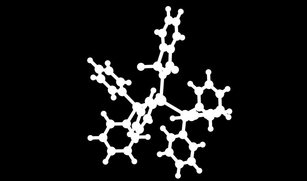
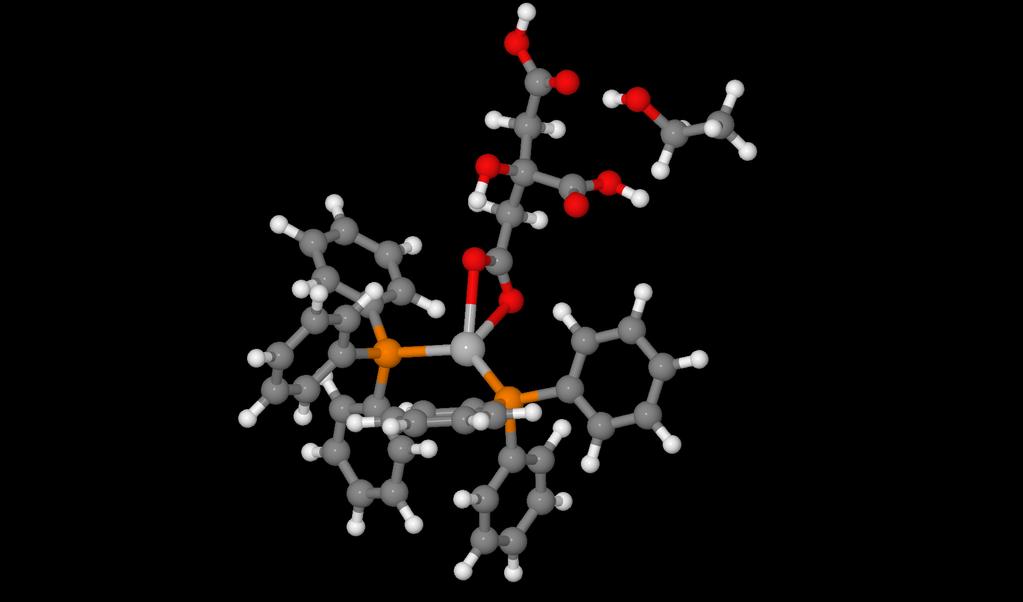
150 136 CHAPTER 7. SILVER-PHOSPHINE MOLECULAR CRYSTAL SYSTEMS (g) Structure 12 (h) Structure 14 (i) Structure 17 (j) Structure 18 (k) Structure 19 (l) Structure 21 (m) Structure 22

151 7.3. CALCULATIONS Calculations Convergence testing Energy cut-off Table 7.2 shows the convergence of calculated couplings in an isolated molecule of structure 2 with respect to the cut-off energy of the plane-wave basis set used (E cut ). As good level of convergence is achieved by E cut = 50 Ry. Inclusion of semi-core orbitals in pseudopotential valence Inclusion of some high lying core orbitals in the valence of a pseudopotential can sometimes improve the accuracy of calculations if they are chemically active. To investigate this, the 4p and 4s orbitals were added to the silver pseudopotential. Table 7.3 illustrates the level of improvement to be had in an isolated molecule of structure 2. The inclusion of both the 4s and 4p in the silver pseudopotential gives a modest increase in the coupling, approximately T 2 J 1. However, this came at the cost of roughly doubling the memory requirements of the calculation due to the extra electrons treated and storage of projector arrays Plane-wave pseudopotential calculations We have calculated J-couplings using both non-relativistic theory and ZORA scalarrelativistic theory with ultrasoft pseudopotentials for all crystals with all atomic positions optimised, a 50 Ry energy cut-off and a single k-point as all cells were

152 138 CHAPTER 7. SILVER-PHOSPHINE MOLECULAR CRYSTAL SYSTEMS Table 7.1: The molecular crystals examined, with references, chemical formulae and, if present, solvent. The molecules are illustrated in Fig Number Reference Formula Solvent No. atoms in cell (Ph 3 P) 2 Ag(NO 3 ) None (Ph 3 P) 2 Ag(NO 3 ) Toluene (1) (Ph 3 P) 2 Ag(NO 3 ) Toluene (2) * (Ph 3 P) 2 Ag(O 2 CCH 2 Ph) None * (Ph 3 P) 2 Ag(O 2 CC(CH 3 ) 3 ) None * (Ph 3 P) 2 Ag(O 2 CCH 2 C(CH 3 ) 3 ) None (Ph 3 P) 2 Ag(O 2 CCH 2 O-C 6 H 3-2,4Cl 2 ) None (Ph 3 P) 2 Ag(NO 2 ) CH 2 Cl (Ph 3 P) 2 Ag(O 2 C(OH)CHCH 3 ) None (Ph 3 P) 2 Ag(NS(O 2 )C 6 H 4 C(O)) None (Ph 3 P) 2 Ag(NS(O 2 )C(CH 3 )C(CH 3 )C(O)) None (Ph 3 P) 2 Ag(CF 3 CO 2 ) None * (Ph 3 P) 2 Ag(C 6 H 7 O 7 ) CH 3 CH 2 OH 196 gb (Ph 3 P) 2 Ag(O 2 COH) None 148 gb {(Ph 3 P) 2 Ag} 2 (CO 3 ) 2H 2 O 296 * Supplied by collaborator Table 7.2: Convergence with respect to the cut-off energy of couplings in an isolated molecule of structure 2. Reduced couplings are given in units of T 2 J 1. E cut / Ry 1 K(Ag P1) 1 K(Ag P2) 2 K(P1 Ag P2) Table 7.3: Illustration of improvement by inclusion of semi-core states in the valence of the ultrasoft pseudopotential in an isolated molecule of structure 2. Reduced isotropic couplings are given in units of T 2 J 1. Ag valence P valence 1 K(Ag P1) 1 K(Ag P2) 4d5s5p 3s3p3d p4d5s5p 3s3p3d s4d5s5p 3s3p3d s4p4d5s5p 3s3p3d

153 7.3. CALCULATIONS 139 of sufficient size to avoid perturbation image effects. Tables 7.4 and 7.5 show the calculated couplings. The non-relativistic predicted values are in poor agreement with experiment, systematically underestimating both 1 K(P Ag) and 2 K(P Ag P). When a relativistic pseudopotential is used on the silver atom both sets of couplings are significantly improved with respect to experiment, although 1 K(P Ag) still systematically underestimates even the lower end of the quoted experimental ranges. There are two effects that can be discussed separately. The first is the indirect effect of relativity on the couplings by its effect on the ground-state electronic structure, which will be visible in changes in the 1 K(P Ag) and 2 K(P Ag P) couplings. This effect has previously been noted studies involving two-bond coupling through a heavy ion. 21 The second is the direct effect of relativity due to the modifications to the coupling perturbation operators, which will be visible in the 1 K(P Ag) couplings. Both of these are present, indirect effects are visible in the increase in the 2 K(P Ag P) couplings, and both direct and indirect effects together, albeit not disentangleable, are in the increase of the 1 K(P Ag) couplings Local orbital calculations In order to determine the source of the remaining source of error with experiment, calculations were performed by including spin-orbit effects and using the PBE0 hyrbid functional. These two extra contributions were shown to be important by Moncho and Autschbach 116 for row six elements. As neither spin-orbit effects nor the use of hybrid functional have been implemented for the calculation of J-coupling tensors in plane-wave pseudopotential codes, a local-orbital code must be used. The

154 140 CHAPTER 7. SILVER-PHOSPHINE MOLECULAR CRYSTAL SYSTEMS Table 7.4: Calculated and experimental isotropic reduced coupling constants (K), in T 2 J 1. For KCalc ZORA silver atoms were treated with relativistic pseudopotentials and ZORA modified operators. Experimental couplings have not been supplied for structures 5 9. Structure Site A Site B K NRel Calc K ZORA Calc K Ag109 Exp K Ag107 Exp 2. Ag P Ag P P 1 P Ag P Ag P P 1 P Ag P Ag P P 1 P Ag P Ag P P 1 P Ag P Ag P P 1 P Ag P Ag P P 1 P Ag and 109 Ag couplings were not resolved separately in experiment.

155 7.3. CALCULATIONS 141 Table 7.5: Calculated and experimental isotropic reduced coupling constants, in T 2 J 1. For KCalc ZORA silver atoms were treated with relativistic pseudopotentials and ZORA modified operators. Structure Site A Site B K NRel Calc K ZORA Calc K Ag109 Exp K Ag107 Exp 12. Ag P Ag P P 1 P Ag P Ag P P 1 P Ag 1 P Ag 1 P Ag 2 P Ag 2 P P 1 P P 3 P Ag 1 P Ag 1 P Ag 2 P Ag 2 P P 1 P P 3 P Ag P Ag P P 1 P Ag P Ag P P 1 P Ag P Ag P P 1 P gb1054 Ag P Ag P P 1 P gb1038 Ag 1 P Ag 1 P Ag 2 P Ag 2 P Ag and 109 Ag couplings were not resolved separately in experiment.

156 142 CHAPTER 7. SILVER-PHOSPHINE MOLECULAR CRYSTAL SYSTEMS Non-relativistic ZORA scalar-relativistic CASTEP K(Ag P) / T 2 J Experiment K(Ag P) / T 2 J 1 Figure 7.1: Experimental versus calculated K(Ag P) J-couplings in various silver molecular crystals. The calculations were performed at a non-relativistic and ZORA scalar-relativistic level of theory. The experimental error bars are derived from the spread in K values for 107 Ag and 109 Ag experiments.

157 7.3. CALCULATIONS CASTEP K(P Ag P) / T 2 J Non-relativistic ZORA scalar-relativistic Experiment K(P Ag P) / T 2 J 1 Figure 7.2: Experimental versus calculated K(P Ag P) J-couplings in various silver molecular crystals. The calculations were performed at a non-relativistic and ZORA scalar-relativistic level of theory. The experimental error bars are derived from the spread in K values for 107 Ag and 109 Ag experiments.

158 144 CHAPTER 7. SILVER-PHOSPHINE MOLECULAR CRYSTAL SYSTEMS Amsterdam density-functional (ADF) code was chosen for its mature relativistic J- coupling implementation allowing both inclusion of spin-orbit effects and use of hybrid functionals. The ADF calculations were performed by Vaida Arcisauskaite, of the Department of Chemistry at the University of Oxford. To reduce computational cost, only isolated molecules were treated. Three molecules with relatively small complexes and possessing a range of couplings, structures 2, 14 and 21, were chosen to be examined. Their structures were created by extracting single molecules from the relaxed crystal structures, thus still taking into account structural effects of crystal packing. The basis set chosen was QZ4P on the coupled atoms and TZ2P on other atoms, there was no frozen core, and a point-like nucleus was used. The functionals used were PW92/PBE and PW92/PBE0 for the groundstate and VWN/PBE and VWN/PBE0 for the first-order response. The calculated couplings are displayed in Table 7.6, alongside scalar-relativistic PBE calculations using Castep for both the full crystal and for the isolated molecule (including any solvent molecule) for comparison and estimation of the effect of the crystal packing on the couplings, and plotted in Fig The inclusion of spin-orbit effects has a small effect on the coupling, a reduction of approximately T 2 J 1 in the 1 K(Ag P) couplings. The use of the PBE0 hyrbid functional, however, has quite a significant effect, increasing the 1 K(Ag P) couplings by approximately T 2 J 1. The scalar-relativistic calculations using the PBE0 functional have the best RMSD agreement with experiment, of and T 2 J 1 for 1 K(Ag P) and 2 K(P Ag P) couplings respectively. The next best are the spin-orbit including relativistic calculations using the PBE0 functional, with RMSDs of and T 2 J 1

159 7.4. CONCLUSIONS 145 respectively. One would expect that going from scalar-relativistic to spin-orbit including levels of theory would improve the agreement with experiment, however it hasn t. This can in fact be explained by the calculations being on isolated molecules rather than the full crystal. We can estimate the effect of being packed in a crystal on the couplings by taking the difference between a plane-wave pseudopotential calculation on the crystal and the same calculation on an isolated molecule, which we shall term the crystal correction (CC). Adding the CC on to the various levels of local-orbital theory, shown in Table 7.7 and Fig. 7.3, shows that the agreement of the spin-orbit level of theory improves to RMSDs of and T 2 J 1 respectively, within the estimated experimental error for the majority of couplings, whereas the agreement of the scalar-relativistic level of theory worsens to RMSDs of and T 2 J 1 respectively. 7.4 Conclusions In this chapter we have demonstrated the ability of the presented plane-wave pseudopotential scalar-relativistic method to predict isotropic NMR J-coupling constants in molecular crystals of moderate size, hundreds of atoms in a unit cell, an advance on methods that, due to computational cost, can only treat small isolated molecules. We have also examined the source of the remaining errors in the calculations, finding that when spin-orbit effects are included, hybrid functionals are used and crystal packing is accounted for, a within-error agreement with experiment is achieved.

160 146 CHAPTER 7. SILVER-PHOSPHINE MOLECULAR CRYSTAL SYSTEMS Table 7.6: Reduced isotropic coupling values, in T 2 J 1, for selected molecules, showing level of improvement in agreement with experiment when including spinorbit effects and using the PBE0 hybrid functional. Experimental errors estimated by spread in reported 107 Ag and 109 Ag couplings. The ADF calculations were performed by Vaida Arcisauskaite, of the Department of Chemistry at the University of Oxford. Structure 2 Castep ADF (molecule) Experiment Site A Site B Crystal Molecule SR PBE SR PBE0 SO PBE SO PBE0 Ag P ± Ag P ± P 1 P ± 7.18 Structure 14 Ag P ± Ag P ± P 1 P ± 0.00 Structure 21 Ag P ± Ag P ± P 1 P ± 0.00 RMSD 1 J(Ag P) RMSD 2 J(P P) Table 7.7: Reduced isotropic coupling values, in T 2 J 1, for the selected molecules with a crystal correction (CC), estimated from the difference between isolated molecule and full crystal Castep calculations, added on to calculations using the PBE0 functional at scalar-relativistic (SR PBE0) and spin-orbit (SO PBE0) levels of theory calculated using the ADF local-orbital code. Root mean-squared deviations (RMSD) from experiment are shown for 1 K(Ag P) and 2 K(P Ag P) couplings. Structure 2 Corrected ADF (molecule) Experiment Site A Site B SR PBE0 + CC SO PBE0 + CC Ag P ± Ag P ± P 1 P ± 7.18 Structure 14 Ag P ± Ag P ± P 1 P ± 0.00 Structure 21 Ag P ± Ag P ± P 1 P ± 0.00 RMSD 1 J(Ag P) RMSD 2 J(P P)

161 7.4. CONCLUSIONS 147 Calculated K(Ag P) / T 2 J Castep crystal Castep molecule ADF SR PBE ADF SR PBE0 ADF SO PBE ADF SO PBE0 ADF SO PBE0 + CC Experiment K(Ag P) / T 2 J 1 Figure 7.3: Comparison of calculated reduced isotropic coupling values, in T 2 J 1, for the selected molecules at various levels of theory against experimental values.

162 148 CHAPTER 7. SILVER-PHOSPHINE MOLECULAR CRYSTAL SYSTEMS

163 Chapter 8 J-coupling in Pb 2 ZnF 6 In this chapter, a theoretical study of J-coupling in lead fluoride systems is presented, based on published experimental papers. Discrepencies between experimentally measured J-couplings and those calculated with the published structures are found and discussed, with relevance to the experimental and theoretical investigation of dynamics. 8.1 Pb 2 ZnF 6 experiments Pb 2 ZnF 6 is a recrystallisation product of the ternary transition metal glass family PbF 2 -ZnF 2 -GaF It has fluorine mobility and anionic conductivity. It was investigated in Ref. 226, where it was noted that the room temperature structure of Pb 2 ZnF 6 had never been fully determined, although it had been previously studied using 1D MAS NMR spectroscopy. 227, 228 In addition, they describe a new transition at above room temperature to a new phase, which they name β-pb 2 ZnF 6. They go on to perform X-ray powder diffraction (XRPD), 19 F NMR, 207 Pb NMR and 67 Zn NMR on Pb 2 ZnF 6 and, with ab-initio calculations, propose a structure for the β 149

164 150 CHAPTER 8. J-COUPLING IN PB 2 ZNF 6 form. The XRPD was performed at T = 25 C and 90 C. The 19 F NMR and 207 Pb NMR was performed at T = 28 C, 57 C, 69 C and 90 C. The 19 F Hahn-echo NMR was performed at T = 70 C and the 67 Zn Hahn-echo NMR was performed at T = 100 C. Their differential thermal analysis (DTA) data suggests that Pb 2 ZnF 6 has two phases: a room temperature phase, α-pb 2 ZnF 6 ; and a higher temperature phase, β-pb 2 ZnF 6. The α phase has a lower symmetry than the β phase, observed as more peaks in the XRPD spectrum of the α phase (T = 25 C) than the β phase (T = 90 C) and a reduction in the number of 19 F and 207 Pb lines in NMR experiments above T = 60 C. Two candidate structures were created by the authors of Ref Structure 1 was derived from the XRPD spectrum and is shown in Fig. 8.1, with the fluorine sites labelled. In this structure of β-pb 2 ZnF 6 there is one lead site, one zinc site, and five fluorine sites. There are alternating layers of corner sharing lead-fluorine tetrahedra and corner sharing zinc-fluorine octahedra. In the zinc-fluorine layers, the Zn and F are arranged in two orthogonal sets of chains, one containing the F2 and the other the F3 fluorine sites. All FX Zn FX have an angle of 180. The F2 chains are described as having a 180 Zn F2 Zn angle and the F3 chains are described as having a Zn F3 Zn angle. Structure 2 is the other structure reported in Ref The density functional forces were minimised using the Wien2k linearised augmented plane-wave (LAPW) code with, as reported, a R MT K max = 8, 100 k-points and with electron exchangecorrelation described by the PBE functional. Forces on ions were minimised to below 1.8 mry per bohr, or approximately 46 mev/å. The lattice vectors were fixed at their experimental values. It was not specified if symmetry constraints were

165 8.1. PB2 ZNF6 EXPERIMENTS 151 F4 F1 F5 F3 F2 Figure 8.1: Unit cell structure of β-pb2 ZnF6 with the fluorine sites labeled, from the XRPD structure (1) determined in in Ref Grey spheres correspond to lead atoms, green to fluorine and blue to zinc.

166 152 CHAPTER 8. J-COUPLING IN PB 2 ZNF 6 Table 8.1: Summary of structural parameters, including standard deviations where appropriate, of the ZnF 6 octahedra in various Pb 2 ZnF 6 models. The parameter ψ is Ghose and Tsang s 216 polyhedral distortion parameter, Eqn Parameter 1. XRPD 2. Wien2k 3. α 4. β F1 Zn F ± ± 0.3 F2 Zn F ± ± 0.3 F3 Zn F ± ± 0.1 F1 Zn F ± ± 0.7 F1 Zn F ± ± 0.5 F2 Zn F ± ± 0.3 Zn F2 Zn ± ± 1.4 Zn F3 Zn ± ± 0.3 F1 Zn / Å ± ± 0.00 F2 Zn / Å ± ± 0.01 F3 Zn / Å ± ± 0.00 ψ ± ± 0.08 applied, but it retains the same symmetry as the unrelaxed XRPD structure. As in structure 1, all FX Zn FX have an angle of 180. The F2 chains are described as having a 180 Zn F2 Zn angle and the F3 chains are described as having a Zn F3 Zn angle. A summary of structural parameters for both structures is given in Table Zn electric field gradients The quadrupolar coupling constant, C Q on the Zn site was experimentally determined in Ref. 226 to be 8.3 ± 0.1 MHz and the quadrupolar asymmetry parameter, η Q was determined to be 0.10 ± Ab-inito caculations using Wien2k are also presented, with C Q = 7.7 MHz and η Q = 0.64 for the XRPD-derived structure (1) and C Q = 9.0 MHz and η Q = 0.06 for the Wien2k-relaxed structure (2). New electric field gradient calculations have been performed with the Castep code129, 146 using a cut-off energy of 50 Ry, the PBE exchange-correlation functional, a single k-

167 8.1. PB 2 ZNF 6 EXPERIMENTS 153 Table 8.2: Zinc quadrupole coupling constants and asymmetry parameters from ab-inito electic field gradient calculations on the proposed structures, using both the Wien2k (reported in Ref. 226) code and Castep code (this work). An updated Wien2k calculation on structure 1 is also presented. 229 Structure Code C Q / MHz η Q 1. XRPD Wien2k XRPD Wien2k new Wien2k Wien2k XRPD Castep Wien2k Castep α Castep 12.7 ± ± 0.17 MD mean 1 Castep MD mean 2 Castep 10.9 ± ± β Castep 11.6 ± ± 0.08 Experiment 8.3 ± ± 0.05 point, and ultrasoft pseudopotentials. The pseudopotential describing the Zn atoms treat the 3s and 3p states in the valence. The C Q and η Q values are presented in Table 8.2, along with the original Wien2k calculations. The agreement of values calculated for structure 1 between codes is poor, Castep predicting C Q = 19.7 MHz compared to 7.7 MHz as reported in Ref The asymmetry parameter η Q are in reasonable agreement, 0.64 versus The agreement between values calculated for structure 2, however, is good and compares well to experiment. Castep predicts C Q = 9.25 MHz, Wien2k predicts C Q = 9.0 MHz and experiment finds C Q = 8.3 ± 0.1 MHz, so both marginally overestimate the quadrupole coupling frequency. The asymmetries are all consistent, being η Q = 0.06, 0.07 and 0.10 ± 0.05 respectively. The cause of the disagreement for structure 1, the XRPD-derived structure, is not clear, however repeats of the calculations 229 using Wien2k give a C Q = 18.6 MHz and η Q = 0.75, both now consistent with the Castep calculations. The Castep predictions are hence consistent with the conclusion in Ref. 226 that the Wien2k-

168 154 CHAPTER 8. J-COUPLING IN PB 2 ZNF K(Pb F5) / T 2 J Fine grid scale = 2 Fine grid scale = Cut-off energy / Ry Figure 8.2: Convergence of a 1 K(Pb F) coupling with respect to the plane-wave basis-set cut-off energy and scale of fine augmentation grid used. A energy cut-off of 40 Ry and fine augmentation grid scale of 4 is determined to give good numerical precision. relaxed structure is most consistent with experiment and most likely provides the best physical description of β-pb 2 ZnF Pb F J-coupling Calculated and experimental 226 J-couplings of all five fluorine sites to the lead site are reported in Table 8.3 for the two β-pb 2 ZnF 6 structures. Calculations were performed using Castep with a converged (see Fig. 8.2) energy cut-off of 40 Ry, one k-point ( 1 4, 1 4, 1 4 ), ZORA ultrasoft pseudopotentials on the heavy ion (Pb) and Schrödinger ultrasoft pseudopotentials on the lighter ions (Zn and F). The inclusion

169 8.1. PB 2 ZNF 6 EXPERIMENTS 155 Table 8.3: J-couplings of all five fluorine sites to their four nearest lead neighbours in the two β-pb 2 ZnF 6 structures given in Ref. 226 (1 and 2). The mean is of the couplings to the underlined sites, which are the largest equivalent couplings. Site J iso / Hz F1 (F63) Pb 17 Pb 19 Pb 20 Pb 21 Mean 1. XRPD Wien2k Experiment 2000 ± 200 F2 (F51) Pb 11 Pb 13 Pb 18 Pb 19 Mean 1. XRPD Wien2k Experiment 1700 ± 200 F3 (F59) Pb 13 Pb 15 Pb 19 Pb 22 Mean 1. XRPD Wien2k Experiment 3000 ± 200 F4 (F75) Pb 18 Pb 19 Pb 27 Pb 29 Mean 1. XRPD Wien2k Experiment 1800 ± 200 F5 (F81) Pb 17 Pb 19 Pb 27 Pb 30 Mean 1. XRPD Wien2k Experiment 1800 ± 200

170 156 CHAPTER 8. J-COUPLING IN PB 2 ZNF 6 of relativity is important for the heavy lead ion, which is in row six of the periodic table. The two structures are in good agreement with experiment for the couplings to lead from the F1, F3, F4 and F5 sites, the XRPD-derived structure (1) generally being better, there being larger errors of the order 800 Hz on sites F1 and F5 for structure 2. However, the 1 J(Pb F2) coupling has serious disagreements for both structures 1 and 2, being roughly 800 Hz versus the 1700 ± 200 Hz observed in experiment. Exact agreement with experiment shouldn t be expected, as both fluorine and lead are known to be difficult to treat, lead likely needing spin-orbit effects to be taken into account and both requiring better descriptions of the electronic exchance-correlation energy. However, one should expect that the Pb F couplings have a consistent systematic error. As the F2 site is the fluorine in the ZnF 6 octahedra with a Zn F2 Zn bond angle of 180, this is a possible indication of interesting dynamics occuring, poorly explained by a simple high temperature structure with average atomic positions. 8.2 Further structural optimisation The two structures (1 and 2) determined in Ref. 226 are clearly insufficient for a good description of the J-coupling between the F2 site and the Pb site. A new relaxation has been performed with lower convergence tolerance using the Castep code with ultrasoft pseudopotentials, a plane-wave basis set described by a cut-off energy of 50 Ry and a k-point spacing of 0.06 Å 1 (giving four k-points) to give structure 3. The forces on the ions were minimised to at most 6 mev/å. The lattice vectors were fixed at their experimental values and there were no symmetry constraints applied. After a number of relaxation steps, spontaneous distortion of the fluorine-zinc layer

171 8.2. FURTHER STRUCTURAL OPTIMISATION 157 (a) View of β-pb2 ZnF6 along the (110) direction. (b) View of α0 -Pb2 ZnF6 along the (110) direction. Figure 8.3: Views of the β and α0 structures along the (110) direction. The F2 chains in the α0 structure have distorted from their original Zn F Zn in the β structure to in the α0 structure.

172 158 CHAPTER 8. J-COUPLING IN PB 2 ZNF 6 F2 chains was observed, see Fig. 8.3 for an illustration. As the DFT relaxation is in effect performed at T = 0 K without symmetry constraints, this likely corresponds to a transition to the low-temperature α-pb 2 ZnF 6 structure. However, as we cannot conclusively assert that this is the α structure, lacking experimental data, and considering possibilities such as DFT error or the true α structure having a different unit cell, structure 3 will hence be named α -Pb 2 ZnF 6. Table 8.1 summarises the structural parameters, bond angles and bond lengths, relating to the ZnF 6 octahedra in the α structure, along with the other models used. The α structure no longer has FX Zn FX exactly equal to 180 nor F1 Zn F2 and F2 Zn F3 precisely equal to 90.0, appearing to prefer a slight distortion of the octahedra. Most significantly, Zn F2 Zn is no longer but rather ± 0.9. We can look at the total energy differences between structures to get an impression of the relative improvement in energetic stability. Based on plane-wave ultrasoft calculations at a 50 Ry cut-off energy and single k-point, the total energy of structure 1 is 2.98 ev above structure 3, and structure 2 is 0.33 ev above structure 3. Divided by the number of ZnF 6 octahedra present in the structure, this is ev and ev repsectively. The per-octahedron difference between structures 2 and 3 is relatively small, within the range of just-above room temperature thermal motion. The β structure, represented by the XRPD and Wien2k-relaxed structures, might hence be a high temperature thermal average, metastable at T = 0 K Zn electric field gradients The quadrupole coupling constant and asymmetry parameter were predicted in the α structure using, as before, a cut-off energy of 50 Ry, the PBE exchange-correlation functional, a single k-point, and ultrasoft pseudopotentials. The pseudopotential

173 8.2. FURTHER STRUCTURAL OPTIMISATION 159 Table 8.4: J-couplings of all five fluorine sites to their four nearest lead neighbours in the α -Pb 2 ZnF 6 structure (3) created in this work. The mean is of the couplings to the underlined sites, which are equivalent in the β structure. Site J iso / Hz F1 (F63) Pb 17 Pb 19 Pb 20 Pb 21 Mean 3. α Experiment 2000 ± 200 F2 (F51) Pb 11 Pb 13 Pb 18 Pb 19 Mean 3. α Experiment 1700 ± 200 F3 (F59) Pb 13 Pb 15 Pb 19 Pb 22 Mean 3. α Experiment 3000 ± 200 F4 (F75) Pb 18 Pb 19 Pb 27 Pb 29 Mean 3. α Experiment 1800 ± 200 F5 (F81) Pb 17 Pb 19 Pb 27 Pb 30 Mean 3. α Experiment 1800 ± 200 describing the Zn atoms treated the 3s and 3p states in the valence. The C Q and η Q values are presented in Table 8.2. As ranges of C Q and η Q were found, a mean and standard deviation are quoted for both. Both C Q = 12.7 ± 1.9 MHz and η Q = 0.36 ± 0.17 systematically overestimate their experimental values, more so than structures 1 and 2. This indicates that, as might be expected, α does not accurately represent the high-temperature β structure Pb F J-coupling Although α likely corresponds to the low temperature structure, we can calculate the J-coupling between the fluorine sites at the lead sites. If the high temperature β structure can be considered to be an average of thermal hopping between α structures, as a simple level of approximation we might take the mean of equivalent

174 160 CHAPTER 8. J-COUPLING IN PB 2 ZNF 6 couplings to produce thermally averaged J-couplings. The J-couplings were calculated, as before, with the Castep code using a 40 Ry plane-wave cut-off energy, one k-point and ZORA ultrasoft pseudopotentials on the heavy ion (Pb) and Schrödinger ultrasoft pseudopotentials on the lighter ions (Zn and F). The calculated J-couplings in α, when averaged over couplings equivalent in the β structure, correspond reasonably for sites F2, F4 and F5, although generally systematically larger. However, the couplings to F1 and F3 have inconsistent errors compared to the high-temperature experiment, F1 overestimating by 1,088 Hz and F3 underestimating by 441 Hz. As noted before, while we might not expect exact agreement with experiment due to the level of theory used, we should expect that the error is roughly systematic across all sites. 8.3 Thermodynamic averaging of NMR parameters It appears that a simple average of equivalent couplings in α is insufficient to describe the J-coupling in β-pb 2 ZnF 6. The hopping approximation will now be relaxed and the full dynamics of Pb 2 ZnF 6 at the appropriate experimental temperature investigated using Born Oppenheimer molecular dynamics (MD). Previous studies have investigated the effect of temperature on NMR parameters in solids using both phonon calculations and molecular dynamics. 141 The limitations of molecular dynamics were noted, especially the short durations of such simulations. However, as the sites of interest in β-pb 2 ZnF 6 are likely to have highly anharmonic behaviour, due to the suspected hopping, phonon based methods will be insufficient. MD was performed with the NVT ensemble, giving constant particle number, volume and temperature, at 70 C, the temperature that the 19 F J-coupling experiments were performed at, using the Castep code. A Nosé-Hoover 230, 231 chain of five ther-

175 8.3. THERMODYNAMIC AVERAGING OF NMR PARAMETERS Pb 17 Pb 19 Pb 20 Pb 21 Pb F / Å ,000 12,000 14,000 16,000 18,000 t / fs (a) Distance from F1 (F63) to neighbouring lead atoms over time Pb 11 Pb 13 Pb 18 Pb 19 Pb F / Å ,000 12,000 14,000 16,000 18,000 t / fs (b) Distance from F2 (F51) to neighbouring lead atoms over time. Figure 8.4: Distance of atoms representing the five fluorine sites to their four nearest lead atoms over the length of the molecular dynamics simulation. The solid lines are running averages of the form g i = f i (1 λ) + g i 1 λ, where λ =

176 162 CHAPTER 8. J-COUPLING IN PB 2 ZNF Pb 13 Pb 15 Pb 19 Pb 22 Pb F / Å ,000 12,000 14,000 16,000 18,000 t / fs (c) Distance from F3 (F59) to neighbouring lead atoms over time Pb 18 Pb 19 Pb 27 Pb 29 Pb F / Å ,000 12,000 14,000 16,000 18,000 t / fs (d) Distance from F4 (F75) to neighbouring lead atoms over time. Figure 8.4

177 8.3. THERMODYNAMIC AVERAGING OF NMR PARAMETERS Pb 17 Pb 19 Pb 27 Pb 30 Pb F / Å ,000 12,000 14,000 16,000 18,000 t / fs (e) Distance from F5 (F81) to neighbouring lead atoms over time. Figure 8.4

178 164 CHAPTER 8. J-COUPLING IN PB 2 ZNF 6 Zn F3 Zn F3 Zn Zn F3 Zn F3 Zn F2 F2 F2 flip F2 F2 F2 Zn F3 Zn F3 Zn Zn F3 Zn F3 Zn F2 F2 F2 F2 F2 F2 Zn F3 Zn F3 Zn Zn F3 Zn F3 Zn Down Up Figure 8.5: Schematic of flipping behaviour observed in the molecular dynamics simulation of Pb 2 ZnF 6. The ZnF 6 octahedra are constrained to minimise their distortion and the F3 sites do not change their vertical position. mostats with a characteristic ionic time of 10 fs was used. The integration time-step was 1 fs for a total time of of 18,960 fs. Electron exchange-correlation was described with the PBE functional and ultrasoft pseudopotentials were used with a plane-wave basis set described by a 50 Ry energy cut-off, with a single k-point. The simulation took 1124 hours of walltime on one node (32 cores) of a Cray XE6 (HECToR) for a total cost of 35,968 CPU core hours. Fig. 8.4 shows the variation of distances between the fluorine sites and nearestneighbour lead atoms over time. It can be observed that around 2 ps and 10 ps in, there are large changes in some atomic distances, often occuring in a way that swaps two neighbouring lead atoms. This corresponds to a flip in the orientation of the ZnF 6 octahedra, moving the F2 atoms from above the plane of Zn to below or vice-versa, illustrated in Fig Estimating the rate of this flip occuring should be approached cautiously due to the short simulation time used, and because the small

179 8.3. THERMODYNAMIC AVERAGING OF NMR PARAMETERS 165 simulation cell used allows the establishment of long-range order with greater ease than the limit of an arbitrarily large cell. However, this indicates that at 70 C, such a flip is likely happening in the real system on a timescale of picoseconds, significantly faster than any relevant NMR timescale (microseconds to milliseconds). Dynamics on such faster timescales means that NMR tensors should be thermally averaged to give the observed parameters. This supports the earlier hypothesis that the β structure is represented by a hopping process between α structures. However, some sites which are considered equivalent in the β structure do not appear to be equivalent in the molecular dynamics samples. The lead atoms shall be referred to by their index in the structure. From the F1 site, Pb 17 and 19 are equivalent, as are Pb 20 and 21, as in the β structure. From the F2 site, Pb 13 and 19 are equivalent, and Pb 11 and 18 are equivalent, whereas in the β structure all the lead neighbours are equivalent. From the F3 site none of the sites appear to be equivalent, and Pb 22 is consistently the closest to the fluorine atom, whereas in the β structure Pb 11 and 13 are equivalent, as are Pb 19 and 22. From the F4 site all the lead atoms are equivalent, swapping in two pairs of Pb 18 and 19 and Pb 27 and 29, as in the β structure. Finally, from the F5 site, Pb 17 and 19 are equivalent, as are Pb 27 and 30, as in the β structure, however sharing a very similar range of bond lengths. What couplings are considered equivalent will affect how we calculate the mean NMR parameters of the sites Estimating errors Configurations from molecular dynamics are serially correlated with some correlation timescale. This means that, in order to get a correct NVT ensemble, the configurations generated by molecular dynamics should be sampled with a temporal separation longer than this correlation timescale, else nearby samples will be too

180 166 CHAPTER 8. J-COUPLING IN PB 2 ZNF 6 similar and not add new information to the mean and the estimated error in the mean will be too small. The error in the mean can be corrected for any remaining serial correlation between samples using reblocking analysis, 232 which will now be outlined. The mean of some property of configuration i, A i, over a run of N timesteps is A = 1 N N A i, (8.1) i=1 and, assuming independence, the variance in the mean is σ 2 ( A ) = σ 2 (A)/N, (8.2) where σ 2 (A) = 1 N N (A i A ) 2. (8.3) i=1 However, the property of configurations might be serially correlated. If the property of configurations has a correlation length of n c, e.g. it is replicated in blocks of n c, then the variance in the mean is actually σ 2 ( A ) = n c σ 2 (A)/N. (8.4) To find the correlation time we block the sequence of configurations into blocks of

181 8.3. THERMODYNAMIC AVERAGING OF NMR PARAMETERS 167 length n and within block j, take the mean A j = 1 A i, (8.5) n where the sum over i runs only over configurations within the block j. i We can then use these blocked means to estimate the variance σ 2 ( A j ) = n N ( A j A ) 2. (8.6) In the limit of large n, we expect the block means to be uncorrelated and σ 2 ( A j ) to be proportional to 1 n. By taking a limit of n to large block size we can attempt to estimate the true error in the mean. The optimal block size, and hence estimated variance, is determined using the method outlined by Wolff 233 and Lee. 234 The pyblock Python package 235 was used to perform the reblocking and choose the optimal block size. Fully decorrelated sampling will be difficult to achieve with the length of time simulated, as there are only two flips present, and hence a likely total correlation time of tens of picoseconds. However, by averaging between equivalent sites it should be possible to get useful mean values, and instead just ensure sampling at an interval longer than the correlation time of the shorter timescale dynamics between flips Zn electric field gradients The ab-inito C Q and η Q in structure 2 were consistent with experiment, structure 3 overestimating by approximately 4 MHz, though with a large standard deviation. By calculating the electric field gradient from sample configurations generated by

182 168 CHAPTER 8. J-COUPLING IN PB 2 ZNF 6 the molecular dynamics run we can also verify that that aspect of the molecular dynamics is consistent with experiment. Properties calculated from the molecular dynamics should be taken with caution, especially as it appears that a good sample of the flipping behaviour has not been achieved, and that the EFG experiments were performed at 100 C rather than 70 C. The electric field gradient at every zinc site present has been sampled every 200 fs for 10 ps from the configurations generated by molecular dynamics, discarding the first 1 ps of configurations to allow for thermodynamic equilibriation with the thermostat, to give a total of 51 samples. The electric field gradient calculations were performed, as before, with a cut-off energy of 50 Ry, the PBE exchange-correlation functional, a single k-point, and ultrasoft pseudopotentials. The pseudopotential describing the Zn atoms treated the 3s and 3p states in the valence. The EFG calculations on the 51 samples each took 30 minutes walltime on one node (24 cores) of a Cray XC30 (ARCHER) for a total cost of 612 CPU core hours. The observed C Q is found by taking the mean of the EFG tensor, Eqn. 3.82, over the samples and then calculating C Q using Eqn. 6.12, and similarly so for the asymmetry η Q. The tensor might also be averaged over all Zn sites present, as they are considered equivalent. However, the principle axis systems of the sites may not be identical, which complicates taking such an average of tensors. With this in mind, Table 8.2 presents two means derived from the molecular dynamics. Mean 1 is the C Q of the mean of the tensors over all samples and all Zn sites, and Mean 2 is the mean C Q of the mean tensors for each Zn site, where the reported error is the standard deviaton of the site C Q means. Both methods for taking means of the C Q give results roughly consistent with experiment, approximately 2 MHz larger than reported but not exhibiting the scale of errors seen in the J-coupling. The asymmetry parameter calculated in Mean 1 is of

183 8.3. THERMODYNAMIC AVERAGING OF NMR PARAMETERS 169 similar magnitude but smaller than the η Q observed experimentally, and in Mean 2 it is larger than experiment but within one standard deviation Pb F J-coupling As with the electric-field gradient, the first 1 ps of MD configurations were discarded to allow for thermodynamic equilibriation of the system with the thermostat. After that, sample structures were taken every 200 fs for a total of 10 ps to give 51 samples. On each of these sample structures, J-couplings were calculated for each of the fluorine sites using, as before, a 40 Ry plane-wave cut-off energy, one k-point and ZORA ultrasoft pseudopotentials on the heavy ion (Pb) and Schrödinger ultrasoft pseudopotentials on the lighter ions (Zn and F). The J-coupling calculations on the 5 51 samples each took 4 hours walltime on one node (24 cores) of a Cray XC30 (ARCHER) for a total cost of 24,480 CPU core hours. Fig. 8.6 plots the sampled isotropic J-coupling between the fluorine sites and neighbouring lead atoms as a function of time. Their mean values are summarised in Table 8.5 along with site averaging. Standard errors for each coupling are given, along with standard errors estimated using a reblocking analysis (Fig. 8.7). The sites have been averaged using the nearest equivalent sites in the β structure to give Mean 1 and with the sites determined to be equivalent from Fig. 8.4 to give Mean 2. The Mean 1 set of averages compares reasonably, though with significant underestimations of the experimental number for sites F2 and F3. Site F1 is overestimated by approximately 400 Hz and site F5 by 800 Hz. The Mean 2 set of averages compares well, with sites F1, 2, 3 and 4 consistently overestimating experiment by between 200 and 400 Hz. The F5 site is still overestimated by approximately 800 Hz.

184 170 CHAPTER 8. J-COUPLING IN PB 2 ZNF 6 The error in the F5 is inconsistent with the apparent systematic error on the other sites, though the coupling between the chosen equivalent pair and the other pair is of very similar magnitude. The mean of all four F5 couplings gives a value of 2012 Hz, consistent with the experimental value of 1800 ± 200 Hz and the systematic error observed on the other sites. Whether or not such an averaging is justified experimentally is unclear, but such complications involving a number of similar magnitude couplings and the assumption of a single experimental coupling could explain the discrepency. Allowing for errors introduced by the incomplete sampling by the molecular dynamics, this might be considered the set with the best agreement with experiment, having a consistent systematic error. If the Mean 2 set is taken to be the most consistent with experiment, reflecting the local structure of β-pb 2 ZnF 6 at 70 C the best, it might be concluded that the true local topology doesn t corresponds to that of the proposed β structures (1 and 2), but rather more that of the mean MD structure, structure 4 or β -Pb 2 ZnF 6, illustrated in Fig This is especially seen in site F3, as the β structures have two of the Pb F couplings as equivalent, but a result more consistent with the systematic errors on the other sites is gained by only considering the largest J-coupling. The mean structure determined by MD should be taken cautiously because, as noted, full sampling of the observed flips is incomplete and might produce a bias. It can be seen that the F2 chains are averaged to a level position between the Zn atoms, similar to β, but with a small displacement in the layer plane. Table 8.1 gives a summary of structural parameters of the β structure. The FX Zn FX are all very close to 180, as in structures 1 and 2 but slightly less so in structure 3. Of all the structures, the PbF 6 octahedra in β appear to have the smallest deviation from regular octahedra, which would be the preferred configuration in isolation, 236

185 8.4. J-COUPLING IN OTHER SIMILAR MATERIALS 171 the F1 Zn F3 angle being 87.7, as opposed to 79.0, 85.7 and 84.7 for structures 1, 2 and 3 respectively and the other angles being closer to This distortion can be quantified more rigorously in terms of Ghose and Tsang s polyhedral distortion parameter, Eqn. 6.15, also given in Table 8.1. The β structure gives the lowest overall distortion of the ZnF 6 octahedra, with a distortion ψ of 0.27 ± 0.08, compared to 0.78, 0.30 and 0.85 ± 0.20 for structures 1, 2 and 3 respectively. Ab-initio EFG calculations on β are given in Table 8.2, the predicted C Q overestimating experiment by approximately 3 MHz, more so than the molecular dynamics average. The predicted asymmetry of η = 0.52 ± 0.08 is also poor compared to the experimental value of 0.10 ± Together these indicate the effect that dynamics has on the EFG, tending to reduce the quadrupole coupling and asymmetry. The β structure does not reflect the symmetry of the β structures. In order to be consistent with the structure and symmetry observed in XRPD in Ref. 226, this must somehow be restored. One possibility would be that the material is spatially disordered between two symmetric orientations, hence giving the correct long-range symmetry. 8.4 J-coupling in other similar materials As a point of comparison for the complex behaviour of couplings in β-pb 2 ZnF 6, two additional materials containing Pb F J-couplings, with experimental measurements, have been examined to estimate the likely systematic errors present. α PbF 2 contains two fluorine sites and one lead site. Two structures were used for α PbF 2, one determined experimentally in Ref. 237 and the other where the ionic positions of the experimental structure have been optimised to minimise ionic forces, keeping the lattice vectors constant, using the PBE functional, a 50 Ry energy

186 172 CHAPTER 8. J-COUPLING IN PB 2 ZNF Pb 17 Pb 19 Pb 20 Pb 21 J(Pb F) / Hz ,000 t / fs (a) J-coupling from F1 (F63) to neighbouring lead atoms over time Pb 11 Pb 13 Pb 18 Pb 19 J(Pb F) / Hz ,000 t / fs (b) J-coupling from F2 (F51) to neighbouring lead atoms over time. Figure 8.6: The solid lines are running averages of the form g i = f i (1 λ) + g i 1 λ, where λ = 0.9.

187 8.4. J-COUPLING IN OTHER SIMILAR MATERIALS Pb 13 Pb 15 Pb 19 Pb 22 J(Pb F) / Hz ,000 t / fs (c) J-coupling from F3 (F59) to neighbouring lead atoms over time Pb 18 Pb 19 Pb 27 Pb 29 J(Pb F) / Hz ,000 t / fs (d) J-coupling from F4 (F75) to neighbouring lead atoms over time. Figure 8.6

188 174 CHAPTER 8. J-COUPLING IN PB 2 ZNF Pb 17 Pb 19 Pb 27 Pb 30 J(Pb F) / Hz ,000 t / fs (e) J-coupling from F5 (F81) to neighbouring lead atoms over time. Figure 8.6

189 8.4. J-COUPLING IN OTHER SIMILAR MATERIALS 175 Standard error / Hz Pb 17 Pb 19 Pb 20 Pb Pb 11 Pb 13 Pb 18 Pb Block size Block size (a) F1 (F63). (b) F2 (F51). Standard error / Hz Pb 13 Pb 15 Pb 19 Pb Pb 18 Pb 19 Pb 27 Pb Block size Block size (c) F3 (F59). (d) F4 (F75). Standard error / Hz Pb 17 Pb 19 Pb 27 Pb Block size (e) F5 (F81). Figure 8.7: Reblocking analysis of molecular dynamics data, discussed in Sec , for each Pb F J-coupling on each of the flourine sites, performed with the pyblock package. 235

190 176 CHAPTER 8. J-COUPLING IN PB 2 ZNF 6 Table 8.5: Mean isotropic J-couplings of all five fluorine sites to their four nearest lead neighbours from samples created from molecular dynamics at 70 C. Mean 1 is of the couplings to the underlined sites, which are equivalent in the β structure, while Mean 2 is of the couplings to the starred sites, which are found to be equivalent in the MD bond length data shown in Fig Site J iso / Hz F1 (F63) Pb 17* Pb 19* Pb 20 Pb 21 Mean 1 Mean 2 MD mean Error Re-blocked error Experiment 2,000 ± 200 F2 (F51) Pb 11 Pb 13* Pb 18 Pb 19* Mean 1 Mean 2 MD mean Error Re-blocked error Experiment 1,700 ± 200 F3 (F59) Pb 13 Pb 15 Pb 19 Pb 22* Mean 1 Mean 2 MD mean Error Re-blocked error Experiment 3,000 ± 200 F4 (F75) Pb 18* Pb 19* Pb 27* Pb 29* Mean 1 Mean 2 MD mean Error Re-blocked error Experiment 1,800 ± 200 F5 (F81) Pb 17 Pb 19 Pb 27* Pb 30* Mean 1 Mean 2 MD mean Error Re-blocked error Experiment 1,800 ± 200

191 8.4. J-COUPLING IN OTHER SIMILAR MATERIALS 177 (a) View of the mean structure determined by molecular dynamics along the (110) direction. (b) View of the mean structure determined by molecular dynamics along the (110) direction. Figure 8.8: Views of the mean structure determined by molecular dynamics, named here as β 0 -Pb2 ZnF6.

192 178 CHAPTER 8. J-COUPLING IN PB 2 ZNF 6 cut-off and a k-point spacing of 0.06 Å 1. The α PbF 2 J-coupling calculations, shown in Tables 8.6a and 8.6b, find a range of four large couplings, from 2650 to 3950 Hz in the case of the experimental structure, from the F1 site to the Pb site. As noted before, the exact outcome of having a range of similar-sized J-couplings on the experimentally measured value is unclear, but the mean value of approximately 3 khz is significantly larger than the 2 khz J-coupling observed in experiment. The F2 site coupling was not measured experimentally. β PbF 2 contains one fluorine sites and one lead site. Only the experimentally determined structure from Ref. 238 was used for α PbF 2, as symmetry enforces zero forces on the ions when the lattice vectors are fixed. The β PbF 2 calculation, shown in Table 8.6c, finds four identical couplings to the closest neighbouring lead atoms, 1 J(Pb F) = 3108 Hz. This is larger than the 2600 Hz value measured experimentally in Ref Overall, couplings in both structures appear to be significantly overestimated by abinito calculation compared to experiment. The magnitude of the systematic error in α PbF 2 and β PbF 2 is consistent with the suggested magnitude of systematic error observed in the Mean 2 set of MD J-coupling Pb 2 ZnF 6 calculations. While the effect of dynamics has been ignored here, these two materials lack the sort of octahedral structures seen in Pb 2 ZnF 6 and so we might expect it to be less important. 8.5 Conclusions Considering the limitations of the techniques used and without further experiments it cannot be definitively asserted which of the proposed models are most consistent with experiment. The nature of the errors in calculated J-coupling, along with

193 8.5. CONCLUSIONS 179 Table 8.6: Calculated and experimental, from Refs. 237 and 239, J-coupling in α PbF 2 and β PbF 2. (a) J-coupling from the F1 site in α PbF 2. F site J iso / Hz F1 (F19) Pb 13 Pb 17 Pb 7 Pb 1 Mean Ref Ions relaxed Experiment 2000 (b) J-coupling from the F2 site in α PbF 2. F site J iso / Hz F2 (F18) Pb 2 Pb 6 Pb 18 Pb 7 Pb 11 Mean Ref Ions relaxed (c) J-coupling from the F site in β PbF 2. F site J iso / Hz F1 (F1) Pb 1 Pb 3 Pb 9 Pb 11 Mean Ref Experiment 2600

194 180 CHAPTER 8. J-COUPLING IN PB 2 ZNF 6 structural effects such as minimisation of the ZnF 6 octahedral distortion by the mean MD structure, suggest that a rich mix of dynamic disorder and spatial disorder could be present in Pb 2 ZnF 6. Despite the lack of a definitive conclusion, this study demonstrates the power of ab-initio J-coupling combined with molecular dynamics to probe and distinguish detailed models of materials. The theoretical techniques developed in this thesis, J- coupling with ultrasoft pseudopotentials and incorporating relativistic effects, brings such a study into the range of reasonable cost with modern computing resources. It should provide a blueprint for future combined theoretical and experimental work investigating the structure of similar materials.

195 Chapter 9 Conclusions and future work In this thesis, the plane-wave pseudopotential method for the prediction of NMR J- coupling in condensed matter was developed to allow the use of state-of-the-art ultrasoft pseudopotentials. Furthermore, additional theory was incorporated to include the effects of special relativity on J-coupling, critical, as shown, for heavy elements. The method can now predict experimentally measured J-coupling with favourable accuracy compared to equivalent all-electron, local orbital basis-set quantum chemistry methods. By being able to treat more diverse systems for a lower cost and with greater ease, the method should now see greater use in the wider NMR crystallography community. In addition, several novel studies into compositional disorder, molecular crystals and dynamic disorder have demonstrated the method s power in combination with experiment for the creation and validation of structural models of materials. The direction of future work is indicated by consideration of the remaining sources of error. The use of approximate exchange-correlation functionals appears to be the main source of error in the systems examined, in agreement with previous studies

196 182 CHAPTER 9. CONCLUSIONS AND FUTURE WORK This will be difficult to fix, due to the high computational cost of higher levels of theory, such as hybrid functionals, especially in plane-wave basis sets. Cheaper corrections, such as the DFT+U method, 84 might be considered as a compromise. The lack of spin-orbit coupling appears to be the next largest source of error in the systems considered. Recent developments in plane-wave pseudopotential codes to allow for the use of two-component spinor wave functions should enable the implementation of PAW J-coupling with spin-orbit effects included An extension to the PAW method to allow for the use of four-component Dirac operators could then be developed, circumventing the need to use the ZORA approximation. Finally, all the calculations performed in this thesis had to be performed using a supercell, due to the problem of perturbations interacting with their own periodic images. This negates some of the computational advantages of a plane-wave pseudopotential approach using Bloch s theorem, leading to cubic scaling in system size rather than linear scaling in k-points. Development of a method to properly treat the incommensurate magnetic perturbation will allow the efficient treatment of crystals with small primitive unit cells and permit convergence to infinite supercell sizes.

197 Appendix A Ab-initio magnetic resonance file format A.1 Introduction The aim of this appendix is to describe the motivations for and definition of a standardised output format for magnetic resonance calculations developed during this thesis. It was felt that as more computational codes incorporate the prediction of NMR parameters, especially for solid-state systems, a unified output format would create a common platform for the further development of tools, such as interfaces to spin simulation codes, visualisation tools and general post processing programs useful in the course of research. It was decided that the format should be machine readable, as simple as possible and provide a complete archival format. The simplicity and machine readability are intended to allow any researcher with a moderate knowledge of a programming language to write their own parser of the format, and so not be reliant on others 183

198 184 APPENDIX A. AB-INITIO MAGNETIC RESONANCE FILE FORMAT doing so, and the completeness of the format is intended to contribute to achieving wider goals relating to scientific reproducibility, e.g. as supplementary information for a journal article, and data mining of simulation output. These goals were developed into some concrete requirements: allowing the easy extraction of information using standard command-line utilities available in distributions of Linux, such as grep and awk; ignoring unrecognised elements, allowing later extension; not to specify redundant information, to reduce maintenance; that properties are specified in full Cartesian tensors in well-defined units, leaving tasks such as finding eigenvalues to further processing; including information on atomic positions and, optionally, the crystal lattice for completeness and to allow visualisation; specifying but not requiring the understanding of symmetry operations; to avoid overly expressive languages such as XML, to guarantee easy parsing. In addition, the following limitations to the standard were recognised: only parameters related to NMR of diamagnetic materials have been specified, the extension to include parameters related to paramagnetic materials should be straight forward; it doesn t include definitions for providing EPR parameters, but could be incorporated in a future backwards-compatible update to the standard; and while the format is designed for processing and archiving, it s not designed for easy querying in a database form. It s assumed a database will perform further transformations into its own desired internal format for indexing. A.2 Specification The file format settled on is essentially a series of blocks consisting of rows constraining whitespace-delimited records, with datatype distinguished by tags in the first column. To allow easier recognition by parsers, the file must start with

199 A.2. SPECIFICATION 185 #$magres-abinitio-v1.0 the version number 1.0 referring to this standard. Minor version number increases after the period will aim to not break backwards compatibility with existing parsers whereas major version number increases before the period may. A.2.1 Blocks Blocks are wrapped with tags: [block]... data... [/block] They cannot be nested or overlap. Unrecognised blocks should be ignored, so as to allow other data to be put in the same file. Blocks discussed in this specification are [atoms] - Atomic coordinates and optional lattice. Must be first block for easy parsing [magres] - Calculated magnetic resonance parameters [calculation] - Calculation metadata such as code version and input parameters The [atoms] block should appear before [magres] for ease of parsing. The feature of ignoring unrecognised blocks allows codes to include extra blocks of text, such as old magnetic resonance file types that have to be retained for backwards compatibility with existing parsers. Input files could also be kept in extra unrecognised blocks.

200 186 APPENDIX A. AB-INITIO MAGNETIC RESONANCE FILE FORMAT A.2.2 Characters and numerical representation This file format is based on 8-bit ASCII characters but only characters should be used outside of comments. Numbers should be written in decimal or scientific notation with double precision (i.e. typically 16 significant figures). Numbers should be written as to be easily parsable by standard string routines (e.g. Fortran, C, Python, Perl, etc.) A.2.3 Records A record is a line in the file of arbitrary length and terminated by the line feed character (\n). Whitespace (characters recognised by \s in a regex) is ignored at the start and end of a line. One or more whitespace characters separate two entries in a record. Each record has a tag, which is the first entry. lattice In the above record, lattice is the tag. A.2.4 Comments Any characters following a # symbol in a line should be ignored. A.2.5 Units Although this specification document will specify the units for each parameter, it s preferable to explicitly define the units used for each kind of tag for discoverability and so as to allow some flexibility and allow parsers to hard-fail when unrecognised units are used. The tag for units is:

201 A.2. SPECIFICATION 187 units <tag> <units> where the units is some case-sensitive string that would make sense to a parser and human, e.g au for when atomic units have been used. The strings should be strictly compared, i.e. J.mol-1 is not the same as Jmol^-1. The units tag must appear once or not at all before the first instance of the tag it is describing. Parsers should warn if they do not recognise units. If they have to process quantities with units they don t recognise they should fail. A.2.6 atoms block The crystal lattice can be given as the a, b, c unit cell vectors. This is an optional element, however if it is not present it can be assumed that the structure is nonperiodic. We will standardise on ångström as the output unit. units lattice Angstrom lattice a1 a2 a3 b1 b2 b3 c1 c2 c3 The atomic positions (for all the atoms in the full crystallographic unit cell) are given in Cartesian coordinates, standardised to ångström as the output unit. These must be present in a file before any magres parameters. units atom Angstrom atom <atom type> <atom label> <number in atom type> x y z The atom type should be an element symbol (no isotopes, i.e. H rather than D) and the atom label can be any string, e.g. the crystallographic label. If there is no label the element symbol should be given again. Atom types can be specified in any order, but the numbers in the type should be in order and start from one.

202 188 APPENDIX A. AB-INITIO MAGNETIC RESONANCE FILE FORMAT If symmetry operators are known, you can specify them with the symmetry tag: symmetry <symmetry string> where the symmetry string is in x,y,z notation. As it is undesirable to require basic scripts to know and be able to apply symmetry operators, all non-unique atoms should still be included. An example set of symmetry operations for an alanine crystal structure would be symmetry x,y,z symmetry x+1/2,-y+1/2,-z symmetry -x,y+1/2,-z+1/2 symmetry -x+1/2,-y,z+1/2 A.2.7 magres block ms - Magnetic shielding The magnetic shielding tensor is defined as the ratio between this induced field, and the external applied field. B in (R) = σ(r) B ext (R), (A.1) σ(r) is a dimensionless quantity which is reported in parts per million (ppm). It is a rank-2 tensor defined for each atomic site and specified by 9 independent Cartesian components. Note that it is not a symmetric tensor but can be written as the sum of symmetric and antisymmetric tensors. units ms ppm ms <atom type> <number in atom type>

203 A.2. SPECIFICATION 189 Where the XY indices label the components of the tensor like (A.2) efg - Electric field gradient The Electric Field Gradient (EFG) is a rank-2, symmetric, traceless tensor V (R) given by V (R) = E α(r) r β 1 3 δ αβ γ E γ (R) r γ, (A.3) where α, β, γ index the Cartesian coordinates x,y,z and E(R) is the local electric field at the position R. The EFG is recorded in atomic units. Note that 1 a.u. of EFG is approximately V m 2. units efg au efg <atom type> <number in atom type> A code might provide the EFG decomposed into theory-dependent contributions with additional tags, e.g. efg ions for just the contribution from the atomic nuclei and cores. isc - Indirect spin-spin coupling (J-coupling) The indirect spin-spin coupling tensor is obtained from the magnetic field induced at nucleus A due to the perturbative effect of the magnetic moment, µ B, of nucleus

204 190 APPENDIX A. AB-INITIO MAGNETIC RESONANCE FILE FORMAT B, B in (R A ) = K A,B µ B (A.4) K A,B is known as the reduced spin coupling tensor. It is a rank-2 tensor, and is given in units of T 2 J 1. The J-coupling tensor is obtained from this using J A,B = 2π hγ A γ B K A,B where γ A is the gyromagnetic ratio of the nucleus A. Note that K (and hence J) is not symmetric but can be written as the sum of symmetric and antisymmetric tensors. The tensors K A,B and K B,A are different. The symmetric part is unchanged on exchanging sites A and B, but the antisymmetric part will change sign. units isc 10^19.T^2.J^-1 isc <atom type A> <number in atom type A> <atom type B> \ <number in atom type B> A code might provide the K-tensor decomposed into theory-dependent contributions with additional tags. sus - Macroscopic magnetic susceptibility The Macroscopic Magnetic Susceptibility of the sample. This is a single rank-2 tensor reported in units of 10 6 cm 3 mol 1 units sus 10^-6.cm^3.mol^-1 sus

205 A.2. SPECIFICATION 191 A.2.8 calculation block The exact content of this section is not precisely defined as applications are not clearly defined, however we suggest it contain sufficient information for a user to reproduce the calculation. For a calculation using a plane-wave pseudopotential code this might include: the date the calculation was performed; the version of computational code used; pseudopotential descriptions; plane wave cut-off energy; k-point sampling. An example from a recent calculation is given in Section A.2.9. Other possible calculation data to include, for example, would be a list of hashes of the input files for cross referencing in a database. A.2.9 Example Below is an example output file from a J-coupling calculation in an ethanol molecule using the Castep code, with the C2 atom acting as the perturbation. It has been marginally edited down in order to fit the width of the page better, and so the numbers given do not necessarily reflect the true level of numerical precision. Line continuations are indicated by a backslash. #$magres-abinitio-v1.0 [calculation] calc_code CASTEP calc_code_version 8.0 calc_code_hgversion 0b4b78c \ Sun, 17 Aug :49: calc_code_platform linux_x86_64_gfortran4.8-xt calc_name ethanol

206 192 APPENDIX A. AB-INITIO MAGNETIC RESONANCE FILE FORMAT calc_comment calc_xcfunctional PBE calc_cutoffenergy ev calc_pspot H UU(qc=6.4,schro)[] calc_pspot C UU:21UU(qc=6,schro)[] calc_pspot O UU:21UU(qc=7.5,schro)[] calc_kpoint_mp_grid 111 calc_kpoint_mp_offset [/calculation] [atoms] units lattice Angstrom lattice units atom Angstrom symmetry x,y,z atom H H E E E-01 atom H H E E E-01 atom H H E E E-01 atom H H E E E+00 atom H H E E E-01 atom H H E E E+00 atom C C E E E-03 atom C C E E E-01 atom O O E E E+00 [/atoms] [magres] units isc 10^19.T^2.J^-1 isc C 2 H E E E E E+00 \

207 A.2. SPECIFICATION E E E E-01 isc C 2 H E E E E E-01 \ E E E E-01 isc C 2 H E E E E E-01 \ E E E E-01 isc C 2 H E E E E E+01 \ 6.054E E E E+01 isc C 2 H E E E E E+01 \ 4.693E E E E+01 isc C 2 H E E E E E+00 \ E E E E-01 isc C 2 C E E E E E+01 \ 1.812E E E E+01 isc C 2 C E E E E E+03 \ 6.914E E E E+03 isc C 2 O E E E E E+01 \ 5.442E E E E+01 [/magres]

208 194 APPENDIX A. AB-INITIO MAGNETIC RESONANCE FILE FORMAT

209 Appendix B Magres processing library B.1 Introduction This appendix describes a library 245 written, and used, in the Python programming language for the processing of the output of magnetic resonance calculations. It was developed during the course of this thesis work and was used in numerous places to automate the creation of results from the raw data. The output of an ab-initio magnetic resonance simulation is relatively modest in terms of pure quantities of data, but can be overwhelming for processing by hand, giving a 3 3 tensor for each of N atoms from a magnetic shielding calculation, the same again for an EFG calculation and N 1 tensors for every J-coupling perturbation site. The recent development of the ab-initio magnetic resonance file format (Appendix A) makes it easy for someone familiar with a programming language to parse the file and load the data into some sort of datastructure for further processing. However, given that there are many common operations then performed, such as measuring bond angles, selecting subsets of atoms, or calculating eigen- 195

210 196 APPENDIX B. MAGRES PROCESSING LIBRARY values, it seems sensible to provide an optional support library that supplies this functionality. The library will be outlined below, along with some practical examples used in the course of this thesis. B.2 Outline The Python language allows program code to be grouped together into modules, which are isolated namespaces that can be loaded into other Python programs. The modules and their contents are: magres.format Class, MagresFile, and associated helper functions for parsing the ab-initio magnetic resonance file format. For example, reading a file in: f = MagresFile ( open (" test. magres ")) magres.atoms Classes, MagresAtoms and MagresAtomsView, that hold collections of atoms, with an optional crystal lattice, and with operations such as selecting atoms of different species or within a certain distance of a point. For example, loading a magres file in and building the datastructure: atoms = MagresAtoms. load_magres (" test. magres ")

211 B.2. OUTLINE 197 Selecting the Al15 atom by species and index using the property shortcut: atom = atoms. Al15 or selecting all Si atoms present within 3.5Å of the Al15 atom, demonstrating selector chaining: Si_atoms = atoms. species ("Si"). within ( atoms.al15, 3.5) magres.atom Class, MagresAtom, that describes an atom, including data such as position and species, and acts as a container for other property objects. atom = atoms. Ag1 print atom print " position =", atom. position print " isotope =", atom. isotope print " gamma109 =", atom. gamma atom. isotope = 107 print " gamma107 =", atom. gamma with the output 109Ag1 position = [ ] isotope = 109 gamma109 = gamma107 = As can be seen, there is support for easily modifying the isotopes of nuclei, which then has knock-on effects in the calculation of nuclear constants such as the gyromagnetic ratio, γ.

212 198 APPENDIX B. MAGRES PROCESSING LIBRARY magres.ms Class, MagresAtomMs, that holds the magnetic shielding tensor and allows easy computation of derived information, such as eigenvalues, the isotropic shift and the chemical shift anisotropy. For example, the following code prints the isotropic magnetic shielding and anisotropy for every proton in the system: for atom in atoms. species ("H"): print atom.ms.iso, atom.ms. aniso magres.isc Class, MagresAtomIsc, that holds the reduced J-coupling tensors between two atoms and allows easy computation of derived quantities such as the full J-coupling tensor and the isotropic coupling. The following code prints out the isotropic part of the J tensor between two atoms: print atoms.c2.isc [ atoms.o1 ]. J_iso magres.efg Class, MagresAtomEfg, that holds the electric field gradient tensor and allows easy computation of derived information, such as eigenvalues, the quadrupole coupling frequency and the asymmetry. The following code, for example, produces a list of the C Q of every Al atom in the system: atoms. species ("Al"). efg.cq This could then be fed into a plotting system or statistics function.

213 B.3. EXAMPLES 199 magres.constants A collection of magnetic resonance data, such as nuclear gyromagnetic ratios and quadrupole moments, and useful functions for operations such as converting a K tensor to a J tensor. For example, the gyromagnetic ratio of 35 Cl is obtained by: print magres. constants. gamma ["Cl", 35] giving the value of magres.utils A collection of utility functions useful in the course of writing scripts using the library, such as a function to find all magnetic resonance output files below a point in a directory hierarchy. B.3 Examples B.3.1 Electric field gradients in disordered system The analysis on gehlenite in Chapter 6 involved ab-initio calculations of electric field gradients in 25 structures per set, followed by extraction of the tensors and structural statistics from every aluminium site present in the material. It s clearly desirable to automate this. Code to perform this will be described below, broken up with explanatory text. First, the relevant pieces of modules are loaded. from magres. utils import load_ all_ magres from matplotlib. pyplot import hist

214 200 APPENDIX B. MAGRES PROCESSING LIBRARY Then, the.magres output files are loaded in from the filesystem as a list of MagresAtoms objects using the load all magres utility function. orig_structures = load_all_magres ( files / orig ) We can do a simple plot of the C Q data on all the Al sites present, using the hist function from the matplotlib module. all_cqs = [] for atoms in orig_ structures : all_cqs += atoms. species ( Al ). efg.cq hist ( all_cqs, bins =20) Next, we write a function to bin the C Q of each aluminium atom by the type of site, T1 or T2, and how many neighbouring silicon atoms there are within 3.5Å. def bin_sites ( structures, bins ): for i, atoms in enumerate ( structures ): for Al_atom in atoms. species ( Al ): neighbours = atoms. species ([ Al, Si ]). within ( Al_atom, 3.5) if len ( neighbours ) == 5: site = T1 else :